Abstract
An accurate understanding of urban objects is critical for urban modeling, intelligent infrastructure planning and city management. The semantic segmentation of light detection and ranging (LiDAR) point clouds is a fundamental approach for urban scene analysis. Over the last years, several methods have been developed to segment urban furniture with point clouds. However, the traditional processing of large amounts of spatial data has become increasingly costly, both time-wise and financially. Recently, deep learning (DL) techniques have been increasingly used for 3D segmentation tasks. Yet, most of these deep neural networks (DNNs) were conducted on benchmarks. It is, therefore, arguable whether DL approaches can achieve the state-of-the-art performance of 3D point clouds segmentation in real-life scenarios. In this research, we apply an adapted DNN (ARandLA-Net) to directly process large-scale point clouds. In particular, we develop a new paradigm for training and validation, which presents a typical urban scene in central Europe (Munzingen, Freiburg, Baden-Württemberg, Germany). Our dataset consists of nearly 390 million dense points acquired by Mobile Laser Scanning (MLS), which has a rather larger quantity of sample points in comparison to existing datasets and includes meaningful object categories that are particular to applications for smart cities and urban planning. We further assess the DNN on our dataset and investigate a number of key challenges from varying aspects, such as data preparation strategies, the advantage of color information and the unbalanced class distribution in the real world. The final segmentation model achieved a mean Intersection-over-Union (mIoU) score of 54.4% and an overall accuracy score of 83.9%. Our experiments indicated that different data preparation strategies influenced the model performance. Additional RGB information yielded an approximately 4% higher mIoU score. Our results also demonstrate that the use of weighted cross-entropy with inverse square root frequency loss led to better segmentation performance than when other losses were considered.
1. Introduction
To build resilient and sustainable cities, geometrically accurate three-dimensional (3D) models are essential for urban planning. We need to segment objects, such as buildings, vegetation, roads and other relevant classes, in large 3D scenes for monitoring infrastructure to, for example, control the growth state of the vegetation growing around critical infrastructures, such as overhead power lines and railroad tracks. Light detection and ranging (LiDAR) is a technology with a promising potential to assist in surveying, mapping, monitoring and assessing urban scenes [1]. In recent years, the MLS has been developed to enable the capture of 3D point clouds of large-scale urban scenarios with higher spatial resolution and more precise data.
Our dataset was acquired with the MLS system, which operates efficiently from a moving platform throughout the roadway and surrounding area in the city of Freiburg. MLS point clouds are usually characterized by complex scenes, large data volume and uneven spatial distribution. Moreover, compared with 2D images that are characterized by their regular data structure, a point cloud is a set of unordered 3-dimensional points [2]. Therefore, several significant challenges exist in urban modeling to process large-scale MLS point clouds automatically [1,3,4,5,6], such as outliers, noise and missing points; uneven point density; occlusions and limited overlap; and large data volume.
All of these challenges come with significant effects regarding the robustness of MLS point cloud processing in urban 3D modeling. To overcome these problems, a great deal of effort has been put into developing methods for automating point cloud interpretation. The two main tasks are: extract semantic information about the 3D objects, while also converting raw scan data into computer-aided design (CAD) geometry [3]. In this paper, we focus on the first issue.
Although early work on the semantic segmentation of point clouds has been mostly conducted with handcrafted features, which can be combined with machine learning methods, such as support vector machine (SVM) or random forest (RF); these approaches often require a large amount of human intervention due to the specific tasks and complexities of MLS point clouds. Recently, computer vision and machine learning have been two of the most popular and well-studied scientific fields. Many studies have gone into facilitating deep-learning methods that can be applied to semantic segmentation on raw MLS point clouds. Although these techniques have achieved impressive performance, they still have two notable drawbacks as to whether they can precisely segment diverse objects from actual urban scenes: Firstly, they have been mainly tested on public benchmarks, which means that the same scenes are used for both training and testing. Cross-scene (objects across different datasets or scenes) segmentation is a conspicuous challenge in processing urban MLS point clouds. For example, high-rise buildings are frequently found in city centers, whereas low-rise buildings are usually observed in the countryside. The road furniture, such as poles and fences, might show in various sizes due to their different appearance forms. Secondly, actual application scenes indicate extremely distorted distributions due to the natural class imbalance observed in real-life scenes. For example, MLS point clouds acquired from a street scene in cities are usually dominated by a large amount of ground or buildings. In addition, objects, like poles, barriers and other road furniture, mostly provide few points as their sizes are relatively small and natural instances relatively low. Therefore, these classes, which are sparse yet significant, have a deficiency.
Taking into account these challenges, we aim to assess the potential of state-of-the-art deep learning architectures on large-scale point clouds from MLS platforms to map urban objects within real-life scenarios. We develop a new large-scene point clouds dataset with point-wise semantic labeled annotation that presents an actual urban environment in Germany, consisting of about 390 million points and 11 semantic categories. In particular, we consider meaningful object categories that are significant to the applications for smart cities and urban planning, such as traffic roads and pavements and natural ground or low vegetation versus high vegetation. Furthermore, we adapt a semantic segmentation method (ARandLa-Net) to simultaneously segment and classify these classes.
Our main research question is as follows: How well does the adapted state-of-the-art DL approach RandLA-net [7] perform on our outdoor large-scale urban datasets in the real world? Moreover, how useful is the DL method in practical problems, such as the challenge of datasets with an imbalanced class distribution? Therefore, we annotated the entire dataset. Then, we assessed several features (i.e., from only 3D coordinates and from both 3D coordinates and RGB values), the impact of different strategies of data preparation and performance gaps between varying loss.
2. Related Work
With the development of DL-based segmentation approaches of 3D point clouds, a larger-quantity and higher-quality annotated dataset is required. Although there are already 3D benchmarks available for the semantic segmentation and classification of urban point clouds, they are very heterogeneous. For example, the Oakland 3-D Point Cloud dataset [8] has only 1.61 million points, which is much less dense than our dataset, and only five classes were evaluated in the literature (there are 24 in the 44 categories that contain sample points below 1000). In the Paris–Lille–3D dataset [9], only points within approximately 20 m away from the road centerline are available. This is different from our dataset, which keeps all acquired points in real-world scenarios within about 120 m without any trimming. The Toronto–3D dataset [10] mainly focuses on the semantic segmentation of urban roadways, and its coverage is relatively small compared to ours.
The aim of semantic segmentation is to divide a point cloud into several subsets and to attribute a specific label to each of them. It requires the understanding of “both the global geometric structure and the fine-grained details of each point” (such as ground, road furniture, building, vehicle, pedestrian, vegetation, etc.) [11]. Therefore, this method is more suited for real-life applications, such as monitoring, city modeling or autonomous driving [12].
According to [11], the broad category of point cloud segmentation can be further subdivided into part segmentation, instance segmentation and semantic segmentation. For the sake of simplicity, this work focuses only on the last of these methods. Within semantic segmentation as a method, there are three main paradigms: voxel-based, projection-based and point-based methods.
Voxel-based approaches: One of the early solutions in DL-based semantic segmentation is combining voxels with 3D convolutional neural networks (CNNs) [13,14,15,16,17,18]. Voxelization solves both unordered and unstructured problems of the raw data. Voxelized data as dense grids naturally preserve the neighborhood structure of 3D point clouds and can be further processed by the direct application of standard 3D convolutions, as in the case of pixels in 2D neural networks [19]. However, comparing with point clouds, the voxel structure is in a low-resolution form. The voxelization steps natively result in a loss of detail within data representation. Nevertheless, a high resolution usually leads to high computation and memory usage. Therefore, it is not easy to scale large-scale point clouds in practice.
Projection-based methods all make the common assumption that the original 3D point data has been adapted to form a regularized structure, either by discretising a point cloud (e.g., in voxel grids) or by using an arrangement of 2D images (RGB-D or multi-view) to represent the 3D data [20,21,22,23]. However, as the underlying geometric and structural information are very likely to be lost in the projection step, this kind of technique is not suitable for learning the features of relatively small object classes in large-scale urban scenes.
Point-based architectures. PointNet [24] and PointNet++ [25] are seminal papers in the application of DNNs for unstructured point clouds. In recent years, a vast amount of other point-based methods [7,26,27,28,29,30,31,32] have been developed. Generally, they can be divided into pointwise MLP methods, point convolution methods, Recurrent Neural Network (RNN)-based methods and graph-based methods. This class of networks has shown promising results in semantic segmentation on small point clouds. In comparison to both voxel-based and projection-based approaches, these workflows appear to be computationally efficient and have the potential to learn per-point local features.
3. Materials and Methods
3.1. Study Area and Data Acquisition
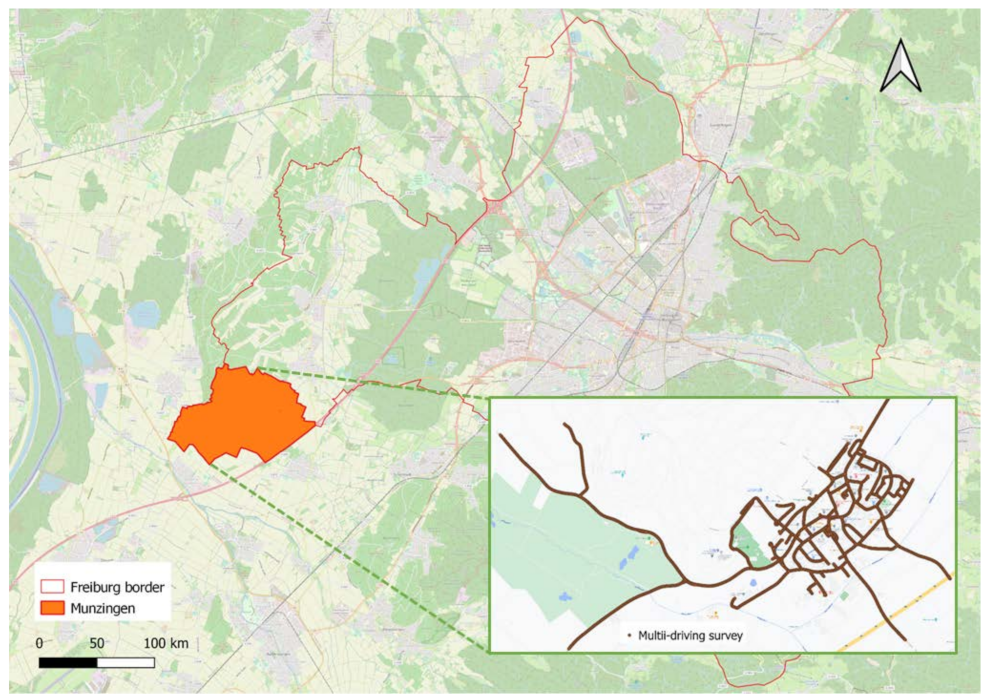
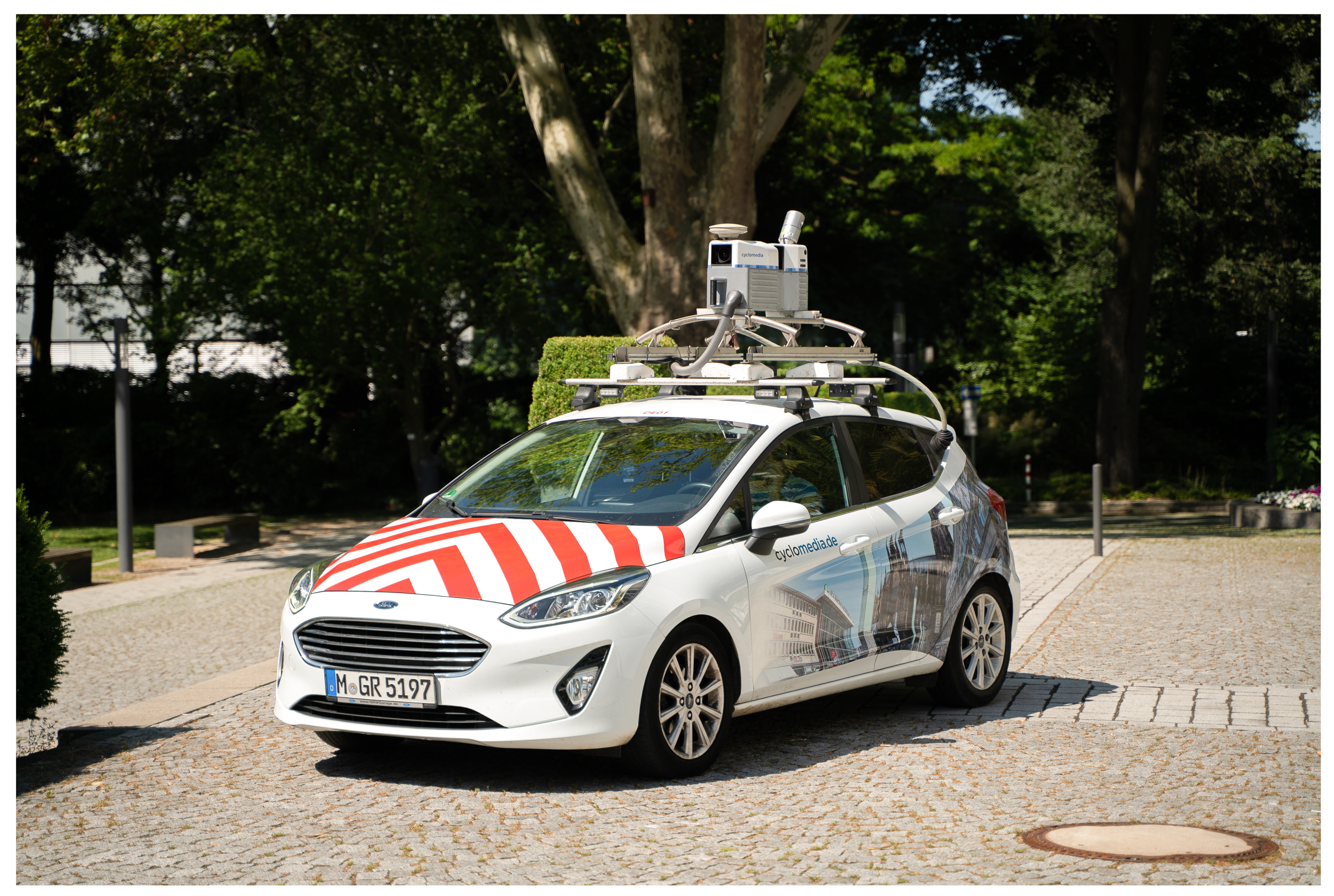
The dataset is a part of the data acquired through the MLS technique by the Vermessungsamt (Land Surveying Office) of the city of Freiburg. The study area of Munzingen belongs to Freiburg, which is one of the four administrative regions of Baden-Württemberg, Germany, located in the southwest of the country; see Figure 1. The Velodyne HDL-32E, with 32 laser beams, acquired point clouds mounted at an angle of 25° on the front roof of the car shown in Figure 2.
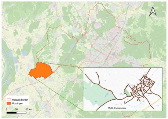
Figure 1.
Point clouds acquired from Munzingen, a suburban region of the city of Freiburg, Germany. This represents a typical suburban European city, covering an area of more than two square kilometers. Brown lines indicate the trajectories of the experimental vehicle during acquisition in Munzingen. OpenStreetMap is loaded as a base map.
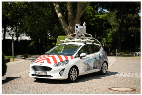
Figure 2.
The Freiburg Munzingen dataset was generated through systematic and comprehensive travel in Freiburg with the Velodyne HDL-32E equipped vehicles.
The LiDAR system can emit a maximum of 700,000 laser pulses per second (note: not every pulse is reflected) with a 120 m (in all directions) maximum shooting distance and a 60 m (above the device height) average vertical shooting distance. With each reflected pulse, the system registers how long it takes for it to be scattered back. Using this information, each impulse is converted into one or more points with x, y, and z coordinates. Then, the point cloud is constructed from these points in three dimensions. The location accuracy of all recording locations shows a mean standard deviation of 10 cm in all directions.
In areas with a high point density, points that are recorded from a greater distance are filtered out. The number of points per square meter depends on the speed of the vehicle being driven, the location, the position of the surface and the number of reflections per pulse. Table 1 indicates the number of points and is based on a single feedback per pulse. In addition, the LiDAR data acquisition takes place at the same time as the regular cyclorama recording, in which a 360° panorama image is generated every 5 m. Based on these cycloramas, each point of the LiDAR point cloud is given a color value.

Table 1.
Point density. The points/m2 are averaged. Ground: directly behind the receiving vehicle. Wall: a vertical surface that is 10 m away from the recording device and facing towards the recording device. Ceiling: a horizontal surface 4.5 m away directly above the recording path.
The dataset covers approximately 2.2 km2 of the neighborhood of Munzingen and shows a rather homogeneous scene that includes residential (mainly) and commercial buildings, vegetation of different types, traffic roads, sidewalks, street furniture and vehicles. The dataset consists of approximately 390 million points in total, which were distributed over and saved separately in 766 individual .las files. Apart from the respective x-y-z coordinates, the dataset also includes a number of features per point, such as the GPS time, three 16-bit color channels, the intensity of the laser beam, point source ID, NIR (near infrared) channel, number of returns and the edge of the flight line. However, apart from the spatial coordinates and RGB information, none of these features will be necessary during training and testing.
3.2. Reference Data Annotating
Training and evaluation of the adapted RandLA-Net (ARandLA-Net) segmentation algorithm require labeled 3D point cloud data. We manually label each point an individual class to ensure the point-wise accuracy of reference data. For example, it does not contain any biases from different segmentation approaches as that could be exploited by the classifier and weaken its effects with other training data, as well as avoids inherited errors; however, this strategy is time-consuming. In addition, it is harder for human beings to mark a 3D point cloud manually than 2D images, as it is difficult to select a 3D object on a 2D monitor from a set of millions of points without context information, i.e., a neighborhood or surface structure.
As raw 3D point cloud data is always contaminated with noise or outliers along with the acquisition by laser scanners, we employed a Statistical Outlier Removal tool providing by TreesVis [33] software to denoise the data during the data preprocessing. Then, following the labeling strategy of Semantice3D [3] dataset, we annotated the data in 2D by using the existing software package Cloud Compare [34]. TreesVis was further employed to verify the annotation as well as to correct labels, as TreesVis provides a 3D view environment for labelers. We applied this operation for all the data.
Based on the semantic categories of urban objects, a total of 11 classes were identified in this study (the unclassified class 0 is excluded), which are considered useful for a variety of surveying applications, such as city planning, vegetation monitoring and asset management. The entire dataset took approximately 300 working hours to label. Figure 3 shows a detailed overview of the occurring urban objects, which covers:
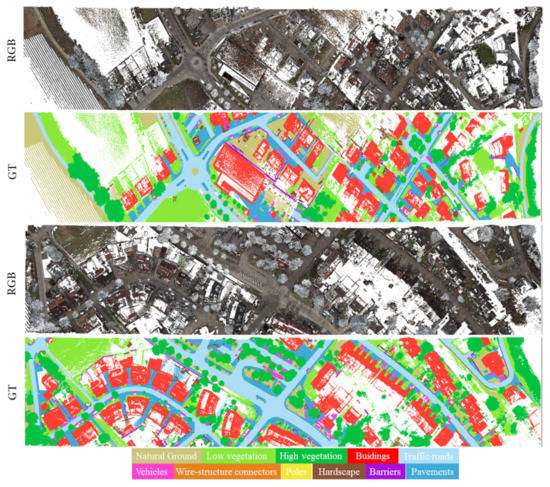
Figure 3.
Examples of the occurring classes of Munzingen dataset. RGB: part of dataset with RGB representation. GT: ground truths—different category labels show in individual colors.
- (0)
- Unclassified: scanning reflections and classes including too few points, i.e. persons and bikes;
- (1)
- Natural ground: natural ground, terrain and grass;
- (2)
- Low vegetation: flowers, shrubs and small bushes;
- (3)
- High vegetation: trees and large bushes higher than 2 m;
- (4)
- Buildings: commercial and residential buildings (our dataset contained no industrial buildings);
- (5)
- Traffic roads: main roads, minor streets and highways;
- (6)
- Wire-structure connectors: power lines and utility lines;
- (7)
- Vehicles: cars, lorries and trucks;
- (8)
- Poles;
- (9)
- Hardscape: a cluttered class, including sculptures, stone statues and fountains;
- (10)
- Barriers: walls, fences and barriers; and
- (11)
- Pavements: footpaths, alleys and cycle paths.
We also designed a category as a cluttered class that contains some classes, such as greenhouses (for plants), wood structures, persons and bikes. If the classes include too few points, the algorithms may not learn features. In addition, the category is not important for our aim; for instance, persons were initially considered to avoid being captured in our dataset. Unclassified points were, thus, labeled with a number 0 class and left in the scene with regard to cohesion.
3.3. Data of Train/Validation/Test Splitting
The training of a DNN is performed in epochs, which are defined as one complete pass through a training dataset. To assess whether a DNN is starting to cause curve-fitting on training data, the DNN is evaluated using a validation dataset after each epoch. To obtain an independent assessment of the model accuracy, a model has to be evaluated with separate test data. Prior to model training, we merged the separate 766 .las files of the investigating area to six tiles, then randomly sampled one tile of the dataset as independent test data.
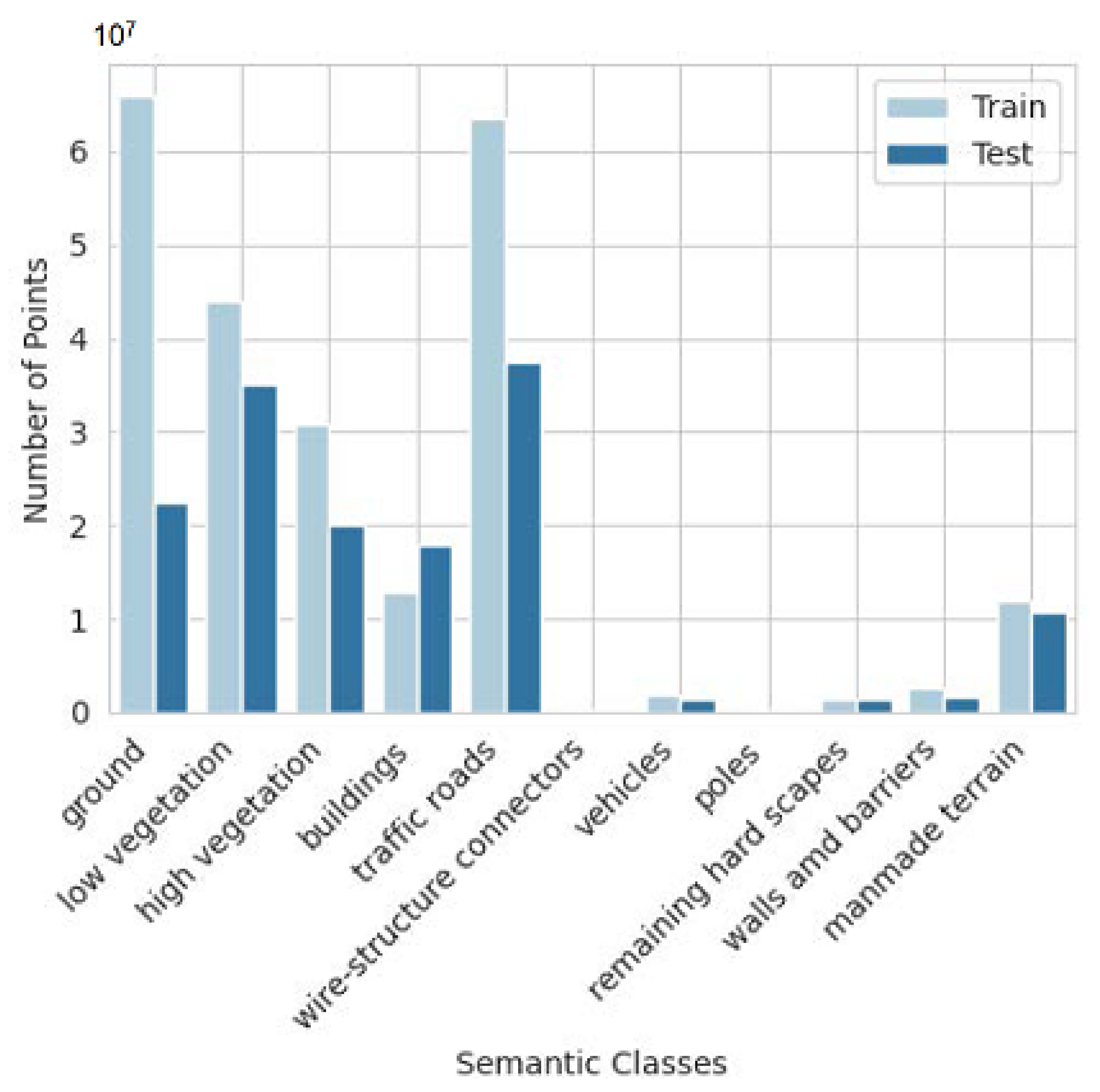
Additionally, with the same scheme as for the test dataset, we randomly select four tiles for model training and one tile for model validation. Figure 4 shows the point clouds distributions of individual categories in both training and test sets. We can see that the categories with most samples are natural ground, low vegetation, high vegetation, buildings and traffic roads. This indicates that the class distribution is very unbalanced. This might be a challenge for all the existing segmentation algorithms.

Figure 4.
The number of points across different object categories in our Munzingen dataset.
3.4. End-to-End Deep Learning Applied to Urban Furniture Segmentation
For urban furniture mapping, we adapted the RandLA-Net architecture [7] by optimizing four different losses during training. Figure 5 illustrates the ARandLA-Net architecture. The ARandLA-Net consists of a standard encoder-decoder architecture with skip connections. Given a large-scale point cloud, each point feature set of our dataset is represented by its 3D coordinates (x-y-z values) and RGB color information. Four encoding layers are applied in the network to step-by-step reduce the size of the point clouds and increase the feature dimensions of each point.
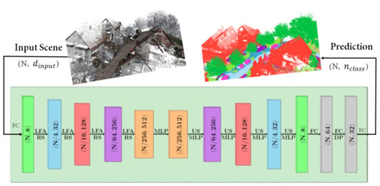
Figure 5.
ARandLA-Net architecture (adapted from [7]) for the urban scene segmentation. This scheme illustrates how the merged Munzingen point clouds tiles are analyzed. The values in the boxes (N, D) depict the number of points and feature dimension. Given an input point cloud, a shared multi-layer perceptron (MLP) layer is applied to extract point-wise features. Then, by employing local feature aggregation (LFA), random sampling (RS), up-sampling (US) and MLP, we used four encoding and decoding layers to learn features for each point cloud. Lastly, three fully connected (FC) layers and one dropout (DP) layer were adapted to output the predicted labels for point clouds.
In each encoding layer, we implemented random sampling and local feature aggregation strategies, to decrease the point density and retain prominent features, respectively. In particular, the point cloud is downsampled by five steps () with one quarter points being retained after each layer. Yet, the per-point feature dimension is constantly raised (for example ) in each layer to preserve more information of complex local structures.
After the encoding processing, four decoding layers were used. We applied the K—nearest neighbors () algorithm in each decoding layer for efficiency, which is based on the point-wise Euclidean distances. By a nearest-neighbor interpolation, the informative point feature set was then upsampled. Subsequently, we stacked the upsampled feature maps with the in-between feature maps composed of previous encoding layers with a skip connection as a standard dilated residual block. The adjusted features were then given to a shared MLP followed by softmax for further concatenating feature maps.
After three shared fully connected layers and a dropout layer, the final class prediction of the respective point is output with a size of , where is the number of classes.
Due to the extremely unbalanced distribution of urban furniture (see Figure 4)—for example, the wire-structure connectors and poles consist of fewer points than traffic roads or natural ground, in addition to the categories of vehicles and barriers as well as hardscape, this makes the network more biased in relation to the classes that appear more in the training data and, therefore, results in relatively poor network performance.
The most probable solution is to apply more sophisticated loss functions. Thereby, we evaluated the effectiveness of four off-the-shelf loss functions during model training, as follows: cross-entropy (CE), weighted cross-entropy with inverse frequency loss (WCE) [21] or with inverse square root frequency loss (WCES) [35] and a combination of WCES and Lovász-Softmax loss (WCESL) [36].
We take an example of poles and wire structure connectors—although they are important categories for the urban management, they appear in much fewer points compared to traffic roads or vegetation in the real city scenarios. This makes the network more biased toward the classes that emerge more in the training data and, thus, yield significantly poorer network performance.
We first define the CE loss as follows:
where p is the number of points, each point p of a given input data has to be classified into an object class . represents the ground truth class of point i, and holds the network probability estimated from the ground truth probability of point i. Secondly, the WCE loss is formulated as:
where and are the true and predicted labels and represents the frequency, for instance the number of points of the category. Thirdly, we also calculate the WCES loss, of the form:
Inspired by [21,36], we also combined the WCES and the Lovász-Softmax loss (Lovász) within the learning procedure to optimize the IoU score, i.e., the Jaccard index. The Lovász is defined as follows:
where is the class number, represents the Lovász extension of the Jaccard index, and and stand for the predicted network probability and ground truth label of point i for the class c, respectively. To enhance the segmentation accuracy, we then formulate the adopted loss function by a combination of the WCES and the Lovász as: .
For better model generalization, random data augmentation was implemented during model training. This augmentation includes applying random vertical flips of the training dataset and randomly adding noise (0.001) of the x-y-z coordinate of input point clouds as well as arbitrarily changing the brightness (80%) and contrast (80%) values of the input points. To investigate whether and how the geometrical and color information impact the final segmentation outputs, we also evaluated the performance by training the model with only 3D coordinate information and both geometry and RGB color information.
Nevertheless, models were trained for 100 epochs with batch sizes of 4 and 14 during training and validation plus the test, respectively. Finally, the epoch with the highest mean Intersection-over-Union () score from the validation dataset was reserved as the final model.
3.5. Evaluation
For the evaluation metrics of the segmentation, we followed the existing point clouds benchmarks [3,10,37,38] to assess the quantitative performance of our approach by the consistency between the predicted results and the ground truth dataset (such as the reference dataset). The predicted results of semantic segmentation by using our approach were compared with the manually segmented reference dataset pointwise. As our task was semantic segmentation, we focused on the correctness of the boundaries of each segment instead of the clustering performance.
It is difficult to obtain the proper positions of points belonging to boundaries. Thus, we adopted the strategy applied by [39,40,41] in the evaluation procedure. As stated in this strategy, correspondence can be found between a pair of segments, including one from the predicted results and another from the ground truth data. The number of true positive (), true negative (), false positive () and false negative () points calculated from the pair were further investigated.
To evaluate our results, we used the overall accuracy (OA), mean accuracy (mean Acc) and the Jaccard index, also referred to as the Intersection-over-Union () averaged over all classes. The evaluation measure for class i is defined as Equations (5)–(9). With these criteria, we can easily conclude whether a prediction is correctly segmented or not as stated by statistical values rather than comparing geometric boundaries in a sophisticated way.
We first define the evaluation of measurement per class i, of the form:
For the multilabel Munzingen dataset, the principle evaluation criterion is the averaged Jaccard index across all eleven classes without the unclassified category, yielding the mIoU as:
We also report and the mean Acc as supplementary criteria. The measure of can be tricky when examining a data set with a skewed class distribution. High accuracy can not be assumed to be because of good results across all classes, as it could be due to overfitting. Yet, we report it for consistency with other point cloud benchmarks. The can be calculated directly from:
where C is the overall number of categories; i is the ith ground-truth label in C; , , and stand for the number of points of true positives, true negatives, false positives, and false negatives of the output results, respectively. Furthermore, the accuracy for each class i is defined by:
The mean accuracy is, thus,
3.6. Implementation
The grid size for downsampling varied from 4 to 20 cm, and the random downsampling ratio was . We sampled a fixed density number of 4096 input points. The adaptive moment estimation (Adam) optimizer [42] was applied with default parameters. The initial learning rate was set at 1 × 10 and decayed by 5% after each epoch, the number of maximum epochs was set to 100, and the number of nearest points K equaled between 20 and 35. For a structured and more manageable flow of information during training, the network divided the Munzingen dataset into a total of four batches during training, and 16 batches during validation and testing. In particular, all raw point clouds were fed into the adapted network to gain the per-point prediction without any extra interpolation. The training of the DNN model was conducted on a CUDA-compatible NVIDIA GPU (TITAN RTX, 24 GB RAM) with the cuDNN library [43].
4. Results
To explore the optimal input data configuration for our DNN, we evaluated different sampling and partitioning of the raw point clouds. The aim was to achieve outstanding results with computational efficiency. The best performing model was trained with x-y-z coordinates plus RGB data and a simple combined strategy of grid sampling plus density-consistent block partition. Table 2 presents the mIoU score and OA score obtained after training the network with two different input preparation steps.

Table 2.
The effects of two different input preparation steps based on ARandLA-Net.
A down-sampling grid size of 0.2 m achieved the best model performance with the mIoU score of 54.4% and OA score of 83.9% (Table 3). Class-specific IoU-scores were the highest for high vegetation (
86.7%), vehicles (75.7%), buildings (73.9%) and traffic roads (63.2%). Furthermore, these IoU scores differed between models with different sub-sampling grids, especially for some dominant classes (i.e., natural ground and high vegetation) and some underrepresented categories (i.e., wire-structure connectors and hardscape), on which larger grid sizes resulted in higher IoU-scores.

Table 3.
Performance evaluation of the ARandLA-Net with varying sub-sampling grid sizes for the individual semantic categories on the Freiburg Munzingen dataset. Semantic segmentation IoU scores are shown per class. We also give the mIoU, OA, and mean accuracy scores across all categories.
However, the results went the opposite way for the categories of barriers and traffic roads. Our understanding of this phenomenon is that the observed local structures (by considering neighboring geometries and corresponded receptive fields) were especially important for these specific classes. Moreover, we notice that larger grid sizes led to a better validation accuracy.
Only taking x-y-z coordinates as input features for the model resulted in a mean IoU score reduction from 54.0% to 50.7% and overall accuracy from 84.1% to 83.8% (Table 4). We further compared our best models based on ARandLA-Net trained on the training scenes of Munzingen city center and then tested on scenes from the Munzingen countryside (Table 5). The mIoU scores slightly dropped in both types of input point clouds (x-y-z plus RGB and only x-y-z). The classes of poles and pavements obtained the worst IoU scores when taking only x-y-z values as inputs.

Table 4.
The effects of different types of input point clouds based on ARandLA-Net.

Table 5.
Comparison of OA, mIoU and per-class IoU on the test set for scenes in the countryside (using the best performing model trained with different types of input point clouds from the City Center).
Figure 6a depicts the network obtaining around 4% mIoU scores when restricted to 20 of neighbors query. The use of advanced loss functions compensated for the imbalanced dataset (Table 6). The best mIoU score raised up to 4%. When it comes to the performance of each individual category, combining the weighted cross-entropy loss with inverse square root frequency (WCES) performed the best in five out of eleven categories.
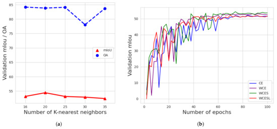
Figure 6.
Experimental results on the Freiburg Munzingen validation set. (a) Evolution of the validation mIoU and OA scores with different choices of K-nearest neighbor based queries. (b) Validation of the mIoU during model training with various advanced loss functions for an equal duration of 100 epochs.

Table 6.
Performance evaluation of the ARandLA-Net with different loss functions for the individual semantic categories on the Freiburg Munzingen dataset. Semantic segmentation IoU scores are shown per class. Additionally, we give the mIoU and OA across all categories.
WCES obtained comparable results with the other approaches in most of these remaining five categories (i.e., high vegetation, low vegetation and barriers). For the classes of poles and wire-structure connectors, the network trained with WCES loss achieved significant improvements in IoU scores of up to 20% and 10%, respectively. In Figure 6b, it can be seen that the mIoU scores of validation begin to be stable from 80 epochs.
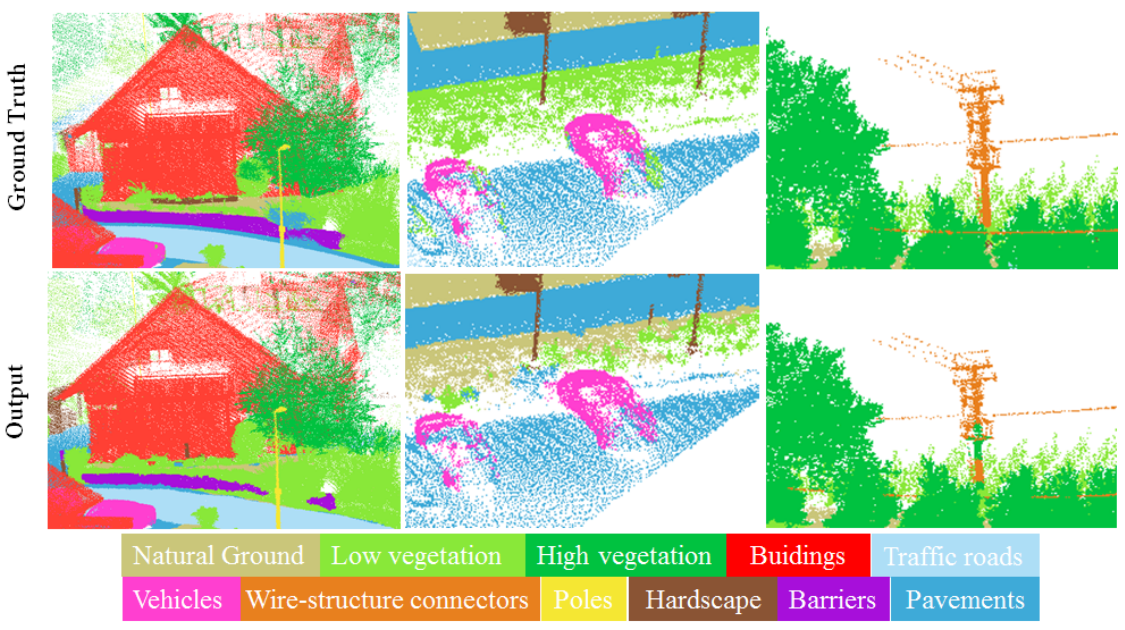
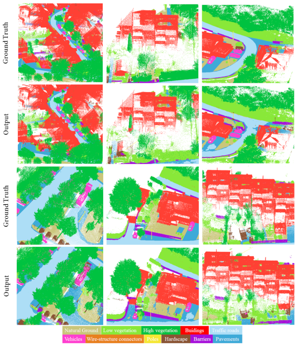
Figure 7 demonstrates the qualitative results of semantic segmentation on the Freiburg Munzingen Dataset. We can see that trees and bushes close to buildings were well-segmented, whereas our network was unable to differentiate a fence from a bush perfectly. This could be due to bushes or vines, for example creepers, growing around or entangling fences. Actual examples of this sort of incompleteness caused by vegetative occlusion can be readily observed alongside streets in German cities. Furthermore, our network detected poles and wire-structure connectors correctly in most cases despite their low density. Moreover, cars were properly predicted despite corruption due to missing points and uneven density.
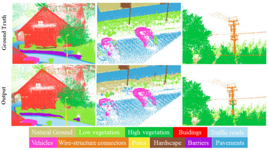
Figure 7.
Qualitative results of semantic segmentation on the Freiburg Munzingen Dataset. The top row represents the ground-truth. The bottom row is the output semantic segmentation results.
We applied the best training model (i.e., ARandLA-Net trained with x-y-z coordinates and RGB with a subsampling grid size of 0.2 m) to a MLS-scene that had not been used for training (Figure 8). Some abundant classes, such as natural ground, high vegetation and buildings, were well predicted; however, the model struggled with underrepresented classes—especially hardscape and barriers.
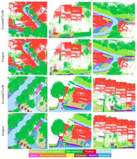
Figure 8.
Predictions of a trained ARandLA-Net in a 0.2 m subsampling grid size. For visualization purposes, segmented object points are projected back to the perspective of 2D representation. The ground-truth segmentations are given in the first and third rows, while the prediction outputs are shown in the second and fourth rows. Classes that do not show in the reference data are grouped in the category “unclassifed”.
5. Discussion
5.1. Data Preparation
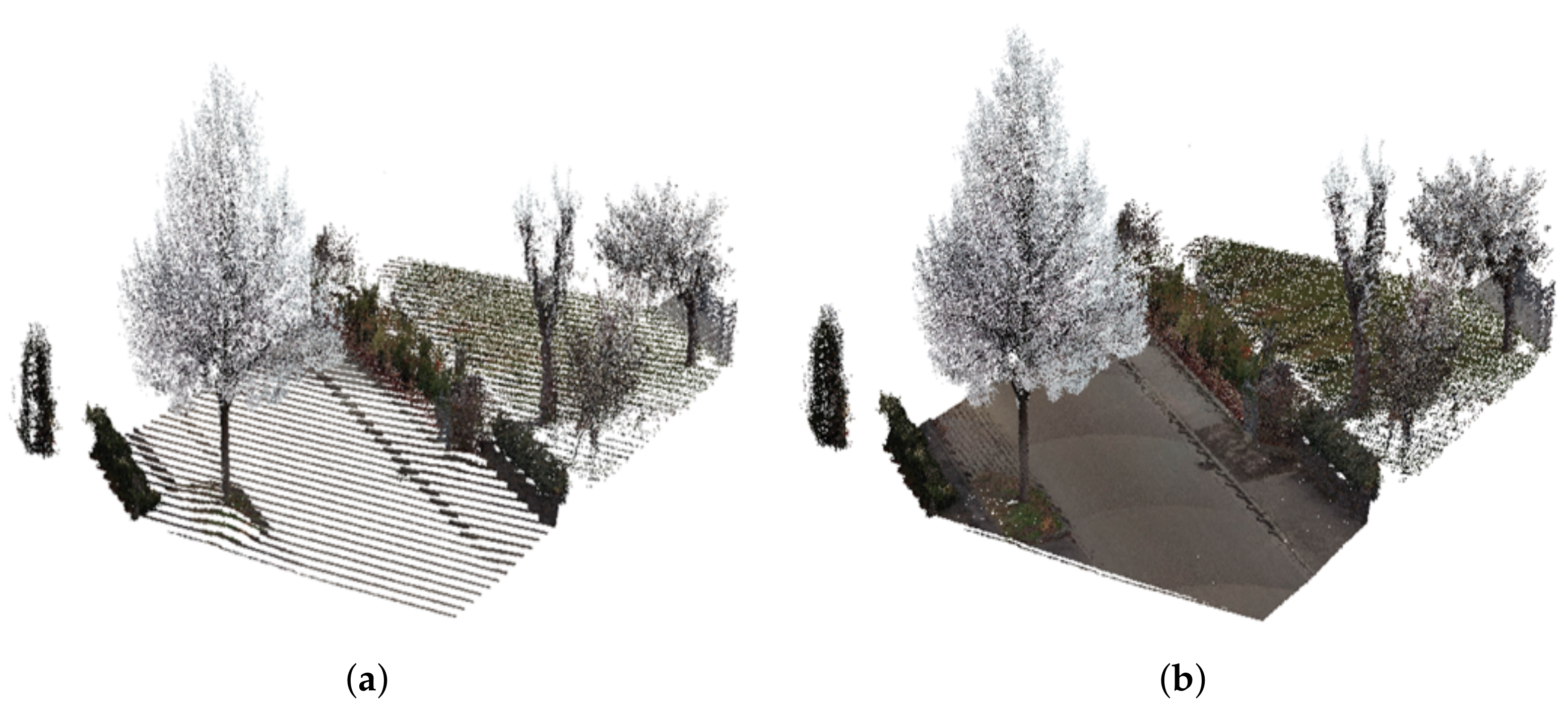
As the x-y coordinates of our original dataset are stored in universal transverse mercator (UTM) format, the y coordinate coordinate exceeds the maximum number of decimal digits in type during directly loading and processing the coordinates (i.e., if using the not type). Figure 9a depicts an example of the issue of loss of detail and incorrect geometrical features. Although we can use the type, why not use a small floating-point format like the single float type? In other words, there is a performance benefit. Compared to storing 64-bit (double float, or FP64) floating-point, lower precision 32-bit (single float, or FP32) floating-point reduces the memory usage of the neural network allowing the training and deployment of larger networks. The single-precision arithmetic had twice the throughput of double-precision arithmetic on the NVIDIA TITAN RTX. Moreover, FP32 data transfers took less time than FP64 transfers. Therefore, we set a UTM_OFFSET value (402,000.0 m, 5,313,800.0 m) to subtract from the plane (x, y) to all the raw coordinates to reduce the number of digits, resulting in Figure 9b.

Figure 9.
Example of the UTM format issue during the subsampling operation: both point clouds in RGB color are subsampled to a grid size of 6 cm. (a) Without offset. (b) With offset.
5.2. Point Clouds Sampling
Processing large-scale point clouds is a challenging task due to the limited memory of GPUs. Thus, the original data is always sampled to a specified size in order to be processed in terms of the balance of computational efficiency and segmentation accuracy. There are many ways to sample the point cloud, for example state-of-the-art methods [24,25,29,44,45,46,47].
The original RandLA-Net uses random sampling to reduce the raw point clouds as it has high efficiency for computation and does not request extra computational memory. Inspired by KPConv [29], the grid sampling technique also offers a way to significantly reduce the number of points. We evaluate both random downsampling and grid downsampling strategies combined with density-consistent block partition on the ARandLA-Net.
Table 2 illustrates the semantic segmentation scores of these two different data partition schemes. In addition, Table 3 shows the performance using different sub-sampling grid sizes to predict the individual semantic classes on the Freiburg Munzingen dataset. It can be seen that the combination of grid downsampling and a set of individual input points of constant density achieved slightly higher mIoU scores than random downsampling. For most of the well-presented classes, the subsampling grid size had an outstanding effect on the model performance. Whereas, for underrepresented classes, a smaller grid size could be a negative factor.
5.3. Class-Balanced Loss Function
Our results show that varying loss functions further led to a higher validation mIoU, in contrast to the original training with the CE, especially for the rare categories represented by a low number of points. The WCES resulted in the highest increment in the mIoU scores because the Jaccard index was directly optimized. We obtained the best mIoU score of 54.4% compared to the other three advanced loss functions. The WCESL loss and the WCES loss gained similar mIoU scores of 52.4% and 52.2%, respectively. The CE loss had the lowest mIoU score (50.7%). We observed, however, that employing different loss functions did not improve the model accuracies for most of the classes, although we achieved the highest overall accuracy score of 84.1%.
The classes hardscape and barriers contained relatively more points than poles and wire-structure connectors, yet did not contribute toward the model performance. Our understanding of this phenomenon is that it has a large variety of possible object shapes, for example street sculptures, which belong to the hardscape class, might show different sizes or heights. It also has only a few training and test samples. Accordingly, there still exist significant performance gaps between individual classes.
5.4. Appearance Information
Adding RGB information as input features to the network clearly increased the model performance for most of the classes. This result is in agreement with the intuition that the presence of RGB information of point clouds is beneficial because it offers additional information as complementary features for the network training to obtain better accuracy of segmentation. The reason, therefore, is that several urban objects (such as traffic roads, pavements and natural ground) are essentially impossible to differ from one another if only geometry is served as an input feature. The color features can help differentiate between these similar geometric categories having different semantics.
In addition, the test results of Table 5 indicate that the model with additional color information performed better than that with only x-y-z values. We note that the semantic segmentation performance of buildings was slightly better than that of the wired-structure connectors. These findings underline the key role that unbalanced class distribution can play in hindering model generalization, as the model tended to be dominated by some categories, whilst the robust features of some other classes failed to be learned and were under-represented.
On the other hand, we notice that Shellnet [32] obtained notably good results, although only x-y-z coordinates were used. This may be linked with the fact that the network overfit the RGB features and did not succeed in learning robust geometric features, and this led to unsatisfactory results. In addition, some algorithms that mainly depend on geometric information can lead, in practice, to better performance without the inclusion of appearance information, such as SPGraph [30], which relies on the geometrical partition.
In most cases, the color information is a considerable presence that can enhance the accuracy of semantic segmentation in the large-scale urban scene. The Dales dataset [37] and the Sensat dataset [38] also highlight the advantage of applying RGB information in model training.
5.5. Reference Data
Our reference data is derived through manual labeling of point clouds. To minimize errors during labeling, we cross-checked the annotation agreement among different labelers. For the Freiburg Munzingen data, a number of reasons suggest that no other method is applicable for obtaining reference data, especially with regard to deep learning: (i) The acquisition of in situ data of the required amount representing real-world scene is cost-prohibitive, time-consuming and labor-intensive and, therefore, might not be easy to achieve. (ii) Some categories are not common to see in other MLS benchmarks, such as wire-structure connectors and barriers.
The wire-structure connectors are illustrated similarly as utility lines in our dataset. These utility lines are usually thin, linear objects that are difficult to classify, especially when they overlap with high vegetation or poles and are close to houses and buildings. The class of barriers includes walls and various obstacles in vertical structures, which makes in situ data difficult to identify. In addition, traffic roads and pavements are two categories in the dataset. In some areas, the traffic roads and sidewalks show homogeneous geometry and surfaces. Such cases, therefore, increase the challenge of segmentation.
6. Conclusions
In this work, we introduced a new large-scene point clouds dataset with point-wise semantic labeled annotations that represents a typical urban scene in central Europe. It consists of about 390 million dense points and 11 semantic categories. We further assessed the potential of a DL-based semantic segmentation approach on MLS prototype point clouds for urban scenarios.
DL-based urban objects mapping was first evaluated with different sampling strategies, incorporating varying partition schemes. The sampling technique had a positive influence on the segmentation accuracy. By combining grid sampling and density-consistent block partition for the data preparation, the total number of points was efficiently and robustly reduced and then fed into the network, thereby, accelerating the application over a large-scale point cloud dataset. This motivated us to further investigate more effective approaches for data preparation. Our findings highlight the advantage of color information for segmentation accuracy. The advancement of LiDAR sensors, the development of intelligent systems and the increasing accessibility of high-quality 3D point cloud data, suggest that RGB is acquired during MLS mapping.
The impact of skewed class distribution should be carefully considered, however. Our study demonstrates the potential of employing class-balanced loss functions and, thus, provides a promising improvement in accuracy, especially for the categories with less abundant points but distinct classes, in the context of semantic segmentation in urban scenes. The use of WCES loss achieved the best result of 54.4% in terms of the mIoU score. However, there is still scope to improve the segmentation performance, especially for the categories of hardscape and barriers. We hope this study will contribute to advancing the research of smart cities.
Author Contributions
Conceptualization, Y.Z.; methodology, Y.Z.; software, Y.Z. and H.W.; validation, Y.Z. and B.K.; formal analysis, Y.Z.; investigation, Y.Z. and H.W.; resources, Y.Z., H.W. and B.K.; data curation, Y.Z.; writing—original draft preparation, Y.Z.; writing—review and editing, Y.Z., H.W. and B.K.; visualization, Y.Z.; supervision, H.W. and B.K.; project administration, B.K.; funding acquisition, Y.Z. and B.K. All authors have read and agreed to the published version of the manuscript.
Funding
This study was funded by the China Scholarship Council (CSC) and partially supported by the Sichuan Ministry of Education, China.
Institutional Review Board Statement
Not applicable.
Informed Consent Statement
Not applicable.
Data Availability Statement
The sample data used in this study can be made available with the permission of the Vermessungsamt of Freiburg.
Acknowledgments
We would like to thank the editors and anonymous reviewers for their constructive comments and suggestions that helped to improve this manuscript. Many thanks to Qingyong Hu, Ben Wilheim, and Xiaohui Song for their valuable comments and discussions. We thank Jan Herrmann and Ines Gavrilut for the proofreading. Special thanks to Richard McNeill for the further proofreading as a native English speaker and Houssem Bendmid for assistance in the point cloud annotation. We also thank for their support the Chair of Remote Sensing and Landscape Information Systems, University of Freiburg. Finally, we thank the Vermessungsamt of the city of Freiburg for providing the point cloud survey data. The article processing charge was funded by the Baden-Wuerttemberg Ministry of Science, Research and Art and the University of Freiburg in the funding program Open Access.
Conflicts of Interest
The authors declare that they have no known competing financial interest or personal relationships that could have appeared to influence the work reported in this study.
Abbreviations
The following abbreviations are used in this manuscript:
| ALS | Airborne LiDAR scanning |
| ARandLA-Net | Adapted RandLA-Net |
| CAD | Computer-Aided design |
| CE | Cross-Entropy |
| CNNs | Convolutional neural networks |
| DL | Deep learning |
| DP | Dropout |
| DNN | Deep neural network |
| FC | Fully connected |
| FP | False positive |
| FN | False negative |
| GPS | Global positioning system |
| GT | Ground truths |
| IoU | Intersection-over-Union |
| LFA | Local feature aggregation |
| LiDAR | Light detection and ranging |
| Lovász | Lovász-Softmax |
| mean Acc | Mean accuracy |
| mean IoU | Mean Intersection-over-Union |
| MLS | Mobile laser scanning |
| MLPs | Multi-Layer Perceptrons |
| NIR | Near infrared |
| OA | Overall accuracy |
| RF | Random forest |
| RGB | Red–green–blue |
| RNN | Recurrent Neural Network |
| RS | Random sampling |
| SVM | Support vector machine |
| TLS | Terrestrial LiDAR scanning |
| TN | True negative |
| TP | True positive |
| ULS | Unmanned LiDAR scanning |
| UP | Up-Sampling |
| UTM | Universal transverse mercator |
| WCE | Weighted cross-entropy with inverse frequency |
| WCES | Weighted cross-entropy with inverse square root frequency |
| WCESL | A combination of the WCES and the Lovász |
| 2D | Two-Dimensional |
| 3D | Three-Dimensional |
References
- Xu, Y.; Boerner, R.; Yao, W.; Hoegner, L.; Stilla, U. Pairwise coarse registration of point clouds in urban scenes using voxel-based 4-planes congruent sets. ISPRS J. Photogramm. Remote Sens. 2019, 151, 106–123. [Google Scholar] [CrossRef]
- Luo, H.; Khoshelham, K.; Fang, L.; Chen, C. Unsupervised scene adaptation for semantic segmentation of urban mobile laser scanning point clouds. ISPRS J. Photogramm. Remote Sens. 2020, 169, 253–267. [Google Scholar] [CrossRef]
- Hackel, T.; Savinov, N.; Ladicky, L.; Wegner, J.D.; Schindler, K.; Pollefeys, M. SEMANTIC3D.NET: A new large-scale point cloud classification benchmark. ISPRS Ann. Photogramm. Remote Sens. Spat. Inf. Sci. 2017, IV-1–W1, 91–98. [Google Scholar] [CrossRef] [Green Version]
- Zai, D.; Li, J.; Guo, Y.; Cheng, M.; Huang, P.; Cao, X.; Wang, C. Pairwise registration of TLS point clouds using covariance descriptors and a non-cooperative game. ISPRS J. Photogramm. Remote Sens. 2017, 134, 15–29. [Google Scholar] [CrossRef]
- Theiler, P.; Wegner, J.; Schindler, K. Keypoint-based 4-Points Congruent Sets—Automated marker-less registration of laser scans. ISPRS J. Photogramm. Remote Sens. 2014, 96, 149–163. [Google Scholar] [CrossRef]
- Theiler, P.; Wegner, J.; Schindler, K. Globally consistent registration of terrestrial laser scans via graph optimization. ISPRS J. Photogramm. Remote Sens. 2015, 109, 126–138. [Google Scholar] [CrossRef]
- Hu, Q.; Yang, B.; Xie, L.; Rosa, S.; Guo, Y.; Wang, Z.; Trigoni, N.; Markham, A. RandLA-Net: Efficient Semantic Segmentation of Large-Scale Point Clouds. In Proceedings of the IEEE Conference on Computer Vision and Pattern Recognition, Long Beach, CA, USA, 16–20 June 2019. [Google Scholar]
- Munoz, D.; Bagnell, J.A.; Vandapel, N.; Hebert, M. Contextual Classification with Functional Max-Margin Markov Networks. In Proceedings of the IEEE Conference on Computer Vision and Pattern Recognition (CVPR), Miami, FL, USA, 20–25 June 2009. [Google Scholar]
- Roynard, X.; Deschaud, J.E.; Goulette, F. Paris-Lille-3D: A large and high-quality ground-truth urban point cloud dataset for automatic segmentation and classification. Int. J. Robot. Res. 2017, 37, 545–557. [Google Scholar] [CrossRef] [Green Version]
- Tan, W.; Qin, N.; Ma, L.; Li, Y.; Du, J.; Cai, G.; Yang, K.; Li, J. Toronto-3D: A large-scale mobile lidar dataset for semantic segmentation of urban roadways. In Proceedings of the IEEE/CVF Conference on Computer Vision and Pattern Recognition Workshops, Seattle, WA, USA, 14–19 June 2020; pp. 202–203. [Google Scholar]
- Guo, Y.; Wang, H.; Hu, Q.; Liu, H.; Liu, L.; Bennamoun, M. Deep learning for 3D point clouds: A survey. IEEE Trans. Pattern Anal. Mach. Intell. 2020, in press. [Google Scholar] [CrossRef] [PubMed]
- Griffiths, D.; Boehm, J. A Review on Deep Learning Techniques for 3D Sensed Data Classification. Remote Sens. 2019, 11, 1499. [Google Scholar] [CrossRef] [Green Version]
- Graham, B.; Engelcke, M.; van der Maaten, L. 3D Semantic Segmentation With Submanifold Sparse Convolutional Networks. In Proceedings of the IEEE Conference on Computer Vision and Pattern Recognition (CVPR), Lake City, UT, USA, 18–22 June 2018. [Google Scholar]
- Choy, C.; Gwak, J.; Savarese, S. 4D Spatio-Temporal ConvNets: Minkowski Convolutional Neural Networks. In Proceedings of the IEEE Conference on Computer Vision and Pattern Recognition, Long Beach, CA, USA, 16–20 June 2019; pp. 3075–3084. [Google Scholar]
- Le, T.; Duan, Y. PointGrid: A Deep Network for 3D Shape Understanding. In Proceedings of the IEEE Conference on Computer Vision and Pattern Recognition (CVPR), Lake City, UT, USA, 18–22 June 2018; pp. 9204–9214. [Google Scholar] [CrossRef]
- Liu, Z.; Tang, H.; Lin, Y.; Han, S. Point-Voxel CNN for Efficient 3D Deep Learning. In Proceedings of the Advances in Neural Information Processing Systems, Vancouver, BC, Canada, 8–14 December 2019. [Google Scholar]
- Meng, H.Y.; Gao, L.; Lai, Y.K.; Manocha, D. VV-Net: Voxel VAE Net With Group Convolutions for Point Cloud Segmentation. In Proceedings of the IEEE Conference on Computer Vision and Pattern Recognition, Long Beach, CA, USA, 16–20 June 2019; pp. 8499–8507. [Google Scholar] [CrossRef] [Green Version]
- Zhang, Y.; Zhou, Z.; David, P.; Yue, X.; Xi, Z.; Gong, B.; Foroosh, H. PolarNet: An Improved Grid Representation for Online LiDAR Point Clouds Semantic Segmentation. In Proceedings of the IEEE/CVF Conference on Computer Vision and Pattern Recognition (CVPR), Seattle, WA, USA, 14–19 June 2020. [Google Scholar]
- Xie, Y.; Tian, J.; Zhu, X.X. Linking Points With Labels in 3D: A Review of Point Cloud Semantic Segmentation. IEEE Geosci. Remote Sens. Mag. 2020, 8, 38–59. [Google Scholar] [CrossRef] [Green Version]
- Lyu, Y.; Huang, X.; Zhang, Z. Learning to Segment 3D Point Clouds in 2D Image Space. In Proceedings of the IEEE/CVF Conference on Computer Vision and Pattern Recognition (CVPR), Seattle, WA, USA, 14–19 June 2020; pp. 12255–12264. [Google Scholar]
- Cortinhal, T.; Tzelepis, G.; Aksoy, E.E. SalsaNext: Fast, Uncertainty-aware Semantic Segmentation of LiDAR Point Clouds for Autonomous Driving. arXiv 2020, arXiv:cs.CV/2003.03653. [Google Scholar]
- Xu, C.; Wu, B.; Wang, Z.; Zhan, W.; Vajda, P.; Keutzer, K.; Tomizuka, M. Squeezesegv3: Spatially-adaptive convolution for efficient point-cloud segmentation. In Proceedings of the European Conference on Computer Vision, Glasgow, UK, 23–28 August 2020; Springer: Cham, Switzerland, 2020; pp. 1–19. [Google Scholar]
- Austin, M.; Delgoshaei, P.; Coelho, M.; Heidarinejad, M. Architecting Smart City Digital Twins: Combined Semantic Model and Machine Learning Approach. J. Manag. Eng. 2020, 36, 04020026. [Google Scholar] [CrossRef]
- Qi, C.R.; Su, H.; Mo, K.; Guibas, L.J. PointNet: Deep Learning on Point Sets for 3D Classification and Segmentation. arXiv 2016, arXiv:1612.00593. [Google Scholar]
- Qi, C.R.; Yi, L.; Su, H.; Guibas, L.J. PointNet++: Deep Hierarchical Feature Learning on Point Sets in a Metric Space. arXiv 2017, arXiv:1706.02413. [Google Scholar]
- Li, Y.; Bu, R.; Sun, M.; Wu, W.; Di, X.; Chen, B. PointCNN: Convolution on Xtransformed points. Adv. Neural Inf. Process. Syst. 2018, 31, 820–830. [Google Scholar]
- Tatarchenko, M.; Park, J.; Koltun, V.; Zhou, Q.Y. Tangent Convolutions for Dense Prediction in 3D. In Proceedings of the IEEE Conference on Computer Vision and Pattern Recognition (CVPR), Lake City, UT, USA, 18–22 June 2018. [Google Scholar]
- Wang, Y.; Sun, Y.; Liu, Z.; Sarma, S.E.; Bronstein, M.M.; Solomon, J.M. Dynamic Graph CNN for Learning on Point Clouds. ACM Trans. Graph. (TOG) 2019, 38, 1–12. [Google Scholar] [CrossRef] [Green Version]
- Thomas, H.; Qi, C.R.; Deschaud, J.E.; Marcotegui, B.; Goulette, F.; Guibas, L.J. KPConv: Flexible and Deformable Convolution for Point Clouds. In Proceedings of the IEEE International Conference on Computer Vision, Seoul, Korea, 27–28 October 2019. [Google Scholar]
- Loic, L.; Martin, S. Large-scale Point Cloud Semantic Segmentation with Superpoint Graphs. In Proceedings of the IEEE Conference on Computer Vision and Pattern Recognition (CVPR), Lake City, UT, USA, 18–22 June 2018. [Google Scholar]
- Huang, Q.; Wang, W.; Neumann, U. Recurrent Slice Networks for 3D Segmentation on Point Clouds. arXiv 2018, arXiv:1802.04402. [Google Scholar]
- Zhang, Z.; Hua, B.S.; Yeung, S.K. ShellNet: Efficient Point Cloud Convolutional Neural Networks using Concentric Shells Statistics. In Proceedings of the IEEE International Conference on Computer Vision, Seoul, Korea, 27–28 October 2019. [Google Scholar]
- Weinacker, H.; Koch, B.; Weinacker, R. TREESVIS: A software system for simultaneous ED-real-time visualisation of DTM, DSM, laser raw data, multispectral data, simple tree and building models. ISPRS J. Photogramm. Remote Sens. 2004, 36, 90–95. [Google Scholar]
- Girardeau-Montaut, D. CloudCompare. Available online: https://www.danielgm.net/cc/ (accessed on 22 June 2021).
- Rosu, R.A.; Schütt, P.; Quenzel, J.; Behnke, S. LatticeNet: Fast point cloud segmentation using permutohedral lattices. In Proceedings of the Robotics: Science and Systems (RSS), Online, 12–16 July 2020. [Google Scholar]
- Berman, M.; Rannen Triki, A.; Blaschko, M.B. The Lovász-Softmax loss: A tractable surrogate for the optimization of the intersection-over-union measure in neural networks. In Proceedings of the IEEE Conference on Computer Vision and Pattern Recognition (CVPR), Lake City, UT, USA, 18–22 June 2018; pp. 4413–4421. [Google Scholar]
- Varney, N.; Asari, V.; Graehling, Q. DALES: A Large-scale Aerial LiDAR Data Set for Semantic Segmentation. In Proceedings of the 2020 IEEE/CVF Conference on Computer Vision and Pattern Recognition Workshops (CVPRW), Seattle, WA, USA, 14–19 June 2020; pp. 717–726. [Google Scholar] [CrossRef]
- Hu, Q.; Yang, B.; Khalid, S.; Xiao, W.; Trigoni, N.; Markham, A. Towards Semantic Segmentation of Urban-Scale 3D Point Clouds: A Dataset, Benchmarks and Challenges. In Proceedings of the IEEE/CVF Conference on Computer Vision and Pattern Recognition, New Orleans, LO, USA, 19–24 June 2021. [Google Scholar]
- Awrangjeb, M.; Fraser, C. Automatic Segmentation of Raw LIDAR Data for Extraction of Building Roofs. Remote Sens. 2014, 6, 3716–3751. [Google Scholar] [CrossRef] [Green Version]
- Vo, A.V.; Truong-Hong, L.; Laefer, D.; Bertolotto, M. Octree-based region growing for point cloud segmentation. ISPRS J. Photogramm. Remote Sens. 2015, 104, 88–100. [Google Scholar] [CrossRef]
- Nurunnabi, A.; Geoff, W.; Belton, D. Outlier Detection and Robust Normal-Curvature Estimation in Mobile Laser Scanning 3D Point Cloud Data. Pattern Recognit. 2015, 48, 1404–1419. [Google Scholar] [CrossRef] [Green Version]
- Kingma, D.; Ba, J. Adam: A Method for Stochastic Optimization. In Proceedings of the International Conference on Learning Representations, Banff, AB, Canada, 14–16 April 2014. [Google Scholar]
- Chetlur, S.; Woolley, C.; Vandermersch, P.; Cohen, J.; Tran, J.; Catanzaro, B.; Shelhamer, E. cuDNN: Efficient Primitives for Deep Learning. arXiv 2014, arXiv:1410.0759. [Google Scholar]
- Lang, I.; Manor, A.; Avidan, S. SampleNet: Differentiable Point Cloud Sampling. In Proceedings of the IEEE/CVF Conference on Computer Vision and Pattern Recognition (CVPR), Seattle, WA, USA, 14–19 June 2020; pp. 7575–7585. [Google Scholar] [CrossRef]
- Dovrat, O.; Lang, I.; Avidan, S. Learning to Sample. In Proceedings of the IEEE Conference on Computer Vision and Pattern Recognition (CVPR), Lake City, UT, USA, 18–22 June 2018. [Google Scholar]
- Xu, Q.; Sun, X.; Wu, C.Y.; Wang, P.; Neumann, U. Grid-GCN for Fast and Scalable Point Cloud Learning. In Proceedings of the IEEE/CVF Conference on Computer Vision and Pattern Recognition (CVPR), Seattle, WA, USA, 14–19 June 2020; pp. 5660–5669. [Google Scholar] [CrossRef]
- Yan, X.; Zheng, C.; Li, Z.; Wang, S.; Cui, S. PointASNL: Robust Point Clouds Processing using Nonlocal Neural Networks with Adaptive Sampling. In Proceedings of the IEEE/CVF Conference on Computer Vision and Pattern Recognition (CVPR), Seattle, WA, USA, 14–19 June 2020. [Google Scholar]
Publisher’s Note: MDPI stays neutral with regard to jurisdictional claims in published maps and institutional affiliations. |
© 2021 by the authors. Licensee MDPI, Basel, Switzerland. This article is an open access article distributed under the terms and conditions of the Creative Commons Attribution (CC BY) license (https://creativecommons.org/licenses/by/4.0/).

