A Novel Method for Fast Positioning of Non-Standardized Ground Control Points in Drone Images

Abstract

Positioning the pixels of ground control points (GCPs) in drone images is an issue of great concern in the field of drone photogrammetry. The current mainstream automatic approaches are based on standardized markers, such as circular coded targets and point coded targets. There is no denying that introducing standardized markers improves the efficiency of positioning GCP pixels. However, the low flexibility leads to some drawbacks, such as the heavy logistical input in placing and maintaining GCP markers. Especially as drone photogrammetry steps into the era of large scenes, the logistical input in maintaining GCP markers becomes much more costly. This paper proposes a novel positioning method applicable for non-standardized GCPs. Firstly, regions of interest (ROIs) are extracted from drone images with stereovision technologies. Secondly, the quality of ROIs is evaluated using image entropy, and then the outliers are filtered by an adjusted boxplot. Thirdly, pixels of interest are searched with a corner detector, and the precise imagery coordinates are obtained by subpixel optimization. Finally, the verification was carried out in an urban scene, and the results show that this method has good applicability to the GCPs on road traffic signs, and the accuracy rate is over 95%.

1. Introduction

Drone photogrammetry is a relatively new technique that has gradually become popular because of its flexibility and cost-efficient data acquisition. It has been applied in many fields, such as construction planning [1], mapping [2], structure monitoring [3] and disaster assessment [4]. In drone photogrammetry, the key to achieving high precision is to establish an accurate correspondence between drone images and the spatial world. Usually, this correspondence is established with the so-called ground control points (GCPs). The spatial coordinates of GCPs are surveyed using geodetic instruments (e.g., GNSS stations) and then attached to the corresponding image pixels. According to the performance evaluation conducted by [5,6,7,8], the precision of drone photogrammetry can reach centimeter-level or even millimeter-level when a set of GCPs are well surveyed and attached. However, if any unexpected error occurs during attaching, the effectiveness of GCPs would decrease significantly. In this regard, the pixel positioning of GCPs is a fundamental and essential aspect of drone photogrammetry.

The traditional approach to detect and extract GCP pixels is via manual operation by photo interpreters. In this way, photo interpreters search for GCP pixels in drone images based on the prior knowledge delivered from survey teams, e.g., in situ pictures or freehand sketching of GCP surroundings. The most striking feature of the traditional approach is that it relies on operators’ skills, which tends to be flexible but time-consuming.

Due to its flexibility, manual operation is prevalent in small-scale projects since they only require a few GCPs and the time cost is acceptable. However, in large-scale projects, the number of images may run into the thousands, and dozens of GCPs may be involved. In this case, manual searching and extracting GCP pixels unfortunately become much more cumbersome. Moreover, even if expert interpreters carry out the operation, errors are still prone to happen, and efficiency cannot be guaranteed. For these reasons, the traditional approach has become less practical in the era of large-scene drone photogrammetry.

Automatic approaches can meet the need for efficiency and accuracy and may replace the traditional approach in the foreseeable future. In the last decades, many attempts were made and different automatic approaches have been proposed in the literature. Some automatic approaches are designed for standardized GCPs, and others for non-standardized ones. The approaches for standardized GCPs seem to be developed and applied better since the standardization of GCPs greatly reduces the difficulty of constructing image feature detectors. Usually, fiducial markers are preferred as standardized GCPs, such as circular coded targets (CCTs) [9,10,11] and point coded targets (PCTs) [12,13,14]. Besides, non-coded markers such as square tiles are also widely used [15]. In typical practice, such fiducial markers are placed on the ground as GCPs and then surveyed by GNSS stations or total stations. After drone photography, a specific image detector, which identifies fiducial markers by color, shape, texture, or other features, is used to perform automatic detection. With the help of detectors from fiducial schemes, the efficiency of detecting GCPs is highly improved, and quality can also be guaranteed. However, although standardizing GCPs is beneficial, it suffers from a series of pitfalls. On the one hand, much workforce and resources are in demand for placing and maintaining markers. On the other hand, markers are so easily disturbed by animals and vehicles that the GCPs at the disturbed markers often break down for becoming no longer stationary.

Unlike standardized GCPs, the use of non-standardized GCPs requires less logistical input because arbitrary natural objects can serve as GCPs. For example, Joji et al. [16] applied a Hough transform-based approach to multi-look images and automatically extracted the road intersections as GCPs. Purevdorj et al. [17] used an edge detection approach to extract coastline and identified GCPs by line matching. Similarly, Zhang et al. [18] also took coastline corners as GCPs for image correction. Deng et al. [19] worked on corner extraction and proposed an adaptive algorithm which could extract valuable GCPs. Davide et al. [20] selected a general-purpose corner detector, the Harris algorithm, to carry out automated detection so that arbitrary bright isolated objects can serve as GCPs. Template matching is another popular way. For instance, Sina et al. [21,22] took widespread lamp posts as GCPs and utilized template matching to achieve automated searching. Cao et al. [23] presented a template-based method and tried to build a template library for different ground signs. Although the above work achieved fast positioning of non-standardized GCPs in some ways, only limited forms of non-standardized GCPs were considered and provided with solutions. Moreover, there is little consideration of mechanisms to avoid wrong detections in most studies to our best knowledge. Hence, there is a strategic interest in further developing the methods for fast positioning non-standardized GCPs in drone images.

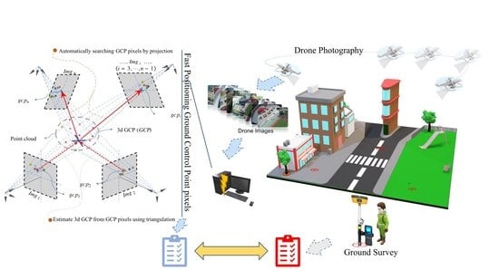
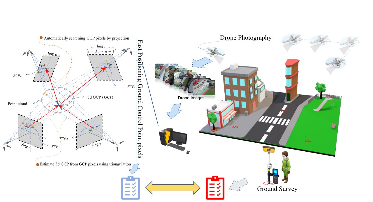
In this paper, a novel method for fast positioning non-standardized GCPs in drone images is presented. In details, it consists of three main parts. Firstly, the relative spatial poses of drone images are recovered with multi-view constraints from feature correspondences, and image regions of interest are extracted through ray projection. Secondly, visibility check and outlier removal are carried out with an adjusted boxplot of edge-based image entropy. Finally, coarse and precise coordinates of the GCP pixels are obtained by corner detection and subpixel optimization. An Olympic sports center was selected for the experimental test, and five different road traffic signs are taken as non-standardized GCPs. The applicability of the proposed method is demonstrated with the processing results.

2. Methodology

Positioning non-standardized GCPs in drone images could be considered a problem of object detection and recognition. It is challenging because there are few consistent similarities between different types of non-standardized GCPs, making it almost impossible to design universe detectors or large-scale template libraries. Furthermore, the image features of non-standardized GCPs are usually not exclusive, which tends to bring trouble when performing identification. To be specific, three problems need to be considered. The first problem to be tackled is detecting and extracting the objects that act as non-standardized GCPs. Secondly, the similarity between GCPs may bring distraction when identifying the objects extracted. The last problem to be addressed is to obtain coordinates of GCP pixels under a satisfactory precision requirement.

Different from the most existing literature, this paper does not tackle the detection problem directly within images but instead takes pixel rays of drone images as a middleware. In this way, search regions are narrowed to the neighborhood near the rays. Moreover, identification information can also be delivered as the rays travel. Then, after detection and extraction, quality evaluation and outliers removal are executed, which screens out negative results from the previous step. Finally, coarse and precise positioning are carried out by corner detection and subpixel optimization, respectively.

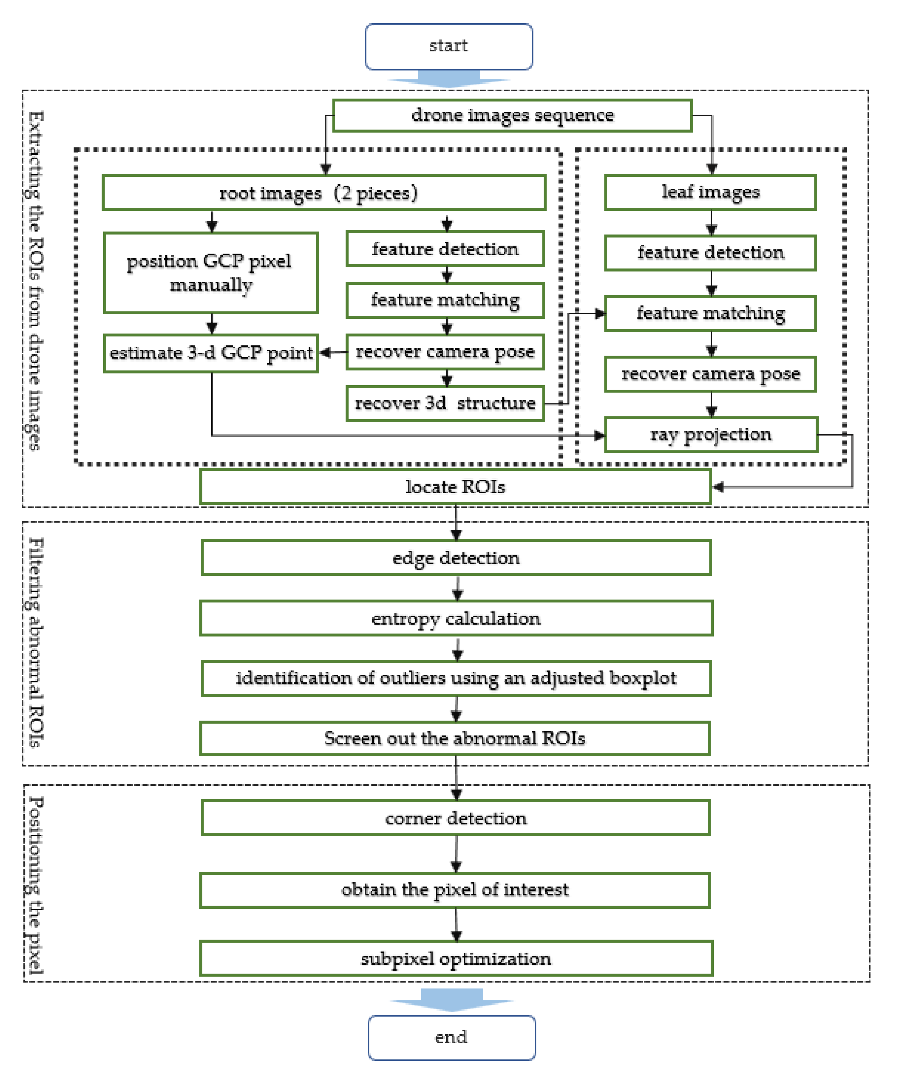
The flowchart of the proposed method is shown in Figure 1, composed of three main processes. These processes have to be carried out in the stated order: (i) the first part (upper zone) is responsible for searching drone images and extracting the regions of interest (ROIs) that contain target GCPs, (ii) the second part (middle zone) is designed to identify and filter the low-quality ROIs to reduce the risk of unexpected errors, and (iii) the third part (lower zone) is responsible for positioning the pixels of the target GCPs in ROIs.

2.1. Extracting the Regions of Interest from Drone Images

The first task consists in extracting the ROIs for target GCPs from drone images. Usually, images are overlapped in a drone photogrammetry practice, which forms a typical multi-view scene. According to stereo vision theory, imagery pixels can be positioned in a multi-view scene by projecting a spatial point. In turn, this spatial point can be estimated by the back-projection of the pixels. Such properties are attractive and worth utilization to help search identical non-standardized GCPs since the projection rays can serve as channels for transferring identification information. Moreover, the ROIs can be located along with the projection rays. The schematic diagram is shown in Figure 2, and it consists of the following four steps:

• Step 1 (Pose recovery of the root images): Take two images containing a target GCP as root images ($Im{g}_1$ , $Im{g}_2$) and the remaining images as leaf images ($Im{g}_i,i=3,4,\cdots ,n$). And, manually position the pixels of the target GCP in the root images as $gc{p}_1$and$gc{p}_2$. Detect features in the root images and match them based on a similarity metric between their descriptors. Camera motions (rotation component $R$ and translation component $t$) of the root images can be computed from the feature correspondences using the epipolar constraint, denoted as ($R_i, t_i ,i=1,2$).
• Step 2 (Reconstruction of the 3d structure): Triangulate the feature correspondences in the root images to reconstruct the spatial points, which compose the 3d structure.
• Step 3 (Pose recovery of the leaf images): Detect features in the leaf images and match their descriptors with the descriptors of the 3d structure. Camera motions of these leaf images can be computed from the correspondences between the 3d structure and the images, denoted as$(R_i, t_i ,i=3,4,\cdots ,n)$ .
• Step 4 (Extraction of the regions of interest): Triangulate the GCP pixels from the root images to estimate spatial coordinates of the target GCP. Then this spatial point is projected onto the leaf images to generate a set of new GCP pixels ($gc{p}_i ,i=3,4,\cdots ,n$ ). The new GCP pixels are regarded as centers of the ROIs.

These four steps are discussed in detail in Section 2.1.1, Section 2.1.2, Section 2.1.3 and Section 2.1.4, respectively. However, it is important to note that some details of the algorithms used may not be expanded since they are well-documented in the literature.

2.1.1. Pose Recovery of the Root Images

The root images ($Im{g}_1$ and $Im{g}_2$) should be selected manually. It worth noting that although the manual operation is involved here, the overall efficiency of the proposed method is still satisfactory since the amount of the root images is scant compared with the remaining hundreds of images. The basic requirement for the root images is that they should cover the same target GCP, i.e., there are identical pixels of a target GCP. Identical GCP pixels imply that many similar image features can be found in the root images. This lays the foundation for recovering the poses of the root images because such similar features can be used to establish feature correspondences and these feature correspondences are applicable for the epipolar constraint. In detail, the processing chain for pose recovery of the root images includes a set of procedures that starts from establishing feature correspondences to estimating the essential matrix and then extracting motions from the essential matrix.

The feature extraction should be precise but also repeatable. Therefore, the popular scale-invariant feature transform (SIFT) algorithm [24] is used. The SIFT algorithm has several advantages, such as robustness, repeatability, accuracy, and distinctiveness. First, key locations are defined as maxima and minima of the Gaussian function difference in scale space. Next, dominant orientations are assigned to the localized key locations. Then, SIFT descriptors robust to local affine distortion are then obtained by considering pixels around the key locations. More details about the algorithm can refer to the study of [24]. With the SIFT algorithm, sufficient salient features are available in the root images ($Im{g}_1$and $Im{g}_2$). These features are located as pixels ($p_1$ and $p_2$) and described as feature descriptors ($de{s}_1 \mathrm{and} de{s}_2$).

After the feature detection, all feature descriptors in $de{s}_1$are compared with those in $de{s}_2$, and Euclidean distances are calculated to quantify similarity. A smaller Euclidean distance stands for the higher similarity between a pair of features. Therefore, each feature pixel in $p_1$ is linked to another in $p_2$ with the closest descriptor, which generates feature correspondences.

Such correspondences are so-called 2d–2d correspondences because pixels are two-dimensional. The main property of these 2d–2d correspondences is that they satisfy the epipolar constraint, formulated as follows:

$${p_2}^{-T}{K_2}^{-T}E{K_1}^{-1}{p}_1=0$$

(1)

where $K_1 \mathrm{and} K_2$are the internal parameter matrices of $Im{g}_1$and$Im{g}_2$respectively.

The so-called essential matrix $E$ describes the geometric relations between $Im{g}_1$ and $Im{g}_2$, which contains the camera motions implicitly. Given $K_1$, $K_2$and $p_1$, $p_2$, the essential matrix $E$ can be computed from 2d–2d correspondences by the eight-point method [25]. Then, after estimating $E$, the rotation and translation parts can be extracted from $E$ using the singular value decomposition (SVD) method [26] as $R$and $t$:

$$\begin{gathered} R=UW\left(\pm \frac{\Pi }{2}\right)V^T, \\ t=UW\left(\pm \frac{\Pi }{2}\right)D{V}^T, \end{gathered}$$

(2)

where $E=UD{V}^T,W\left(\pm \frac{\Pi }{2}\right)=\left[\begin{array}{ccc}0& \pm 1& 0\\ \mp 1& 0& 0\\ 0& 0& 1\end{array}\right]$, and $D=diag\left(1,1,0\right).$ In general, there are four cases for $R$,$t$ pairs, where the correct one can be identified by whether a spatial point is in front of both images.

The obtained $R$ and $t$ are the relative motion components between $Im{g}_1$ and $Im{g}_2$. For global reference, in this paper, the local reference system of $Im{g}_1$ is directly selected as the global reference system. Thus, $R_1=diag\left(1,1,1\right)$,$t_1={\left[0,0,0\right]}^T$,$R_2=R$ and $t_2=t$.

2.1.2. Reconstruction of the 3d Structure

Given the camera motions (also known as external parameters) of images, triangulation is allowed, where rays from identical pixels are back-projected and intersected. In this way, spatial points (3d structure) can be reconstructed from 2d–2d correspondences. The details for triangulation can be found in the literature, so this paper only provides the basic principles.

In a binocular vision system formed by $Im{g}_1$ and $Im{g}_2$, suppose there is a spatial point $P$ and its corresponding feature pixels ($p_1$ and $p_2$). Let $P_1$, $P_2$ be the local spatial coordinates of $P$ in the coordinate system of $Im{g}_1$ and $Im{g}_2$.Then, the following relation can be established:

$$s_2{K_2}^{-1}{p}_2=R{s}_1{K_1}^{-1}{p}_1+t$$

(3)

where $s_1 \mathrm{and} s_2$ are depth factors;$R$ and $t$ are the relative motion components between $Im{g}_1$ and $Im{g}_2$. Let $x_2={K_2}^{-1}{p}_2$ and $x_1={K_1}^{-1}{p}_1$, and then multiplying both sides of Equation (3) by the antisymmetric matrix of $x_2$ yields:

$$\widehat{x_2}{s}_{1}R{x}_1+\widehat{x_2}t=0$$

(4)

Equation (4) has nine degrees of freedom. When the number of 2d–2d feature correspondences exceeds 5, it becomes overdetermined, so the depth factor $s_1$ can be estimated by the least squares method [27]. After estimating the depth factor $s_1$, the spatial coordinates can be computed with $P_1=s_1{K_1}^{-1}{p}_1$. Since the local reference system of $Im{g}_1$ has been directly selected as the global reference system in the previous section, we can obtain the global spatial coordinates $P$ with $P=P_1$. In this way, reconstruction of the 3d structure is completed.

Besides, to facilitate matchings between images and the 3d structure, the descriptors of feature pixels are directly attached to the corresponding spatial points for feature description, denoted as $DES$.

2.1.3. Pose Recovery of the Leaf Images

Suppose a leaf image covers the same target GCP as the root images do, there should be a high similarity between this leaf image and the root images. In this regard, a portion of features in this leaf image can be found highly similar or even identical ones in the 3d structure.

Like treating the root images, the SIFT algorithm is also used to search salient features in leaf images. For a leaf image$Im{g}_i$, feature pixels and feature descriptors are denoted as $p_i$ and $de{s}_i$, respectively. After matching with the features in $DES$, feature correspondences between pixels in $p_i$ and spatial points in the 3d structure can be established. Such correspondences are so-called 3d–2d correspondences since pixels are two-dimensional and points are three-dimensional.

Pose estimation of an image from 3d–2d correspondences is known as the perspective-from-n-points (PnP) problem. There are currently several solutions to this problem, such as the Direct Linear Transform (DLT) method [28], the Perspective-3-Points (P3P) method [29], and the efficient Perspective-n-Points (EPNP) method [30]. Among these methods, the EPNP method is outstanding for its high efficiency due to $O\left(n\right)$complexity, so in this paper the EPNP method is used to estimate the rotation $R_i$and translation$t_i$ of the leaf image $Im{g}_i$ from 3d–2d correspondences.

2.1.4. Extraction of the Regions of Interest

The key to extracting an ROI from an image is to determine the central pixel of this ROI, and the next is the region size. Considering the image poses have been recovered in the previous sections, the projections of a target GCP to these images are conductive. For a leaf image $Im{g}_i$, the pixel $gc{p}_i$ corresponding to a target GCP (denoted as $GCP$) can be computed as:

$$gc{p}_i=K_i\left[R_i|t_i\right]GCP$$

(5)

where $K_i$ is the internal parameter matrices of $Im{g}_i$.

Equation (5) can be regarded as a virtual photography simulation, where the pixel $gc{p}_i$ is estimated by ray projection from a spatial point $GCP$. Since the real photographic scenario has been simulated as much as possible in the previous subsections, the newly estimated pixel $gc{p}_i$ can be directly used to approximate the central pixel of an ROI. If the $gc{p}_i$ is within the range of image frame, it indicates that the $Im{g}_i$ covers the target GCP, and then the square neighborhood around $gc{p}_i$ is extracted as an ROI, denoted as $RO{I}_i$.Otherwise, there is no ROIs in the $Im{g}_i$.

Since pinhole cameras meet the rule that everything looks small in the distance and big on the contrary, the region size is relevant to the ground sample distance (GSD) in a digital photo, which is the distance between pixel centers. If an adaptive region sizing strategy is adopted, the normalization of ROIs must be included by resampling. Of course, it is also feasible to simply take a fixed size, such as 30 pixels. Besides, rectangle shape is preferred because digital images are stored as matrixes in computer memory.

2.2. Screening the ROIs

Low-quality ROIs may cause troublesome problems to positioning GCP pixels, so the second task consists in screening the ROIs obtained by the procedure described in the above section. Since most low-quality ROIs are often caused by terrible visibility, this section can also be called visibility check and outlier removal. Figure 3 shows four typical negative factors that often reduce the quality of an ROI. One category is the appearance of unexpected objects. For example, a tree canopy, a lamppost, and a pedestrian obscure the target signs in Figure 3a–c. The other category is poor imaging, such as the fuzzy ROI in Figure 3d. The ROIs in such cases should be identified as low-quality and be filtered.

2.2.1. Quality Evaluation of ROIs

For an ROI with adverse factors, abnormal edge distribution is easy to perceive. In that case, its edge distribution is likely to be different from the normal distribution. The difference in edge distribution can be quantified by the information entropy [31]. If the edge information of an ROI is rich, the entropy will increase. Otherwise, it will decrease.

The one-dimensional entropy reflects the aggregation characteristics, and the two-dimensional entropy reflects the spatial characteristics. Let $P\left(i\right)$ be the proportion of pixels whose edge response value is $i$ in the ROI. Then the one-dimensional entropy can be computed by:

$$H^1=-{\displaystyle \sum }_{i=0}^{n}P\left(i\right)logP\left(i\right),n=255$$

(6)

Let $\left(i, j\right)$ be the tuple from the edge response value$i$ and the average of its eight closest neighbors $j$, and $P\left(i,j\right)$ be the frequency of the tuple $\left(i, j\right)$. Then the two-dimensional entropy can be computed by:

$$H^2=-{\displaystyle \sum }_{i=0}^n{\displaystyle \sum }_{j=0}^{n}P\left(i,j\right)logP\left(i,j\right),n=255$$

(7)

2.2.2. Outliers Identification and Removal

In statistics, an outlier is a data point that differs significantly from others. For example, in this paper, if an ROI is affected by negative factors, its entropy value will likely be an outlier among all entropy values.

The Tukey’s test (also known as the boxplot test) is a widely used method to identify outliers, which does not rely on statistical distribution hypotheses and has good robustness. In the Tukey’s test, fences are established with the first quartile $Q_1$ and the third quartile $Q_3$ using Equation (8):

$$\left[Q_1-1.5(Q_3-Q_1\right),Q_3+1.5(Q_3-Q_1)]$$

(8)

Usually, a data point beyond the fences is defined as an outlier. Although the Tukey’s test is practical, however, it also has some defects. The main drawback is that the value beyond the range is rigidly determined as outliers, so that many regular values may be wrongly categorized as outliers. This drawback is mainly for lacking the consideration of data characteristics. Therefore, certain modifications are made to the boxplot fences in this paper, called adjusted boxplot, for a more robust outlier recognition.

The main idea of the adjustment is to modify the original fences in Equation (8) to include the information from the root images. Since the ROIs in the root image are selected manually, they can represent the regular level well. Therefore, an observation is classified as an outlier if it lies outside the interval defined by Equation (9):

$$\left[max\left(k_1\min (H_1,H_2),Q_3-1.5(Q_3-Q_1)\right),min\left(k_2\max (H_1,H_2),Q_3+1.5(Q_3-Q_1)\right)\right]$$

(9)

where, $H_1$ and $H_2$ are the entropy values from $RO{I}_1$ and $RO{I}_2$, $k_1$ and $k_2$ are the scale factors.

2.3. Accurate GCP Pixel Positioning

An effective way to position GCP pixels is using specific detectors based on the peculiar features of GCPs, such as color, shape, and texture. Usually, GCPs are placed at the corners of objects for being distinctive in scaling and distortion. Therefore, in this paper, corner detection is utilized to position the GCP pixels.

Corners usually represent a point in which the directions of two edges have an apparent change. Several detectors have been proposed in the computer vision community to detect corners, such as the Harris detector [32], the FAST detector [33], etc. We prefer the popular FAST algorithm, which takes 16 pixels on a circular window near the candidate pixel into account and searches for pixels with $n$ contiguous brighter or darker window pixels. More details about the FAST detector can be found in [33].

The corners detected by corner detectors are rough candidates of GCP Pixels. However, only one of them is the actual GCP pixel, i.e., the pixel of interest. In this paper, the corner pixel closest to the center is selected as the pixel of interest. Since the center of an ROI is determined as the pixel projected from the 3d GCP in Section 2.1.4, which can approximate the actual GCP pixel.

It is worth mentioning that corner detectors usually move pixel by pixel in an image, and thus the positioning accuracy can only reach pixel level. Considering that the actual coordinates of a GCP pixel are indeed subpixel, it is necessary to carry out a so-called sub-pixel optimization. Inspired by Förstne [33], we assume that the angle near a GCP is ideal, i.e., the tangent lines of the corner cross exactly at the GCP pixel. In this way, the GCP pixel can be approximated as the pixel closest to all tangent lines of the corner as Equation (10):

$${\mathit{x}}_0=\underset{\mathit{x}\in {ℝ}^{2\times 1}}{argmin}{\int }_{{\mathit{x}}^{\prime }\in N}{(\nabla I{\left({\mathit{x}}^{\prime }\right)}^{\top }(\mathit{x}-{\mathit{x}}^{\prime }))}^{2}d{\mathit{x}}^{\prime }$$

(10)

where, $\nabla I\left({\mathit{x}}^{\prime }\right)=\left[\begin{array}{c}{I}_x I_y\end{array}\right]$ is the gradient vector of the image $I$ and ${\mathit{x}}^{\prime }$.

3. Experimental Implementation

In this section, the workflow described in Section 2 is applied in a case implementation to demonstrate the performance of the proposed method. First, in Section 3.1, details for data acquisition are introduced, including test site information, device parameters, and drone flight configuration. Then, the performances of the ROIs extraction, ROIs screening, GCP pixels positioning are shown in Section 3.2, Section 3.3 and Section 3.4.

3.1. Data Acquisition

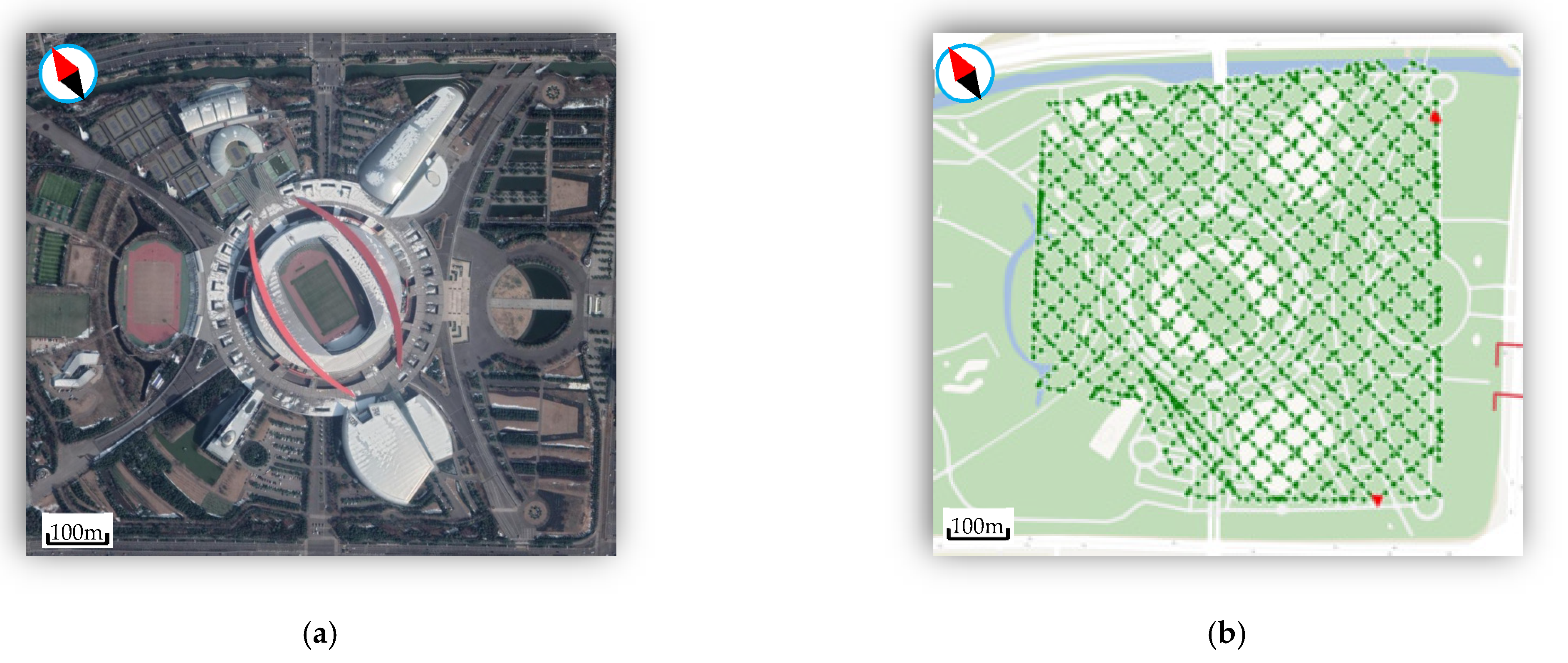
The test site is an Olympic sports center located in Nanjing, Jiangsu, China. It covers an area of about 0.9 km². As shown in Figure 4a, there are large stadiums, staggered roads, and rich landscapes, all of which are typical urban elements involved in drone photogrammetry missions.

The drone device used is a DJI4-RTK (SZ DJI Technology Co., Ltd, Shenzhen, China), which integrates sensors such as a GNSS receiver, an inertial navigation system, and a digital camera. The flying height of the drone is set to 100 m. From this height, the ground resolution of pixels is about 2.74 cm. The vertical and horizontal overlaps are set to 80% and 75%, respectively, to ensure good image overlaps. After three sorties of flights, 1455 images with a resolution of 4864 × 3648 pixels were recorded in total. The shooting positions of each images are shown in Figure 4b.

In practice, non-standardized GCPs are often established on road traffic signs (RTSs), whose corners are preferred. Therefore, RTSs are selected as the verification objects in this paper, acting as the aforementioned non-standardized GCPs. As shown in Figure 5 five different RTS instances are selected, carrying the non-standardized GCPs denoted as GCP1~GCP5. The shape types of the selected RTSs include hollow rectangles, solid rectangles, hollow diamonds, grid rectangles, and solid arrows, covering the commonly seen types.

3.2. Efficiency of the ROIs Extraction

For each of GCP1~GCP5, two images with distinct shooting angle differences are selected as the root images, and the remaining images are taken as leaf images. The imagery pixels of the GCPs in the root images are manually positioned. Then, the SIFT algorithm performs feature detection on the root images, and the feature correspondences are built with brute-force matching. Based on the 2d–2d feature correspondences from the root images, the poses of the root images are recovered with the epipolar constraint. Next, the feature correspondences from the root images are triangulated to reconstruct the 3d point cloud. After that, feature detection is also performed on the leaf images with the SIFT algorithm. Brute-force matching is then executed between the features from the leaf images and 3d points. Based on the 3d–2d feature correspondences from the leaf images and the 3d structure, the poses of the leaf images are recovered with the perspective constraint. Finally, we search ROIs along with the projection rays when the previous steps are completed. Among the total 1455 drone images, 93, 91, 85, 90, and 61 ROIs containing target GCPs were found for GCP1~GCP5, respectively. These ROIs are all squares of 30 pixels wide.

Table 1. Time cost for extracting ROIs in the case study.

Step 1	Duration	Proportion
Feature detection (SIFT)	14 min	24.1
Feature matching (brute)	33 min	56.9
Image pose recovery	10 min	17.2
ROI search and extraction	1 min	1.8

¹ SIFT feature detection is executed by a GPU (GTX1050Ti); Other steps are executed by a CPU (AMD 3900X).

shows the time taken by the computer to complete this part of the work. The total time is 58 min, where feature detection and feature matching account for 24.1% and 56.9%, respectively. The duration of this operation is not short, but it is still efficient compared with manual operation. Assuming that it takes 2 s to process an image manually, it sums to 1242.5 min for positioning GCP1~GCP5 in 1455 images. If the time for checking and correcting is also included, the manual method will take longer. Therefore, using the method proposed in this paper can significantly improve the efficiency of positioning GCP pixels. Compared with manual operation, it can save at least 95% of the time cost.

3.3. Performance of the ROIs Screening

There are differences in the quality level of the ROIs, some of which are low-quality due to negative factors. As shown in Figure 6, according to the clarity and completeness of the road traffic signs in the area of interest, these ROIs can be roughly divided into three categories: the high-quality, the marginal, and the disturbed. The ROIs of the first category are clear and complete, accounting for the main proportion. The second category is a set of ROIs whose locations are close to image boundaries. Furthermore, the rest of ROIs can be grouped as the third category, the disturbed. There are trees, vehicles, and other obstructions in the disturbed ROIs, making it hard to recognize RTSs.

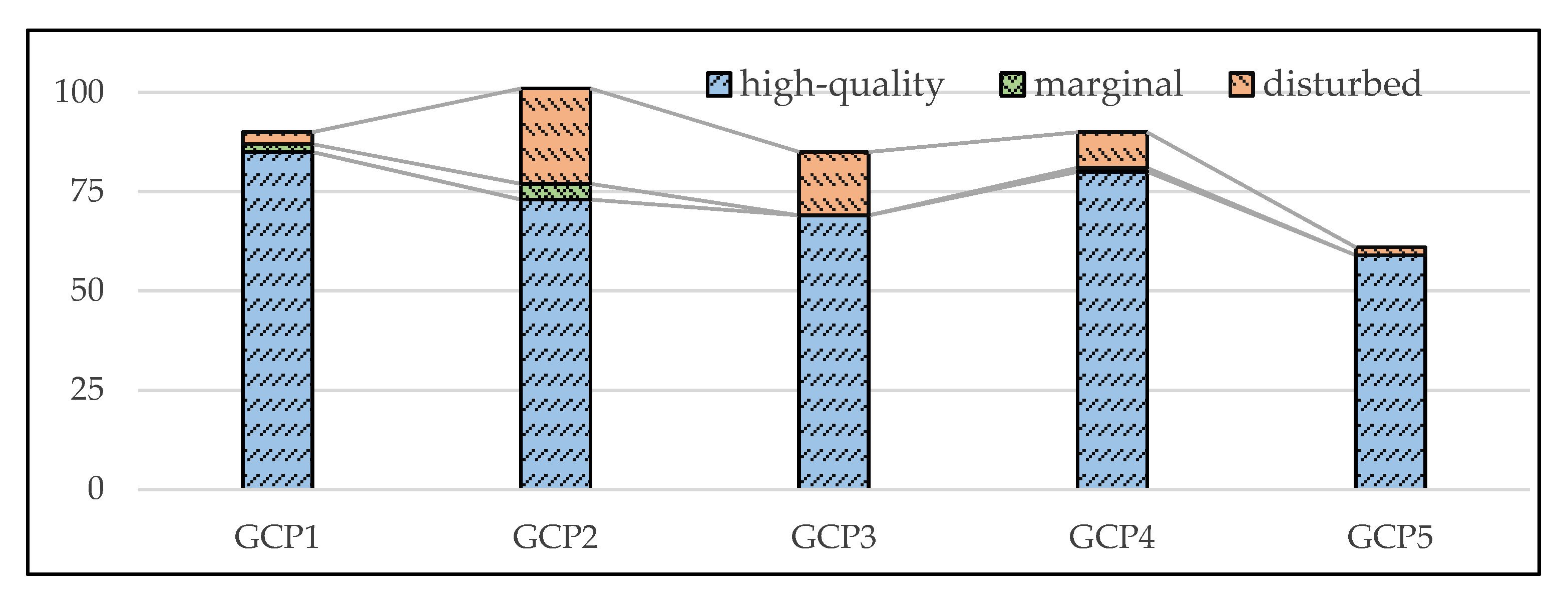
The histogram of these three categories for GCP1~GCP5 is shown in Figure 7. It can be found that there is a distinct difference in the high-quality proportions between the five GCPs. For example, the proportion of the high-quality ROIs corresponding to GCP1 reached 94.6%, while the proportion corresponding to GCP2 was only 69.2%. The low proportions of high-quality corresponding to GCP2, GCP3, and GCP4 may be because the roads where these GCPs locate are narrow, and they are more susceptible to be disturbed by things like trees and buildings. Moreover, some ROIs are extracted from the marginal zone of the drone images, and the neighborhood pixels are not complete, whose proportion is low, about 1.9%.

Low-quality ROIs tend to cause unexpected results when positioning GCP pixels, so they need to be identified and filtered before carrying out the positioning of GCP pixels. First, the Canny algorithm [34] is used to obtain the edge feature of the ROIs. Then, the one-dimensional entropy and the two-dimensional entropy are calculated based on the edge distribution. The statistical characteristics of the entropy values are listed in

Table 2. The statistical result of the entropy values of the edge distribution for five GCPs.

Entropy Item	GCP Label	Total Counts	Mean	Standard Deviation	1st Quantile	2nd Quantile	3rd Quantile
1-d entropy	GCP1	93	0.135	0.032	0.120	0.130	0.142
	GCP2	91	0.172	0.051	0.139	0.153	0.198
	GCP3	85	0.130	0.068	0.090	0.104	0.127
	GCP4	90	0.168	0.054	0.129	0.141	0.207
	GCP5	61	0.052	0.019	0.041	0.050	0.063
2-d entropy	GCP1	93	0.464	0.090	0.416	0.447	0.490
	GCP2	91	0.639	0.165	0.537	0.598	0.680
	GCP3	85	0.454	0.216	0.330	0.365	0.434
	GCP4	90	0.595	0.179	0.458	0.510	0.727
	GCP5	61	0.185	0.067	0.145	0.185	0.214

.

A violin chart for the distribution of entropy values is shown in Figure 8, composed of five subfigures for GCP1~GCP5. The left column in each subfigure represents 1-d entropy, while the right column represents 2-d entropy. It is found that the probability density curves of 1-d entropy and 2-d entropy are both spindle-shaped, which reflects that the entropy values are of solid clustering. In other words, an entropy value is closer to the mean value, the greater density is. It is also worth noting that the probability density curves in Figure 8b–d have secondary peaks far away from the main peaks. This may be due to a significant amount of low-quality ROIs for GCP2, GCP3, and GCP4. It reflects that the entropy values of the low-quality ROIs are significantly different from those of the normal ROIs, which further indicates that it is reliable to use entropy to characterize the quality of ROIs.

After obtaining the entropy quantiles of ROIs, the entropy anomaly recognition fences are computed for GCP1~GCP5, respectively. The ROIs whose entropy values fall within the fences are judged as normal, and the others are considered as outliers. The results are listed in

Table 3. The classification result by the adjusted boxplot for the five GCPs.

GCP Label	Total Counts	Fences for 1-d Entropy		Fences for 2-d Entropy		Within Fences (Normal)	Beyond Fences (Outlier)
		Lower	Upper	Lower	Upper
GCP1	93	0.064	0.226	0.185	0.658	90	3
GCP2	91	0.073	0.283	0.198	0.745	66	25
GCP3	85	0.057	0.198	0.213	0.789	70	15
GCP4	90	0.085	0.330	0.242	0.894	75	15
GCP5	61	0.023	0.085	0.089	0.328	58	3

. For example, 3, 25, 15, 15, and 3 were judged to be abnormal among 93, 91, 85, 90, and 61 ROIs for GCP1~GCP5. Figure 9 shows several samples of the edge features of normal and low-quality ROIs.

The result of fences-based low-quality ROI identification is not entirely accurate, and there may be some cases of wrong judging. Therefore, to evaluate actual accuracy, the results from the adjusted boxplot were compared with the manual classification results in Figure 6. Furthermore, the sensitivity and specificity are calculated as follows:

$$\begin{gathered} \mathrm{sensitivity}=\frac{\mathrm{TP}}{\mathrm{TP}+\mathrm{FN}} \\ \mathrm{specificity}=\frac{\mathrm{TN}}{\mathrm{TN}+\mathrm{FP}} \end{gathered}$$

(11)

where TP, FP, TN and FN denote the counts of true positives, false positives, true negatives, and false negatives, respectively. The results are shown in

Table 4. The accuracy evaluation of the adjusted boxplot.

GCP Label	Total Counts	Correctness				Sensitivity	Specificity
		TP	FP	TN	FN
GCP1	93	3	0	0	90	100.0%	100.0%
GCP2	91	24	1	1	66	96.0%	98.5%
GCP3	85	15	0	2	68	88.2%	100.0%
GCP4	90	13	2	0	75	100.0%	97.4%
GCP5	61	0	3	0	58	100.0%	95.1%

. As Table 4 shows, the average sensitivity is 96.84%, and the average specificity is 98.2%, both of which are at high levels. Therefore, the adjusted boxplot is valid for low-quality ROI recognition and has high accuracy.

3.4. Accuracy of the GCP Pixels Positioning

After screening ROIs, low-quality ROIs were filtered out as much as possible. There remai 90, 66, 70, 75, and 58 high-quality ROIs for GCP1~GCP5, respectively. First, the FAST-12 corner detector is used to detect the corners in the high-quality ROIs, and a set of candidate pixels that may be GCP pixels are obtained. Then, distances between the candidate pixels and the ROI centers are calculated, and the pixel with the smallest distance is selected as the pixel of interest. After this, the sub-pixel optimization is carried out to pursue higher positioning precision with the Förstner algorithm. Figure 10 shows some of the positioning results, and it intuitively shows expected goals.

In order to evaluate the accuracy of the positioning results, a manual check is carried out. The results are listed in

Table 5. The accuracy evaluation of GCP pixels positioning results.

GCP Label	Total Counts	Correctness 1			Accuracy Rate 2
		Positive	Negative	Unclear
GCP1	93	90	0	0	100.0%
GCP2	91	63	2	1	95.5%
GCP3	85	68	0	2	97.1%
GCP4	90	71	4	0	94.7%
GCP5	61	57	1	1	98.7%

¹ Positive results are those proven to be correct after manual check; Negative results are those proven to be wrong after manual check; The rest are called unclear. ² The accuracy rates are calculated with $\mathrm{accuracy}=\frac{\mathrm{positive} \mathrm{counts} }{\mathrm{total} \mathrm{counts}}$.

, and the average accuracy is 97.2%. It is worth noting that the accuracy values for GCP2, GCP3, and GCP4 are slightly lower than those for GCP1 and GCP5. This may be because the ROIs of GCP2, GCP3, and GCP4 are more complex than GCP1 and GCP5. Nevertheless, as Table 5 shows, excellent positioning has been achieved through corner detection and sub-pixel optimization.

4. Discussion

As a widely studied topic in the photogrammetry field, automatic or semi-automatic methods for positioning GCPs in images have been studied for many years. In some literature, universal fiducial markers, such as CCTs and PCTs, were introduced to act as GCPs. The benefits of doing this are significant since the participation of fiducial markers dramatically reduces the difficulty of algorithm design based on regular image characteristics. This kind of treatment is of great value because it opens the way for automated processing GCPs and is still prevalent in drone photogrammetry software packages. However, the introduction of artificial markers limits flexibility. On the contrary, directly placing GCPs on natural objects is more flexible and requires less logistical input for maintaining GCPs, so that is why developing the methods for fast positioning non-standardized GCPs in drone images is of strategic interest.

This paper proposed a method for fast positioning non-standardized GCPs in drone images. The research work has the following highlights. The first point is that stereo vision technologies are introduced during the acquisition of ROIs to avoid the potential risk from wrong ROIs effectively. The second point is that an adjustment is made to the traditional Tukey’s fences to improve the flexibility and accuracy of recognizing abnormal ROIs. The third point is that the corner feature is used as the detection target for searching the pixels of interest. Moreover, sub-pixel optimization is included for pursuing precise coordinates of the GCP pixels.

Efficiency and accuracy are vital evaluation aspects for an automated method, so quantitative results are provided in the experimental implementation to show the performance of the proposed method. As an alternative to manual operation, selecting manual operation as a primary benchmark is feasible to illustrate efficiency improvement. It shows that the proposed method can save at least 95.0% of the time consumption compared with manual operation, and the average accuracy reached 97.2%. We further tried to include data from other literature as secondary benchmarks. However, unfortunately, little was found, and this trouble hindered the comparison of efficiency and accuracy with other works. Nevertheless, we can infer the performance of their works by analyzing their technical frameworks. For example, the works of Deng et al. [19] and Sina et al. [21,22] did not consider the step of searching and screening ROIs, but instead, they handed it over to specific image feature detectors, which go straight to get the pixels without secondary check steps. Similarly, Purevdorj et al. [17] and Cao et al. [23] turned to template matching and did not include secondary check steps either. Their works are fast in processing speed, almost real-time. However, due to the lack of specific steps to avoid wrong detections, their methods are theoretically more prone to errors. In contrast, our paper emphasizes the error-proofing mechanism during method framework design to achieve high accuracy, although processing is slightly slower. It is worth noting that the method proposed in this paper depends lowly on the form of GCPs, especially during searching and screening the ROIs. Only in the section of pixel positioning, a specific strategy is adopted, i.e., corner detection. If practicers want to apply this method to other forms of non-standardized GCPs, they just need to modify the pixel positioning strategy according to the target characteristics. For example, centroid features are efficient and effective for GCPs located at the centers of uni-color blocks. In short, the method proposed in this paper is of solid flexibility.

Although the proposed method has achieved satisfactory results in case verification, some points are still worthy of further study. On the one hand, some technical aspects of the method are currently single-track designed and may need consideration on a multi-track framework for further development. On the other hand, due to the engagement of some time-consuming steps, such as image feature detection and feature matching, the efficiency of the proposed method needs to be further improved.

5. Conclusions

This paper proposed a method for fast positioning non-standardized GCPs in drone images. The research work is concentrated on three aspects: the search of ROIs, the filtering of abnormal ROIs, and the positioning of GCP pixels. Firstly, the relative spatial poses of drone images are recovered with multi-view constraints from feature correspondences, and image regions of interest are extracted through ray projection. Secondly, visibility check and outlier removal are carried out with an adjusted boxplot of edge-based image entropy. Finally, the GCP pixels are positioned through corner detection and sub-pixel optimization. A case study was carried out to evaluate the performance of the proposed method, and the results show that the time used by this method can save at least 95% of the time cost compared with manual operation. In addition, the average sensitivity of filtering ROIs reached 96.84%, and the average positioning accuracy of GCPs reached 97.2%. Therefore, the method proposed in this paper is of enlightening value.