Abstract
This paper reports the results of field measurements of wave breaking modulations by dominant surface waves, taken from the Black Sea research platform at wind speeds ranging from 10 to 20 m/s. Wave breaking events were detected by video recordings of the sea surface synchronized and collocated with the wave gauge measurements. As observed, the main contribution to the fraction of the sea surface covered by whitecaps comes from the breaking of short gravity waves, with phase velocities exceeding 1.25 m/s. Averaging of the wave breaking over the same phases of the dominant long surface waves (LWs, with wavelengths in the range from 32 to 69 m) revealed strong modulation of whitecaps. Wave breaking occurs mainly on the crests of LWs and disappears in their troughs. Data analysis in terms of the modulation transfer function (MTF) shows that the magnitude of the MTF is about 20, it is weakly wind-dependent, and the maximum of whitecapping is windward-shifted from the LW-crest by 15 deg. A simple model of whitecaps modulations by the long waves is suggested. This model is in quantitative agreement with the measurements and correctly reproduces the modulations’ magnitude, phase, and non-sinusoidal shape.
1. Introduction
Wave breaking plays a crucial role in various air–sea interactions and remote sensing areas and thus has been the subject of intensive research over the past few decades (see, e.g., [1,2,3,4,5]). Wave breaking of wind-driven waves contributes substantially to air-sea gas exchange [6,7,8], wave energy and momentum dissipation [9,10,11], and generation of turbulence in the ocean near-surface layer [12,13,14]. Wind-wave modeling and forecasting need spectral parameterization for wave breaking [15,16]. Wave breaking affects radar backscattering [17,18,19,20] and microwave emission [21,22] of the sea. Wave breaking is also very sensitive to the energy disturbances caused by wave interactions, with sub- and mesoscale surface current gradients being an important component of the wave energy balance. As a consequence, various ocean phenomena, such as internal waves, eddies, current fronts, shallow water bathymetry are displayed on the ocean surface in the form of spatial anomalies of wave breaking parameters tracing the surface current features [23,24,25,26,27]. This opens a promising opportunity for monitoring the ocean dynamics using passive and active microwave satellite remote sensing [28,29,30]. Due to whitecapping, video processing is a traditional approach for the in-situ investigation of wave breaking statistics and space-time characteristics of “individual” breaking events (see, e.g., [31,32,33,34]).
Long surface waves modulate the breaking of short wind waves [35,36,37], resulting in enhancement of wave breaking around the crests and damping in the long wave throughs. This effect, observed in both the laboratory and the field, has important applications. Modulations of wave breaking lead to variations of radar returns along the wavelength of long waves. This, on the one hand, significantly contributes to the radar modulation transfer function, which is necessary to retrieve wave parameters from the radar signal [19]. On the other hand, modulations of radar backscattering by long surface waves provide a significant, if not dominant, contribution to the mean Doppler shift of radar backscatter from the ocean surface. Errors of the quantitative estimates of such radar modulations predetermine the accuracy of the ocean surface current retrieval from the Doppler shift anomalies [38,39,40]. In the context of the air–sea interaction, the effect of wave breaking [35,37] and short-wave spectrum [41] modulations on the aerodynamic roughness along the dominant surface waves profile, significantly amplify (by factor two to three) momentum and energy transfer from the wind to waves [42]. Hence, a better understanding of the wave breaking modulations mechanism can directly contribute to a better understanding of the momentum and energy exchange between atmosphere and ocean on regional and global scales.
Modulations of a certain characteristic of the sea surface, for example, whitecaps coverage, , by long/dominant surface waves, can be described in terms of the modulation transfer function (MTF), which assumes that varies above the long-wave as:
where is the MTF magnitude, means mean value of , is the steepness of modulating wave with elevations , is the wave amplitude, is the phase, is the long-wave wavenumber, is the phase shift between and , a positive value of means a lag of modulations relative to (shift of the modulations towards the backward long-wave slope). MTF is the common terminology for describing interactions of short and long surface waves [43,44,45], radar scattering [19,46], and wave breaking modulations by long surface waves [35,37]. Experimental estimates of whitecaps MTF remain very scarce, and to our knowledge, they are limited by the results reported in [35,37]. According to these data, the magnitudes of the whitecaps MTF are surprisingly large, about 20. This means that wave breaking variations scaled by the mean value are 20 times larger than the steepness of modulating waves, pointing to the nonlinear nature of breaking modulations. Since experimental estimates of wave breaking modulations are extremely limited, new measurements are in great demand to get a deeper insight into the physics of this phenomenon.
In this paper, we report field investigations of the whitecaps modulations by long surface waves performed from a Black Sea research platform, using video recordings of the sea surface. A description of the field experiment, data, and method of data processing is presented in Section 2. Results and interpretation of the data in terms of the MTF revealing large modulations are presented in Section 3. In Section 4, we suggest a simple model of whitecaps modulations that describe quantitatively empirical results. Discussion and conclusion are given in Section 5 and Section 6.
2. Field Experiment
2.1. General Description
The experimental studies were carried out in October 2018 from a Black Sea research platform near the village of Katsiveli. The platform is located about 0.5 km offshore in about 30 m deep water. A more detailed description of the platform and types of wind-wave conditions at this site were reported in [47]. This study was performed under conditions of developing wind waves coming from the open sea without swell.
The wave breaking events were recorded using a digital video camera with a recording rate of 50 frames per second and a resolution of 1920 × 1080 pixels. The camera was mounted at the height of 12 m and directed at 35–40° to the horizontal, which provides a resolution of 2 cm at the water surface. The camera looked opposite to the general direction of dominant waves, which always coincided with the wind direction. Eight video records of length from 60 to 90 min collected at steady wind conditions are used in this study.
Elevations of the sea surface were recorded by a wire wave gauge located in the field of view of the video camera (see Figure 1) at the end of an 11 m long boom to minimize the platform disturbances. The wind speed and direction at a height of 23 m, air temperature and humidity at a height of 19 m, and temperature in the upper meter of water were measured continuously from the platform using Davis 6152EU meteorological station.

Figure 1.
Video frame with wave gauge boom and rectangle (in green) of the sea surface for studying the wave breaking modulations. A green point in the rectangle shows the interception of the wave gauge wire with the sea surface. The insets show (top) an enlarged fragment of the frame and (bottom) a period of the sea surface elevation recording, where an arrow marks the instant of time corresponding to this frame.
Frequency spectra of sea surface elevations, , spectral peak frequencies, , and significant wave heights, ( is the elevation variance), were calculated conventionally [48]. The wind speed at 10 m, , was calculated according to the algorithm of Fairall et al. [49]. Mean (over records) values of the wind speed, the spectral peak frequencies, the significant wave heights, the measure of wave ages, ( is the phase velocity of the spectral peak waves), air and water temperatures for all the records are listed in Table 1.

Table 1.
Measurement summary.
2.2. Data
Video recordings were processed using the algorithm suggested by Mironov and Dulov [32]. The pixel coordinates in video frames were transferred into horizontal coordinates at a zero-height plane, using known observation geometry. Only the active breakings belonging to “phase A” of Monahan and Wolf [50] were extracted from image sequences. The spots of residual foam left by whitecaps were automatically filtered out based on the distinction of their advancing velocity from the whitecaps one (see [32] for details). Areas of all active breaking at each time instant and their mean velocities were obtained to form the resulting datasets for each of the video recordings. Table 1 shows the whitecap coverage percentage, , calculated from the data.
Figure 2 shows spectral distributions of whitecap coverage over frequencies, (), together with wave spectra. The gives the contributions to whitecap coverage from frequency interval . It differs from Phillips’ breaking crest distribution reported in experimental studies (see, e.g., [32,33,34,51]). As suggested by Phillips [2], the velocity of a breaking front is equal to the phase velocity of the breaking wave generating the whitecap. Therefore, we obtained the by converting the measured whitecap velocities to frequency as , using deep water dispersion relation for gravity waves, where is the acceleration of gravity. On the other hand, if we suggest, following [9,52], that whitecaps move slower than the phase velocity, e.g., , the spectrum of whitecaps coverage is to be modified, as shown in Figure 2.
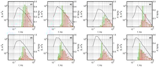
Figure 2.
Frequency spectra, , (solid line) and distributions of whitecap coverage over frequency, , for (red bars) and for (green bars) for all experimental runs.
As follows from Figure 2, only waves from the spectral interval approximately above double spectral peak frequency are breaking. Correspondingly, the length of modulating dominant waves exceeds the length of breaking waves by a factor of three to four. Thus, these data are suitable for analyzing the modulation of wave breaking from the equilibrium range by long waves of spectral peak.
2.3. Processing Procedure
The main goal is to compare simultaneously measured whitecap coverage and long-wave elevations that require special synchronization of the video camera and wave gauge data records. To that end, time-series of wave gauge and sound output of the video camera were recorded into a united file. The cross-correlation technique (see, e.g., [53]) was used for syncing the same time series from wave and video-sound recordings in the data processing. The accuracy of synchronization is 1 millisecond.
Only wave breaking events falling into the rectangular box on the sea surface (see Figure 1) were taken into account for comparison with the wave-gauge signal. The rectangle of m2 size was extended along the crests of long waves and centered at the wave-gauge position. Modulations of sea surface brightness visualize the long-wave in video recording (see, e.g., [54]). The coherence of sea brightness and the wave-gauge signal in any point of the rectangle was not less than 0.7, which allows linking whitecaps to the long-wave phase. An error in the determination of the phase can be estimated as:
where is wavelength and is the rectangle width across the long-wave crest, which for typical wave conditions gives .
Figure 3 shows the time series of wave elevations, , and instantaneous whitecap coverage of the rectangle, . Since breaking occurs very rarely, the realization of has the form of separate spikes against zero background, so the spectral technique for studying the radar MTF, described by Plant [50], is not applicable in this case. Therefore, we used the procedure of individual-wave analysis suggested by Dulov et al. [35]. After smoothing to filter out short waves, the elevation records were split into consecutive periods between zero up-crossings, . Augmenting them with corresponding periods of whitecap coverage series, , we obtained data subsets characterizing individual waves (for an example of an individual wave see Figure 3). For each of the individual waves, we introduced the wave period, , as the time-length of the subset, and the wavenumber:
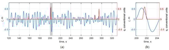
Figure 3.
An example of time-series (a) of wave elevation,
(blue), and whitecap coverage, , (red), and (b) zoomed individual wave period corresponding to the grey-marked part of the recording.
To compare different individual waves, we converted the time to the phase of the long-wave:
where is the instant of the first zero up-crossing, and considered the dimensionless elevation profiles:
Maximum values of represent the wave steepness for sinusoidal waves. As a result, several hundred individual-wave subsets were obtained from each of the experimental runs (see Table 1).
3. Results
Figure 4 shows averaged individual-wave profiles for each of the runs, and exhibiting phase-resolved whitecaps distribution. The whitecap coverage profiles were normalized with their mean values (see Table 1). Amplitudes of averaged dimensionless elevation profiles, , are also listed in Table 1. Hereinafter, confidence intervals correspond to a double standard error.
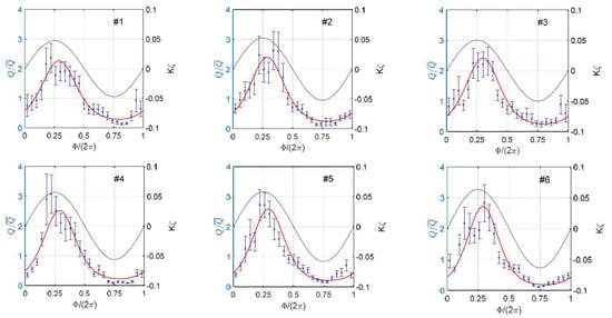
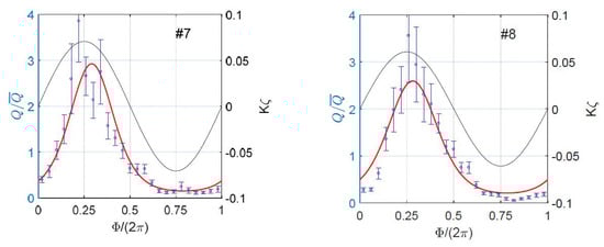
Figure 4.
Averaged profiles of normalized whitecap coverage (symbols with double-standard-error bars) and dimensionless wave elevations (black lines) along the wavelength of individual waves for all experimental runs. According to the definition of phase , the wave in Figure 4 runs from the right to the left. Red lines show model calculations for measured characteristics , , (see Table 1) and model parameters , .
In all the graphs, a strong enhancement of wave breaking takes place around the wave crests with a discernible shift to the backward (upwind) slope. Whitecap coverage profiles are clearly deviated from the sinusoidal shape, in contrast to wave elevation, showing a nonlinear connection between them. We describe the wave breaking modulations as:
where and means averaging over a period of the long wave. For small wave steepness, , Equation (2) reduces to Equation (1), which is a traditional linear description of modulations induced by long-waves in radar signals [46] or wave breaking [35,37], where is the modulation transfer function, and positive phase shift corresponds to shift of modulations maximum on the backward slope of the modulating wave.
Figure 5a,b, combining all the data, demonstrate better applicability of nonlinear description (2) for data fitting using a sinusoid. Moreover, nonlinear description (2) appears to be inherent in our data, as confirmed in Appendix A. Fitting the with , we obtain that an increase in leads to linear growth of remaining constant, see Figure 5c,d. Least-square estimates gives:
which are consistent with linear estimates and reported in [35]. It should be noted that the observed phase shift is also in concord with the measurements [36], where a maximum of small-scale breaking detected using IR imagery was found on the rear slope of the modulating waves.
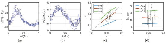
Figure 5.
To data analysis: collapsing all the data using (a) linear (2) and (b) nonlinear (1) representations; (c) amplitudes and (d) phase shifts in fitting the using according to (1) as a function of long-wave steepness for all recordings. Black dashed lines show least-square estimates (3). Colored solid lines show model calculations for mean data characteristics m/s and .
Figure 6 shows wind dependences of modulation parameters. The results of [35,37] obtained using linear representation (1) are also shown for comparison. Though wind dependences are weak, the same trends are evident for all the datasets. Some bias of estimations [37] is probably caused by residual foam, which was not completely removed in their study, and accounting for small-scale, microwave breaking.
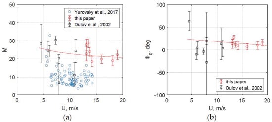
Figure 6.
Modulation parameters (a) and (b) as a function of wind velocity . Symbols show data, lines show model calculations for mean-over-data , and model parameters and .
4. Modelling
4.1. Governing Equations
Modulations of short wind wave spectrum by long-waves orbital velocities are modeled using the kinetic equation [55,56]:
where is the short-wave wavenumber vector, is frequency linked to wavenumber via the dispersion relations for deep water, ; is the wave action spectrum, related to the energy (elevation) spectrum as ; is a component of the group velocity of waves, is the horizontal component of the long-wave orbital velocity, and . Terms in the right-hand side of (4) describe the wind input, , nonlinear wave–wave interactions, , and dissipation due to wave breaking, .
Spectral sources on the right-hand side (4) are not exactly known. Following [2,18,57], we adopt the wind input in the form of:
where is the wind growth rate, is the friction velocity, and is the wind direction. Although the nonlinear energy transfer is important for the development of spectral peak waves [15], its role in the equilibrium range dynamics and its modulations is probably not important, and this term is further omitted. Following [2], the dissipation rate can be expressed through the length of wave breaking fronts, , as:
where is Duncan’s [1] empirical constant, is the breaker advancing velocity with varying in the range of [2,9,52]. The same quantity, , defines the fraction of the sea surface covered by whitecaps [2,18]:
where is the averaged ratio of the whitecap width to the length of wave generating the whitecap, and an integration domain in (7) corresponds to the range of breaking waves observed in an experiment. For the uniform conditions (when waves are stationary and there is no current), the balance between wind input (5) and dissipation (6) results in the following background relationship for :
where is the saturation spectrum, is its value in the absence of currents (background spectrum). Korinenko et al. [51] tested relationship (8) against the field measurements and found its validity. However, relation (8) is not valid in the presence of the current. On their nature, wave breaking characteristics, e.g., as well as the wave breaking dissipation, , are strongly nonlinear functions of the spectral level. Following [2,18,54,58], we parameterize spectral distribution of breaking fronts and wave breaking dissipation as power functions of the wave spectrum:
where is defined by (8). These expressions correspond to the Phillips’ theory of equilibrium range [2] if and to the Donelan and Pierson dissipation model [58] if . For the background conditions, when , relation (10) is reduced to (6) with (8). As it follows from (9) and (10), any deviations of the wave spectrum, , from the background one, , result in an amplified nonlinear response of wave breaking intensity (9) and the energy dissipation (10).
Equation (4) with wind input (5) and dissipation (10) close the model of short-wave spectrum modulation by long surface waves. Once spectrum modulations are found, corresponding modulations of whitecaps coverage could be found from (9) and (7). However, Equations (7) and (9) do not account for the finite lifetime of whitecaps, which is essential when it is comparable with the long-wave period. The reason is the following: whitecap moves with velocity , and during its life span , it lags from the long-wave profile moving with velocity . Since the details of whitecap time-evolution are not exactly known, we introduce this effect phenomenologically, defining along LW profile as:
where , , and are long-wave phase, wavenumber, and phase velocity, respectively, is the phase shift between whitecaps and dissipation, is the whitecap lifetime with as an empirical constant that does not depend on .
We consider the output of the model as:
which does not depend on empirical constants and as follows from model equations. Equations (4)–(11) completely formulate the model of long-wave manifestation in whitecapping. This model corresponds to the models of surface manifestation of the ocean current, suggested in [28,53], augmented with Equation (11) for whitecaps description, which takes into account the finite life span of the breaker.
4.2. Model Analysis
We performed model calculations specifying in (4) and in (8)–(10) for the case of as:
where , and is a constant on which the model output (10) does not depend as follows from an analysis of model equations. Such a form of wave spectrum reflects observed wide directional spread of waves at frequencies exceeding twice the spectral peak frequency (see, e.g., [59,60,61]). To specify the wind growth rate in (5), we calculated the friction velocity according to [49]. Details of model calculations are described in Appendix B. Calculation results very weakly depend on exact values of and . Therefore, further, we present them at and only.
According to model calculations, the MTF-value, , is mainly determined by parameter , while the phase shift, , is mainly determined by parameter . Their best matching to data results in:
as illustrated in Figure 5c,d. It is worthy to note that , found here as a value providing the best fit of whitecaps modulations to the data, corresponds to the exponent of the nonlinear dissipation originally suggested by Donelan and Pierson [58] from very different reasoning, to provide the best fit of short-wave spectrum to wind exponent of radar scattering from short gravity waves.
The model reproduces observed whitecap modulations (see Figure 4 and Figure 5) and their wind trend quite well (see Figure 6). Moreover, the model captures finer details of non-sinusoidal whitecap profiles, as demonstrated in Figure A1. These conclusions are related to the conditions of our experiments when the long waves and wind directions were aligned. However, the model simulations shown in Figure 7 suggest that similar features (high values of MTF, weak dependence on wind speed, and the shift of wave breaking to the rear face of the long waves) take place at any angle between the wind and swell. Additional experimental data are needed to confirm these predictions.
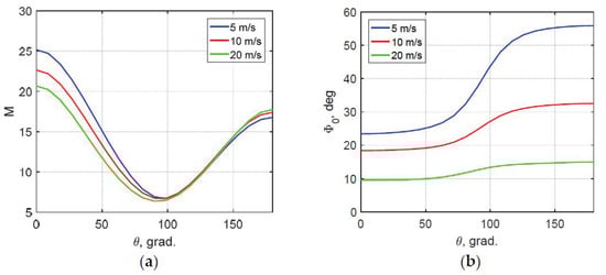
Figure 7.
(a) Magnitudes and (b) phase of the wave breaking MTF as a function of the angle between directions of the wind and long-wave, . Legends show wind velocities.
5. Discussion
Wave breaking intensity is a strongly nonlinear function of the wave saturation spectrum [2,9]. Therefore, small variations of short-wave spectrum, due to the interaction of waves with the surface current of an arbitrary origin, result in a significantly amplified response of wave breaking to the non-uniform surface currents (see, e.g., [24,25] for internal waves, and [26,28,29] for sub- and meso-scale ocean currents).
In general, as assumed, the effect of long-wave orbital velocities on the short-wave spectrum and wave breaking results from short–long waves interaction, the effect of bound harmonics, and the wind velocity undulations (see, e.g., [36,42,45]). The short–long waves interaction exhibits amplification of short waves on the long-wave crest and their suppression in the long-wave trough at any directions between the wind and the long waves. This fundamental mechanism was studied theoretically [62,63], numerically [64], and experimentally in both the field [43,44] and in the laboratory [45]. Physically, the modulation of short waves caused by short-wave straining and work of the radiation stress against orbital velocities of the long-wave [62]. In spectral representation, this effect in the present study is described by Equation (4).
Wave breaking, namely whitecaps coverage, is a strongly nonlinear function of the wave saturation spectrum. We modeled this effect phenomenologically, introducing a nonlinear link of breaking front lengths with spectral saturation level (9). This nonlinear relationship inevitably leads to a strong response of whitecaps to small wave spectrum modulations, providing high values of the wave breaking MTF . The wave breaking exponent in (9) is the main parameter defining the value of (see Figure 5c where slopes of calculated curves are equal to ). As whitecaps have a finite lifetime, they lag behind the long-wave crest, providing observed phase shift .
This study shows that neither effects of bound harmonics nor air–sea interaction is needed to understand wave breaking modulation by long waves. The short–long waves interaction and nonlinear transfer of short-wave steepness to wave breaking intensity provide a general explanation of wave breaking modulation by long waves, including high values of their modulation transfer function.
6. Conclusions
This paper reports results of investigations of modulations of wind-wave breaking by long surface waves using the data taken from the oceanographic platform in the Black Sea and modelling. The data are collected at moderate to high wind conditions, is in the range from 10 to 20 m/s, and thus supplement the few field measurements of wave breaking modulation reported before [35,37] for lower wind speeds, m/s.
As found, the distribution of whitecaps along the long-wave has a strong nonlinear shape with prevailing whitecapping on the crest of modulating wave and with almost full wave breaking suppression in the trough areas. We proposed a nonlinear representation of the whitecaps modulations in form (2), with a modulation transfer function of about 20. A simple model of whitecaps modulations by long surface waves is suggested, which reproduces the observations on the quantitative level. We modeled the strongly nonlinear response of wave breaking modulations to long waves introducing the wave breaking exponent (see Equations (9) and (10)). As found, the best fit of modeled whitecaps modulations to the data results in . It should be noted that Donelan and Pierson [58] found the same value for n from another reasoning, in the best fitting of the modeled wave spectrum to wind exponent of radar scattering from short gravity waves.
We anticipate that reported results on wave breaking modulations by long surface waves can be further used in different research applications, in particular for the investigation of radar Doppler scattering from the ocean surface, where hydrodynamic modulations of the radar facets by large-scale surface waves significantly contribute to the formation of the Doppler centroid anomaly [39,40].
Author Contributions
Conceptualization, V.N.K. and V.A.D.; methodology, V.A.D., V.V.M. and V.N.K.; software, A.E.K. and V.A.D.; formal analysis, V.V.M.; investigation, A.E.K.; data curation, V.V.M.; writing—original draft preparation, V.A.D. and A.E.K.; writing—review and editing, V.N.K. All authors have read and agreed to the published version of the manuscript.
Funding
This work was funded by the Russian Science Foundation Grant No. 21-17-00236.
Data Availability Statement
Data is contained within Figures of the article.
Acknowledgments
This work was funded by the Russian Science Foundation Grant No. 21-17-00236. Field measurements were performed as a part of the government assignment No. 0555-2021-000421-0004 at Marine Hydrophysical Institute of Russian Academy of Sciences.
Conflicts of Interest
The authors declare no conflict of interest.
Appendix A. On Analysis of the Nonlinear Shape of Whitecap Coverage Profiles
For quantifying the nonlinear connection between profiles of whitecap coverage modulations and longwave elevations, we used truncated Fourier expansion
and described modulations through four parameters:
where and distinguish the nonlinearity. Figure A1a–c shows the dependence of normalized amplitudes and phase shifts of the harmonics on the wave steepness . An increase in leads to linear growth of and quadratic growth of remaining the phase shifts constant. Least-square-estimates are:
For small wave steepness, Equation (2) reads:
that equivalent to (A1) if:
As follows from estimates (A2), Equations (A4) and (A5) are fulfilled in the limits of confidential intervals (, ). Figure A2d shows the correspondence of data to Equation (A3), where the dashed line is drawn for . Thus, our data support the representation (2) up to the order of .
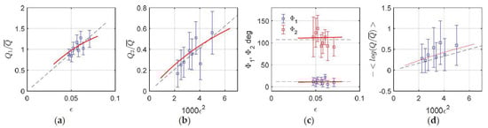
Figure A1.
Normalized amplitudes (a,b) and phase shifts (c) of the first two harmonics in (A1) as a Figure A2a–c and curve (d). Red lines show model calculations for mean data characteristics m/s and .
Figure A1.
Normalized amplitudes (a,b) and phase shifts (c) of the first two harmonics in (A1) as a Figure A2a–c and curve (d). Red lines show model calculations for mean data characteristics m/s and .

Appendix B. Calculation Procedure
If the field of currents (13) switches at , then model calculations reduce to solving an initial value problem to equations (4) with initial condition (12) for . The steady-state solutions of the problem at a big enough time model the whitecap response to periodical currents. In Section 4.2, we discussed model results based on this solution.
We considered on the grid log-spaced in and uniform in , where . rad/m that corresponds to the shortest waves, where breaking is resolvable in our experiments. For current velocity (11), after the transition to the frame moving with the long-wave phase speed through changing variables to , the Equation (4) reads:
where , and . Numerically, evaluating the term at every grid node, we considered (A6) as an ordinary differential equation and integrated it with initial conditions at , using a second-order Runge-Kutta scheme.
Figure A2a shows the process of converging to a steady-state solution for the integral measure, fractional whitecap coverage normalized with its initial value . After switching on the currents, whitecap production occurs more extensively on long-wave crests than on their troughs due to the nonlinearity of the wave dissipation. It leads to abrupt growth of the mean-over-period value of , , which is also shown in Figure A2a. Further whitecap coverage adjusts to periodical disturbances, and decreases to be slightly lower than its initial value. In this paper, the variable is used both in experiment and model analysis. Though the adjustment process lasts tens of long-wave periods, remains practically unchanged after the tenth period, see Figure A2b.
Figure A2.
Adjustment to periodical currents (11) for (a) whitecap coverage and its mean-over-period value and (b) their ratio showed for 40th and 15th periods. Calculations were performed for mean data characteristics , m/s, and model parameters and .
Figure A2.
Adjustment to periodical currents (11) for (a) whitecap coverage and its mean-over-period value and (b) their ratio showed for 40th and 15th periods. Calculations were performed for mean data characteristics , m/s, and model parameters and .
References
- Duncan, J.H. An Experimental Investigation of Breaking Waves Produced by a Towed Hydrofoil. Proc. R. Soc. Lond. A 1981, 377, 331–348. [Google Scholar] [CrossRef]
- Phillips, O.M. Spectral and statistical properties of the equilibrium range in wind-generated gravity waves. J. Fluid Mech. 1985, 156, 505–531. [Google Scholar] [CrossRef]
- Caulliez, G. Wind wave breaking from micro to macroscale. In Gas Transfer at Water Surface; Kyoto University Press: Kyoto, Japan, 2011; pp. 151–163. [Google Scholar]
- Babanin, A. Breaking of ocean surface waves. Acta Phys. Slov. 2009, 59, 305–535. [Google Scholar] [CrossRef]
- Melville, W.K. Wind-Wave Breaking. Procedia IUTAM 2018, 26, 30–42. [Google Scholar] [CrossRef]
- Thorpe, S.A. Bubble clouds and the dynamics of the upper ocean. Q. J. R. Meteorol. Soc. 1992, 118, 1–22. [Google Scholar] [CrossRef]
- Zappa, C.J.; McGillis, W.R.; Raymond, P.A.; Edson, J.B.; Hintsa, E.J.; Zemmelink, H.J.; Dacey, J.W.H.; Ho, D.T. Environmental turbulent mixing control sonair-water gas exchange in marine and aquatic systems. J. Geophys. Res. Lett. 2007, 34, L10601:1–L10601:6. [Google Scholar] [CrossRef] [Green Version]
- Andreas, E.L.; Mahrt, L.; Vickers, D. An improved bulk air–sea surface flux algorithm, including spray-mediated transfer. Q. J. R. Meteorol. Soc. 2015, 141, 642–654. [Google Scholar] [CrossRef]
- Rapp, R.J.; Melville, W.K. Laboratory measurements of deep-water breaking waves. Philos. Trans. R. Soc. London. Ser. A Math. Phys. Sci. 1990, 331, 735–800. [Google Scholar] [CrossRef] [Green Version]
- Thorpe, S.A. Energy loss by breaking waves. J. Phys. Oceanogr. 1993, 23, 2498–2502. [Google Scholar] [CrossRef]
- Hwang, P.A.; Sletten, M.A. Energy dissipation of wind-generated waves and whitecap coverage. J. Geophys. Res. 2008, 113, C02012:1–C02012:12. [Google Scholar] [CrossRef]
- Kudryavtsev, V.; Shrira, V.; Dulov, V.; Malinovsky, V. On the vertical structure of wind-driven sea currents. J. Phys. Oceanogr. 2008, 38, 2121–2144. [Google Scholar] [CrossRef]
- Rascle, N.; Chapron, B.; Ardhuin, F.; Soloviev, A. A note on the direct injection of turbulence by breaking waves. Ocean Model. 2013, 70, 145–151. [Google Scholar] [CrossRef] [Green Version]
- Schwendeman, M.; Thomson, J. Observations of whitecap coverage and the relation to wind stress, wave slope, and turbulent dissipation. J. Geophys. Res. (Oceans) 2015, 120, 8346–8363. [Google Scholar] [CrossRef]
- Janssen, P.A.E.M.; Hasselmann, K.; Hasselmann, S.; Komen, G.J. Parameterization of source terms and the energy balance in a growing wind sea. In Dynamics and Modelling of Ocean Waves; Komen, G.J., Cavaleri, L., Donelan, M.A., Hasselmann, K., Hasselmann, S., Janssen, P.A.E.M., Eds.; Cambridge University Press: Cambridge, UK, 1994; pp. 215–232. ISBN 0-521-47047-1. [Google Scholar]
- Filipot, J.-F.; Ardhuin, F. A unified spectral parameterization for wave breaking: From the deep ocean to the surf zone. J. Geophys. Res. 2012, 117, C00J08:1–C00J08:19. [Google Scholar] [CrossRef] [Green Version]
- Phillips, O.M. Radar returns from the sea surface—Bragg scattering and breaking waves. J. Phys. Oceanogr. 1988, 18, 1065–1074. [Google Scholar] [CrossRef]
- Kudryavtsev, V.; Hauser, D.; Caudal, G.; Chapron, B. A semiempirical model of the normalized radar cross-section of the sea surface Background model. J. Geoph. Res. (Oceans) 2003, 108, FET 2-1–FET 2-24. [Google Scholar] [CrossRef] [Green Version]
- Kudryavtsev, V.; Hauser, D.; Caudal, G.; Chapron, B. A semiempirical model of the normalized radar cross section of the sea surface, Radar modulation transfer function. J. Geophys. Res. (Oceans) 2003, 108, FET 3-1–FET 3-16. [Google Scholar] [CrossRef]
- Kudryavtsev, V.N.; Fan, S.; Zhang, B.; Mouche, A.A.; Chapron, B. On Quad-Polarized SAR Measurements of the Ocean Surface. IEEE Trans. Geosci. Remote Sens. 2019, 57, 8362–8370. [Google Scholar] [CrossRef]
- Anguelova, M.D.; Webster, F. Whitecap coverage from satellite measurements: A first step toward modeling the variability of oceanic whitecaps. J. Geophys. Res. 2006, 111, C03017:1–C03017:23. [Google Scholar] [CrossRef] [Green Version]
- Bettenhausen, M.H.; Anguelova, M.D. Brightness Temperature Sensitivity to Whitecap Fraction at Millimeter Wavelengths. Remote Sens. 2019, 11, 2036. [Google Scholar] [CrossRef] [Green Version]
- Thorpe, S.A.; Belloul, M.B.; Hall, A.J. Internal waves and whitecaps. Nature 1987, 330, 740–742. [Google Scholar] [CrossRef]
- Dulov, V.A.; Klyushnikov, S.I.; Kudryavtsev, V.N. The effect of internal waves on the intensity of wind wave breaking. Field observation. Sov. J. Phys. Oceanogr. 1986, 6, 14–21. [Google Scholar]
- Dulov, V.A.; Kudryavtsev, V.N. Imagery of the inhomogeneities of currents on the ocean surface state. Sov. J. Phys. Oceanogr. 1990, 1, 325–336. [Google Scholar] [CrossRef]
- Dulov, V.A.; Kudryavtsev, V.N.; Sherbak, O.G.; Grodsky, S.A. Observations of Wind Wave Breaking in the Gulf Stream Frontal Zone. Glob. Atmos. Ocean. Syst. 1998, 6, 209–242. [Google Scholar]
- Kubryakov, A.A.; Kudryavtsev, V.N.; Stanichny, S.V. Application of Landsat imagery for the investigation of wave breaking. Remote Sens. Environ. 2021, 253, 112144:1–112144:18. [Google Scholar] [CrossRef]
- Kudryavtsev, V.; Akimov, D.; Johannessen, J.; Chapron, B. On radar imaging of current features: Model and comparison with observations. J. Geophys. Res. 2005, 110, C07016:1–C07016:27. [Google Scholar] [CrossRef] [Green Version]
- Kudryavtsev, V.; Kozlov, I.; Chapron, B.; Johannessen, J.A. Quad-polarization SAR features of ocean currents. J. Geophys. Res. Oceans 2014, 119, 6046–6065. [Google Scholar] [CrossRef] [Green Version]
- Fan, S.; Kudryavtsev, V.; Zhang, B.; Perrie, W.; Chapron, B.; Mouche, A. On C-Band Quad-Polarized Synthetic Aperture Radar Properties of Ocean Surface Currents. Remote Sens. 2019, 11, 2321. [Google Scholar] [CrossRef] [Green Version]
- Melville, W.K.; Matusov, P. Distribution of breaking waves at the ocean surface. Nature 2002, 417, 58–63. [Google Scholar] [CrossRef]
- Mironov, A.S.; Dulov, V.A. Detection of wave breaking using sea surface video records. Meas. Sci. Technol. 2008, 19, 015405. [Google Scholar] [CrossRef]
- Kleiss, J.M.; Melville, W.K. Observations of wave breaking kinematics in fetch-limited seas. J. Phys. Oceanogr. 2010, 40, 2575–2604. [Google Scholar] [CrossRef]
- Sutherland, P.; Melville, W.K. Field measurements and scaling of ocean surface wave-breaking statistics. J. Geophys. Res. Lett. 2013, 40, 3074–3079. [Google Scholar] [CrossRef]
- Dulov, V.A.; Kudryavtsev, V.N.; Bol’shakov, A.N. A field study of white caps coverage and its modulations by energy containing waves. In Gas Transfer at Water Surface, Geophys. Monogr; Donelan, M.A., Drennan, W.M., Saltzman, E.S., Wanninkhof, R., Eds.; AGU: Washington, DC, USA, 2002; pp. 187–192. [Google Scholar] [CrossRef]
- Branch, R.; Jessup, A.T. Infrared Signatures of Microbreaking Wave Modulation. IEEE Geosci. Remote Sens. Lett. 2007, 4, 372–376. [Google Scholar] [CrossRef]
- Yurovsky, Y.Y.; Kudryavtsev, V.N.; Chapron, B. Simultaneous radar and video observations of the sea surface in field condi-tions. In Proceedings of the Electromagnetics Research Symposium-Spring (PIERS), St Petersburg, Russia, 22–25 May 2017; pp. 2559–2565. [Google Scholar]
- Johannessen, J.; Chapron, B.; Collard, F.; Kudryavtsev, V.; Mouche, A.; Akimov, D.; Dagestad, K.-F. Direct ocean surface velocity measurements from space: Improved quantitative interpretation of Envisat ASAR observations. Geophys. Res. Lett. 2008, 35, L22608:1–L22608:6. [Google Scholar] [CrossRef] [Green Version]
- Yurovsky, Y.Y.; Kudryavtsev, V.N.; Chapron, B.; Grodsky, S.A. Modulation of Ka-band Doppler Radar Signals Backscattered from the Sea Surface. IEEE Trans. Geosci. Remote Sens. 2018, 56, 2931–2948. [Google Scholar] [CrossRef] [Green Version]
- Yurovsky, Y.Y.; Kudryavtsev, V.N.; Grodsky, S.A.; Chapron, B. Sea Surface Ka-Band Doppler Measurements: Analysis and Model Development. Remote Sens. 2019, 11, 839. [Google Scholar] [CrossRef]
- Vincent, C.L.; Thomson, J.; Graber, H.C.; Collins, C.O. Impact of swell on the wind-sea and resulting modulation of stress. Prog. Oceanogr. 2019, 178, 102164:1–102164:30. [Google Scholar] [CrossRef]
- Kudryavtsev, V.; Chapron, B. On growth rate of wind waves: Impact of short-scale breaking modulations. J. Phys. Oceanogr. 2016, 46, 349–360. [Google Scholar] [CrossRef]
- Hara, T.; Plant, W.J. Hydrodynamic modulation of short wind-wave spectra by long waves and its measurement using microwave backscatter. J. Geophys. Res. (Oceans) 1994, 99, 9767–9784. [Google Scholar] [CrossRef]
- Hara, T.; Hanson, K.A.; Bock, E.J.; Uz, B.M. Observation of hydrodynamic modulation of gravity-capillary waves by dominant gravity waves. J. Geophys. Res. 2003, 108, 3028:1–3028:19. [Google Scholar] [CrossRef]
- Donelan, M.A.; Haus, B.K.; Plant, W.J.; Troianowski, O. Modulation of short wind waves by long waves. J. Geophys. Res. 2010, 115, C10003:1–C10003:12. [Google Scholar] [CrossRef] [Green Version]
- Plant, W.J. The Modulation Transfer Function: Concept and Applications. In Radar Scattering from Modulated Wind Waves; Komen, G.J., Oost, W.A., Eds.; Springer: Dordrecht, The Netherlands, 1989; pp. 155–172. [Google Scholar]
- Dulov, V.; Kudryavtsev, V.; Skiba, E. On fetch- and duration-limited wind wave growth: Data and parametric model. Ocean Model. 2020, 153, 101676. [Google Scholar] [CrossRef]
- Earle, M. Nondirectional and Directional Wave Data Analysis Procedures; NDBC Technical Document 96-01. Available online: www.ndbc.noaa.gov/wavemeas.pdf (accessed on 3 July 2021).
- Fairall, C.W.; Bradley, E.F.; Hare, J.E.; Grachev, A.A.; Edson, J.B. Bulk parameterization of air–sea fluxes: Updates and veri-fication for the COARE algorithm. J. Clim. 2003, 16, 571–591. [Google Scholar] [CrossRef]
- Monahan, E.C.; Woolf, D.K. Comments on “Variations of whitecap coverage with wind stress and water temperature. J. Phys. Oceanogr. 1989, 19, 706–709. [Google Scholar] [CrossRef] [Green Version]
- Korinenko, A.E.; Malinovsky, V.V.; Kudryavtsev, V.N.; Dulov, V.A. Statistical Characteristics of Wave Breakings and their Relation with the Wind Waves’ Energy Dissipation Based on the Field Measurements. Phys. Oceanogr. 2020, 27, 472–488. [Google Scholar] [CrossRef]
- Banner, M.L.; Peirson, W.L. Wave breaking onset and strength for two-dimensional deep-water wave groups. J. Fluid Mech. 2007, 585, 93–115. [Google Scholar] [CrossRef] [Green Version]
- Vieira, M.; Guimarães, P.V.; Violante-Carvalho, N.; Benetazzo, A.; Bergamasco, F.; Pereira, H. A Low-Cost Stereo Video System for Measuring Directional Wind Waves. J. Mar. Sci. Eng. 2020, 8, 831. [Google Scholar] [CrossRef]
- Yurovskaya, M.V.; Dulov, V.A.; Chapron, B.; Kudryavtsev, V.N. Directional short wind wave spectra derived from the sea surface photography. J. Geophys. Res. (Oceans) 2013, 118, 4380–4394. [Google Scholar] [CrossRef]
- Phillips, O.M. On the response of short ocean wave components at a fixed wave number to ocean current variations. J. Phys. Oceanogr. 1984, 14, 1425–1433. [Google Scholar] [CrossRef]
- Komen, G.J.; Hasselmann, K. The action balance equation and the statistical description of wave evolution. In Dynamics and Modelling of Ocean Waves; Komen, G.J., Cavaleri, L., Donelan, M.A., Hasselmann, K., Hasselmann, S., Janssen, P.A.E.M., Eds.; Cambridge University Press: Cambridge, UK, 1994; pp. 5–48. ISBN 0-521-47047-1. [Google Scholar]
- Plant, W.J. A relation between wind stress and wave slope. J. Geophys. Res. 1982, 87, 1961–1967. [Google Scholar] [CrossRef]
- Donelan, M.A.; Pierson, W.J., Jr. Radar scattering and equilibrium ranges in wind-generated waves with application to scatterometry. J. Geophys. Res. (Oceans) 1987, 92, 4971–5029. [Google Scholar] [CrossRef]
- Banner, M.L.; Jones, I.S.F.; Trinder, J.C. Wavenumber spectra of short gravity waves. J. Fluid Mech. 1989, 198, 321–344. [Google Scholar] [CrossRef]
- Romero, L.; Melville, K.W. Airborne observations of fetch-limited waves in the Gulf of Tehuantepec. J. Phys. Oceanogr. 2010, 40, 441–465. [Google Scholar] [CrossRef]
- Leckler, F.; Ardhuin, F.; Peureux, C.; Benetazzo, A.; Bergamasco, F.; Dulov, V. Analysis and interpretation of frequency–wavenumber spectra of young wind waves. J. Phys. Oceanogr. 2015, 45, 2484–2496. [Google Scholar] [CrossRef]
- Longuet-Higgins, M.S.; Stewart, R.W. Changes in the form of short gravity waves on long waves and tidal currents. J. Fluid Mech. 1960, 8, 565–583. [Google Scholar] [CrossRef]
- Phillips, O.M. The dispersion of short wavelets in the presence of a dominant long wave. J. Fluid Mech. 1981, 107, 465–485. [Google Scholar] [CrossRef]
- Longuet-Higgins, M.S. The instabilities of gravity waves of finite amplitude in Deep Water I. Superharmonics. Proc. R Soc. Lond. Ser. A Math. Phys. Sci. 1978, 360, 471–488. [Google Scholar] [CrossRef]
Publisher’s Note: MDPI stays neutral with regard to jurisdictional claims in published maps and institutional affiliations. |
© 2021 by the authors. Licensee MDPI, Basel, Switzerland. This article is an open access article distributed under the terms and conditions of the Creative Commons Attribution (CC BY) license (https://creativecommons.org/licenses/by/4.0/).