Abstract
Urban forest is an important component of terrestrial ecosystems and is highly related to global climate change. However, because of complex city landscapes, deriving the spatial distribution of urban forest carbon density and conducting accuracy assessments are difficult. This study proposes a novel spatial simulation method, optimized geographically weighted logarithm regression (OGWLR), using Landsat 8 data acquired by the Google Earth Engine (GEE) and field survey data to map the forest carbon density of Shenzhen city in southern China. To verify the effectiveness of the novel method, multiple linear regression (MLR), k-nearest neighbors (kNN), random forest (RF) and geographically weighted regression (GWR) models were established for comparison. The results showed that OGWLR achieved the highest coefficient of determination (R2 = 0.54) and the lowest root mean square error (RMSE = 13.28 Mg/ha) among all estimation models. In addition, OGWLR achieved a more consistent spatial distribution of carbon density with the actual situation. The carbon density of the forests in the study area was large in the central and western regions and coastal areas and small in the building and road areas. Therefore, this method can provide a new reference for urban forest carbon density estimation and mapping.
1. Introduction
Urban forests can not only improve the aesthetic quality of cities but also play an important role in regulating the local climate [1,2]. They help buffer buildings against heat and wind, thus helping reduce the energy demands for heating and cooling while also absorbing the heat emitted from buildings [3]. Furthermore, urban trees are crucial for sequestering carbon and stabilizing soils while filtering dust and other harmful particulates emitted from vehicles and construction sites [4].
To explore the impact of urban vegetation on the regional carbon cycle, it is necessary to accurately estimate the carbon storage of urban vegetation [5,6]. Due to the complexity of landscape types, including buildings, roads, trees, parking lots, water bodies, forests and other green areas, it is undoubtedly challenging to estimate the carbon storage of urban vegetation [7,8,9,10]. Traditionally, plot surveys, biomass conversion factors, process models, the vorticity correlation and covariance method, and remote sensing information models have widely been used for forest carbon storage monitoring [11,12]. However, large scale and plot by plot surveys often destroy vegetation and require removal of trees to assess biomass, so they are rarely used. While the biomass conversion factor method is quite simple, it provides overall estimates with great uncertainty [13]. The vorticity correlation and covariance method observes the carbon flux at the interface between the forest canopy and the atmosphere, but this application can be costly when scaling up to larger areas [14]. The characteristics of remote sensing technology, such as integrity, continuity, multi-spatial resolution and multi-temporal resolution, provide potential for the estimation of urban vegetation carbon storage [15,16]. Remote sensing technology has become the preferred method for monitoring the carbon density in urban forests given its efficiency and nondestructive qualities [13,14,15,16,17,18].
Remote sensing images are increasingly being used to estimate carbon density and other forest parameters [16,19]. Low-spatial resolution images [20], including MODIS [21] and NOAA/AVHRR [22], are often used for inversing the carbon density of large-area and large-scale forests. However, the mixed pixels cause mismatches between the ground survey and the image pixels [23]. Therefore, the estimation accuracy of vegetation carbon density based on low spatial resolution images is always limited [13]. High-resolution remote sensing imagery, such as Worldview-2 [24] and GaoFen (GF) series [25,26], has fewer mixed pixels, which can obtain more accurate vegetation information. However, due to the high cost and the influence of cloud cover, it is still limited in a wider range of applications for vegetation parameter estimation [16]. The Landsat series, with moderate resolution, are the most widely used in carbon density estimation [27,28]. Landsat is easy to obtain, and an efficient return time can effectively monitor vegetation growth and land cover change [29,30]. In addition, active remote sensing, such as light detection and ranging (LiDAR) [31] and synthetic aperture radar (SAR) [32], can effectively penetrate the canopy and obtain vertical vegetation canopy structure information. However, because the terrain effect cannot be completely corrected and massive data processing is required, the applications of LiDAR and SAR for large-scale vegetation information estimation are still limited [33,34].
Google Earth Engine (GEE), a web-based open source platform for geospatial analysis, has been widely used for various mapping tasks, including global land cover mapping, forest cover change, crop yield estimation, and biomass estimation [35,36]. The GEE has a large catalog of archived remote sensing data and state-of-the-art cloud-computing and storage capabilities, which enables researchers and the scientific community to work on petabytes of various freely available remote sensing data [37]. The GEE includes more than 40 years of historical imagery and remote-sensing datasets. Moreover, medium-resolution data from the entire Landsat archive are also freely available for researchers and practitioners. Many recent studies have confirmed the usefulness of GEE as a powerful platform for searching a variety of temporal satellite imagery, preprocessing and automating classification procedures for vegetation and biomass mapping using parallel processing [38].
The linear models such as multiple linear regression (MLR) are the most frequently used statistical models for carbon density estimation [39,40]. Linear models are easy to realize and can describe the relationship between multiple remote sensing variables and vegetation carbon density [39]. However, many parameters are difficult to obtain in the actual estimation process, and the estimation accuracy is limited [41]. Machine learning algorithms, such as k-nearest neighbors (kNN) and random forest (RF) [13,42], use more flexible equations to estimate the carbon stocks, especially when the local effective plots are insufficient, thus yielding more accurate results. However, it is difficult to explain the specific parameter relationship between independent variables and response variables, resulting in a lack of interpretability.
As a linear method, geographically weighted regression (GWR) has been proposed to explore the spatial changes of research objects and related driving factors and can be used to predict future results [43,44,45,46,47]. The model embeds the spatial position in the regression parameters and uses the local least squares method to estimate the point-by-point parameters. As a local regression method, its regression coefficient changes with the spatial position, so it can detect the instability of the spatial relationship [48]. Inspired by this, Saefuddin et al. [49] developed a geographically weighted logistic regression model (GWLR), which replaces the parameters of the global logistic model with local parameters to explore spatial heterogeneity. However, the existing GWR models were always assigned the same number of local samples, which may limit the prediction accuracy of vegetation carbon storage. Sun et al. [50] used the variance rate change to allocate different nearest neighbors for different samples, which significantly improved the accuracy of the kNN model in vegetation coverage estimation. In this study, local sample size optimization was applied to GWR to explore the spatial heterogeneity of vegetation carbon density.
This study aimed to develop a novel spatial simulation method (optimized geographically weighted logarithm regression (OGWLR)) for estimating and mapping urban vegetation carbon density in Shenzhen, southern China. To verify the application of the novel spatial simulation method, the GEE was used to acquire and preprocess Landsat 8 images, and the field survey data in the study area were combined for algorithm establishment and verification. Moreover, four widely used vegetation carbon density methods (MLR, kNN, RF and GWR) were used and analyzed for comparison.
2. Materials and Methods
2.1. Study Area
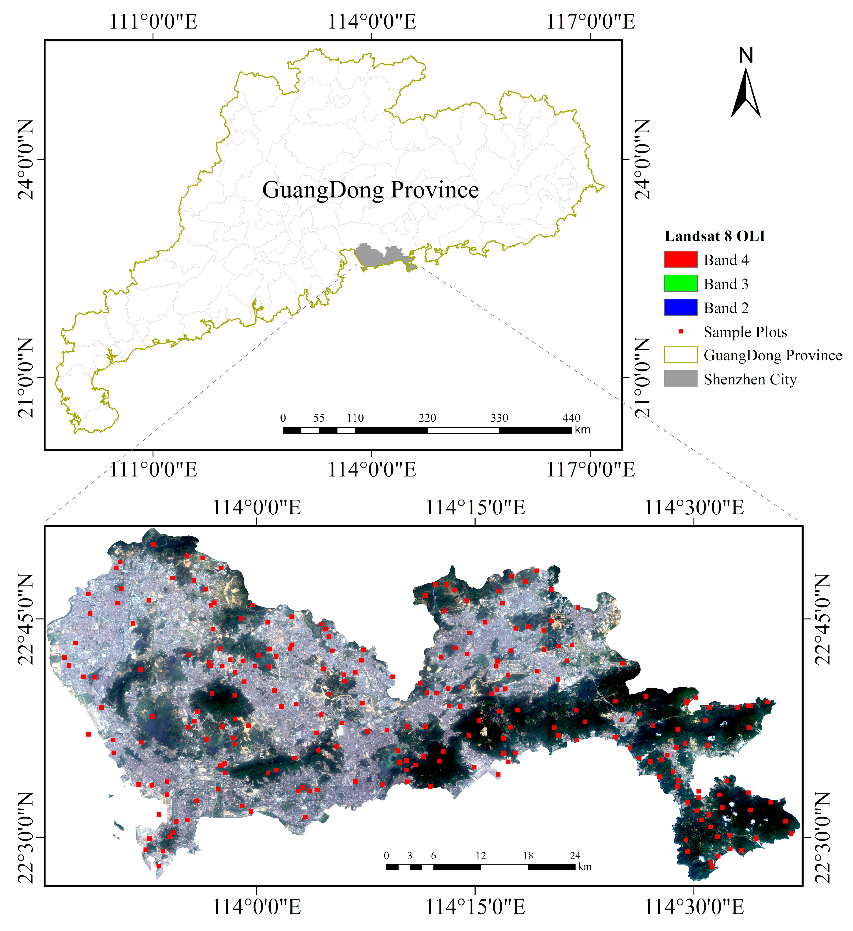
Shenzhen city (113°43′–114°38′ E, 22°24′–22°52′ N) is located in the south-central coastal areas of Guangdong Province, China (Figure 1). It has a subtropical maritime climate with an annual average temperature of 22.4 °C and an annual rainfall of 1933.3 mm. The rainy season is from April to September. The average annual sunshine time is 2120.5 h. The vegetation coverage of the city consists of forest lands, shrublands, grasslands and green roofs. The total area covered by forests and green spaces is 79,700 ha, and approximately 4.88 million trees grow along roads and streets. Deciduous forest stands, mixed coniferous and broad-leaved stands and shrubs were dominant among the forest land cover types. The main conifer species include Masson pine (Pinus massoniana Lamb.), black pine (Pinus thunbergii Parl.) and araucaria (Araucaria cunninghamii Sweet). The main deciduous broad-leaved tree species are Schefflera (Schefflera octophylla (Lour.) Harms), Delonix regia, Albizia julibrissin Durazz., and Kapok (Bombax ceiba L.). The evergreen broad-leaved species include Acacia confuse (Acacia confusa Merr.), Bauhinia (Bauhinia blakeana Dunn), Camphor tree (Cinnamomum camphora (L.) Presl), Ficus microcarpa (Ficus concinna Miq.), and Eucalyptus (Eucalyptus robusta Smith). The main economic forest tree species are Litchi chinensis (Litchi chinensis Sonn.) and Euphoria longan (Dimocarpus longan Lour).
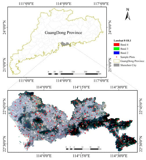
Figure 1.
Location of the study area and the sample plot distribution.
2.2. Satellite Image Acquisition and Processing
In this study, we used Landsat 8-OLI surface reflectance images acquired during the period of June–November 2014. In addition, we used DEM images from two SRTM satellites with a 30-m pixel size. Data acquisition and preprocessing were performed using the GEE API platform, which is based on the JavaScript programming language. We developed a programming script to create all available Landsat imagery collections for the selected time period. An additional advantage was the possibility of use in GEE Landsat 8 images that were already radiometrically corrected and converted to surface reflectance [36,37]. To minimize the cloud problem, we applied the filter to the collection for the purpose of identifying the imagery with less than 10% cloud cover and for avoiding bad collections. After that, using the quality band, we applied a cloud masking function over the images to extract only pixels free from clouds and cloud shadows. Additionally, we collated key information from metadata for each image in the collection (time, solar zenith angle, solar azimuth, etc.). In total, 50 Landsat 8 OLI images were selected and processed in this study. Using the DEM obtained from SRTM data, we calculated the slope and aspect values for every pixel of the study area. Their spatial resolution was 30 m, which corresponded to the Landsat 8 OLI images.
Having these gathered data, for the terrain correction, we performed an illumination correction algorithm as a function in the GEE API, which is based on an empirical rotation model [36]. The results showed that the influence of the shady slope and shadow was greatly eliminated (Figure 2). After applying this function to all images in the collection, we finally reduced the imagery to a composite of median pixel values. The median provided the finest balance between oversaturated and lower pixel values.

Figure 2.
Landsat 8-OLI images (a) before and (b) after terrain illumination correction.
Then, the image was mosaicked and cropped according to the Shenzhen administrative boundary vector layer.
2.3. Measurement of Field Data
In Shenzhen, 234 sample plots were obtained on the principle of stratified random sampling. Using ArcGIS 10.2 software, the total study area was divided into 5 types according to the overall distribution of land types in Shenzhen: forest, urban area, water, grassland, and bare land. The sample plot sizes of the forest, shrub, and grass cover types were 25.82 × 25.82 m, 2 × 2 m, and 1 × 1 m, respectively. The diameter at breast height, height, width of the crown, and height of the branches of each tree in every forest sample plot were recorded. For the shrub sample plot, the species scientific name, ground diameter, total height, and width of the crown of each individual were measured. For the herb samples, the species names, the number of plants (the number of clusters), the average height of the herbs, and the degree of coverage were recorded. To calculate the carbon density per area unit of the plot, the main species in the field survey plot were assigned. Then, the carbon density of each plot (Mg/ha) was calculated using the binary volume table for the main tree species, including soft and hardwood broad-leaved species in Guangdong. All measurements and calculations were performed according to the “Guidelines on carbon accounting and monitoring for afforestation project” [51]. Thus, the total biomass of each plot was calculated. After obtaining the forest biomass (Mg/ha), the forest carbon in each plot was calculated according to the dominant species (group) carbon content table. The carbon sink of shrubs and herbs was obtained based on the model of shrub/herb biomass and height [52] and was then converted to carbon density according to [51].
In total, 234 plots were selected for mapping the carbon density of the urban forests and green spaces in Shenzhen. The statistics in Table 1 show that the mean carbon density among samples that contain carbon was 25.44 Mg/ha and the standard deviation was 20.75 Mg/ha. The obtained urban vegetation carbon density had a large variation coefficient of 81.75%.

Table 1.
Summary statistics of per unit carbon density values (Mg/ha).
2.4. Variables Calculation for Carbon Density Mapping
To choose the most important factors for carbon density modeling, in addition to the original band values of Landsat 8 images, we also used various vegetation indices (NDVI, ARVI, SAVI, TVI, EVI, etc.), the ratio vegetation index of Band-2, the ratio vegetation index of Band-3, and other band ratios [50,53]. In addition, the mean, variance, entropy, second-order matrix, contrast, uniformity, correlation, dissimilarity of each band, and a total of 56 texture features through the texture window of 3 × 3 were considered as potential factors for carbon density modeling. The terrain factors, including the elevation, slope and aspect, and the first four components after the principal component analysis were also extracted. Thus, a total of 273 factors were considered in the modeling. We used ENVI 5.3 software to generate all these variables, and the calculation formulas of the spectral variables are shown in Table 2.

Table 2.
Description of variables used in the study.
2.5. Models for Carbon Density Mapping
MLR, kNN, RF and GWR were frequently used to simulate the relationship between the forest carbon density and spectral variables. MLR needs a significant linear relationship between dependent variables and independent variables, which can measure the impact of multiple variables on prediction. The combination of multiple independent variables is more effective than using only one independent variable to predict carbon density [55]. The general expression of multiple linear regression equation is shown in Equation (1).
where denotes the carbon density (Mg/ha) and X denotes the independent variables.
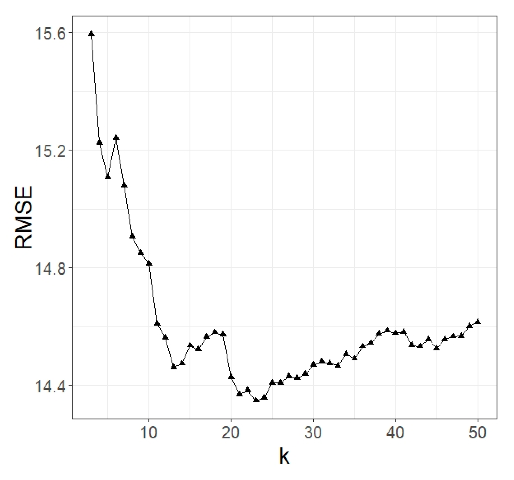
The kNN is established and used to estimate vegetation carbon density. The kNN does not need samples to be specifically distributed, so it is flexible and widely used in vegetation parameter estimation and carbon density mapping [13]. The nearest neighbor k, distance measurement and prediction rules were the factors that strongly affect the estimation results [42]. The k samples nearest to the sample plot to be predicted by spectral distance were searched by the kNN algorithm. The sample plot to be predicted was determined by the specific prediction rules and the attributes of the selected samples [13]. In Shenzhen, we used the Euclidean distance and reciprocal weighting of distance method to predict carbon density (Equation (2)). The initial range of the k value was set as 1–50, and the k with the minimum root mean square error (RMSE) was determined.
where denotes the predicted carbon density at pixel p, denotes the carbon density observation corresponding to the jth sample plot, is the spectral distance from pixel p to the jth sample plot, and k denotes the optimal number of sample plots.
In this study, the kNN model finally obtained the lowest RMSE when k = 23 (Figure 3).
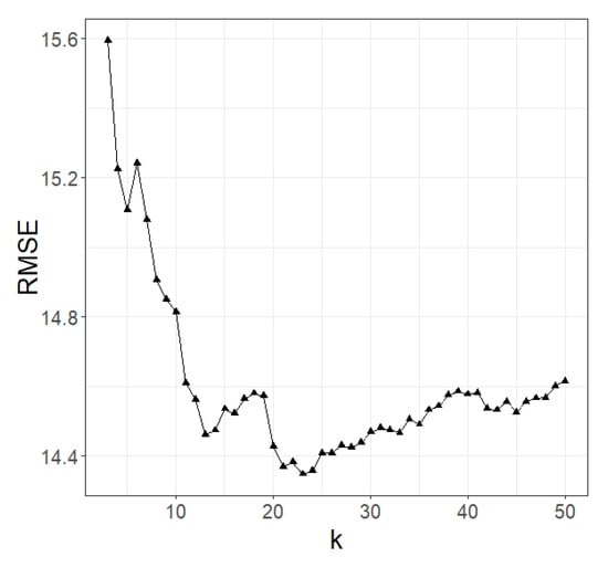
Figure 3.
The RMSE change in the kNN models with the increase of k value.
RF can quickly build a large number of regression trees for prediction. Strong robustness, easy to understand, and insensitive to noise data make it widely used in land change detection and forest parameter estimation [42]. Ntrees which is the number of decision trees and Mtry are important parameters that affect the random forest estimation. Ntrees is set as 500 by default, and Mtry can be set from 1 to the number of variables. In addition, GWR will also be established for comparison of carbon density estimation.
2.6. The OGWLR Model for Carbon Density Estimation
The GWR model combined with logarithmic regression (GWLR) can be used to explore the spatial heterogeneity, which avoids the shortcomings of local variation when deriving spatially invariant regression coefficients [49]. The data should be normalized by Equation (3) before GWR:
Logarithmic transformation to the normalized data must be performed, and a regression model with as the dependent variable must be established. The GWLR model can be written as follows:
where is the location of the target plot, and are the regression coefficients of spatial variation, is the k-th independent variable, and is the estimation error obeying the normal distribution.
The OGWLR model was developed from the GWLR model, and it selected the optimal sampling size by determining the variation in the sample variance and obtained the carbon density prediction value of each sample on the basis of the spatial autocorrelation of the data. First, it determined the maximum spatial autocorrelation distance of all sample points, which was the extraction radius of the model, by statistical analysis of the sample data. Then, a local regression model was established for the pixels inside the extraction circle. Suppose there are N sample points in the circle. We calculate the variance from the sample points with a minimum of 2 to obtain the variance distribution map. When the variance tends to be balanced, the number is the optimal sampling size. In this case, each cell has an optimal sampling size. Finally, the developed model analyzes each cell separately to obtain the final result.
2.7. Model Accuracy Assessment
The leave-one-out cross-validation method (LOOCV) was adopted for the accuracy assessment [56]. This approach is widely used for validation when the field-observed samples are small. This method involves using one field-observed value as a validation sample and the remaining field-observed values as the training samples. We assume N samples and N-1 samples were randomly selected to train the data each time. The average of these N results was used to assess the performance of the model. This process is repeated in all possible combinations to cut the original sample into a validation sample of one field observed value and a training sample [50]. The R2 and RMSE were also used to evaluate the superiority of the models [57]:
where is the measured carbon density, is the estimated carbon density, and n is the sample size. The smaller the RMSE is, the higher the model estimation accuracy is. The larger the determination coefficient (R2) is, the closer the estimate is to the real value.
3. Results
3.1. Correlation Analysis and Selection of Variables
The sample carbon density data after normalization and logarithmic transformation was taken as the dependent variable. In R, the Pearson’s correlation coefficient matrix of the modeling factors and the carbon density was calculated by the corr.test() function of the psycho package [58]. At the significance level of 0.01, 120 variables were significantly associated with carbon density, and the factors with an absolute value of the correlation coefficient greater than 0.600 (p < 0.01) are listed in Table 3. The factor with the highest correlation coefficient of 0.639 was SR536. The stepwise regression method was used to screen out the variable combination for modeling. The variance inflation factor (VIF) was used for testing and eliminating collinearity between variables. Finally, the variable combination significantly related to carbon density and scarce collinearity was used for subsequent modeling and estimation. In Shenzhen, B4, SR536, TVI and SR32 were determined as variables for modeling and estimation.

Table 3.
The absolute correlation coefficients greater than 0.600 between carbon density and the independent variables.
3.2. Result Comparison of the Estimation Models
The MLR, kNN, RF, GWR and OGWLR models were developed using the observed carbon density combined with the Landsat 8 images. The estimated results represented in Table 4 show that there was no significant difference between the estimation accuracy of the kNN and RF. Compared with kNN and RF, the RMSE obtained from GWR decreased by 6.5% and 7.1%, respectively. Additionally, considering the spatial heterogeneity, the accuracy of GWR is slightly improved compared with MLR. However, the OGWLR model achieved the best estimation performance, attaining the highest coefficient of determination (R2 = 0.54) and the lowest RMSE of 13.28 Mg/ha. The results implied that the OGWLR method achieved the best estimation effect, mostly remaining statistically significant (Table 5). Although not statistically significant, RMSE implemented by OGWLR is still 0.14 Mg/ha lower than GWR. The standard deviation of the estimated values obtained by the MLR, kNN, RF and GWR were similar, while the standard deviation of the estimated values obtained by OGWLR was significantly increased. In addition, compared with MLR, kNN and RF, the RMSE acquired by the OGWLR model decreased by 2.4%, 7.5% and 8.0%, respectively.

Table 4.
Accuracies of the forest carbon density estimation models.

Table 5.
The test results (p values) of significant differences among the models based on the absolute residuals between the estimated and observed carbon density values using Student’s t test.
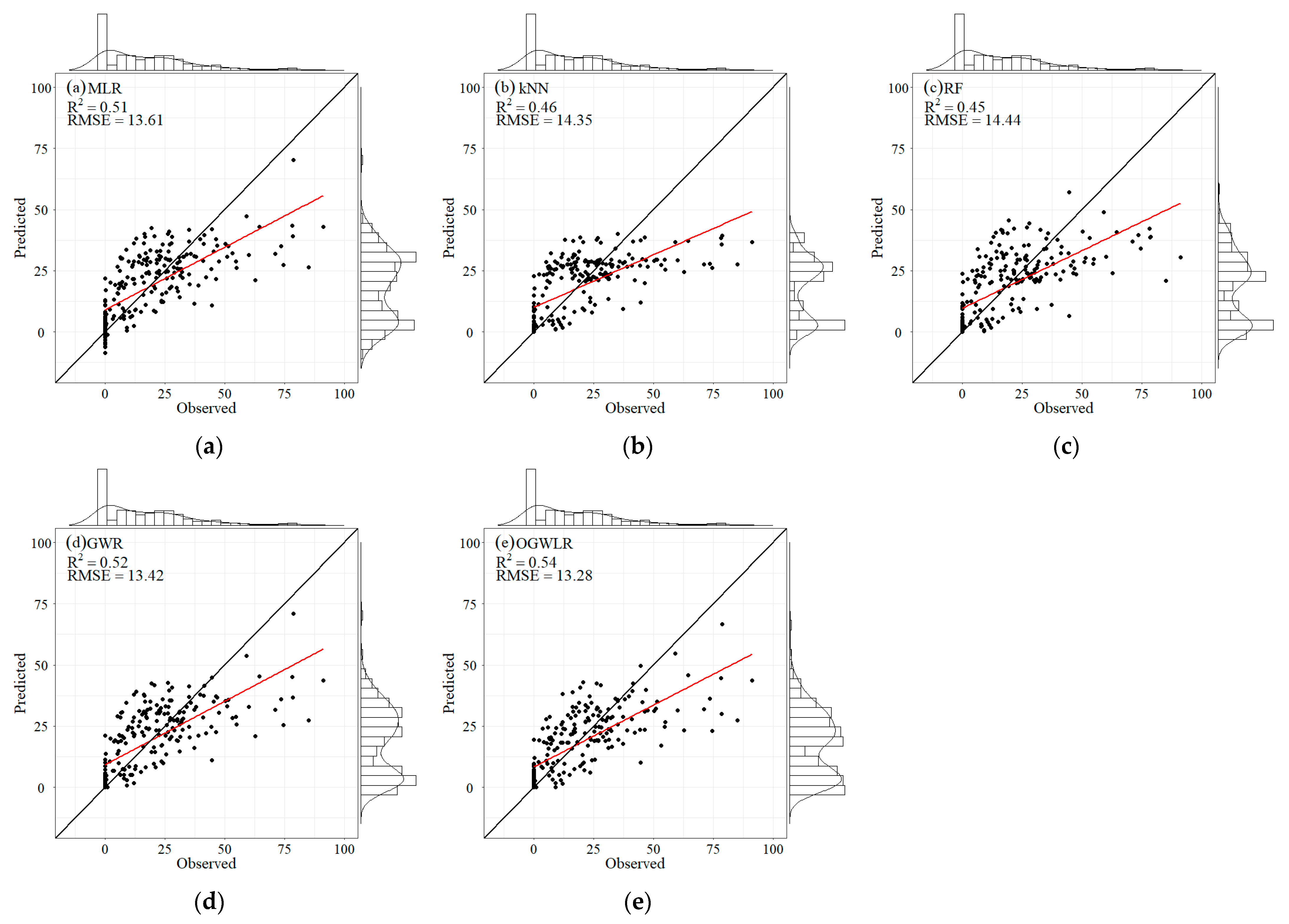
The scatter plots in Figure 4 show the fitting between the observed carbon density and the carbon density predicted by the MLR, kNN, RF, GWR and OGWLR models. The fitting effects of the MLR, kNN, RF, and GWR were similar, with overestimated and underestimated values. However, the predicted values generated by the OGWLR model achieved the best fitting effect with the measured carbon density. The residuals from the OGWLR model were basically distributed and tended to be randomly distributed.
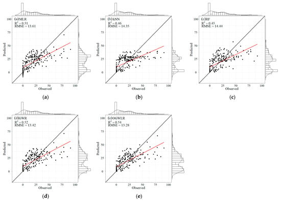
Figure 4.
Scatter plots of (a) the MLR model, (b) the kNN model, (c) the RF model, (d) the GWR model, and the (e) OGWLR model.
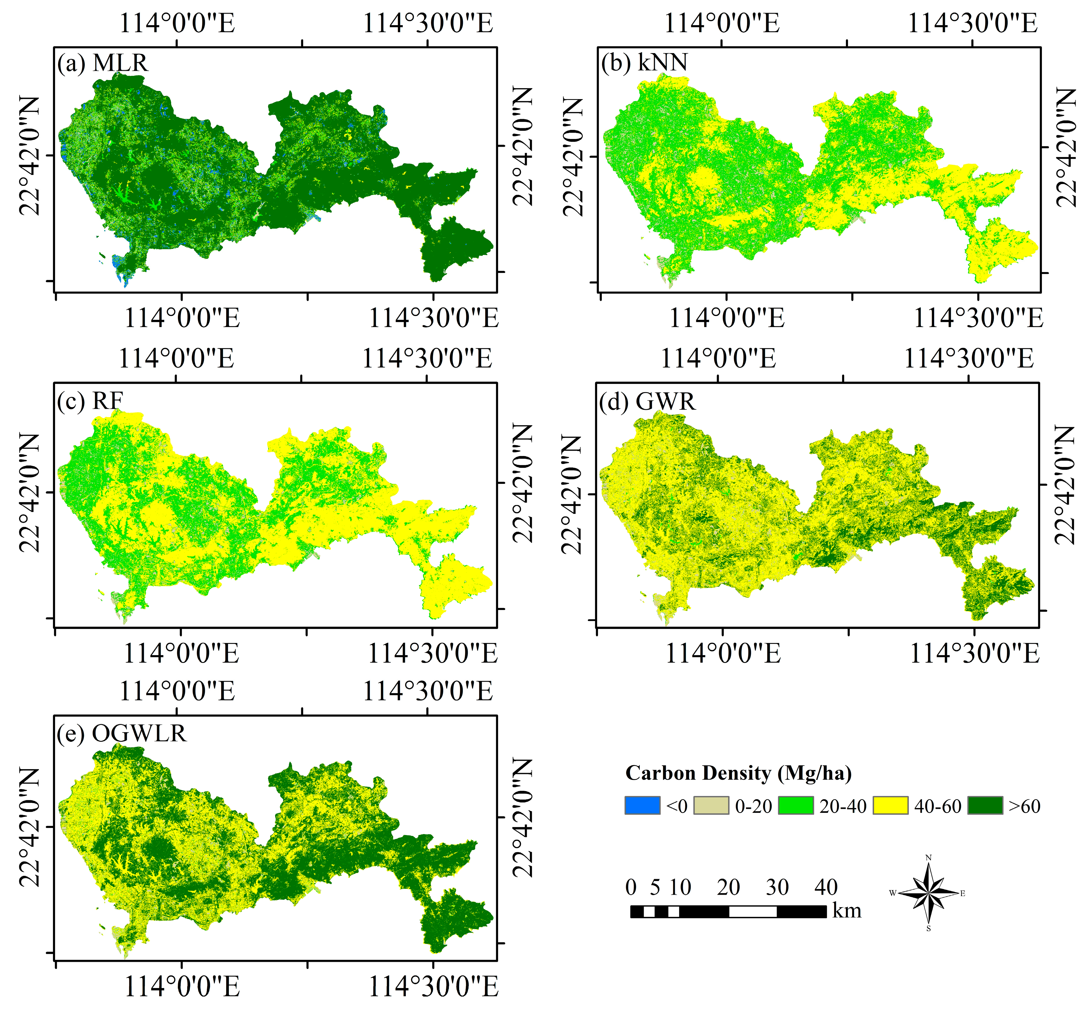
The vegetation carbon density was high within the forest areas in the central and southeastern regions of the study area (Figure 5), with values more than 40 Mg/ha. In urban residential areas and waters, the vegetation carbon density was low. The total carbon storage calculated by MLR, kNN, RF, GWR and OGWLR was 319.6 × 10⁴ Mg, 547.6 × 10⁴ Mg, 567.2 × 10⁴ Mg, 850.8 × 10⁴ Mg and 1098.5 × 104 Mg.
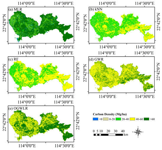
Figure 5.
Carbon density distributions estimated by (a) the MLR model, (b) the kNN model, (c) the RF model, (d) the GWR model, and the (e) OGWLR model.
The spatial distribution of carbon density plotted by the OGWLR model was the closest to the actual distribution of carbon density in Shenzhen, and on the basis of this research, it was the optimal model for the study area.
The OGWLR model uses the same dependent and independent variables as the MLR, kNN, RF and GWR models. The obtained optimal sample size of each pixel can clearly reflect the influence of variance variation on GWR. The scatter plot (Figure 4e) and carbon density map (Figure 5e) showed that the residuals were distributed randomly, and the frequencies of overestimation and underestimation were less than those of the previous four models. The correlation coefficients between the maps acquired by MLR, kNN, RF, GWR and OGWLR are 0.79, 0.90, 0.98 and 0.99 (p < 0.001), respectively, indicating that there is almost no difference between pixels. The improvement of the R2 caused by OGWLR was not significant statistically, while the spatial distribution of carbon density is the most consistent with the actual situation.
4. Discussion
4.1. The OGWLR Model
The GWR method has been widely used in forestry research, especially for the estimation of forest parameters and the classification of land cover types [46,47]. The GWR method can detect the spatial non-stationarity of the model and regression coefficients, but it causes anomalies when it is used for estimating the regression coefficient because of the limitation of the least squares criterion [48]. Propastin et al. [59] improved the GWR method by adding angles to geographically weighted kernel functions to reduce the levels and elevation errors. He adopted this method to estimate the forest biomass in tropical rainforests and obtained an estimation accuracy much higher than that of the traditional GWR model. Zhao et al. [60] reported that climate and topography were the most important factors affecting the growth and distribution of vegetation and proved that the estimation accuracy of GWR was better than that of a multiple linear regression model for LAI estimation.
In this study, the OGWLR model was proposed to explore the spatial distribution of vegetation carbon density. The OGWLR is a local spatial interpolation model developed from the GWR, and it obtained the optimal modeling sample size for each pixel; additionally, carbon density mapping in Shenzhen showed more accurate results than those from the GWLR model. In some studies, the accuracy of forest carbon density estimation using medium-resolution remote sensing images was not satisfactory [18,19,61,62]. The OGWLR method achieved an RMSE of 13.28 Mg/ha using the Landsat 8 images in this study and could be satisfactory at the regional scale. Due to the complexity of urban forest ecosystem, it is difficult to obtain accurate carbon density distribution. The main purpose of this study is to obtain the spatial distribution and trend of carbon density in Shenzhen, and the OGWLR is more consistent with the actual distribution than the traditional methods. Sun et al. [13] estimated the carbon density of the study area by the kNN method and obtained a minimum RMSE value of 18.37 Mg/ha. The determination coefficient acquired by OGWLR model is similar to that of [13] in Shenzhen, but the RMSE is lower.
The low accuracy may be due to the increased sampling size and the spatial variability of the pixels. Based on our results, OGWLR may contribute to improved accuracy. The RMSE achieved by OGWLR was 1.04% smaller than that of GWR, demonstrating the optimal sample size, and could slightly increase the accuracy of the local GWR model. However, compared with GWR, OGWLR has obtained a more reasonable spatial distribution of carbon density, which greatly reduces the overestimation and underestimate of pixel scale.
4.2. Uncertainty, Limitations, and Prospects
This study demonstrated the potential of the OGWLR model for improving the urban vegetation carbon density mapping. However, the estimation error of the vegetation carbon density estimated by OGWLR still has room for improvement. This could be explained by the complex urban landscape and large variation coefficients of the urban vegetation carbon density (81.57%) [63]. A large number of the mixed pixels in Landsat images also contributed to the large relative errors. Therefore, reducing the mixed pixels may improve the urban vegetation carbon density estimation accuracy. Furthermore, in some sample plots, OGWLR obtained a low carbon density and small optimal sampling sizes, which could be caused by insufficient samples for modeling.
The measurement of field sampling data is crucial to obtain the spatial distribution of carbon density of urban vegetation. However, due to the nonnegligible existence of carbon distribution in roadside trees and greenbelts, it is necessary to consider the sample distribution in these areas in order to obtain more reasonable measurement results that can represent the carbon density level in the study area. In addition, shrubs and herbs in the understory of arbor forest are important components of forest carbon storage. In this study, we have considered these factors to reduce the uncertainty caused by the actual sample measurement [64]. Furthermore, the phenomenon of spectral saturation in high vegetation coverage area cannot be ignored. LiDAR can obtain accurate forest information of vertical structure, which has the potential to reduce the saturation and uncertainty of urban forest carbon density estimation [65]. Increasing the number of sample plots of different vegetation types, fusing LiDAR data with optical remote sensing images to extract more accurate vegetation information and considering the spatial heterogeneity of vegetation carbon density distribution may be effective ways to improve the accuracy of urban vegetation carbon density estimation [66].
5. Conclusions
Accurate mapping of the carbon density of urban forest vegetation is critical for climate change monitoring on regional and global scales. Traditional methods often fail to accurately predict the carbon density in a region. In this study, we proposed an OGWLR method for regional carbon density estimation. It was adopted to map the carbon density of urban forest vegetation in Shenzhen. The comparisons between the established methods showed that OGWLR realized the highest prediction accuracy, and its RMSE values were 2.4%, 7.5%, 8.0% and 1.0% smaller than those of MLR, kNN, RF and GWR, respectively. The OGWLR also obtained a more reasonable spatial distribution of carbon density through the local optimal sample size, which clearly shows the impact of variance changes on the local model. The carbon density in the study area was high in the central and western coastal areas and southeastern regions and low in the urban areas, consistent with the actual distribution. Therefore, the proposed OGWLR model is expected to improve the inversion of urban vegetation carbon density. Urban forest has a higher degree of fragmentation than ordinary forest ecosystem, which leads to higher spatial heterogeneity. The OGWLR considers the changes of local samples and can effectively estimate and detect the changes of forest carbon density, which also has application potential for exploring the changes in urban or non-urban areas in wildfire, storm and other disasters.
Author Contributions
Conceptualization and methodology, H.S. and C.L.; validation, F.J. and C.C.; formal analysis, F.J.; investigation, F.J., C.L. and H.S.; draft, F.J., H.S. and M.K.; supervision, H.S.; review, editing, and revision, C.C. and M.K.; funding acquisition, H.S. All authors have read and agreed to the published version of the manuscript.
Funding
This research was funded by the project of the Scientific Research Fund of Hunan Provincial Education Department, grant number 17A225; The Scientific Research Fund of Changsha Science and Technology Bureau, grant number kq2004095; Training Fund of Young Professors from Hunan Provincial Education Department, grant number 90102-7070220090001 and Postgraduate Scientific Research Innovation Project of Hunan Province and Central South University of Forestry and Technology, grant number CX202101005.
Institutional Review Board Statement
Not applicable.
Informed Consent Statement
Not applicable.
Data Availability Statement
Not applicable.
Conflicts of Interest
The authors declare no conflict of interest.
References
- Mauro, G. Rural–Urban Transition of Hanoi (Vietnam): Using Landsat Imagery to Map Its Recent Peri-Urbanization. ISPRS Int. J. Geo-Inf. 2020, 9, 669. [Google Scholar] [CrossRef]
- Dobbs, C.; Escobedo, F.J.; Zipperer, W.C. A framework for developing urban forest ecosystem services and goods indicators. Landsc. Urban. Plan. 2011, 99, 196–206. [Google Scholar] [CrossRef]
- Tubby, K.V.; Webber, J.F. Pests and diseases threatening urban trees under a changing climate. Forestry 2010, 83, 451–459. [Google Scholar] [CrossRef] [Green Version]
- Nowak, D.J. Atmospheric Carbon Reduction by Urban Trees. J. Environ. Manag. 1993, 37, 207–217. [Google Scholar] [CrossRef]
- Zhao, X.; Liu, J.; Hao, H.; Yang, Y. Quantifying the Spatial Heterogeneity and Driving Factors of Aboveground Forest Biomass in the Urban Area of Xi’an, China. ISPRS Int. J. Geo-Inf. 2020, 9, 744. [Google Scholar] [CrossRef]
- Davies, Z.G.; Dallimer, M.; Edmondson, J.L.; Leake, J.R.; Gaston, K.J. Identifying potential sources of variability between vegetation carbon storage estimates for urban areas. Environ. Pollut. 2013, 183, 133–142. [Google Scholar] [CrossRef]
- Luck, M.; Wu, J. A gradient analysis of urban landscape pattern: A case study from the Phoenix metropolitan region, Arizona, USA. Landsc. Ecol. 2002, 17, 327–339. [Google Scholar] [CrossRef]
- Mörtberg, U.M. Resident bird species in urban forest remnants; landscape and habitat perspectives. Landsc. Ecol. 2001, 16, 193–203. [Google Scholar] [CrossRef]
- Ge, M.; Fang, S.; Gong, Y.; Tao, P.; Yang, G.; Gong, W. Understanding the Correlation between Landscape Pattern and Vertical Urban Volume by Time-Series Remote Sensing Data: A Case Study of Melbourne. ISPRS Int. J. Geo-Inf. 2021, 10, 14. [Google Scholar] [CrossRef]
- Jawarneh, R. Modeling Past, Present, and Future Urban Growth Impacts on Primary Agricultural Land in Greater Irbid Municipality, Jordan Using SLEUTH (1972–2050). ISPRS Int. J. Geo-Inf. 2021, 10, 212. [Google Scholar] [CrossRef]
- Nunery, J.S.; Keeton, W.S. Forest carbon storage in the northeastern United States: Net effects of harvesting frequency, post-harvest retention, and wood products. For. Ecol. Manag. 2010, 259, 1363–1375. [Google Scholar] [CrossRef]
- Zeng, W.-S. Development of monitoring and assessment of forest biomass and carbon storage in China. For. Ecosyst. 2015, 1, 467. [Google Scholar] [CrossRef] [Green Version]
- Sun, H.; Qie, G.; Wang, G.; Tan, Y.; Li, J.; Peng, Y.; Ma, Z.; Luo, C. Increasing the Accuracy of Mapping Urban Forest Carbon Density by Combining Spatial Modeling and Spectral Unmixing Analysis. Remote Sens. 2015, 7, 15114–15139. [Google Scholar] [CrossRef] [Green Version]
- Nam, K.; Lee, W.-K.; Kim, M.; Kwak, O.-A.; Byun, W.-H.; Yu, H.; Kwak, H.; Kwon, T.; Sung, J.; Chung, D.-J.; et al. Spatio-temporal change in forest cover and carbon storage considering actual and potential forest cover in South Korea. Sci. China Life Sci. 2015, 58, 713–723. [Google Scholar] [CrossRef] [PubMed] [Green Version]
- Chi, D.; Degerickx, J.; Yu, K.; Somers, B. Urban Tree Health Classification Across Tree Species by Combining Airborne Laser Scanning and Imaging Spectroscopy. Remote Sens. 2020, 12, 2435. [Google Scholar] [CrossRef]
- Lu, D. The potential and challenge of remote sensing-based biomass estimation. Int. J. Remote Sens. 2006, 27, 1297–1328. [Google Scholar] [CrossRef]
- Tian, X.; Su, Z.; Chen, E.; Li, Z.; Van Der Tol, C.; Guo, J.; He, Q. Reprint of: Estimation of forest above-ground biomass using multi-parameter remote sensing data over a cold and arid area. Int. J. Appl. Earth Obs. Geoinf. 2010, 28, 160–168. [Google Scholar] [CrossRef]
- Harkonen, S.; Lehtonen, A.; Eerikäinen, K.; Peltoniemi, M.; Mäkelä, A. Estimating forest carbon fluxes for large regions based on process-based modelling, NFI data and Landsat satellite images. For. Ecol. Manag. 2011, 262, 2364–2377. [Google Scholar] [CrossRef]
- Myneni, R.; Maggion, S.; Iaquinta, J.; Privette, J.; Gobron, N.; Pinty, B.; Kimes, D.; Verstraete, M.; Williams, D. Optical remote sensing of vegetation: Modeling, caveats, and algorithms. Remote Sens. Environ. 1995, 51, 169–188. [Google Scholar] [CrossRef]
- Kay, S.; Hedley, J.D.; Lavender, S. Sun Glint Correction of High and Low Spatial Resolution Images of Aquatic Scenes: A Review of Methods for Visible and Near-Infrared Wavelengths. Remote Sens. 2009, 1, 697–730. [Google Scholar] [CrossRef] [Green Version]
- Muukkonen, P.; Heiskanen, J. Biomass estimation over a large area based on standwise forest inventory data and ASTER and MODIS satellite data: A possibility to verify carbon inventories. Remote Sens. Environ. 2007, 107, 617–624. [Google Scholar] [CrossRef]
- Teillet, P.M.; El Saleous, N.; Hansen, M.C.; Eidenshink, J.C.; Justice, C.O.; Townshend, J.R.G. An evaluation of the global 1-km AVHRR land dataset. Int. J. Remote Sens. 2000, 21, 1987–2021. [Google Scholar] [CrossRef]
- Macfarlane, C. Classification method of mixed pixels does not affect canopy metrics from digital images of forest overstorey. Agric. For. Meteorol. 2011, 151, 833–840. [Google Scholar] [CrossRef]
- Alvarez-Taboada, F.; Paredes, C.; Julián-Pelaz, J. Mapping of the Invasive Species Hakea sericea Using Unmanned Aerial Vehicle (UAV) and WorldView-2 Imagery and an Object-Oriented Approach. Remote Sens. 2017, 9, 913. [Google Scholar] [CrossRef] [Green Version]
- Li, J.; Feng, L.; Pang, X.; Gong, W.; Zhao, X. Radiometric cross Calibration of Gaofen-1 WFV Cameras Using Landsat-8 OLI Images: A Simple Image-Based Method. Remote Sens. 2016, 8, 411. [Google Scholar] [CrossRef] [Green Version]
- Li, Z.; Shen, H.; Li, H.; Xia, G.; Gamba, P.; Zhang, L. Multi-feature combined cloud and cloud shadow detection in GaoFen-1 wide field of view imagery. Remote Sens. Environ. 2017, 191, 342–358. [Google Scholar] [CrossRef] [Green Version]
- Cao, F.; Tzortziou, M. Capturing dissolved organic carbon dynamics with Landsat-8 and Sentinel-2 in tidally influenced wetland–estuarine systems. Sci. Total. Environ. 2021, 777, 145910. [Google Scholar] [CrossRef]
- Lu, D.; Chen, Q.; Wang, G.; Liu, L.; Li, G.; Moran, E. A survey of remote sensing-based aboveground biomass estimation methods in forest ecosystems. Int. J. Digit. Earth 2014, 9, 63–105. [Google Scholar] [CrossRef]
- Potapov, P.; Hansen, M.C.; Stehman, S.V.; Pittman, K.; Turubanova, S. Gross forest cover loss in temperate forests: Biome-wide monitoring results using MODIS and Landsat data. J. Appl. Remote Sens. 2009, 3, 033569. [Google Scholar] [CrossRef]
- Cutler, M.; Boyd, D.; Foody, G.; Vetrivel, A. Estimating tropical forest biomass with a combination of SAR image texture and Landsat TM data: An assessment of predictions between regions. ISPRS J. Photogramm. Remote Sens. 2012, 70, 66–77. [Google Scholar] [CrossRef] [Green Version]
- Lim, K.; Treitz, P.; Wulder, M.; St-Onge, B.; Flood, M. LiDAR remote sensing of forest structure. Prog. Phys. Geogr. Earth Environ. 2003, 27, 88–106. [Google Scholar] [CrossRef] [Green Version]
- Thiel, C.; Schmullius, C. The potential of ALOS PALSAR backscatter and InSAR coherence for forest growing stock volume estimation in Central Siberia. Remote Sens. Environ. 2016, 173, 258–273. [Google Scholar] [CrossRef]
- Vierling, K.T.; Vierling, A.L.; Gould, W.; Martinuzzi, S.; Clawges, R.M. Lidar: Shedding new light on habitat characterization and modeling. Front. Ecol. Environ. 2008, 6, 90–98. [Google Scholar] [CrossRef] [Green Version]
- Mahdianpari, M.; Salehi, B.; Mohammadimanesh, F.; Motagh, M. Random forest wetland classification using ALOS-2 L-band, RADARSAT-2 C-band, and TerraSAR-X imagery. ISPRS J. Photogramm. Remote Sens. 2017, 130, 13–31. [Google Scholar] [CrossRef]
- Seydi, S.; Akhoondzadeh, M.; Amani, M.; Mahdavi, S. Wildfire Damage Assessment over Australia Using Sentinel-2 Imagery and MODIS Land Cover Product within the Google Earth Engine Cloud Platform. Remote Sens. 2021, 13, 220. [Google Scholar] [CrossRef]
- Tamiminia, H.; Salehi, B.; Mahdianpari, M.; Quackenbush, L.; Adeli, S.; Brisco, B. Google Earth Engine for geo-big data applications: A meta-analysis and systematic review. ISPRS J. Photogramm. Remote Sens. 2020, 164, 152–170. [Google Scholar] [CrossRef]
- Tassi, A.; Vizzari, M. Object-Oriented LULC Classification in Google Earth Engine Combining SNIC, GLCM, and Machine Learning Algorithms. Remote Sens. 2020, 12, 3776. [Google Scholar] [CrossRef]
- Li, W.; Niu, Z.; Shang, R.; Qin, Y.; Wang, L.; Chen, H. High-resolution mapping of forest canopy height using machine learning by coupling ICESat-2 LiDAR with Sentinel-1, Sentinel-2 and Landsat-8 data. Int. J. Appl. Earth Obs. Geoinf. 2020, 92, 102163. [Google Scholar] [CrossRef]
- Verrelst, J.; Rivera, J.P.; Veroustraete, F.; Muñoz-Marí, J.; Clevers, J.; Camps-Valls, G.; Moreno, J. Experimental Sentinel-2 LAI estimation using parametric, non-parametric and physical retrieval methods—A comparison. ISPRS J. Photogramm. Remote Sens. 2015, 108, 260–272. [Google Scholar] [CrossRef]
- Wei, C.; Huang, J.; Mansaray, L.R.; Li, Z.; Liu, W.; Han, J. Estimation and Mapping of Winter Oilseed Rape LAI from High Spatial Resolution Satellite Data Based on a Hybrid Method. Remote Sens. 2017, 9, 488. [Google Scholar] [CrossRef] [Green Version]
- Zhu, Y.; Liu, K.; Liu, L.; Myint, S.W.; Wang, S.; Liu, H.; He, Z. Exploring the Potential of WorldView-2 Red-Edge Band-Based Vegetation Indices for Estimation of Mangrove Leaf Area Index with Machine Learning Algorithms. Remote Sens. 2017, 9, 1060. [Google Scholar] [CrossRef] [Green Version]
- Jiang, F.; Smith, A.R.; Kutia, M.; Wang, G.; Liu, H.; Sun, H. A Modified KNN Method for Mapping the Leaf Area Index in Arid and Semi-Arid Areas of China. Remote Sens. 2020, 12, 1884. [Google Scholar] [CrossRef]
- Ahmed, S.; De Marsily, G. Comparison of geostatistical methods for estimating transmissivity using data on transmissivity and specific capacity. Water Resour. Res. 1987, 23, 1717–1737. [Google Scholar] [CrossRef]
- Pardo-Igúzquiza, E. Comparison of geostatistical methods for estimating the areal average climatological rainfall mean using data on precipitation and topography. Int. J. Clim. 1998, 18, 1031–1047. [Google Scholar] [CrossRef]
- Eskelson, B.N.; Anderson, P.D.; Hagar, J.C.; Temesgen, H. Geostatistical modeling of riparian forest microclimate and its implications for sampling. Can. J. For. Res. 2011, 41, 974–985. [Google Scholar] [CrossRef]
- Farber, S.; Páez, A. A systematic investigation of cross-validation in GWR model estimation: Empirical analysis and Monte Carlo simulations. J. Geogr. Syst. 2007, 9, 371–396. [Google Scholar] [CrossRef]
- McMillen, D.P. Geographically Weighted Regression: The Analysis of Spatially Varying Relationships. Am. J. Agric. Econ. 2004, 86, 554–556. [Google Scholar] [CrossRef]
- Brunsdon, C.; Fotheringham, A.S.; Charlton, M.E. Geographically Weighted Regression: A Method for Exploring Spatial Nonstationarity. Geogr. Anal. 2010, 28, 281–298. [Google Scholar] [CrossRef]
- Saefuddin, A.; Widyanings, Y.; Ginting, A.; Mamat, M. Land Price Model Considering Spatial Factors. Asian J. Math. Stat. 2012, 5, 132–141. [Google Scholar] [CrossRef] [Green Version]
- Sun, H.; Wang, Q.; Wang, G.; Lin, H.; Luo, P.; Li, J.; Zeng, S.; Xu, X.; Ren, L. Optimizing kNN for Mapping Vegetation Cover of Arid and Semi-Arid Areas Using Landsat images. Remote Sens. 2018, 10, 1248. [Google Scholar] [CrossRef] [Green Version]
- State Forestry Administration, P.R. China, SFAC. Guidelines on Carbon Accounting and Monitoring for Afforestation Project; China Forestry Publishing House: Beijing, China, 2010. (In Chinese) [Google Scholar]
- Fan, W.; Zhang, H.; Yu, Y.; Mao, X.G.; Yang, J.M. Comparative analysis of three forest biomass estimation models. Chin. J. Plant. Ecol. 2011, 35, 402–410. (In Chinese) [Google Scholar] [CrossRef]
- He, D.-C.; Wang, L. Texture features based on texture spectrum. Pattern Recognit. 1991, 24, 391–399. [Google Scholar] [CrossRef]
- Jiang, F.; Kutia, M.; Sarkissian, A.J.; Lin, H.; Long, J.; Sun, H.; Wang, G. Estimating the Growing Stem Volume of Coniferous Plantations Based on Random Forest Using an Optimized Variable Selection Method. Sensors 2020, 20, 7248. [Google Scholar] [CrossRef] [PubMed]
- Hui, C.L.; Ng, S.F. Predicting Seam Performance of Commercial Woven Fabrics Using Multiple Logarithm Regression and Artificial Neural Networks. Text. Res. J. 2009, 79, 1649–1657. [Google Scholar] [CrossRef]
- Zheng, S.; Cao, C.; Dang, Y.; Xiang, H.; Zhao, J.; Zhang, Y.; Wang, X.; Guo, H. Retrieval of forest growing stock volume by two different methods using Landsat TM images. Int. J. Remote Sens. 2014, 35, 29–43. [Google Scholar] [CrossRef]
- Willmott, C.J.; Ackleson, S.G.; Davis, R.E.; Feddema, J.J.; Klink, K.; LeGates, D.R.; O’Donnell, J.; Rowe, C.M. Statistics for the evaluation and comparison of models. J. Geophys. Res. Space Phys. 1985, 90, 8995–9005. [Google Scholar] [CrossRef] [Green Version]
- Makowski, D. The psycho Package: An Efficient and Publishing-Oriented Workflow for Psychological Science. J. Open Source Softw. 2018, 3, 470. [Google Scholar] [CrossRef]
- Propastin, P. Modifying geographically weighted regression for estimating aboveground biomass in tropical rainforests by multispectral remote sensing data. Int. J. Appl. Earth Obs. Geoinf. 2012, 18, 82–90. [Google Scholar] [CrossRef]
- Zhao, N.; Yang, Y.; Zhou, X. Application of geographically weighted regression in estimating the effect of climate and site conditions on vegetation distribution in Haihe Catchment, China. China. Plant Ecol. 2010, 209, 349–359. [Google Scholar] [CrossRef]
- Michalek, J.L.; French, N.H.F.; Kasischke, E.S.; Johnson, R.D.; Colwell, J.E. Using Landsat TM data to estimate carbon release from burned biomass in an Alaskan spruce forest complex. Int. J. Remote Sens. 2000, 21, 323–338. [Google Scholar] [CrossRef]
- Gleason, C.J.; Im, J. A Review of Remote Sensing of Forest Biomass and Biofuel: Options for Small-Area Applications. GIScience Remote Sens. 2011, 48, 141–170. [Google Scholar] [CrossRef]
- Patenaude, G.; Hill, R.; Milne, R.; Gaveau, D.; Briggs, B.; Dawson, T. Quantifying forest above ground carbon content using LiDAR remote sensing. Remote Sens. Environ. 2004, 93, 368–380. [Google Scholar] [CrossRef]
- Mascaro, J.; Detto, M.; Asner, G.; Muller-Landau, H. Evaluating uncertainty in mapping forest carbon with airborne LiDAR. Remote Sens. Environ. 2011, 115, 3770–3774. [Google Scholar] [CrossRef]
- Neuenschwander, A.L.; Magruder, L.A. The Potential Impact of Vertical Sampling Uncertainty on ICESat-2/ATLAS Terrain and Canopy Height Retrievals for Multiple Ecosystems. Remote Sens. 2016, 8, 1039. [Google Scholar] [CrossRef] [Green Version]
- Lin, X.; Xu, M.; Cao, C.; Dang, Y.; Bashir, B.; Xie, B.; Huang, Z. Estimates of Forest Canopy Height Using a Combination of ICESat-2/ATLAS Data and Stereo-Photogrammetry. Remote Sens. 2020, 12, 3649. [Google Scholar] [CrossRef]
Publisher’s Note: MDPI stays neutral with regard to jurisdictional claims in published maps and institutional affiliations. |
© 2021 by the authors. Licensee MDPI, Basel, Switzerland. This article is an open access article distributed under the terms and conditions of the Creative Commons Attribution (CC BY) license (https://creativecommons.org/licenses/by/4.0/).

