Deep Residual Dual-Attention Network for Super-Resolution Reconstruction of Remote Sensing Images

Abstract

A super-resolution (SR) reconstruction of remote sensing images is becoming a highly active area of research. With increasing upscaling factors, richer and more abundant details can progressively be obtained. However, in comparison with natural images, the complex spatial distribution of remote sensing data increases the difficulty in its reconstruction. Furthermore, most SR reconstruction methods suffer from low feature information utilization and equal processing of all spatial regions of an image. To improve the performance of SR reconstruction of remote sensing images, this paper proposes a deep convolutional neural network (DCNN)-based approach, named the deep residual dual-attention network (DRDAN), which achieves the fusion of global and local information. Specifically, we have developed a residual dual-attention block (RDAB) as a building block in DRDAN. In the RDAB, we firstly use the local multi-level fusion module to fully extract and deeply fuse the features of the different convolution layers. This module can facilitate the flow of information in the network. After this, a dual-attention mechanism (DAM), which includes both a channel attention mechanism and a spatial attention mechanism, enables the network to adaptively allocate more attention to regions carrying high-frequency information. Extensive experiments indicate that the DRDAN outperforms other comparable DCNN-based approaches in both objective evaluation indexes and subjective visual quality.

1. Introduction

With the rapid progress and development of modern aerospace technology, remote sensing images have been widely used in military and civil fields, including agriculture and forestry inspection, military reconnaissance, and urban planning. However, due to hardware limitations and the large detection distance, there is still room for improvement in the resolution and clarity of remote sensing images. Considering the high research cost and long hardware iteration development cycle required to physically improve imaging sensors, it is increasingly important to improve the algorithms used for super-resolution (SR) reconstruction [1] of remote sensing images.

Single-image super-resolution (SISR) technology aims to reconstruct a high-resolution (HR) image from a corresponding low-resolution (LR) image. For aerial remote sensing images, SISR technology can provide richer spatial details by increasing the resolution of LR images. In the past few decades, numerous SISR approaches based on machine learning have been proposed, and these techniques include methods based on neighbor embedding [2], sparse representation [3,4], and local linear regression [5,6]. However, most of these methods use the low-level features of images for SR reconstruction, and the level of ability to represent these features greatly limits the reconstruction effect that is achievable.

With the rapid progress and development of big data and graphics processing unit (GPU) computing capacity, deep convolutional neural networks (DCNNs) have become the dominant approach for achieving success in image processing [7,8,9]. Methods based on DCNNs have shown powerful abilities in the automatic extraction of high-level features from data, providing a highly feasible way to increase the effectiveness of resolution restoration. The basic principle of DCNN-based SR reconstruction methods is to train a model using a dataset that includes both HR images and their corresponding LR counterparts. The model then takes LR images as the input and outputs SR images.

Dong et al. [10] proposed an SR convolutional neural network (SRCNN) that constructs three convolution layers to learn the nonlinear mapping from an LR image to its corresponding HR image. Soon after this, Faster-SRCNN was proposed to accelerate the speed of SRCNN [11]. Shi et al. [12] proposed an efficient sub-pixel convolutional network, which extracts feature information directly from LR images and efficiently reconstructs HR images. Ledig et al. [13] introduced a generative adversarial network (GAN) into the field of SR image reconstruction and produced a super-resolution GAN (SRGAN). In the SRGAN, the input of the generator is an LR image and the output is an HR image, and the discriminator seeks to predict whether the input image is a real HR image or a generated image.

Recently, with the residual network [7] proposed by He et al., many visual recognition tasks have tended to adopt a residual learning strategy for better performance. Kim et al. [14] proposed a very deep SR convolutional neural network (VDSR), which uses residual learning to speed up the convergence of the network while preventing the gradient from disappearing. Soon after this, Kim et al. [15] constructed a deeply recursive convolutional network (DRCN) using recursive modules, which achieves a better reconstruction effect with fewer model parameters. On the basis of DRCN, Tai et al. [16] developed a deep recursive residual network, which combines the residual structure with the recursive module, and this effectively reduces the training difficulty of the deep network. Lim et al. [17] built an enhanced deep SR network (EDSR), and their results showed that increasing the depth of the representation can enhance the high-frequency details of LR images. Zhang et al. [18] proposed a deep residual dense network (RDN), which combines residual learning with dense network connections for SR image reconstruction tasks. Zhang et al. [19] produced a deep residual channel attention network (RCAN), in which a channel attention [20] module is designed to enhance the representation ability of the high-frequency information channel.

With regard to the SR reconstruction of remote sensing images, Lei et al. [21] proposed a new algorithm named local–global combined networks (LGCNet) to learn multilevel representations of remote sensing images, and Dong et al. [22] developed a dense-sampling network to explore the large-scale SR reconstruction of remote sensing images. Inspired by the channel attention mechanism, Gu et al. [23] proposed a residual squeeze and excitation block as a building block for SR reconstruction networks. Furthermore, Wang et al. [24] developed an adaptive multi-scale feature fusion network, in which the squeeze-and-excitation and feature gating unit mechanisms are adopted to enhance the extraction of feature information. These approaches have achieved promising improvements in SR reconstruction of remote sensing images; nonetheless, they still have some deficiencies.

Firstly, as the depth of a CNN increases, the feature information obtained in the different convolutional layers will be hierarchical with different receptive fields. However, most methods only use the features output from the last convolutional layer to realize feature mapping, which neglects the hierarchical features and wastes part of the available information. Secondly, most existing CNN-based methods treat different spatial areas equally, which leads to areas with low-frequency information (smooth areas) being easy to recover while areas with high-frequency details (edges and contours) are more difficult to recover. Moreover, equalization causes the network to use a large amount of computing resources on unimportant features. Thirdly, due to the complex content and richly detailed information contained within remote sensing images, local and global feature information should be considered in the design of the model, and this can lead to learning of multi-level features and improve the reconstruction effect.

Aiming to tackle these issues, this paper proposes a novel aerial remote sensing SR image reconstruction network called a deep residual dual-attention network (DRDAN). This consists of two parts: a global residual learning (GRL) branch and a main residual network (MRN) branch. The GRL branch adopts an upsampling operation to generate the HR counterpart of an LR image directly, which allows the network to avoid learning the complex transformation from one complete image to another. The core of the MRN branch is formed from a stack of basic components called residual dual-attention blocks (RDABs). This network shows superior reconstruction ability and high feature utilization.

The main contributions of this work are as follows:

(1)

We propose a novel approach to SR reconstruction of remote sensing images, DRDAN. This achieves a convenient and effective end-to-end training strategy.

(2)

DRDAN achieves the fusion of global and local residual information, which facilitates the propagation and utilization of image features, providing more feature information for the final reconstruction.

(3)

We propose a modified residual block named RDAB, which contains a local multi-level fusion (LMLF) module and dual-attention mechanism (DAM) module. The LMLF module fuses different level features with the input in the current RDAB. In the DAM module, the channel attention mechanism (CAM) submodule exploits the interdependencies among feature channels and adaptively obtains the weighting information of different channels; the spatial attention mechanism (SAM) submodule pays attention to the areas carrying high-frequency information and encodes which regions to emphasize or suppress; a local residual learning (LRL) strategy is used to alleviate the model-degradation problem due to the deepening of the work, and this improves the learning ability.

(4)

Through comparative experiments with remote sensing datasets, it is clear that, compared with other SISR algorithms, DRDAN shows better performance, both numerically and qualitatively.

The remainder of this paper is organized as follows: Section 2 presents a detailed description of DRDAN, Section 3 verifies its effectiveness by experimental comparisons, and Section 4 draws some conclusions.

2. Methodology

In this section, we will describe the overall architecture and specific details of our proposed DRDAN, including the internal network structure and its mathematical expressions. In particular, each component of RDAB will be illustrated in detail. Then, we give the optimization direction function during the training process of the network. Specifically, we use $I_{\mathrm{LR}}$ and $I_{\mathrm{HR}}$ to represent an LR image and an HR image, respectively. Meanwhile, we define $I_{\mathrm{SR}}$ as the output of our DRDAN.

2.1. Network Architecture

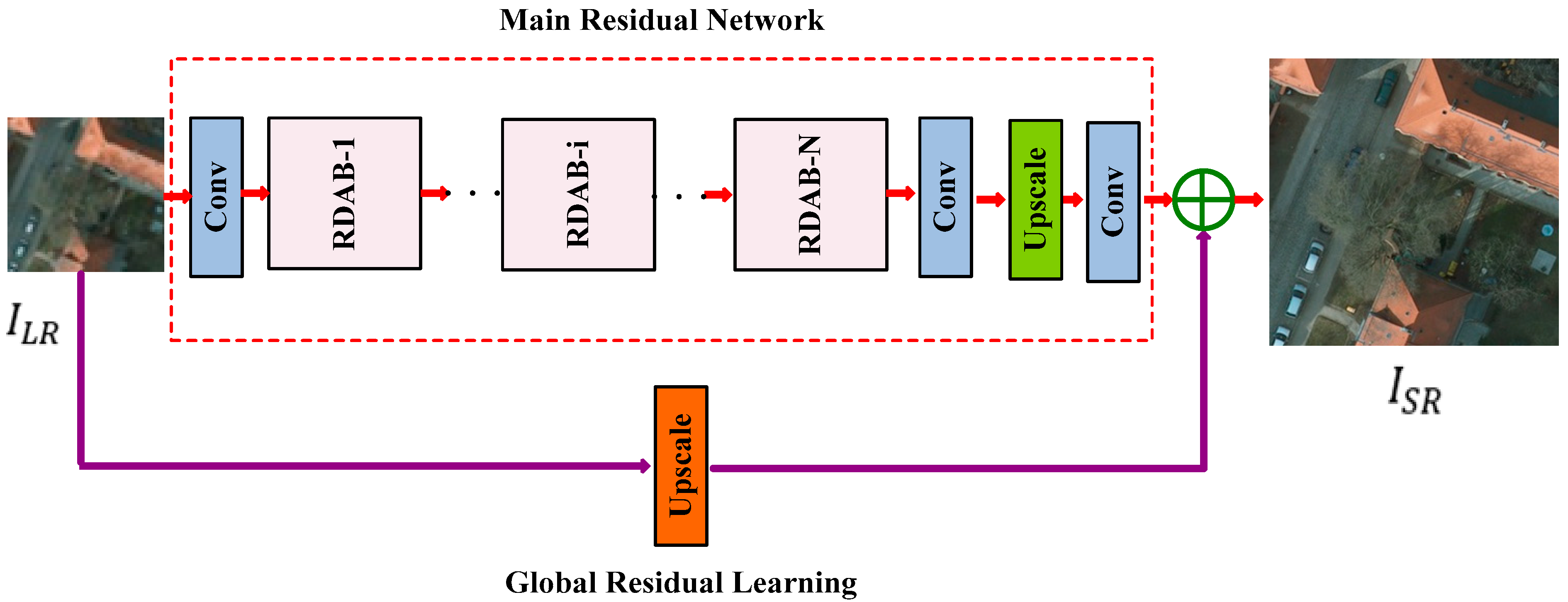
As shown in Figure 1, the DRDAN includes two branches: the GRL branch and the MRN branch. In the GRL branch, we apply bicubic interpolation [25] to make our network learn global residuals inspired by information distillation networks [26]. This process can be formulated as:

$$I_{\mathrm{bicubic}}=H_{\mathrm{bicubic}}\left(I_{\mathrm{LR}}\right),$$

(1)

where $H_{\mathrm{bicubic}}(·)$ denotes the upsampling operator using bicubic interpolation and $I_{\mathrm{bicubic}}$ denotes the image output from the interpolation upsampling operation.

The MRN branch consists of four main parts: shallow feature extraction, deep feature extraction, upsampling, and reconstruction. As with the operation of the EDSR, we extract the shallow features $F_0$ from the LR input by adopting only one convolutional layer:

$$F_0=H_{\mathrm{SF}}\left(I_{\mathrm{LR}}\right),$$

(2)

where $H_{\mathrm{SF}}(·)$ denotes a convolutional layer with kernel size of 3 × 3. The resulting $F_0$ is then used as the input of the deep feature-extraction part with our RDABs. Supposing there are N RDABs, the output feature maps of the n-th RDAB $F_{\mathrm{b},\mathrm{n}}$ can be calculated by:

$$F_{b,n}=H_{\mathrm{RDAB},n}(F_{b,n-1})$$

(3)

where $H_{\mathrm{RDAB},n}(·)$ denotes the operation of the n-th RDAB, and $F_{b,n-1}$ and $F_{b,n}$ are the input and output for the n-th RDAB, respectively. The $H_{\mathrm{RDAB},n}(·)$ operation enables the network to pay more attention to the useful features and suppress useless features, and thus the network can be deepened effectively. The output $F_{b,n}$ is then used for the input of the next part.

After obtaining the deep features of the LR images, we apply an upsampling operation to enlarge the LR feature maps to HR feature maps. Previous methods such as EDSR and RCAN have shown that a pixel shuffle [12] operation has lower computational complexity and higher reconstruction performance than bicubic interpolation calculations. Considering this, we utilized a pixel shuffle operation as our upsampling part, and this operator can be expressed as:

$$F_{\mathrm{up}}=H_{\mathrm{Pixel} \mathrm{Shuffle}}[H_{\mathrm{A}}\left(F_{b,N}\right)],$$

(4)

where $H_{\mathrm{A}}(·)$ denotes a convolutional layer with convolution kernel size of 3 × 3, $H_{\mathrm{Pixel} \mathrm{Shuffle}}[·]$ denotes the upsampling operation by pixel shuffle, $F_{b,N}$ is the output of the last RDAB, and $F_{\mathrm{up}}$ is the upscaled feature maps.

To guarantee that the outputs of the MRN branch and the interpolation upsampling branch have the same number of channels, the upscaled features are then reconstructed via:

$$I_{\mathrm{res}}=H_{\mathrm{rec}}\left(F_{\mathrm{up}}\right),$$

(5)

where $H_{\mathrm{rec}}(·)$ denotes a convolution operation with three output channels and a convolution kernel size of 3 × 3, and $I_{\mathrm{res}}$ denotes the output of the MRN branch.

Finally, the output of DRDAN $I_{\mathrm{SR}}$ is estimated by combining the residual image $I_{\mathrm{res}}$ with the interpolated image $I_{\mathrm{bicubic}}$ using an element-wise summation, which can be formulated as:

$$I_{\mathrm{SR}}=I_{\mathrm{res}}+I_{\mathrm{bicubic}}$$

(6)

2.2. Residual Dual-Attention Block

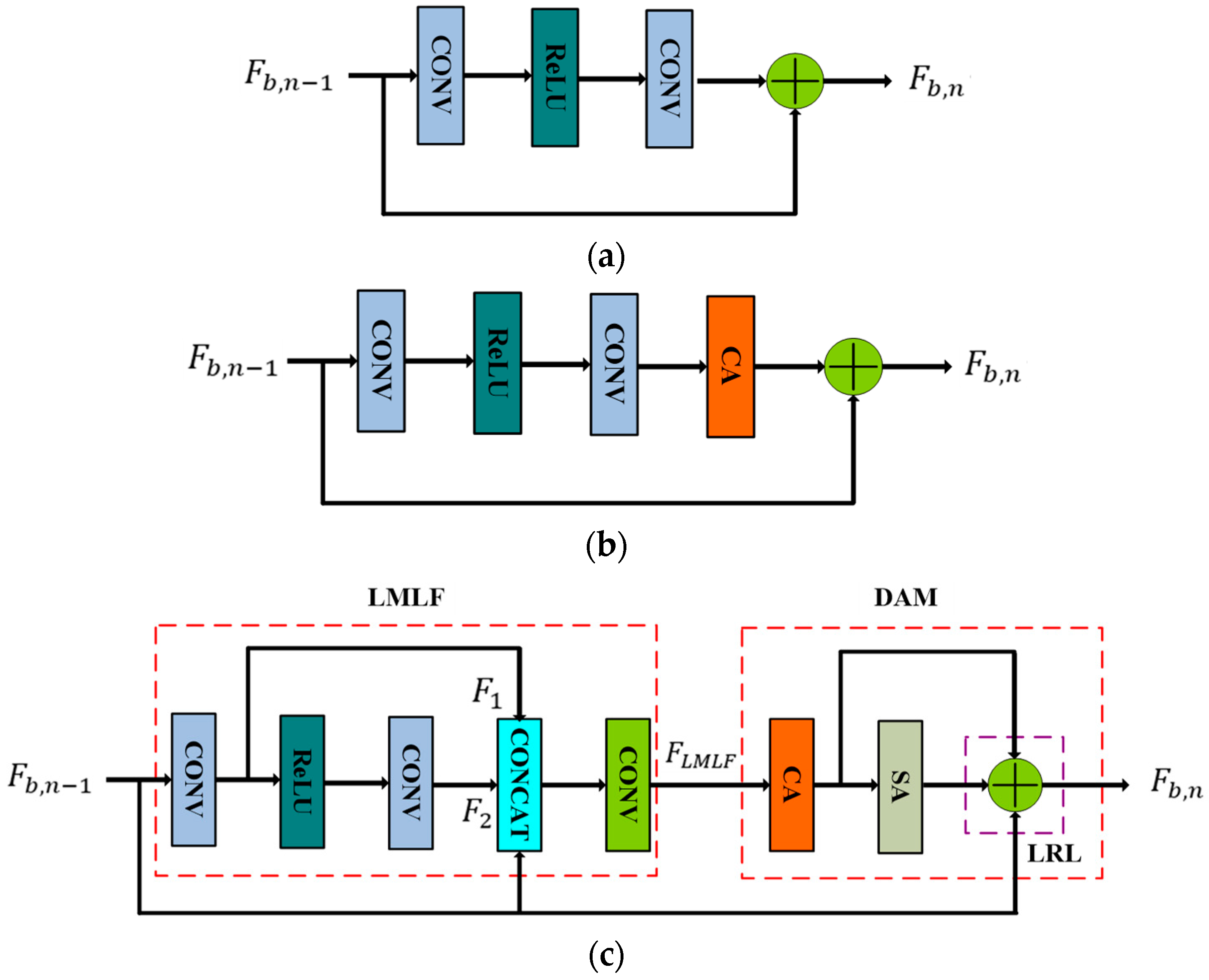
In this section, we will describe the overall structure by using an RDAB. Residual learning strategies can be roughly divided into two types, namely global and local residual learning. Global residual learning only learns the residuals between the input and the output; it thus avoids learning the complex transformation from a complete image to another image, and this effectively reduces the difficulty of model training. As noted in Section 1, VDSR is a classical SISR network based on GRL. Local residual learning means that residual learning is used in stacked convolution layers, and this helps to retain a large amount of image detail information. As shown in Figure 2, we compared our RDAB with some existing residual blocks. Figure 2a–c shows the structures of the residual blocks (RB) in EDSR, the residual channel attention block (RCAB) in RCAN, and the RDAB in DRDAN, respectively. Our RDAB is developed using the LMLF module and the DAM module.

2.2.1. Local Multi-Level Fusion

The feature-extraction module plays an important role in image SR. Extracting and fusing local features with different perceptual scales can obtain more contextual information. By drawing on this idea, we propose an LMLF module to learn more diverse feature information and detailed textures in the RDABs so that the network can learn richer details and enhance feature utilization. The details of this module are shown in Figure 2c. We denote the input of the i-th RDAB as $F_{b,n-1}$. The LMLF module can be formulated as:

$$F_1=f_{1,3}\left(F_{b,n-1}\right),$$

(7)

$$F_2=f_{2,3}\left[\mathrm{ReLU}\left(F_1\right)\right],$$

(8)

$$F_{\mathrm{LMLF}}=f_{3,1}\left[f_{\mathrm{concat}}\left(F_{b,n-1},F_1,F_2\right)\right],$$

(9)

where: $f_{m,n}[·]$ represents the convolution operator, in which m denotes the m-th convolutional layer and n denotes the size of the filters; $f_{\mathrm{concat}}(·)$ represents a concatenation operator; $\mathrm{ReLU}(·)$ denotes a rectified linear unit activation function; $F_1$ and $F_2$ denote the feature maps generated by the first and second convolutional layers in the i-th RDAB, respectively; and $F_{\mathrm{LMLF}}$ is the final output of an LMLF module, and this will be used as the input of the DAM module.

2.2.2. Dual-Attention Mechanism Module

Early CNN-based SR methods mainly focus on increasing the depth and width of the network, and the features extracted by the network are treated equally in all channels and spatial areas. Such methods lack the necessary flexibility for different feature-mapping networks, thus greatly wasting computing resources in practical engineering tasks. The attention mechanism enables the network to pay more attention to information features that are more useful to the target task and suppress useless features. In this way, computing resources can be more scientifically allocated in the feature-extraction process, and the network can be effectively deepened.

The application of attention mechanisms to SISR tasks has been explored using some network architectures such as RCAN and second-order attention network [27], and this has greatly improved the SISR effect. In this paper, we further strengthen the SISR effect by fusing a SAM and a CAM to construct a DAM, which is shown in Figure 2c.

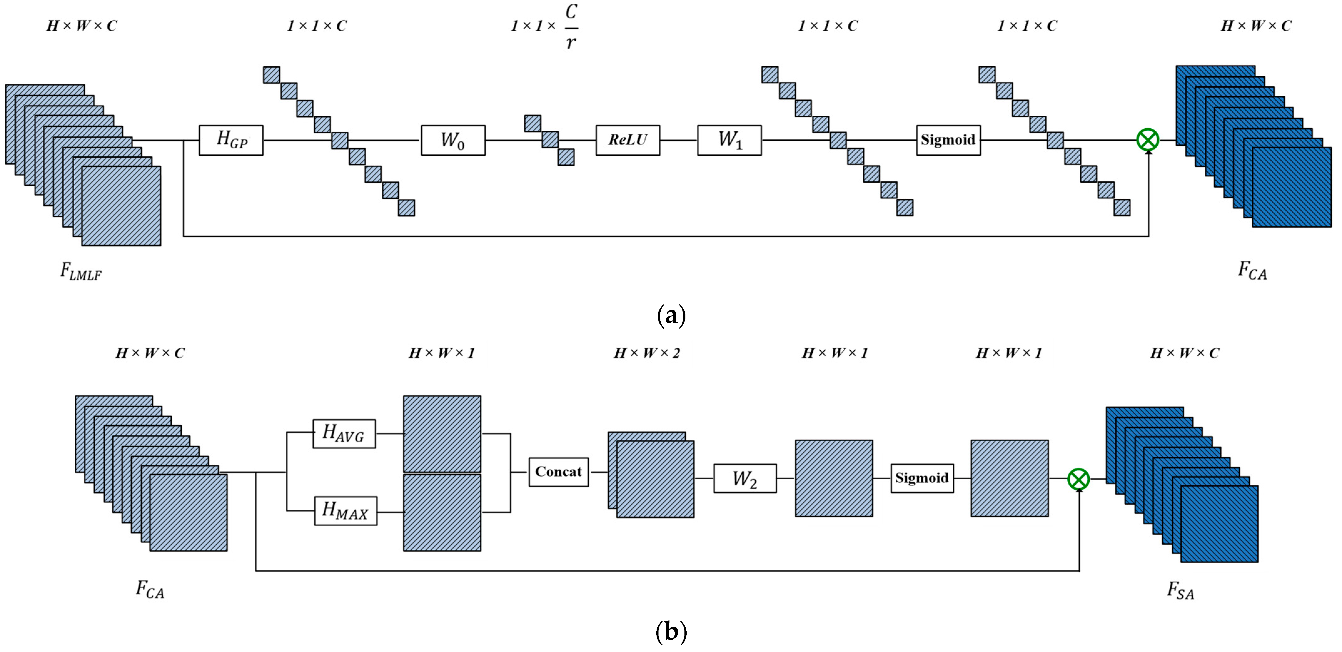
Reference [20] shows that in neural networks, the feature maps extracted by the convolution kernels of different channels will have different abilities in recovering high-frequency detail information. Considering this, we adopt the CAM, in which the representation ability can be improved by explicitly modeling the interconnection of feature channels, adaptively correcting the feature responses of channels, and discriminating between information of different levels of importance. As shown in Figure 3a, we let $F_{\mathrm{LMLF}}=(F_{\mathrm{LMLF}}^1, \cdots , F_{\mathrm{LMLF}}^k,\cdots , F_{\mathrm{LMLF}}^C)$ denote the input feature maps with C channels. The channel feature descriptor $D_{\mathrm{channel}}^k ϵ R^C$ of the k-th feature map $F_{\mathrm{LMLF}}^k$ is determined by global average pooling:

$$D_{\mathrm{channel}}^k=\frac{1}{H\times W}\underset{i=1}{{\displaystyle \sum }^H}\underset{j=1}{{\displaystyle \sum }^W}{F}_{\mathrm{LMLF}}^k\left(i, j\right),$$

(10)

where $F_{\mathrm{LMLF}}^k\left(i, j\right)$ denotes the value at position $\left(i, j\right)$ of $F_{\mathrm{LMLF}}^k$, and W and H denote the width and height of the feature map, respectively. By computing the global average pooling, we can get C channel feature descriptors $D_{\mathrm{channel}}=\left(D_{\mathrm{channel}}^1,\cdots ,D_{\mathrm{channel}}^k,\cdots ,D_{\mathrm{channel}}^C\right)$ corresponding to $F_{\mathrm{LMLF}}=\left(F_{\mathrm{LMLF}}^1, \cdots , F_{\mathrm{LMLF}}^k,\cdots , F_{\mathrm{LMLF}}^C\right)$, respectively. The parameter $D_{\mathrm{channel}}$ describes the importance of different channel features.

After the aggregate operation by global average pooling, we introduce a two-layer perceptron network to fully explore the channel-wise correlation dependencies. The calculation process of the perceptron network is:

$$A_{\mathrm{channel}}=\sigma \left[\mathrm{ReLU}\left(W_0{D}_{\mathrm{channel}}\right)\right],$$

(11)

where: $W_0$ denotes the weight matrix of a convolution layer, which downscales the channel with ratio r; $W_1$ denotes the weight matrix of a convolution layer, which upscales the channel with ratio r; $\sigma [·]$ and $\mathrm{ReLU}(·)$ denote the sigmoid function and ReLU function, respectively; and the output $A_{\mathrm{channel}}=\left(A_{\mathrm{channel}}^1,\cdots ,A_{\mathrm{channel}}^k,\cdots ,A_{\mathrm{channel}}^C\right)$, in which $A_{\mathrm{channel}}^k$ denotes a real value that represents the weight of the k-th channel of $F_{\mathrm{LMLF}}$. The final output of the CAM $F_{\mathrm{CA}}=(F_{\mathrm{CA}}^1,\cdots , F_{\mathrm{CA}}^k, \cdots , F_{\mathrm{CA}}^C$) and $F_{\mathrm{CA}}^k$ is calculated as:

$$F_{\mathrm{CA}}^k=A_{\mathrm{channel}}^k\otimes F_{\mathrm{LMLF}}^k,$$

(12)

where $\otimes$ denotes element-wise multiplication and $F_{\mathrm{CA}}$ denotes feature maps with channel attention.

The LR images contain lots of low-frequency information and a small amount of high-frequency information. The low-frequency information is generally located in smooth areas, which are easy to recover. The high-frequency information, such as edges and contours, is hard to recover. As discussed in [20], it can be found that there is different texture detail information in different spatial locations. However, existing CNN-based methods usually assign the same weight to all spatial locations, which tends to weaken the importance of high-frequency information. Therefore, this work builds a SAM, which emphasizes the attention to high-frequency information areas, thus obtaining a better SR reconstruction effect. As shown in Figure 3b, along the channel axis of $F_{\mathrm{CA}}$, we generate two 2D spatial feature descriptors $D_{\mathrm{spatial}, \mathrm{avg}}$ and $D_{\mathrm{spatial}, \max }$. These are calculated as:

$$D_{\mathrm{spatial}, \mathrm{avg}}\left(i, j\right)=\frac{1}{C}\underset{k=1}{{\displaystyle \sum }^C}{F}_{\mathrm{CA}}^k\left(i, j\right),$$

(13)

$$D_{\mathrm{spatial}, \max }\left(i, j\right)=\underset{k=\left\{1, ···,k,···,C\right\}}{\max }{F}_{\mathrm{CA}}^k\left(i, j\right),$$

(14)

where: $D_{\mathrm{spatial}, \mathrm{avg}}\left(i, j\right)$ and $D_{\mathrm{spatial}, \max }\left(i, j\right)$ denote the average and maximum pooling spatial descriptors at position $\left(i, j\right)$, respectively; $F_{\mathrm{CA}}^k\left(i, j\right)$ denotes the value at position $\left(i, j\right)$ of the k-th feature $F_{\mathrm{CA}}^k$ in $F_{\mathrm{CA}}$; and C is the number of base channels in the feature map.

The concatenated spatial feature descriptors $D_{\mathrm{spatial}}$ are then calculated as:

$$D_{\mathrm{spatial}}=f_{\mathrm{concat}}\left(D_{\mathrm{spatial}, \mathrm{avg}},D_{\mathrm{spatial}, \max }\right),$$

(15)

where $f_{\mathrm{concat}}(·)$ denotes the concatenation operator. The concatenated feature maps $D_{\mathrm{spatial}}$ are convolved by a standard convolution layer, producing the spatial attention map $A_{\mathrm{spatial}}$, which can be formulated as:

$$A_{\mathrm{spatial}}=\sigma [W_2\left(D_{\mathrm{spatial}}\right)],$$

(16)

where $\sigma [·]$ denotes the sigmoid function, and $W_2$ denotes the weight matrix of a convolution layer, which compresses the number of channels of spatial features into one. The output $A_{\mathrm{spatial}}\in R^{H\times W}$ has H × W positions, and $A_{\mathrm{spatial}}\left(i, j\right)$ represents the weight of the feature value at position $\left(i, j\right)$ of $F_{\mathrm{CA}}$. The final output of the SAM $F_{\mathrm{SA}}=\left(F_{\mathrm{SA}}^1,\cdots , F_{\mathrm{SA}}^k, \cdots ,F_{\mathrm{SA}}^C\right)$, and $F_{\mathrm{SA}}^k$ is calculated as:

$$F_{\mathrm{SA}}^k= A_{\mathrm{spatial}}\otimes F_{\mathrm{CA}}^k,$$

(17)

where $\otimes$ denotes element-wise multiplication and $F_{\mathrm{SA}}$ denotes feature maps with spatial attention.

Local residual learning alleviates the model degradation problem of deep networks and improves the learning ability. Furthermore, it also makes the main part of the network pay more attention to the high-frequency information of the LR features. Additionally, short-skip connection can propagate features more naturally from the early layers to the latter layers, which enables better prediction of the pixel density values. To promote the effective delivery of feature information and enhance feature utilization, the final RDAB module output is formulated as:

$$F_{b,n}=F_{b,n-1}+F_{\mathrm{attention}}=F_{b,n-1}+F_{\mathrm{CA}}+F_{\mathrm{SA}}$$

(18)

For a more intuitive understanding of RDAB,

Table 1. RDAB network parameter settings.

Structure Component	Layer	Input	Output
LMLF module	Conv3×3	H × W × 64	H × W × 64
	ReLU	H × W × 64	H × W × 64
	Conv3×3	H × W × 64	H × W × 64
	Concat	H × W × 64, H × W × 64, H × W × 64	H × W × 192
	Conv1×1	H × W × 192	H × W × 64
CAM module	AvgPool	H × W × 64	1 × 1 × 64
	Conv1×1	1 × 1 × 64	1 × 1 × 4
	ReLU	1 × 1 × 4	1 × 1 × 4
	Conv1×1	1 × 1 × 4	1 × 1 × 64
	Sigmoid	H × W × 64	H × W × 64
	Multiple	H × W × 64, 1 × 1 × 64	H × W × 64
SAM module	Mean	H × W × 64	H × W × 1
	Max	H × W × 64	H × W × 1
	Concat	H × W × 1, H × W × 1	H × W × 2
	Conv1×1	H × W × 2	H × W × 1
	Sigmoid	H × W × 1	H × W × 1
	Multiple	H × W × 64, H × W × 1	H × W × 64
LRL module	Sum	H × W × 64, H × W × 64, H × W × 64	H × W × 64

shows the network parameter settings of RDAB, in which: H and W denote the height and width of the feature maps, respectively; Conv3×3 and Conv1×1 denote convolution layers with kernel sizes of 3 × 3 and 1 × 1, respectively; ReLU denotes the rectified linear unit; Sigmoid denotes the sigmoid activation function; AvgPool denotes the global average pooling layer; Mean and Max denote the mean and maximum operations of each point on the feature maps in the channel dimension, respectively; and Multiple and Sum denote the pixel-by-pixel multiplication and addition operations of the feature map, respectively. It should be noted that C is defined as 64 in line with EDSR, and the reduction ratio r is set as 16 in line with RCAN; thus, the convolution layer in channel-downscaling has four filters.

2.3. Loss Fuction

The most widely used loss functions in the field of SR image reconstruction are the L1 and L2 loss functions. The L1 loss function can prevent image distortion and obtain higher test metrics. To perform the same operation as in EDSR, we employ an L1 loss function in our network. We suppose that the given training dataset is ${\{I_i^{\mathrm{LR}}, I_i^{\mathrm{HR}}\}}_{i=1}^N$, where N denotes the number of training samples. The minimum loss function of neural network optimization is then expressed as:

$$L\left(\mathsf{\Theta }\right)=\frac{1}{N}\underset{i=1}{{\displaystyle \sum }^N}\Vert H_{\mathrm{DRDAN}}\left(I_i^{\mathrm{LR}}\right)-I_i^{\mathrm{HR}}\Vert$$

(19)

where $H_{\mathrm{DRDAN}}(·)$ denotes the SR results from the DRDAN network, and $\mathsf{\Theta }=W_i,b_i$ denotes the DRDAN parameter set.

3. Experiments and Results

In this section, we report experiments using remote sensing datasets to evaluate the performance of DRDAN.

3.1. Settings

3.1.1. Dataset Settings

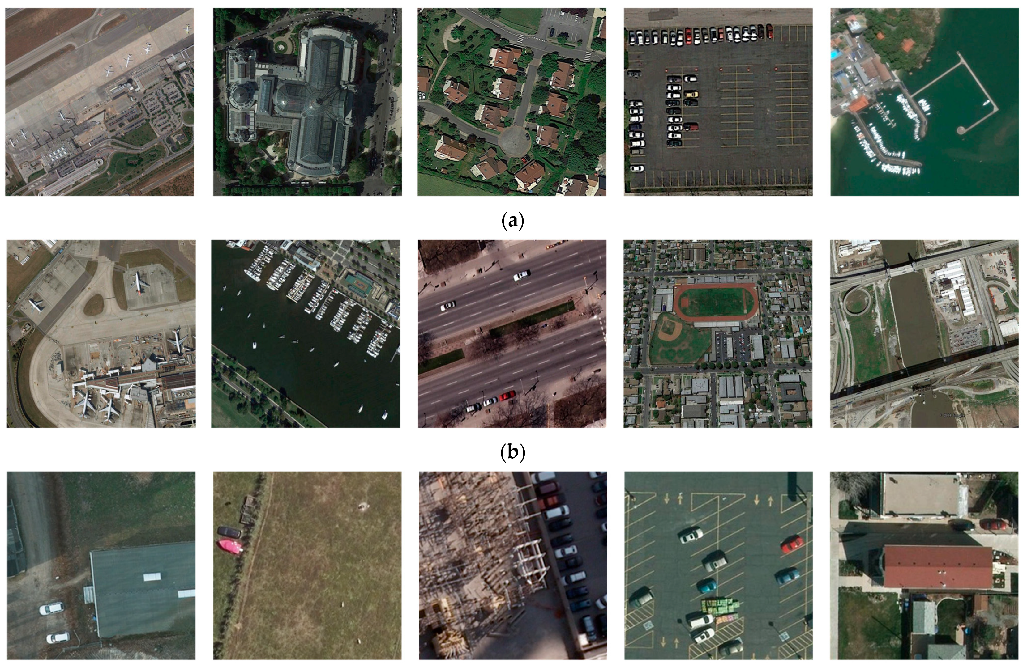
To verify the effectiveness and robustness of our proposed DRDAN, we used 10,000 images from the Aerial Image Dataset (AID) [28] to construct an experimental training dataset. To fully utilize the dataset, the training dataset was augmented via three image-processing methods: (1) horizontal flipping; (2) vertical flipping; and (3) 90° rotation. The trained models were tested on 650 images from the NWPU VHR-10 [29] dataset and 3000 images from the Cars Overhead With Context (COWC) [30] dataset. To obtain LR images, we downsampled the HR images through bicubic interpolation with ×2, ×3, and ×4 scale factors. Some examples of images from each of these datasets are shown in Figure 4.

3.1.2. Evaluation Metrics for SR

We adopted the peak signal-to-noise ratio (PSNR) [31] and structural similarity (SSIM) [31] as the objective evaluation indexes to measure the quality of the SR image reconstruction. The PSNR is one of the most widely used standards for evaluating image quality, and it is generally defined by the mean square error (MSE):

$$M_{\mathrm{MSE}}=\frac{1}{W\times H}\underset{i=1}{{\displaystyle \sum }^H}\underset{j=1}{{\displaystyle \sum }^W}\left[X\left(i,j\right)-Y\left(i,j\right)\right].$$

(20)

The PSNR is expressed as:

$$P_{\mathrm{PSNR}}=20{\log }_{10}(\frac{I_{\max }}{\sqrt{M_{\mathrm{MSE}}}}),$$

(21)

where $X$ denotes an SR image of size W × H, $Y$ denotes an original HR image of size W × H, and $I_{\max }$ denotes the maximum pixel value in the image. The unit of PSNR is dB, and larger $P_{\mathrm{PSNR}}$ values indicate lower distortion and a better SR image reconstruction effect.

The SSIM is another widely used measurement index in SR image reconstruction. It is based on the luminance ($l$), contrast ($c$), and structure ($s$) of samples x and y:

$$l\left(x,y\right)=\frac{2{\mu }_x{\mu }_{y+c_1 }}{{\mu }_x^2+{\mu }_y^2+c_1},$$

(22)

$$c\left(x,y\right)=\frac{2{\sigma }_x{\sigma }_{y+c_2 }}{{\sigma }_x^2+{\sigma }_y^2+c_2},$$

(23)

$$s\left(x,y\right)=\frac{{\sigma }_{xy+c_3}}{{\sigma }_x{\sigma }_y+c_3},$$

(24)

$$\mathrm{SSIM}=\left[l{\left(x, y\right)}^{\alpha }· c{\left(x, y\right)}^{\beta } · s{\left(x, y\right)}^{\gamma }\right],$$

(25)

where ${\mu }_x$ denotes the average value of x, ${\mu }_y$ denotes the average value of y, ${\sigma }_x$ denotes the variance of x, ${\sigma }_y$ denotes the variance of y, and ${\sigma }_{xy}$ represents the covariance of x and y. In general, the values α = β = γ = 1 are set. The range of SSIM is [0, 1]; the closer its value to 1, the greater the similarity between the reconstructed image and the original image, and the higher the quality of the reconstructed image.

3.1.3. Experimental Details

In line with EDSR, we set the number of RDABs as 20. The input LR images were randomly cropped in a patch size of 48 × 48, and the corresponding input HR images with sizes of 96 × 96, 144 × 144, and 192 × 192 were cropped according to the upscaling factors ×2, ×3, and ×4, respectively. To avoid size mismatch during the training process, a zero-padding method was used to ensure that the image size remained consistent during feature delivery. The parameter settings during the training process are shown in

Table 2. Parameter settings during the training process.

Parameter	Setting
Batch size	16
Training epoch number	1500
Optimization method	Adam [32], ${\beta }_1$= 0.9, ${\beta }_2$= 0.999,
	$ϵ={10}^{-8}$
Learning rate (LR)	Initial LR = ${10}^{-4}$,
	.ecreased by a factor of 10 every 500 epochs

. All experiments used the deep-learning framework PyTorch on the Ubuntu 18.04 operating system. Four Nvidia GTX-2080Ti GPUs were used to accelerate the training. The software used included the Python programming language, CUDA 10.1, and cuDNN 7.6.1.

3.2. Results and Analysis

3.2.1. Effect of RDAB

The RDAB is the core of our proposed DRDAN. To further verify the effectiveness of the internal RDAB modules, ablation experiments were implemented on the NWPU VHR-10 and COWC datasets.

Table 3. Ablation experiment results of RDAB on NWPU VHR-10 dataset for SR reconstruction with scale factor ×2. Bold indicates the best performance.

LMLF	CAM	SAM	PSNR	SSIM
⨉	⨉	⨉	34.56139	0.9210
✓	⨉	⨉	34.68720	0.9221
⨉	✓	⨉	34.63267	0.9220
⨉	⨉	✓	34.63908	0.9221
✓	✓	⨉	34.69185	0.9227
✓	⨉	✓	34.68917	0.9225
✓	✓	✓	34.69760	0.9229

and show the effects of this on the LMLF module, CAM module, and SAM module for SR reconstruction with scale factor ×2. Figure 2a shows the structure of the baseline residual block in the ablation experiments. It can be concluded from the tables that the best performance is seen in the model containing the LMLF module, the CAM module, and the SAM module.

The LMLF module aggregates diverse features to enhance the feature utilization of our deep network. To demonstrate the effect of this module, we added the LMLF module to the baseline residual block. The second and the third rows of Table 3 and

Table 4. Ablation experiment results of RDAB on COWC dataset for SR reconstruction with scale factor ×2. Bold indicates the best performance.

LMLF	CAM	SAM	PSNR	SSIM
⨉	⨉	⨉	35.97138	0.9414
✓	⨉	⨉	36.20927	0.9433
⨉	✓	⨉	36.14935	0.9427
⨉	⨉	✓	36.13131	0.9427
✓	✓	⨉	36.23430	0.9434
✓	⨉	✓	36.22175	0.9433
✓	✓	✓	36.23623	0.9434

indicate that this LMLF component can achieve gains of 0.12581 dB and 0.23789 dB for the NWPU VHR-10 and COWC datasets, respectively. This is mainly because the LMLF contributes to the power of the network representation ability.

The DAM consists of both a CAM and a SAM. The CAM explicitly models the interconnections of feature channels, adaptively corrects the feature response of channels, and discriminates between information of different levels of importance. The second and fourth rows of Table 3 and Table 4 indicate that the CAM can achieve gains of 0.07128 dB and 0.17797 dB for the NWPU VHR-10 and COWC datasets, respectively. The SAM enhances the attention paid to high-frequency information areas. The second and the fifth rows of Table 3 and Table 4 indicate that the SAM can achieve gains of 0.07769 dB and 0.15993 dB for the NWPU VHR-10 and COWC datasets, respectively. The third and the last rows of Table 3 and Table 4 indicate that the greatest improvement is achieved when the CAM and SAM are applied together. These comparisons firmly demonstrate the effectiveness of the DAM.

Furthermore, the third, fourth, and sixth rows of Table 3 and Table 4 indicate that ‘LMLF + CAM’ achieves better results than only using LMLF or CAM, respectively. The third, fifth, and seventh rows of Table 3 and Table 4 indicate that ‘LMLF + SAM’ achieves better results than only using LMLF or SAM, respectively. In summary, the experiments show that our RDAB is structured in a rational and efficient way.

3.2.2. Effect of number of RDABs

The RDABs are stacked in the deep feature-extraction part to obtain better feature utilization. We configured the DRDAN with different depths and compared their performance. Specifically, numbers of RDABs ranging from 5 to 25 were used.

Table 5. Performance for different RDAB numbers on NWPU VHR-10 dataset; upper rows show PSNR, and lower rows show SSIM. Bold indicates the best performance.

Scale	RDAB Number
	5	10	15	20	25
×2	34.52445	34.61701	34.66301	34.69760	34.71847
	0.9203	0.9218	0.9224	0.9229	0.9232
×3	31.58175	31.67719	31.72150	31.75685	31.78067
	0.8538	0.8562	0.8573	0.8582	0.8589
×4	29.78881	29.89007	29.92961	29.95408	29.97202
	0.7971	0.8004	0.8017	0.8027	0.8034

and

Table 6. Performance table for different RDAB numbers on COWC dataset; upper rows show PSNR, and lower rows show SSIM. Bold indicates the best performance.

Scale	RDAB Number
	5	10	15	20	25
×2	35.98105	36.12040	36.19822	36.23623	36.26441
	0.9412	0.9425	0.9431	0.9434	0.9437
×3	32.08636	32.26276	32.35570	32.41502	32.46637
	0.8817	0.8845	0.8860	0.8870	0.8877
×4	29.86532	30.03117	30.10245	30.15300	30.18706
	0.8273	0.8311	0.8327	0.8339	0.8346

show the performance with different numbers of RDABs on the NWPU VHR-10 and COWC datasets, respectively. It can be clearly observed that the performance of our DRDAN improves as the number of RDABs increases. This demonstrates that RDAB can be used as a block to train a deep SR reconstruction network.

3.2.3. Effect of GRL

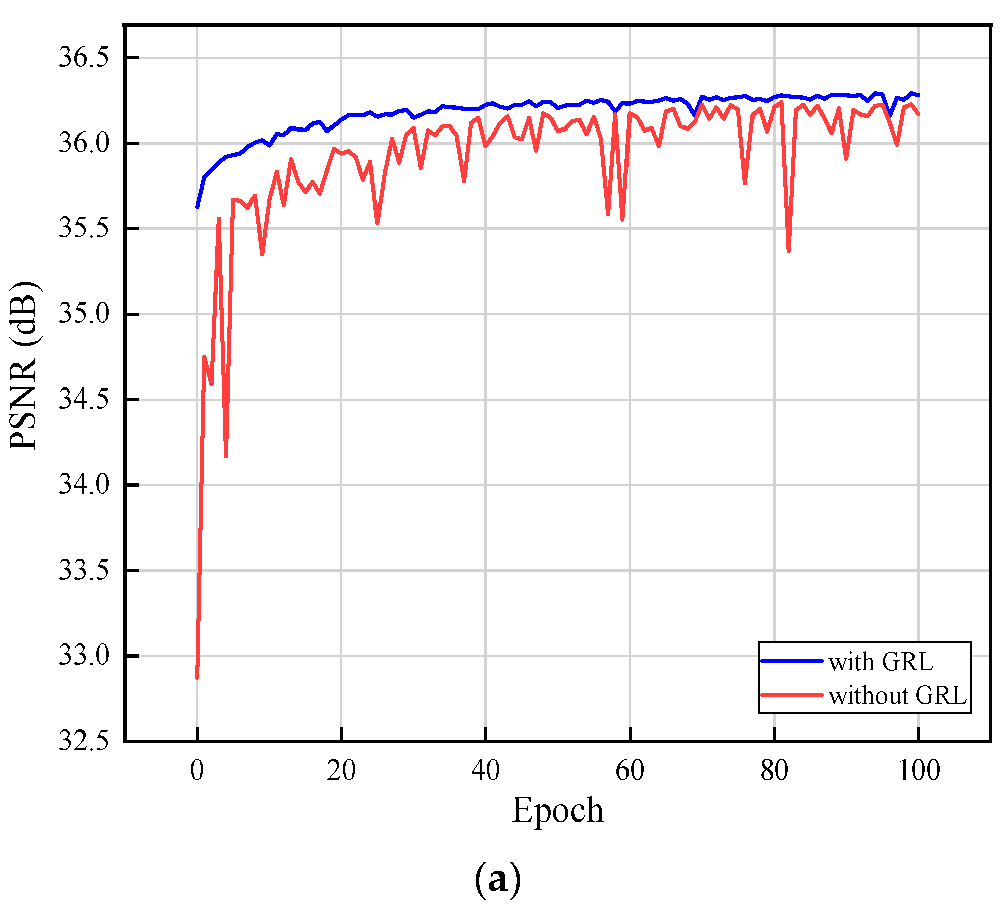
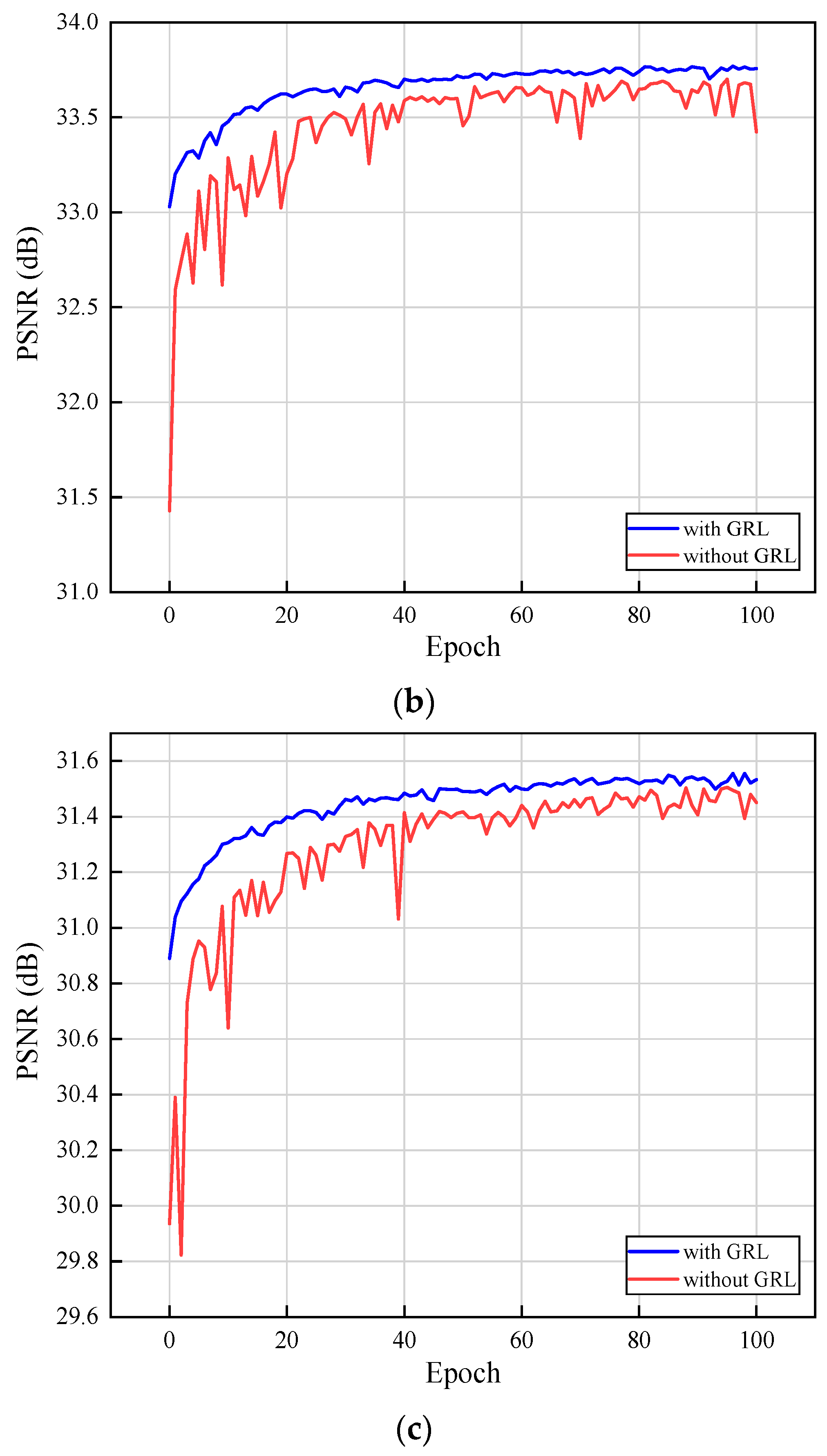
Global residual learning makes the network avoid learning the complex transformation from a complete image to another image; only the residual information needs to be learnt to recover the lost high-frequency details. We now examine the effect of the GRL branch of DRDAN. For rapid testing, we randomly selected ten images from the NWPU VHR-10 dataset to construct a new dataset named FastTest10. Figure 5 shows the performance curve for networks with and without GRL using the FastTest10 dataset in the epoch range 0 to 100. As can be seen from Figure 5, The DRDAN with GRL has a higher PSNR curve and a faster rising speed, which indicates that GRL makes the network converge much faster.

3.2.4. Comparison with Other Approaches

To further verify the advancement and effectiveness of the proposed method, we compared DRDAN with bicubic interpolation, SRCNN, VDSR, local–global combined networks (LGCNet), Laplacian pyramid SR network (LapSRN) [33], EDSR, and wide activation SR (WDSR) [34]. Bicubic interpolation is a representative interpolation algorithm; SRCNN applies a CNN to the image SR task; VDSR adopts residual learning to build a deep network; LGCNet combines global and local features to fully extract multi-level representations of remote sensing images; LapSRN builds a deep CNN within a Laplacian pyramid framework for accurate SR; and EDSR and WDSR are representative versions of deep network architectures with residual blocks. The convolution filters in all the methods were set to 64, and the number of residual blocks in EDSR, WDSR, and DRDAN were all set to 20 to make a fair comparison.

Table 7. Average PSNR and SSIM results of various SISR methods. Upper rows show PSNR, and lower rows show SSIM. Bold indicates the best performance.

Dataset	Scale	Bicubic	SRCNN	VDSR	LGCNet	LapSRN	EDSR	WDSR	Ours
NWPU VHR-10	×2	32.76031	34.03260	34.46067	34.21641	34.24569	34.50910	34.56984	34.69760
		0.8991	0.9136	0.9196	0.9162	0.9169	0.9202	0.9210	0.9229
	×3	29.90444	30.97869	31.46934	31.17537	31.26756	31.57245	31.65636	31.75685
		0.8167	0.8400	0.8517	0.8446	0.8468	0.8539	0.8558	0.8582
	×4	28.28280	29.20195	29.62497	29.34889	29.67748	29.78061	29.87613	29.95408
		0.7524	0.7793	0.7931	0.7841	0.7942	0.7972	0.8003	0.8027
COWC	×2	32.87844	35.05635	35.81885	35.43312	35.48608	35.92949	36.01360	36.23623
		0.9180	0.9341	0.9401	0.9371	0.9375	0.9408	0.9416	0.9434
	×3	29.53540	31.14172	31.89712	31.46921	31.62203	32.04507	32.17758	32.41502
		0.8384	0.8661	0.8788	0.8716	0.8741	0.8811	0.8832	0.8870
	×4	27.72172	28.99814	29.62051	29.23688	29.70046	29.85323	30.00641	30.15300
		0.7725	0.8058	0.8220	0.8123	0.8236	0.8270	0.8305	0.8339

shows the average PSNR and SSIM results of our DRDAN and the compared methods. It can be clearly observed that the proposed DRDAN always yields the best performance. On the NWPU VHR-10 dataset, the DRDAN outperformed the second-best model, WDSR, under factors of ×2, ×3, and ×4 with PSNR gains of 0.12776, 0.10049, and 0.07795 dB, respectively. With the COWC dataset, the average PSNR values that the DRDAN obtained under factors of ×2, ×3, and ×4 were 0.22263, 0.23744, and 0.14659 dB higher than the WDSR. As for SSIM, the super-resolved results from the DRDAN obtained the highest scores. On the NWPU VHR-10 dataset, the SSIM gains of the DRDAN outperformed the second-best model, WDSR, under factors of ×2, ×3, and ×4 by 0.0019, 0.0024, and 0.0024, respectively. On the COWC dataset, the average SSIM values that the DRDAN obtained under factors of ×2, ×3, and ×4 were 0.0018, 0.0038, and 0.0034 higher than the WDSR values, respectively.

3.2.5. Visual Results

In addition to using objective indicators to evaluate the DRDAN, we also examined the reconstruction results qualitatively. Figure 6 shows the reconstructed visual results obtained using DRDAN and the other approaches on COWC test images with three scales, ×2, ×3, and ×4. For a clearer comparison, a small patch marked by a red rectangle is enlarged and shown for each SISR method. As can be observed from the locally enlarged image of Figure 6a, the edges of the red lines obtained using DRDAN are clearer and closer to those in the real image than all of the compared approaches. Figure 6b demonstrates that the DRDAN obtains better perceptual performance with more details and structural textures. Figure 6c shows that the reconstructed vehicle results obtained using DRDAN recover more high-frequency details and obtain sharper edges. It can also be seen from Figure 6 that DRDAN achieves the highest PSNR and SSIM when compared with the other SISR methods. Overall, the DRDAN outperforms other comparative approaches in both objective evaluation indexes and subjective visual quality.

3.2.6. Model Size Analyses

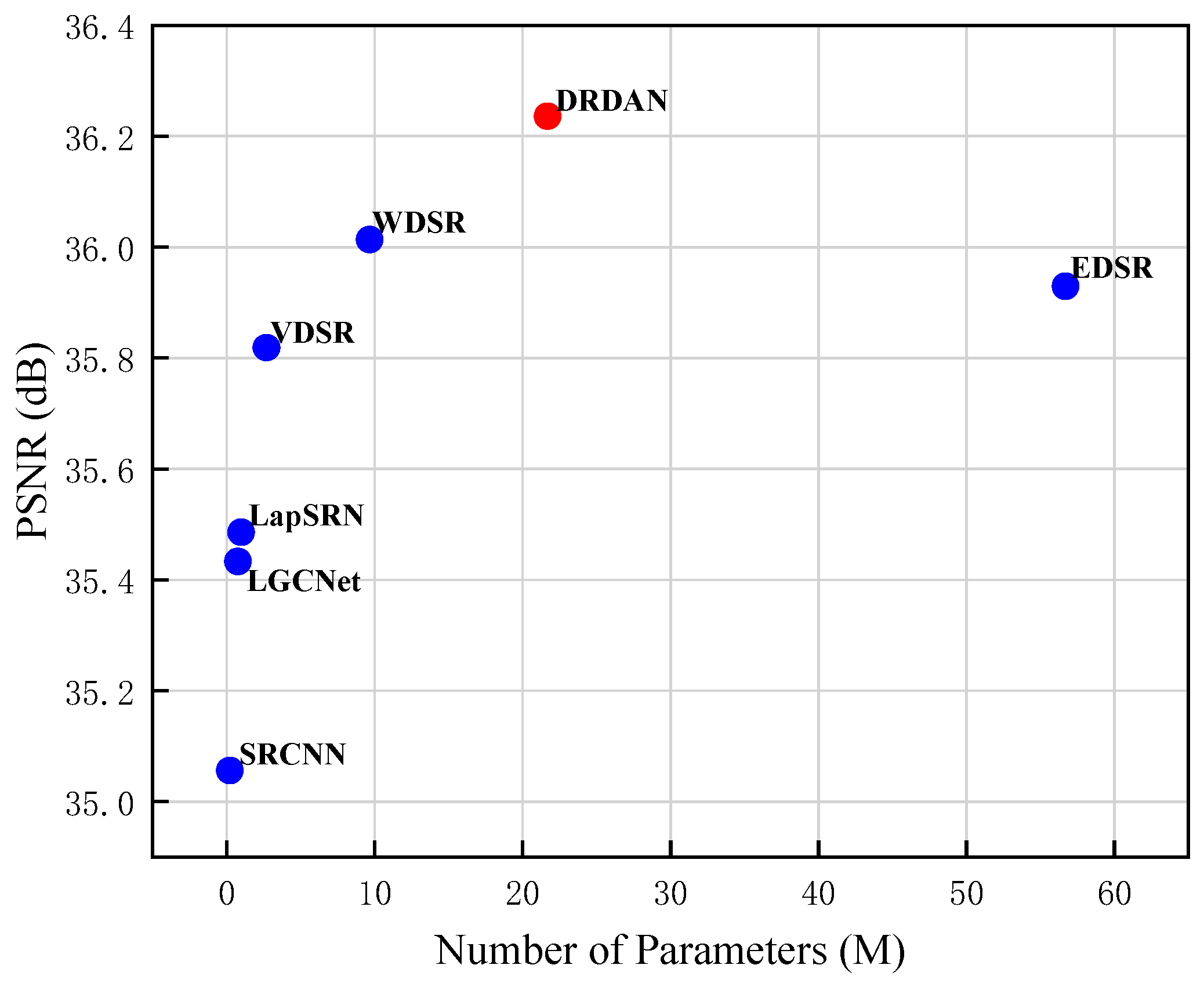
Model size is a critical issue in practical applications, especially in devices with low computing power. For the scaling factor ×2, Figure 7 shows the relationship between the number of parameters of different network structures and the mean PSNR using the COWC test set, where M represents the number of parameters in millions. As we can see from Figure 7, the number of model parameters of DRDAN is less than half of that of EDSR, but the DRDAN performs the best in terms of the PSNR. This finding indicates that our model is structured in a rational and efficient way to achieve a better balance between performance and model size.

4. Conclusions

Existing SR image reconstruction methods suffer from low feature information utilization and equal processing of all spatial regions of an image. Inspired by the idea of residual learning, and combining this with attention mechanism, this paper proposes a deep residual dual-attention network for SR reconstruction of aerial remote sensing images. The main contribution of this paper is the residual dual-attention block, which is constructed as the building block of the deep feature-extraction part of the DRDAN. In the RDAB, we firstly use the local multi-level fusion module to fully extract and deeply fuse the features of the different convolution layers. This module can facilitate the flow of information in the network. After that, the DAM, which includes both a CAM and a SAM, enables the network to adaptively allocate more attention to regions carrying high-frequency information. Extensive experiments indicate that: (1) RDAB is structured in a rational and efficient way, and it can be used as a building block for deep SR reconstruction networks; (2) the global residual learning branch effectively reduces the difficulty of model training and makes the network converge much faster; (3) DRDAN outperforms other comparable DCNN-based approaches, and it can achieve better results with fewer parameters in both objective evaluation indexes and subjective visual quality.

References

1. Glasner, D.; Bagon, S.; Irani, M. Super-resolution from a single image. In Proceedings of the 2009 IEEE 12th International Conference on Computer Vision, Kyoto, Japan, 29 September–2 October 2009; pp. 349–356. [Google Scholar]
2. Chang, H.; Yeung, D.; Xiong, Y. Super-resolution through neighbor embedding. In Proceedings of the 2004 IEEE Computer Society Conference on Computer Vision and Pattern Recognition, Washington, DC, USA, 27 June–2 July 2004; pp. 275–282. [Google Scholar]
3. Yang, J.; Wright, J.; Huang, T.S.; Ma, Y. Image super-resolution via sparse representation. IEEE Trans. Image Process. 2010, 19, 2861–2873. [Google Scholar] [CrossRef] [PubMed]
4. Yang, J.; Wang, Z.; Lin, Z.; Cohen, S.; Huang, T. Coupled dictionary training for image super-resolution. IEEE Trans. Image Process. 2012, 21, 3467–3478. [Google Scholar] [CrossRef] [PubMed]
5. Timofte, R.; Smet, V.D.; Gool, L.V. Anchored neighborhood regression for fast example-based super-resolution. In Proceedings of the IEEE International Conference on Computer Vision, Sydney, NSW, Australia, 1–8 December 2013; pp. 1920–1927. [Google Scholar]
6. Timofte, R.; Smet, V.D.; Gool, L.V. A+: Adjusted Anchored Neighborhood Regression for Fast Super-Resolution. In Proceedings of the Asian Conference on Computer Vision, Singapore, 1–5 November 2014; pp. 111–126. [Google Scholar]
7. He, K.; Zhang, X.; Ren, S.; Sun, J. Deep Residual Learning for Image Recognition. In Proceedings of the IEEE Conference on Computer Vision and Pattern (In CVPR), Boston, MA, USA, 8–11 June 2015; pp. 770–778. [Google Scholar]
8. Ren, S.; He, K.; Girshick, R.; Sun, J. Faster R-CNN: Towards real-time object detection with region proposal networks. In Proceedings of the Advances in Neural Information Processing Systems, Montreal, QC, Canada, 7–12 December 2015; pp. 91–99. [Google Scholar]
9. Long, J.; Shelhamer, E.; Darrell, T. Fully convolutional networks for semantic segmentation. In Proceedings of the IEEE Conference on Computer Vision and Pattern Recognition, Boston, MA, USA, 8–11 June 2015; pp. 3431–3440. [Google Scholar]
10. Dong, C.; Loy, C.; He, K.; Tang, X. Image super-resolution using deep convolutional networks. IEEE Trans. Pattern. Anal. Mach. Intell. 2015, 38, 295–307. [Google Scholar] [CrossRef] [PubMed] [Green Version]
11. Dong, C.; Loy, C.; Tang, X. Accelerating the Super-Resolution Convolutional Neural Network. In Proceedings of the European Conference on Computer Vision, Amsterdam, The Netherlands, 8–16 October 2016; pp. 391–407. [Google Scholar]
12. Shi, W.; Caballero, J.; Huszar, F.; Totz, J.; Aitken, A.; Bishop, R.; Rueckert, D.; Wang, Z. Real-Time Single Image and Video Super-Resolution Using an Efficient Sub-Pixel Convolutional Neural Network. In Proceedings of the IEEE Conference on Computer Vision and Pattern Recognition, Las Vegas, NV, USA, 27–30 June 2016; pp. 1874–1883. [Google Scholar]
13. Ledig, C.; Theis, L.; Huszár, F.; Caballero, J.; Cunningham, A.; Acosta, A.; Aitken, A.; Tejani, A.; Totz, J.; Wang, Z.; et al. Photorealistic single image super-resolution using a generative adversarial network. In Proceedings of the Conference on Computer Vision and Pattern Recognition, Honolulu, HI, USA, 21–26 July 2017; pp. 4681–4690. [Google Scholar]
14. Kim, J.; Lee, J.; Lee, K. Accurate image super-resolution using very deep convolutional networks. In Proceedings of the Conference on Computer Vision and Pattern Recognition, Las Vegas, NY, USA, 27–30 June 2016; pp. 1646–1654. [Google Scholar]
15. Kim, J.; Lee, J.; Lee, K. Deeply-recursive convolutional network for image super-resolution. In Proceedings of the Conference on Computer Vision and Pattern Recognition, Las Vegas, NV, USA, 26 June–1 July 2016; pp. 1637–1645. [Google Scholar]
16. Tai, Y.; Yang, J.; Liu, X. Image super-resolution via deep recursive residual network. In Proceedings of the IEEE Conference on Computer Vision and Pattern Recognition, Honolulu, HI, USA, 21–26 July 2017; pp. 3147–3155. [Google Scholar]
17. Lim, B.; Son, S.; Kim, H.; Nah, S.; Lee, K.M. Enhanced deep residual networks for single image super-resolution. In Proceedings of the IEEE Conference on Computer Vision and Pattern Recognition Workshops, Honolulu, HI, USA, 21–26 July 2017; pp. 1132–1140. [Google Scholar]
18. Zhang, Y.; Tian, Y.; Kong, Y.; Zhong, B.; Fu, Y. Residual dense network for image super-resolution. In Proceedings of the IEEE Conference on Computer Vision and Pattern Recognition, Salt Lake City, UT, USA, 18–23 June 2018; pp. 2472–2481. [Google Scholar]
19. Zhang, Y.; Li, K.; Li, K.; Wang, L.; Zhong, B.; Fu, Y. Image Super-Resolution Using Very Deep Residual Channel Attention Networks. In Proceedings of the European Conference on Computer Vision, Munich, Germany, 8–14 September 2018; pp. 286–301. [Google Scholar]
20. Hu, J.; Shen, L.; Sun, G. Squeeze-and-excitation networks. In Proceedings of the IEEE Conference on Computer Vision and Pattern Recognition, Salt Lake City, UT, USA, 18–22 June 2018; pp. 7132–7141. [Google Scholar]
21. Lei, S.H.; Shi, Z.; Zou, Z. Super-resolution for remote sensing images via local–global combined network. IEEE Geosci. Remote Sens. Lett. 2017, 14, 1243–1247. [Google Scholar] [CrossRef]
22. Dong, X.; Sun, X.; Jia, X.; Xi, Z.; Gao, L.; Zhang, B. Remote sensing image super-resolution using novel dense-sampling networks. IEEE Trans. Geosci. Remote Sens. 2021, 59, 1618–1633. [Google Scholar] [CrossRef]
23. Gu, J.; Sun, X.; Zhang, Y.; Fu, K.; Wang, L. Deep residual squeeze and excitation network for remote sensing image super-resolution. Remote Sens. 2019, 11, 1817. [Google Scholar] [CrossRef] [Green Version]
24. Wang, X.; Wu, Y.; Ming, Y.; Lv, H. Remote Sensing Imagery Super Resolution Based on Adaptive Multi-Scale Feature Fusion Network. Sensors 2020, 20, 1142. [Google Scholar] [CrossRef] [PubMed] [Green Version]
25. Keys, R. Cubic convolution interpolation for digital image processing. IEEE Trans. Acoust. Speech Signal Process. 1981, 29, 1153–1160. [Google Scholar] [CrossRef] [Green Version]
26. Hui, Z.; Wang, X.; Gao, X. Fast and accurate single image super-resolution via information distillation network. In Proceedings of the IEEE Conference on Computer Vision and Pattern Recognition, Salt Lake City, UT, USA, 18–22 June 2018; pp. 723–731. [Google Scholar]
27. Dai, T.; Cai, J.; Zhang, Y.; Xia, S.-T.; Zhang, L. Second-order attention network for single image super-resolution. In Proceedings of the IEEE Conference on Computer Vision and Pattern Recognition, Long Beach, CA, USA, 16–20 June 2019; pp. 11065–11074. [Google Scholar]
28. Xia, G.-S.; Hu, J.; Hu, F.; Shi, B.; Bai, X.; Zhong, Y.; Zhang, L. AID: A benchmark data det for performance evaluation of aerial scene classification. IEEE Trans. Geosci. Remote Sens. 2017, 55, 3965–3981. [Google Scholar] [CrossRef] [Green Version]
29. Cheng, G.; Zhou, P.; Han, J. Learning rotation-invariant convolutional neural networks for object detection in VHR optical remote sensing images. IEEE Trans. Geosci. Remote Sens. 2016, 54, 7405–7415. [Google Scholar] [CrossRef]
30. Mundhenk, T.N.; Konjevod, G.; Sakla, W.A.; Boakye, K. A large contextual dataset for classification, detection and counting of cars with deep learning. In European Conference on Computer Vision; Springer: Cham, Switzerland, 2016; pp. 785–800. [Google Scholar]
31. Horé, A.; Ziou, D. Image quality metrics: PSNR vs. SSIM. In Proceedings of the International Conference on Computer Vision, Istanbul, Turkey, 23–26 August 2010; pp. 2366–2369. [Google Scholar]
32. Kingma, D.P.; Ba, J.L. Adam: A method for stochastic optimization. In Proceedings of the 3rd International Conference on Learning Representations (ICLR 2015), San Diego, CA, USA, 7–9 May 2015. [Google Scholar]
33. Lai, W.; Huang, J.; Ahuja, J.; Yang, M. Deep Laplacian Pyramid Networks for Fast and Accurate Super-Resolution. In Proceedings of the Conference on Computer Vision and Pattern Recognition, Honolulu, HI, USA, 21–26 July 2017; pp. 624–632. [Google Scholar]
34. Yu, J.; Fan, Y.; Yang, J.; Xu, N.; Wang, Z.; Wang, X.; Huang, T. Wide activation for efficient and accurate image super-resolution. arXiv 2018, arXiv:1808.08718. [Google Scholar]
Figure 1. Overview of the DRDAN network structure.
Remotesensing 13 02784 g001
Figure 2. Comparison of the residual blocks of various methods. (a) RB structure of EDSR; (b) RCAB structure of RCAN; (c) RDAB structure of DRDAN.
Remotesensing 13 02784 g002
Figure 3. Overview of the CAM and the SAM. (a) CAM; (b) SAM.
Remotesensing 13 02784 g003
Figure 4. Examples of images from three datasets: (a) AID; (b) NWPU VHR-10; (c) COWC.
Remotesensing 13 02784 g004
Figure 5. Performance curve for DRDAN with and without GRL using FastTest10 dataset with (a) scale factor ×2, (b) scale factor ×3, and (c) scale factor ×4.
Remotesensing 13 02784 g005aRemotesensing 13 02784 g005b
Figure 6. Super-resolution comparison results among the approaches with (a) scale factor ×2, (b) scale factor ×3, and (c) scale factor ×4.
Remotesensing 13 02784 g006
Figure 7. Relationship between number of parameters of different network structures and mean PSNR with COWC test set with scale factor ×2.
Remotesensing 13 02784 g007