Application of a Novel Hybrid Method for Flood Susceptibility Mapping with Satellite Images: A Case Study of Seoul, Korea

Abstract

This paper proposes a novel hybrid method for flood susceptibility mapping using a geographic information system (ArcGIS) and satellite images based on the analytical hierarchy process (AHP). Here, the following nine multisource environmental controlling factors influencing flood susceptibility were considered for relative weight estimation in AHP: elevation, land use, slope, topographic wetness index, curvature, river distance, flow accumulation, drainage density, and rainfall. The weight for each factor was determined from AHP and analyzed to investigate critical regions that are more vulnerable to floods using the overlay weighted sum technique to integrate the nine layers. As a case study, the ArcGIS-based framework was applied in Seoul to obtain a flood susceptibility map, which was categorized into six regions (very high risk, high risk, medium risk, low risk, very low risk, and out of risk). Finally, the flood map was verified using real flood maps from the previous five years to test the model’s effectiveness. The flood map indicated that 40% of the area shows high flood risk and thus requires urgent attention, which was confirmed by the validation results. Planners and regulatory bodies can use flood maps to control and mitigate flood incidents along rivers. Even though the methodology used in this study is simple, it has a high level of accuracy and can be applied for flood mapping in most regions where the required datasets are available. This is the first study to apply high-resolution basic maps (12.5 m) to extract the nine controlling factors using only satellite images and ArcGIS to produce a suitable flood map in Seoul for better management in the near future.

1. Introduction

Globally, flooding and storms as natural disasters have become a serious problem currently, accounting for 67% of all the natural disasters worldwide [1]. Thus, flood susceptibility mapping has recently received significant attention [2,3,4]. In addition, flood damage, which is a significant factor in extreme flood events, is expected to increase in the near future because of climate change [5]. Meanwhile, population increase is expected to severely affect the increase in floods, as it leads to a loss of vegetation owing to construction and increased exposure to flood events. Thus, comprehensive flood management is essential to reduce the effects of floods on human lives. To achieve this aim, a flood susceptibility map can be an effective method, offering information on the probability of flood occurrence, magnitude of the disaster, and location of inundation for flood control.

Flood occurrence is an unpredictable event; therefore, estimating the time of occurrence of a flood and its location is one of the biggest challenges being faced recently. Traditionally, floods are measured using stream gauges installed in water bodies located near populated areas. These gauges constantly monitor the water levels and collect data. Although this is a direct method for determining flood locations, it is costly and time-consuming. Thus, the integration of remote sensing (RS) and geographic information system (ArcGIS) technology has received substantial attention in the field of flood susceptibility mapping. RS can cover different kinds of images at large spatial scales that are critical for depicting geographical characteristics, such as land use/land cover, elevation, slope, and flow direction [6].

The outburst of a flow is affected by many environmental factors including topography, land use, geology, and meteorological parameters, which are useful for preparing flood susceptibility maps. In the last decade, different approaches have been developed for natural hazard mapping like the analytical hierarchy process (AHP) [7], fuzzy logic and frequency ratio [8], genetic algorithm and fuzzy logic [9], hydrological forecasting system [10], variable fuzzy theory [11], decision tree model [12], and machine learning approaches [13]. Of these, the AHP model, as a multi-criteria decision-making (MCDM) method, and geospatial techniques are the simplest methods for determining the flood risk location by using various influencing factors.

AHP is an MCDM method that is implemented in ArcGIS and defines weights for each criterion and sub-criteria. This method uses pairwise comparison matrices (PCMs), which compare all possible pairings of criteria to determine which is the most important. A consistency check is performed in PCM, during which judgment errors are identified and a consistency ratio is calculated. For PCM elements, a number of 1 shows that the criteria are equally important, while a value of 9 indicates that the criterion under examination is exceptionally important in comparison to the other criteria. After determining the most relevant criteria in the flood situation, experts determine the relative relevance of each criterion to the others, which is commonly done on a scale from 1 to 9. Then, the consistency is examined using pairwise comparisons to determine the consistency ratio (CR).

AHP has been commonly used to address various problems because it captures the strategic targets as a collection of weighted parameters, which are then used to score importance of each factor with priorities. It is particularly useful when there is a scarcity of valid data for analysis [14]. For instance, Das [4] used multi sourced environmental flood factors and socio-economic parameters with the AHP approach to prepare high-resolution flood susceptibility, vulnerability, and flood susceptibility maps for the Western Ghat coastal belt, India. In addition, Hwang and Yoon [15] conducted a comprehensive survey of decision-making applications. However, the use of surveys was time-consuming; thus, they were replaced by RS and ArcGIS techniques with thematic layer information. Al-Harbi [16] proposed the use of the AHP model as a decision-making method that considers multiple criteria and presented a comprehensive example to clarify the AHP approach. Allafta [17] used ArcGIS, an RS technique, and AHP to assess groundwater potential zones in the Shatt Al-Arab River basin. In that study, thematic layers were used to prepare basic maps for weighting by using the AHP technique. According to the results, the area was divided into five groundwater potential zones: very poor, poor, moderate, good, and very good.

ArcGIS and RS techniques are useful tools for manipulating and analyzing the information required for determining flood-sensitive areas with high efficiency [2,18]. The combination of AHP with ArcGIS and RS has exhibited good results in previous studies [4,15,19,20]. In these studies, AHP was used to divide regions according to their potential against flood hazards. Chen [21] developed a flood susceptibility map by integrating ArcGIS and AHP techniques in urban and semi-rural areas in central Taiwan. Another flood susceptibility mapping using AHP, and ArcGIS was performed by Sinha [22] in the Kosi River basin, India. To weigh each criterion, the following two most popular techniques are used: direct method of rating [23], which grades each criterion separately and adds all of them into a constant sum, and the use of a pairwise comparison matrix [24], which relies on comparing factors in pairs and expressing the results on a range scale of a constant value. In this study, the pairwise comparison matrix was used in AHP for weighting to compare the results with those obtained previously [25,26], and weights were assigned to the various criteria and their feature classes based on extensive literature reviews and expert knowledge. The use of AHP, ArcGIS, and RS methods in previous studies has yielded comprehensive results [4,16,20,27]. Thus, in the present study, the AHP method was used to develop a flood susceptibility map. Seoul (the capital city of Korea) was selected as a case study area which is located in the central part of the Korean Peninsula between the latitudes of 37°42′ to 37°70′ N and longitudes of 126°76′ to 127°18′ E. It can experience high volume of rain each year which can cause flooding, even though some parts of this city are surrounded by densely forested mountains.

Previous studies have used a combination of directly extracted man-made region maps and ArcGIS maps to develop final flood maps; however, in this study, only high-resolution (12.5 m) satellite images were used to develop flood susceptibility maps. Thus, this study can be considered novel as it uses only maps extracted from ArcGIS and satellite images without direct intervention. Overall, the main objectives of this study were (1) to identify flood potential zones using ArcGIS and AHP and (2) to validate the flood susceptibility map by using a real flood map.

2. Materials and Methods

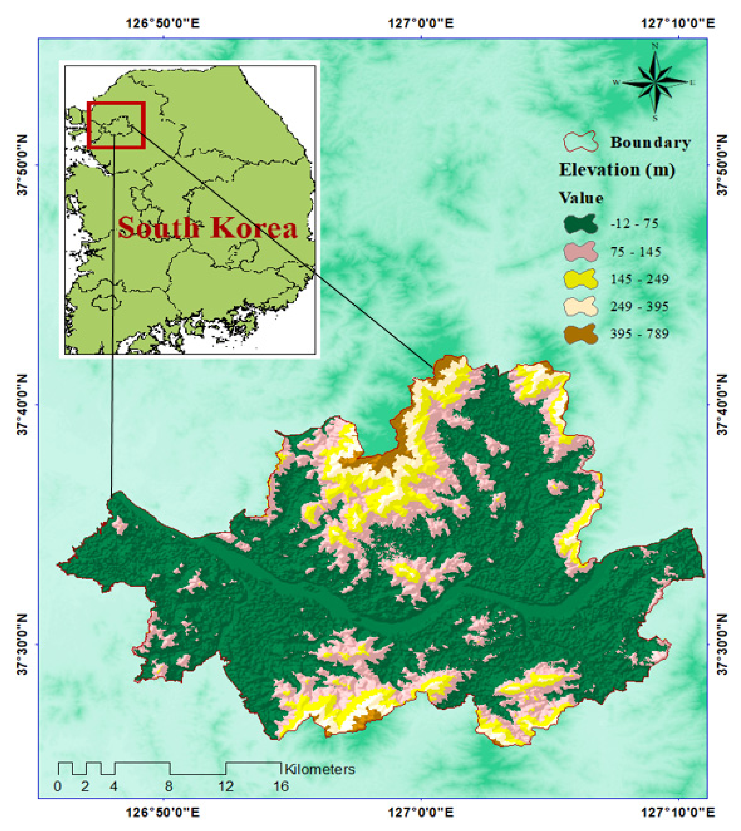
2.1. Study Area

According to government statistics, Seoul is located in the northwestern part of the country with a total area of 605.25 km² [27] and is composed of 25 administrative districts, called GU [28]. The population of Seoul Metropolitan City, which is the world’s tenth largest capital (with more than a quarter of the entire population of South Korea), was approximately 10 million in 2020 [28]. The Han River (Hangang River) is a major river in South Korea and the fourth longest on the Korean Peninsula, after the Amnok (Yalu), Tuman (Tumen), and Nakdong rivers, and crosses Seoul from east to west [29]. The river starts as two smaller rivers in the eastern mountains of the Korean Peninsula, merging near Seoul.

The Han River, located at 126°59′40″ E and 37°33′59″ N, divides the city area into northern and southern portions. It flows through Seoul and then merges with the Rimjin River shortly before flowing into the Yellow Sea. The total length of the Han River is approximately 494 km [30]. Seoul was selected as the case study because more than 80% of rainfall occurs during the monsoon months (July–August) with high potential risks of flood events (Figure 1). Particularly in 2010 and 2011, extreme rainfall wreaked havoc on the city’s southern area, and caused extensive damage to property affected by the flood with worth approximately $65 million [31]. A torrential downpour of 259.5 mm per day on 21 September 2010, caused significant damage to the city center, especially around Gwangwhamun and Cheonggyecheon. Furthermore, on the morning of 27 July 2011, heavy rainfall in the central part of Korea resulted in a rainfall of 164 mm, exceeding the frequency value of over 100 years [28].

The study area’s climate is characterized by dry winter (called “Dwa” in the Köppen climate classification) with four distinct seasons; however, temperature is extremely different between the hottest part of summer and the coldest part of winter. Winters are cold and dry, with the average low temperatures ranging from −6.1 °C (21 °F) to −2.8 °C (27 °F), and temperatures often drop to −17.8 °C (−0 °F). The spring and autumn seasons are warm and dry, with calm weather. During the year, the annual sunshine is 2066 h and the average humidity is 65%. The annual precipitation rate in this area is 1370 mm, with summer accounting for more than 70% of the city’s rainfall.

Due to the high population density and heavy rainfall, the flood occurrence of a large city such as Seoul Metropolitan City becomes a more serious issue; therefore, efficient management to prevent flood events is essential to reduce the considerable cost of disaster recovery. The determination of the main factors influencing flood vulnerability was the first step in preparing the dataset for this study.

2.2. Satellite Images

In this study, the ALOS PALSAR (Phased Array type L-band Synthetic Aperture Radar) sensor was used to derive digital elevation model (DEM) with 12.5 resolution. Regarding this issue, the DEM was downloaded from the website https://search.asf.alaska.edu (accessed date: 20 June 2020). On the other hand, Landsat 8 images (i.e., thematic mapper), with the lowest percentage of cloud cover, were downloaded to generate the land use classification map in ArcGIS using data management tools. By using the DEM as a basic layer, other basic thematic maps (slope, drainage density, topographic wetness index (TWI), flow accumulation, distance from river, and plan curvature) were extracted using ArcGIS. Finally, for interpolation of Landsat 8 images, Erdas Imagine and ArcGIS were used to prepare a land use category map of Seoul, considering google earth images to identify different categories of land use. All above mentioned controlling factors were converted to a raster grid with 12.5 m $\times$ 12.5 m grid cells for application of the AHP model. The flood susceptibility map was prepared after overlaying thematic layers and validating the consistency of the AHP model. A flowchart of the methodology is presented in Figure 2.

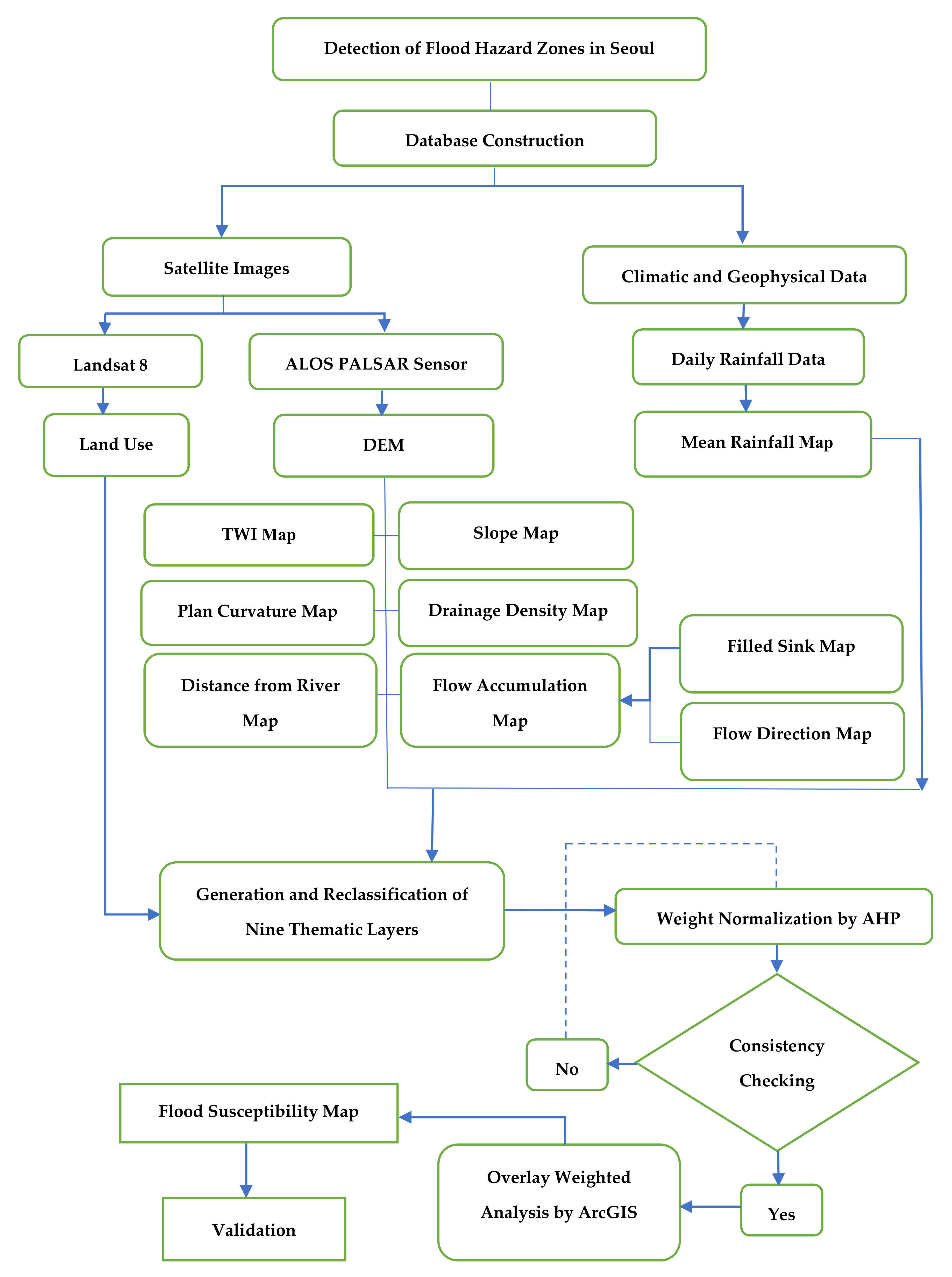
2.3. Delineation of Thematic Layers

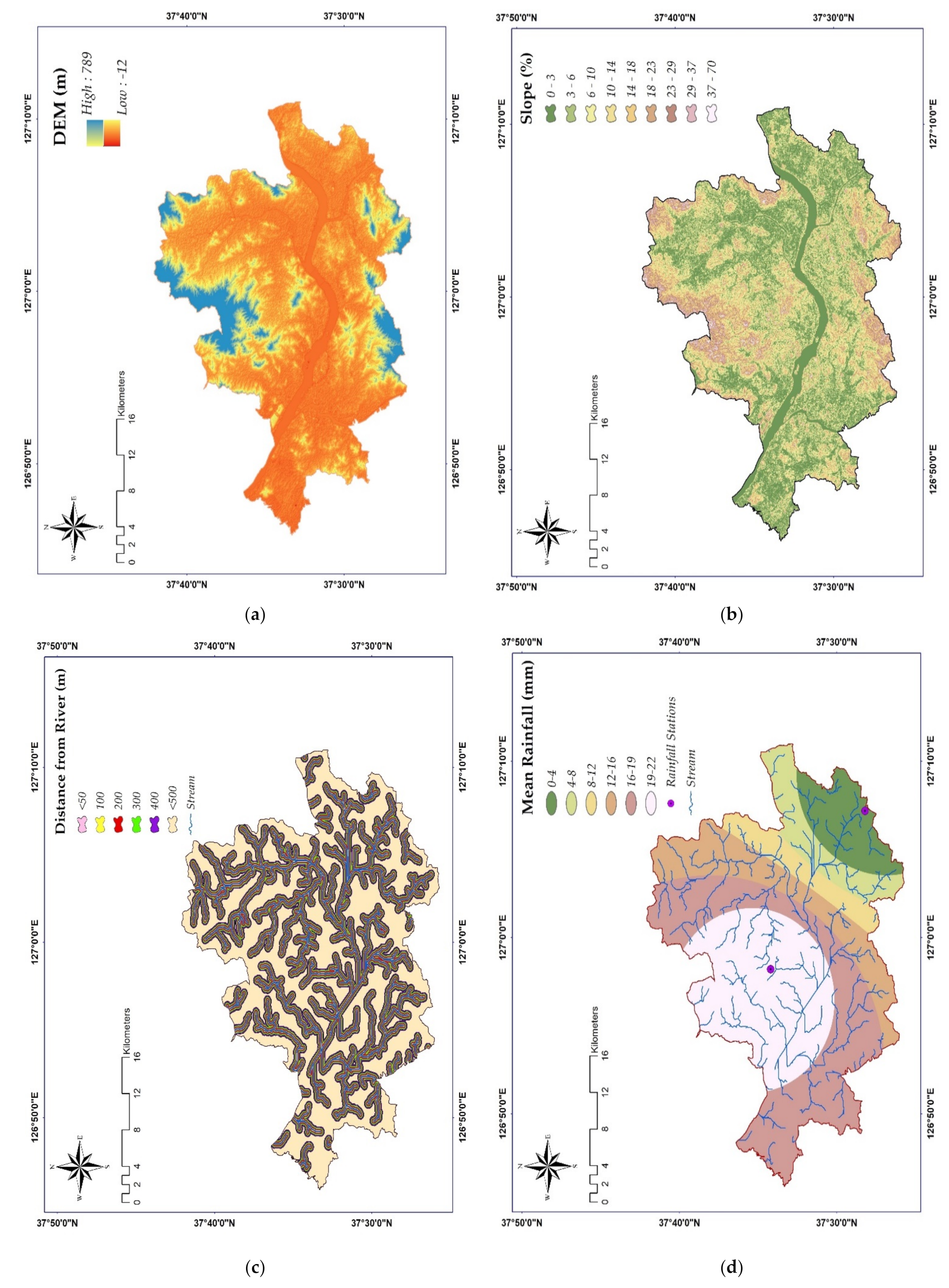
Determining the relevant flood controlling factors is a necessary step in preparing the flood susceptibility map. In this study, nine thematic layers were selected for flood mapping such as DEM, land use, slope, topographic wetness index, plan curvature, river distance, flow accumulation, drainage density, and mean rainfall (Figure 3). As can be seen in this Figure, all thematic layers were extracted from DEM using spatial analyst tools in ArcGIS except a land use map which was prepared from Landsat 8 images with integration of ArcGIS. Taking advantage of the fact that most of the area of Seoul has become an urban area indicated from the new land use map prepared in this study for the year of 2020, the soil map of the area was ignored because of relatively low impact on potential floods. After these layers were prepared, they were converted to a raster format of 12.5-m resolution. Then, the AHP model was used for reclassification using ArcGIS.

2.3.1. DEM

Elevation plays a dominant role in flood susceptibility studies and is used as a basic map for slope, flow accumulation, TWI, plan curvature, and drainage density. As mentioned earlier, a DEM with 12.5-m resolution was obtained from the ALOS PALSAR sensor and was processed in ArcGIS. According to this type of map, floods are less likely to occur in areas far away from the water bodies because of their high elevation. In Figure 3a, high-altitude areas are marked in green and low-altitude areas are marked in dark pink. As areas along the Han River at the central part of Seoul have lower elevation, they are more susceptible to flooding.

2.3.2. Slope

The topographic slope is a common constraint on water velocity and flood strength and is always presented as a percentage or degree. Thus, areas with flat topography and a very low regional slope are more susceptible to flooding when a large volume of water becomes stagnant. As shown in Figure 3b, the southwestern part of Seoul has a slope ranging from 1° to 6°, which is more prone to floods, whereas the northern and southern parts of the city with high slopes have more protection against floods.

2.3.3. Distance from River

The distance from river is another main controlling factor in flood susceptibility mapping which was prepared using the DEM and streamflow. It is an extracted layer from flow accumulation layer using spatial analyst tools in ArcGIS map was prepared using a buffer tool in ArcGIS and classified into six classes in raster format (Figure 3c). According to this type of map, floods are less likely to occur in areas far away from the water.

2.3.4. Mean Rainfall

Among the eight mentioned factors, rainfall seems to have a direct effect on floods. Thus, it is considered to be one of the most crucial factors for flood susceptibility mapping. To prepare the mean rainfall map using ArcGIS, the daily rainfall data for the past 33 years (1987–2019) were downloaded from https://data.kma.go.kr (accessed date: 20 June 2020) for two stations, named Daegokgyo (Latitude 37.47° and Longitude 127.12°) and Seoul (Latitude 37.57° and Longitude 126.97°). This map was extracted using the average monthly rainfall data in ArcGIS. In this study, Inverse Distance Weighting (IDW) was used to extract average monthly rainfall of 33 years. In Figure 3d, dark and light pink areas are more prone to flooding and are located in the center and west part of Seoul.

2.3.5. Flow Accumulation

According to Zhou [32], one of the most significant factors that has been commonly measured and used in various studies is flow accumulation, which represents the total amount of water that has flown from the upstream areas to a particular point within the catchment. This map was extracted using spatial analyst tools in ArcGIS. A higher flow accumulation value indicates a greater likelihood of water accumulation and thus a greater likelihood of flooding. In Figure 3e, the central part of Seoul (near the Han River) shows a high amount of flow accumulation.

2.3.6. TWI

This is a secondary topographical attribute that depicts the spatial distribution of wetness conditions and can be described as [33]:

$$\mathrm{TWI}=\mathrm{In}\left(\frac{\mathsf{\alpha }}{\tan \mathsf{\beta }}\right)$$

(1)

where α represents the upslope area per unit contour length through a point and tan β is the slope angle at that point. In this study, TWI was extracted using map algebra tool in ArcGIS and divided into four classes by using three basic maps: DEM, TWI, and flow accumulation (Figure 3f). TWI has a direct relation with flood events, implying that areas with a higher TWI are more vulnerable to flooding.

2.3.7. Plan Curvature

The plan curvature is the curvature in a horizontal plane and is also known as the curvature of a hypothetical contour line that passes through a particular cell. Cells with concave contours have a positive plan curvature, whereas those with convex contours have a negative plan curvature. The plan curvature can be analyzed to extract useful geomorphological details [34]. The concave, flat, and convex planes are the three types of plan curvatures used in this study (Figure 3g). A negative value indicates a concave shape, a positive value indicates a convex shape, and a value close to zero indicates a flat field. This map was created using 3D analyst tools in ArcGIS. The negative value has the highest weight in the heightening curvature map because flood events are more common.

2.3.8. Drainage Density

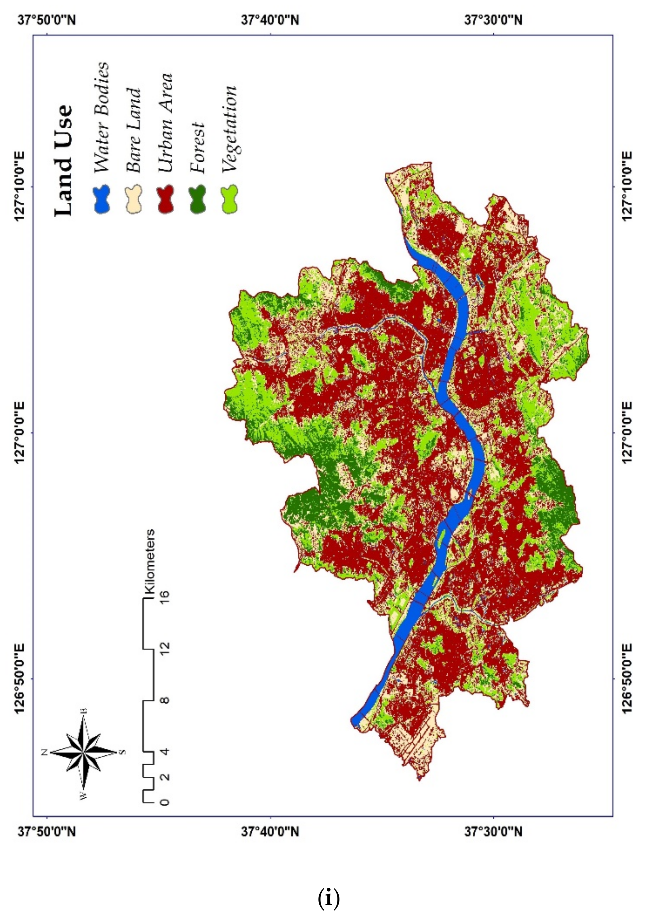
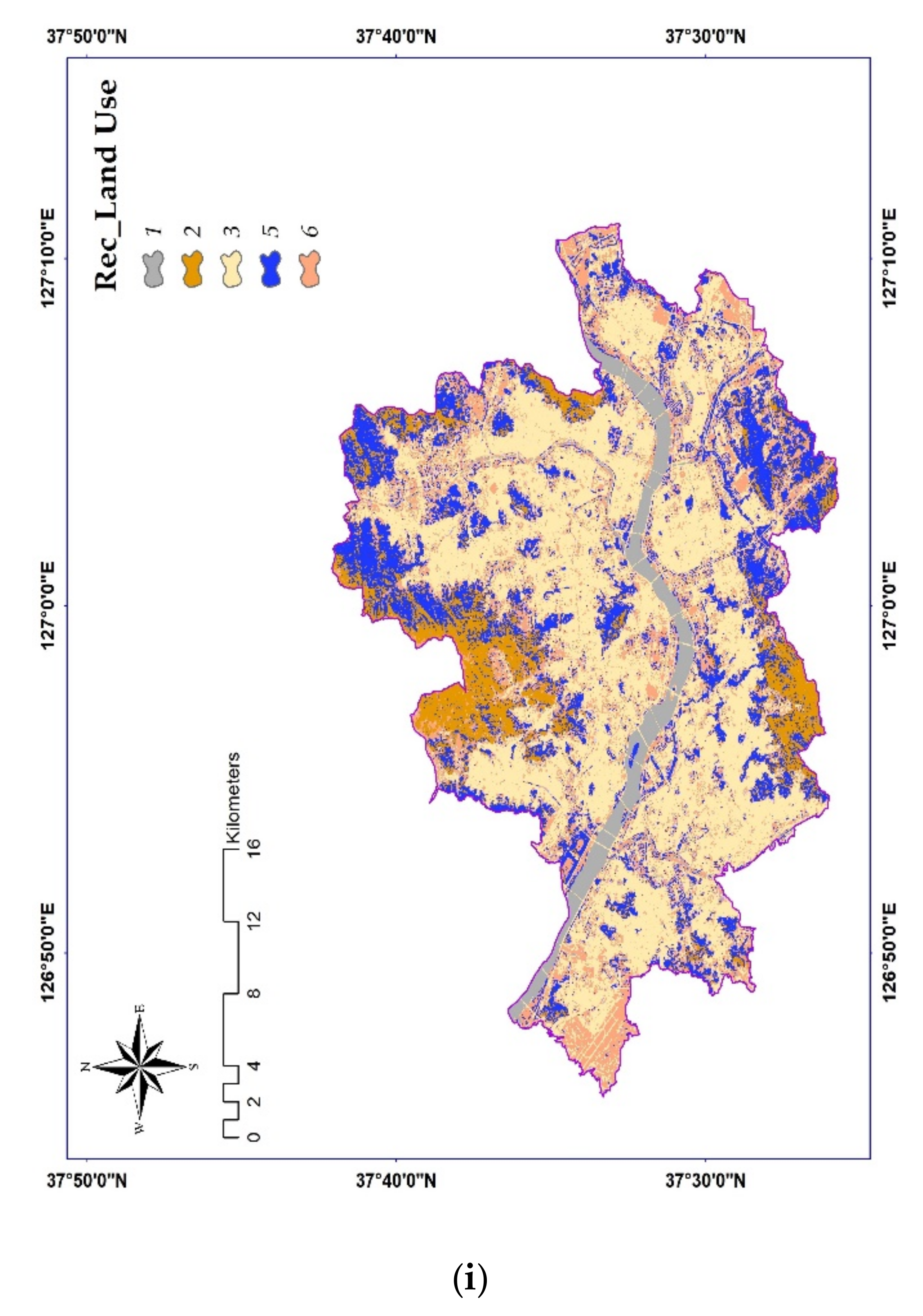
This factor is calculated by dividing the total length of all streams in a drainage basin by the drainage basin’s total area [35] using spatial analyst tools in ArcGIS. The stream layer extracted from the DEM is the basic map to prepare a drainage map. According to Das and Pardeshi [36], a high drainage density indicates considerable surface runoff and low-groundwater-potential zone. In this study, the drainage density varied from 0.77 to 3.14 km/km², as shown in Figure 3h, and was classified into the following four classes: <0.78, 0.78–1.57, 1.57–2.36, and >3.14 km/km².

2.3.9. Land Use

According to Yalcin [37], this factor is crucial in determining several hydrological processes, such as the rate of soil infiltration, evapotranspiration, and surface runoff. As mentioned before, Landsat 8 images with the lowest percentage of cloud cover were obtained from the United States Geological Survey official website, and the ArcGIS and Erdas Imagine were used to process satellite imageries for land use change assessment of this study area. In order to derive supervised land use classification, maximum likelihood classification algorithm was used in this study. The pixel color tone for each land use class was identified using ArcGIS and verified using google earth. For the final stage, Erdas Imagine was used for accuracy assessment of supervised land use classification. As Figure 3i shows, the major land uses in the study area are: (i) urban areas, (ii) several types of vegetation, (iii) water bodies, (iv) forests, and (v) bare land with a kappa accuracy of 0.92.

2.4. AHP

After preparing all nine layers, including DEM, mean rainfall, land use, slope, distance from river, flow accumulation, TWI, drainage density, and plan curvature (Figure 3), the AHP model was used to assign different weights to each thematic layer. AHP is the MCDM method implemented by ArcGIS, which was developed by Saaty [38], and this approach involves determining the weights and ranks of different flooding parameters. The total weight of each map of the final integrated layer is computed as

$$\begin{array}{c}\mathrm{FH}=\left({\mathrm{E}}_{\mathrm{w}}·{\mathrm{E}}_{\mathrm{r}}\right)+\left({\mathrm{S}}_{\mathrm{w}}·{\mathrm{S}}_{\mathrm{r}}\right)+\left({\mathrm{D}}_{\mathrm{w}}·{\mathrm{D}}_{\mathrm{r}}\right)+\left({\mathrm{R}}_{\mathrm{w}}·{\mathrm{R}}_{\mathrm{r}}\right)+\left({\mathrm{F}}_{\mathrm{w}}·{\mathrm{F}}_{\mathrm{r}}\right)+\left({\mathrm{T}}_{\mathrm{w}}·{\mathrm{T}}_{\mathrm{r}}\right)+\left({\mathrm{C}}_{\mathrm{w}}·{\mathrm{C}}_{\mathrm{r}}\right)\\ +\left({\mathrm{DR}}_{\mathrm{w}}·{\mathrm{DR}}_{\mathrm{r}}\right)+\left({\mathrm{L}}_{\mathrm{w}}·{\mathrm{L}}_{\mathrm{r}}\right)\end{array}$$

(2)

where FH is the flood hazard index, w represents the weight of each criterion, and r is the rating of each criterion with the following names: DEM (E), mean rainfall (R), land use (L), slope (S), distance from river (D), flow accumulation (F), TWI (T), drainage density (DR), and plan curvature (C).

The FH model was used to assess the vulnerability of flood incidence, and finally, the flood map was categorized into six regions using the weights of each sub-criterion in ArcGIS: very high risk, high risk, medium risk, low risk, very low risk, and out of risk. In this study, pairwise comparison matrices were developed using the AHP extension in the ArcGIS, which involved all nine criteria to determine which of them has higher priority. In this regard, Saaty [38] suggested a scale of 1 to 9 for each criterion compared to the other elements (

Table 1. Pairwise comparison scale for AHP [38].

Numerical Rating	Definition
1	Equal importance in a pair
3	Moderate importance
5	Strong importance
7	Very strong importance
9	Extreme importance
2, 4, 6, 8	Intermediate values

). After weighting all elements, the values in the pairwise comparison are normalized and the average random consistency indices (

Table 2. Average random consistency indices (RIs) for different number of criteria (N), adapted from [39].

N	1	2	3	4	5	6	7	8	9	10	11	12	13	14	15
RI	0	0.0	0.58	0.90	1.12	1.24	1.32	1.41	1.45	1.49	1.51	1.54	1.56	1.57	1.59

) according to the number of criteria (here, the number of criteria is nine) are chosen to express the consistency ratio with the following equation:

$$\mathrm{CR}=\frac{\mathrm{CI}}{\mathrm{RI}}$$

(3)

$$\mathrm{CI}=\frac{\mathsf{\lambda }\max -\mathrm{n}}{\mathrm{n}-1}$$

(4)

where CR is the consistency ratio, CI represents the consistency index, RI is the random consistency index, $\mathsf{\lambda }\max$ represents the principal eigenvalue of the matrix, and n is the number of components or criteria in the matrix.

2.5. Nine Controlling Factors with Their Relative Weights

In this study, nine thematic layers were considered for flood susceptibility mapping and their weights were determined from the AHP model using pairwise comparison matrix. It should be noted that, the novelty of this study lies in the preparation of maps from satellite images without direct intervention. Thus, all nine maps were extracted, using collected DEM from satellite images, to prepare the flood susceptibility map. The details of the pairwise comparison matrix is listed in

Table 3. Pairwise comparison matrix of expert opinions with CI and CR (here, E: DEM, S: slope, D: Distance from river, R: mean rainfall, F: flow accumulation, T: TWI, C: plan curvature, DR: drainage density, L: land use, W: weights, CI: consistency index, CR: consistency ratio).

Parameters	E	S	D	R	F	T	C	DR	L	W	CI	CR
E	1	2	2	2	5	6	5	3	4	0.24	0.14	0.1
S	0.5	1	2	3	4	4	4	2	5	0.2	0.14	0.1
D	0.5	0.5	1	0.5	3	4	5	2	3	0.13	0.14	0.1
R	0.5	0.33	2	1	2	3	5	2	4	0.14	0.14	0.1
F	0.2	0.25	0.3	0.5	1	3	4	0.5	2	0.07	0.14	0.1
T	0.17	0.25	0.3	0.33	0.33	1	3	3	0.3	0.06	0.14	0.1
C	0.2	0.25	0.2	0.2	0.25	0.33	1	0.25	0.5	0.03	0.14	0.1
DR	0.33	0.5	0.5	0.5	2	0.33	4	1	0.3	0.07	0.14	0.1
L	0.25	0.2	0.3	0.25	0.5	3	2	3	1	0.07	0.14	0.1

. According to Saaty [38], the CR is acceptable if the value is <0.10, which indicates a reasonable level for the pairwise comparison matrix. In the ArcGIS program, when the sentence “The matrix is considered consistent enough” is displayed, it means that the result is accepted. Subsequently, all parameters are assessed individually and are classified into different subcategories.

Table 4. Pairwise comparison matrix for sub-criteria of the nine parameters with their weights.

Sb. No.	Elements	Pairwise Comparison Matrix					CR	Weight
1	DEM
	<75	1	3	5	7	8	0.588	0.499
	75–145	0.33	1	3	5	6		0.255
	145–249	0.2	0.33	1	3	5		0.137
	249–395	0.14	0.2	0.33	1	3		0.069
	>395	0.12	0.16	0.2	0.33	1		0.037
2	Slope
	>70	1	2	3	5	7	0.035	0.446
	17–26	0.5	1	3	5	7		0.297
	10–17	0.25	0.33	1	3	5		0.146
	4–10	0.16	0.2	0.33	1	3		0.072
	<4	0.12	0.14	0.2	0.33	1		0.036
3	Distance from River
	<50	1	2	4	6	8	0.018	0.464
	50–100	0.5	1	2	4	6		0.264
	100–200	0.25	0.5	1	2	5		0149
	200–400	0.16	025	0.5	1	3		0.082
	>500	0.12	0.16	0.2	0.33	1		0.038
4	Mean Rainfall
	>22	1	3	5	7	9	0.056	0.491
	15–18	0.33	1	3	7	9		0.286
	9–15	0.2	0.33	1	3	5		0.127
	4–9	0.14	0.14	0.33	1	3		0.061
	<4	0.11	0.11	0.2	0.33	1		0.032
5	Flow Accumulation
	>1,074,483	1	2	4	6	8	0.028	0.461
	720,132–1,074,483	0.5	1	2	4	6		0.262
	285,766–720,132	0.25	0.5	1	2	5		0.148
	57,153–285,766	0.16	0.25	0.5	1	4		0.089
	<57,153	0.12	0.16	0.2	0.25	1		0.037
6	TWI
	>24	1	3	5	7	9	0.050	0.503
	10–13	0.33	1	3	5	7		0.260
	8–10	0.2	0.33	1	3	5		0.134
	6–8	0.14	0.2	0.33	1	3		0.067
	<6	0.11	0.14	0.2	0.33	1		0.034
7	Plan Curvature
	<−1.10	1	3	5	7	9	0.050	0.503
	−1.10 to −0.38	0.33	1	3	5	7		0.260
	−0.38 to 0.24	0.2	0.33	1	3	5		0.134
	0.2–0.8	0.14	0.2	0.33	1	3		0.067
	>17	0.11	0.14	0.2	0.33	1		0.034
8	Drainage Density
	<0.30	1	3	5	7	9	0.018	0.518
	0.30–0.69	0.33	1	3	5	6		0.262
	0.69–1.09	0.2	0.33	1	2	3		0.111
	1.09–1.58	014	0.2	0.5	1	2		0.066
	>3.14	011	0.16	0.33	0.5	1		0.041
9	Land Use
	Water Bodies	1	2	3	5	6	0.016	0.419
	Bare Land	0.5	1	2	6	5		0.292
	Urban Area	0.33	0.5	1	3	4		0.170
	Forest	0.2	0.16	0.33	1	1		0.060
	Vegetation	0.16	0.2	0.25	1	1		0.056

shows the different ranks for each sub-category using the AHP extension in the ArcGIS program.

According to experts’ opinion, elevation plays the most effective role in flood mapping [40,41], and thus receives the highest weight in the method developed by Saaty [38], as shown in Table 3. This means that regions located at higher elevations have lower potential to be flooded and vice versa for lower-altitude areas. Thus, the highest altitudes receive the lowest weight, as shown in Table 4. According to the study conducted by Das and Pardeshi [36] on hydrology, slope also plays a crucial role in directing water to downstream areas and is an important factor after elevation. Regarding this issue, as the slope increases, the flow rate also increases, and the infiltration process is reduced. Thus, high amounts of water flowing in streams often leads to flooding. Distance from the river, as a geomorphic factor, is another important factor in flood occurrence. Regions far from the river have lower vulnerability to flood occurrence. The drainage network and flow accumulation had almost the same weight. Flow accumulation refers to the concentration of flow and is directly related to flood occurrence [42]. Meanwhile, a higher density of drainage network simplifies the draining runoff, and thus reduces the risk of flooding.

Land use of area is the type of natural and man-made land. In this study, the following five categories of land use were adopted: water bodies, urban areas, bare land, forest, and vegetation. Some activities such as deforestation and urbanization have serious effects on flood occurrence. In highly built-up regions, flood situations occur frequently due to an increase in population. As shown in Figure 3i, the urban area in red has the largest area and exhibits the highest effect on flood occurrence. TWI represents the effect of topography on runoff generation and flow accumulation in river catchments [41]. It has a direct effect on flood occurrences, which means that regions with higher TWI have a higher vulnerability to flooding. Among the nine factors, plan curvature has a minor effect on floods, which cannot be neglected. In this study, the following three shapes were considered: concave, flat, and convex. Negative values represent concave shapes, positive values show convex shapes, and near-zero indicates flat areas. In the heightening curvature map, the negative value has the highest weight because it plays a more important role in flood occurrence. Rainfall, as the final layer, plays a significant role and has a direct relation with the Han River discharge; thus, it can control the flood occurrence.

After determining weights for each of the criteria and sub-criteria, the AHP extension in ArcGIS was used to find the optimum CR for the highest accuracy. When the statement “The matrix is regarded to be consistent enough” appears in the produced table, it implies that the result has been accepted and this weight is suitable for use in reclassification and overlay operations. In reclassification, all criteria were divided into five sub-criteria by considering the weights developed in AHP.

3. Results and Discussion

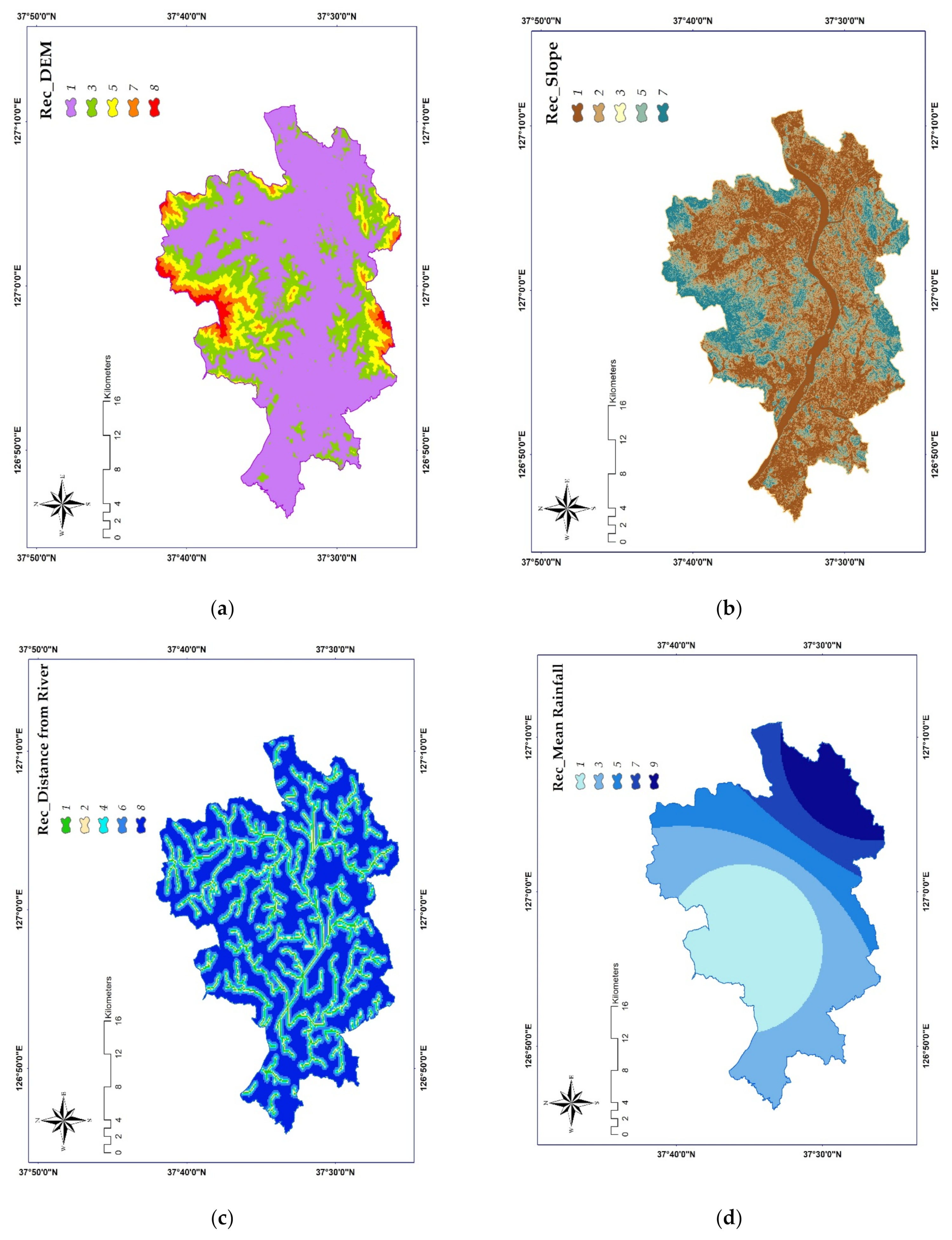
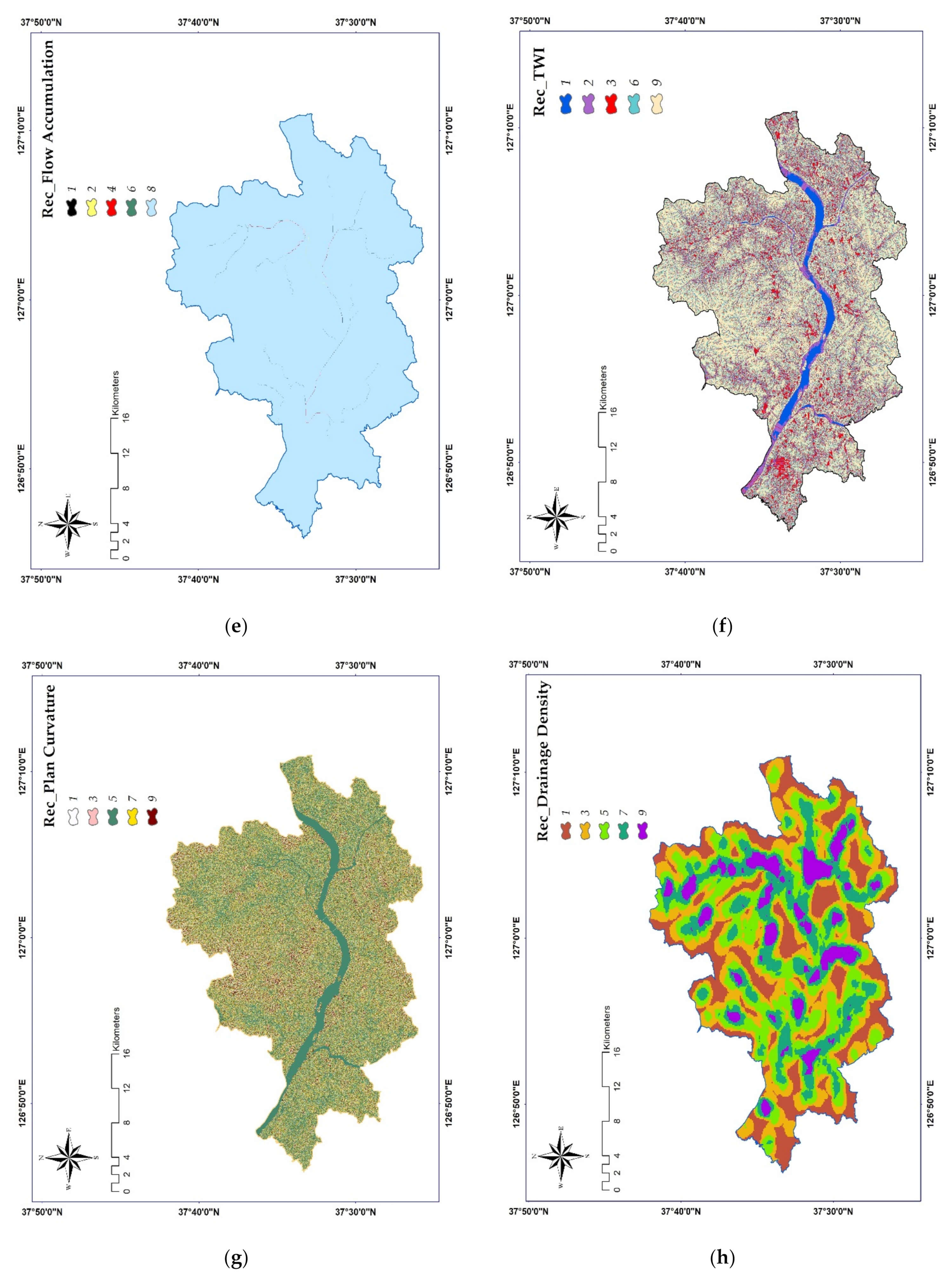
3.1. Reclassification for Each Thematic Layer

In this study, nine criteria were converted into the raster format to identify flood sensitive areas. AHP was applied for the weighting, ranking, and reclassifying of these maps in ArcGIS. These criteria can provide a flood hazard location in a specific region when combined with the AHP technique. According to Saaty [38], a pairwise comparison matrix and the amount of CI and CR were established using ArcGIS. The results showed that CR is acceptable because it has a value of less than 0.10. This demonstrates that pairwise comparison has a sensible consistency dimension. After obtaining this reasonable result, all parameters were assessed individually and classified into five subcategories using ArcGIS; for instance, high-elevation areas have a lower risk of flooding, whereas low-altitude areas have a higher risk. Thus, higher elevations have a high value, whereas lower elevations have a low value (Figure 4a). The classification was repeated for all thematic layers, based on their effects on floods and their detailed information was summarized in Figure 4. To be more descriptive, ratings were provided to classes in each thematic layer based on its relative importance for flood susceptibility, and all thematic layers were reclassified to five different categories regarding to the Table 4. According to all nine reclassified thematic layers (Figure 4), central part to the western regions are more vulnerable to flood than the northern and southern regions because of low elevation (purple color with rank 1 in Figure 4a), low slope (dark brown color with rank 1 in Figure 4b), and high amount of rainfall (light blue color with rank 1 in Figure 4d).

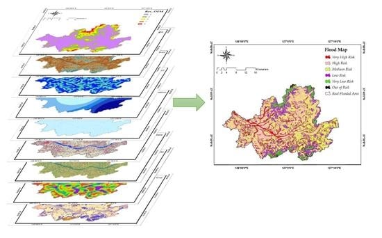
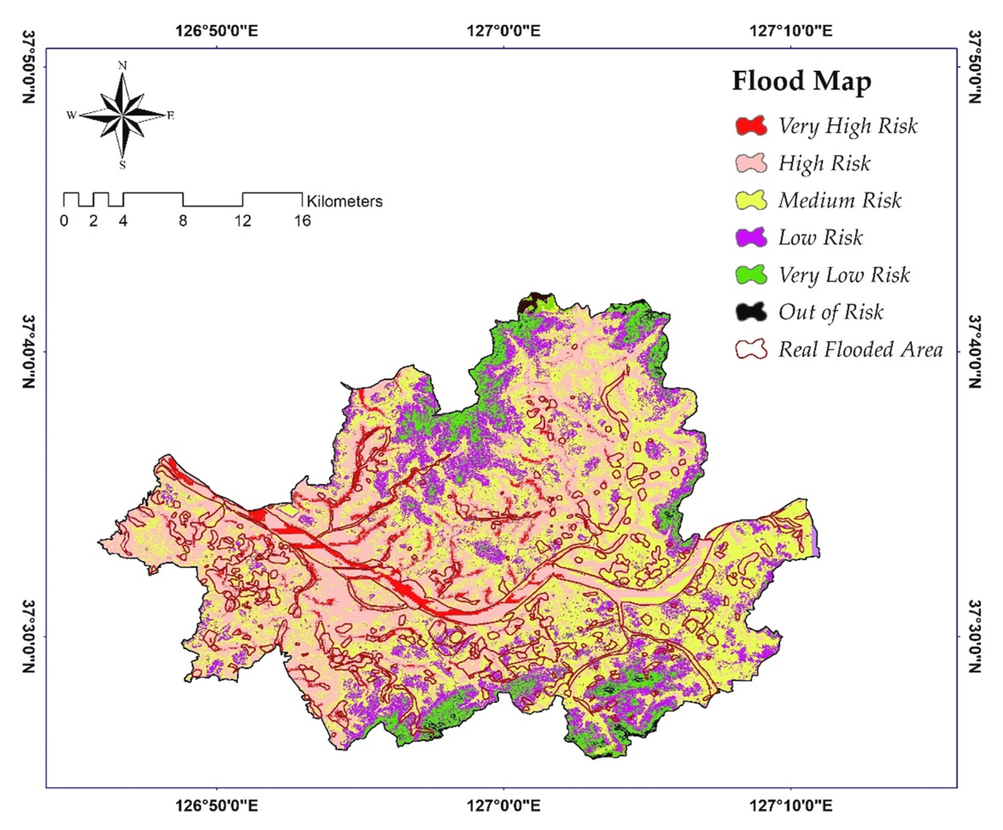
3.2. Flood Susceptibility Map

In Table 4, the weight of the relevant factors and their relationships with flood occurrence are shown for each thematic layer. Based on the values in this table, among the different land use types, water bodies, bare land, and urban area had the highest weights, which indicated a positive influence on flooding, whereas forest area had a positive influence on decreasing floods, and thus its corresponding weight was lesser than that of the other categories. In the case of the rainfall map, the area with a high amount of rain has a higher weight, and this value decreases for areas with low levels of rainfall. This classification is the same for slope, TWI, and flow accumulation. However, in the case of DEM, distance from the river, drainage network, and plan curvature, the weighting is the opposite; thus, areas with higher values receive lower weights. Based on this relation, after reclassification for each criterion, the flood susceptibility map was extracted and categorized into the following six regions using the natural breaking method in ArcGIS (Figure 5): very high risk, high risk, medium risk, low risk, very low risk, and out of risk.

For example, the area with the level of very high risk has the highest elevation, slope, rainfall, TWI and flow accumulation, as well as the lowest distance from river and lowest drainage network. Moreover, the very high risk areas have a negative value for plan curvature and located in urban area and bare lands. Figure 5 shows that the high-flood-potential location is to the western area of Seoul, near the Han River. To better understand this type of flood susceptibility map, it is reasonable to refer to the previous basic maps (Figure 3) because these maps are directly relevant to the final map. DEM and slope play crucial roles in flood occurrence. As shown in Figure 3, the green areas have the lowest slope and are situated in the central portion of the basin, which is approximately 28%. In addition, the central part of Seoul from east to west shows the lowest amount of elevation, which is indicated in dark pink in Figure 3a. That is, elevation and slope can contribute to make the Han River overflow, along with monsoon rainfall in the region. In the study area, the roles of forests and vegetation would be ignored in the central part of Seoul because this location is replaced with urban areas and there are no natural places, except for some parks and man-made areas. Zaharia [43] indicated that places with slopes exceeding 15° do not favor water accumulation, whereas those with a large cover of forest and dense vegetation and a flat surface favors the retention of excess surface water during a flood.

The results revealed that the area was categorized into the following six flood potential zones: very high risk (4%), high risk (36%), medium risk (37%), low risk (16%), very low risk (6%), and out of risk (1%). The area with a very high risk level is concentrated in the central-western part of Seoul, which is characterized by a low elevation and low slope, with high levels of rainfall. Moreover, the small part of the northern and southern parts of Seoul either exhibit very low risk or are out of risk, as the elevation is very high, and the slope exceeds 40°. This area, with a dense cover of forest and vegetation, is at risk of flood occurrence.

The flood susceptibility map was validated from comparison results with a real flood map (Figure A1) obtained from Seoul Metropolitan government for the years of 2001, 2010, 2011, 2012, and 2013. At this point, the total flooded areas (Figure A1) were merged into Figure 5 and the number of pixels associated with each polygon was counted to evaluate the accuracy and validation of the model.

Table 5. Number of counted pixels in six different categories of flooded area.

Regions	Number of Pixel	Percentage
Very High Risk	63,613	9.94%
High Risk	344,668	53.87%
Medium Risk	197,236	30.83%
Low Risk	31,982	5%
Very Low Risk	2289	0.36%
Out of Risk	50	0.01%

and Figure 6 describe the number of cells assigned to each of the six categories and the number of corresponding pixels according to the flood susceptibility map with resolution of 12.5 m in Figure 5, which was extracted using spatial analyst toolbar in ArcGIS for validation purposes. According to Table 5, in total, 94.64% of areas are located in the very high risk, high risk and medium risk regions, and 5.37% is located in low risk, very low risk, and out of risk regions. It means that the proposed method can be useful in identifying flood-prone areas with a priority for mitigation and adaptation approaches for water resources management.

On the other hand, the comparison indicates that the flood susceptibility map obtained from this study is consistent with a real flood hazard and that the western part of Seoul has more potential for flooding (Figure 5). The accuracy of the AHP technique depends on the assigned weights, which vary for each topic. For instance, elevation [44] and slope [45] as the most important factors in the topic of flood prone areas receive the highest weights. These results indicate that flooding occurs most often along riverbanks and only occasionally in areas far from rivers.

3.3. Further Discussion

In flood susceptibility analysis, the major aim is to find areas that may be affected by floods in the future. Thus, it is irrelevant which integration method is used (e.g., AHP as a simple method or AI as a complex method), but the validation of this flood susceptibility map is the most important in terms of determining the unknown future flood events [46]. As the first step, creating high-resolution basic maps helps increase the accuracy of the final map; thus, choosing satellite images of the case study area of Seoul with the lowest cloud cover would be effective in determining flood-prone areas. The use of a real flood map is the second step for validation, which helps decision-makers and administrative bodies improve the accuracy of flood-mapping in management and planning by comparing the mapping results with those obtained using real maps. In Figure 5, the locations that are very high risk and high risk are colored in red and pink, respectively; however, even though moderately sensitive regions are categorized in the third classification, they should not be ignored in terms of high priority for flood management. On the other hand, regarding to the Figure 3i, the vegetation cover has decreased compared to other previous years (not included in this study), which could be one of the factors associated with increasing floods. Thus, the pink and red areas need serious attention from administrative bodies to prevent flood situations in the near future.

The major challenge of this study is the opinion of experts and Saaty’s [38] method for preparing the appropriate weights of each parameter in extracting the flood map, because factors such as expert tiredness, lack of sufficient expertise, and lack of appropriate measuring devices greatly influence the weighting of the controlling variables. However, a soil texture map [47] and a geology map [48] were not considered for flood susceptibility mapping because of inaccurate satellite images obtained for the year of 2020, but the new land use map was extracted for the year of 2020 to specify the percentage of increasing the urban areas. At the final stage, the results for the year of 2020 were compared with a map that belongs to the years of 2001, 2010, 2011, 2012, and 2013 (Figure A1). As it has been shown, little difference was found between the two maps because this study extracted new maps to divide areas in terms of flood susceptibility.

Flood susceptibility mapping through the AHP model is expected to be used in management studies related to risk assessment and mitigation strategies for flooding, as it determines the most vulnerable areas based on physical characteristics that influence flooding risk. Overall, future research will focus on issues related to data consolidation, such as resolution, generalization, and integration. Furthermore, the AHP methodology will be compared to other approaches for evaluating flood susceptibility, in order to determine the best alternative, including more robust validation with data collection.

4. Conclusions

Floods are the most destructive natural disasters worldwide. Therefore, to achieve sustainable growth, flood susceptibility mapping is required for integrated watershed management. In this study, flood prone areas were identified by integrating the AHP method and geospatial techniques, and for validating the results, a flood inventory map containing flood regions was obtained from the Seoul Metropolitan government [49]. First, nine thematic layers, due to the most effective role in the occurrence of floods, were derived using satellite images and ArcGIS. Then, a flood susceptibility map was extracted using appropriate weights and CR. Approximately 40% of the total area was found to belong to the very high risk and high risk zones, which are located in the western and central parts of Seoul, near the Han River, with a flat slope and low elevation. It is noted that the methodology presented in this study can be a useful and easier approach for creating a flood susceptibility map.

Satellite images were used to detect flood hazard-zones. In particular, Landsat 8 was used to extract a new map of land use/landscape in 2020. Previous studies only used the old version of the land use map and considered the basic maps that were extracted in different years. Therefore, using all maps from a particular year (i.e., 2020 in this study) can be effective to obtain suitable results; this was the focus of this study. For instance, in the case study of Seoul, the growth of urban areas is a significant factor in the preparation of land use maps, and it should not be ignored for countries like Korea. Furthermore, a DEM was obtained from the ALOS PALSAR sensor with a high resolution of 12.5 m, which is an advantage of the presented method because this map helps extract the seven basic maps including elevation, slope, flow accumulation, TWI, drainage network, plan curvature, and distance from the river with high resolution for additional use in subsequent map development and analysis. Another novelty of this study is the use of basic maps without human intervention, which are appropriate for ungauged areas. In addition, each map was reclassified into five categories to determine the direct impact of each part on the flood-prone area, which is another advantage of the proposed method. Finally, the number of pixels related to each polygon extracted from the real flood map was counted to assess the accuracy and validation of the flood susceptibility map obtained from this study. The results indicate that the proposed method shows the high performance of identifying the flood prone area. The region was classified into six classes in terms of flood susceptibility by integration of ArcGIS and the study area.

This study is a new approach for obtaining flood susceptibility map, which focused on: (1) preparation of basic maps with high resolution of satellite images; (2) extraction of a new land use map for the year of 2020 to clarify the growth in urban area with all updated maps for the same year of 2020 without direct human intervention; (3) validation of the extracted flood susceptibility map with the real flood map by counting the number of pixels in flooded areas. Therefore, it should be noted that the proposed method just considers satellite images, ArcGIS, and AHP for obtaining a flood susceptibility map, which can be used in any other geographical area with available satellite images. It can help decision-makers and planners to perform suitable flood management in the future, especially in the identification and analysis stages of risk assessment projects.

References

1. Padli, J.; Habibullah, M.S.; Baharom, A.H. Determinants of Flood Fatalities: Evidence from a Panel Data of 79 Countries. Soc. Sci. Humanit. 2013, 21, 81–98. [Google Scholar]
2. Pourghasemi, H.R.; Jirandeh, A.G.; Pradhan, B.; Xu, C.; Gokceoglu, C. Landslide Susceptibility Mapping Using Support Vector Machine and GIS at the Golestan Province, Iran. J. Earth Syst. Sci. 2013, 122, 349–369. [Google Scholar] [CrossRef] [Green Version]
3. Mishra, K.; Sinha, R. Flood Risk Assessment in the Kosi Megafan Using Multi-Criteria Decision Analysis: A Hydro-Geomorphic Approach. Geomorphology 2020, 350, 106861. [Google Scholar] [CrossRef]
4. Das, S. Flood Susceptibility Mapping of the Western Ghat Coastal Belt Using Multi-Source Geospatial Data and Analytical Hierarchy Process (AHP). Remote Sens. Appl. Soc. Environ. 2020, 20, 100379. [Google Scholar] [CrossRef]
5. Sampson, C.C.; Smith, A.M.; Bates, P.D.; Neal, J.C.; Alfieri, L.; Freer, J.E. A High-Resolution Global Flood Hazard Model. Water Resour. Res. 2015, 51, 7358–7381. [Google Scholar] [CrossRef] [PubMed] [Green Version]
6. MohanRajan, S.N.; Loganathan, A.; Manoharan, P. Survey on Land Use/Land Cover (LU/LC) Change Analysis in Remote Sensing and GIS Environment: Techniques and Challenges. Environ. Sci. Pollut. Res. Int. 2020, 27, 29900–29926. [Google Scholar] [CrossRef] [PubMed]
7. De Brito, M.M.; Evers, M.; Almoradie, A.D.S. Participatory Flood Vulnerability Assessment: A Multi-Criteria Approach. Hydrol. Earth Syst. Sci. 2018, 22, 373–390. [Google Scholar] [CrossRef] [Green Version]
8. Lee, M.J.; Kang, J.E.; Kim, G. Application of Fuzzy Combination Operators to Flood Vulnerability Assessments in Seoul, Korea. Geocarto Int. 2015, 30, 1–24. [Google Scholar] [CrossRef]
9. Nourani, V.; Tahershamsi, A.; Abbaszadeh, P.; Shahrabi, J.; Hadavandi, E. A New Hybrid Algorithm for Rainfall-Runoff Process Modeling Based on the Wavelet Transform and Genetic Fuzzy System. J. Hydroinf. 2014, 16, 1004–1024. [Google Scholar] [CrossRef] [Green Version]
10. Danandeh Mehr, A.; Kahya, E.; Olyaie, E. Streamflow Prediction Using Linear Genetic Programming in Comparison with a Neurowavelet Technique. J. Hydrol. 2013, 505, 240–249. [Google Scholar] [CrossRef]
11. Guo, E.; Zhang, J.; Ren, X.; Zhang, Q.; Sun, Z. Integrated Risk Assessment of Flood Disaster Based on Improved Set Pair Analysis and the Variable Fuzzy Set Theory in Central Liaoning Province China. Nat. Hazards 2014, 74, 947–965. [Google Scholar] [CrossRef]
12. Tehrany, M.S.; Pradhan, B.; Jebur, M.N. Spatial Prediction of Flood Susceptible Areas Using Rule-Based Decision Tree (DT) and a Novel Ensemble Bivariate and Multivariate Statistical Models in GIS. J. Hydrol. 2013, 504, 69–79. [Google Scholar] [CrossRef]
13. Darabi, H.; Choubin, B.; Rahmati, O.; Torabi Haghighi, A.T.; Pradhan, B.; Kløve, B. Urban Flood Risk Mapping Using the GARP and QUEST Models: A Comparative Study of Machine Learning Techniques. J. Hydrol. 2019, 569, 142–154. [Google Scholar] [CrossRef]
14. Souissi, D.; Msaddek, M.H.; Zouhri, L.; Chenini, I.; El May, M.; Dlala, M. Mapping Groundwater Recharge Potential Zones in Arid Region Using GIS and Landsat Approaches, Southeast Tunisia. Hydrol. Sci. J. 2018, 63, 251–268. [Google Scholar] [CrossRef]
15. Hwang, C.L.; Yoon, K. Methods for Multiple Attribute Decision Making. In Lecture Notes in Economics and Mathematical Systems; Springer: Berlin/Heidelberg, Germany, 1981; pp. 58–191. [Google Scholar] [CrossRef]
16. Al-Harbi, K.M.A. Application of the AHP in Project Management. Int. J. Proj. Manag. 2001, 19, 19–27. [Google Scholar] [CrossRef]
17. Allafta, H.; Opp, C.; Patra, S. Identification of Groundwater Potential Zones Using Remote Sensing and GIS Techniques: A Case Study of the Shatt Al-Arab Basin. Remote Sens. 2021, 13, 112. [Google Scholar] [CrossRef]
18. Wang, H.B.; Wu, S.R.; Shi, J.S.; Li, B. Qualitative Hazard and Risk Assessment of Landslides: A Practical Framework for a Case Study in China. Nat. Hazards 2013, 69, 1281–1294. [Google Scholar] [CrossRef]
19. Ajay Kumar, V.A.; Mondal, N.C.; Ahmed, S. Identification of Groundwater Potential Zones Using RS, GIS and AHP Techniques: A Case Study in a Part of Deccan Volcanic Province (DVP), Maharashtra, India. J. Indian Soc. Remote Sens. 2020, 48, 497–511. [Google Scholar] [CrossRef]
20. Shao, Z.; Huq, M.E.; Cai, B.; Altan, O.; Li, Y. Integrated Remote Sensing and GIS Approach Using Fuzzy-AHP to Delineate and Identify Groundwater Potential Zones in Semi-Arid Shanxi Province, China. Environ. Modell. Softw. 2020, 134, 104868. [Google Scholar] [CrossRef]
21. Chen, Y.R.; Yeh, C.H.; Yu, B. Integrated Application of the Analytic Hierarchy Process and the Geographic Information System for Flood Risk Assessment and Flood Plain Management in Taiwan. Nat. Hazards 2011, 59, 1261–1276. [Google Scholar] [CrossRef] [Green Version]
22. Sinha, R.; Bapalu, G.V.; Singh, L.K.; Rath, B. Flood Risk Analysis in the Kosi River Basin, North Bihar Using Multi-Parametric Approach of Analytical Hierarchy Process (AHP). J. Indian Soc. Remote Sens. 2008, 36, 335–349. [Google Scholar] [CrossRef]
23. Zangemeister, C. Nutzwertanalyse in der Systemtechnik; Wittemannsche Buchhandlung: Winnemark, Germany, 1971; Available online: www.zangemeister.de (accessed on 20 April 2021).
24. Kazibudzki, P.T. The Quality of Ranking During Simulated Pairwise Judgments for Examined Approximation Procedures. Model. Simul. Eng. 2019, 2019, 13. [Google Scholar] [CrossRef] [Green Version]
25. Stefanidis, S.; Stathis, D. Assessment of Flood Hazard Based on Natural and Anthropogenic Factors Using Analytic Hierarchy Process (AHP). Nat. Hazards 2013, 68, 569–585. [Google Scholar] [CrossRef]
26. Grozavu, A.; Pleşcan, S.; Mărgărint, C. Comparative Methods for the Evaluation of the Natural Risk Factors Importance. Present Environ. Sustain. Dev. 2011, 5, 33–40. [Google Scholar]
27. Statistical of Seoul, Seoul Metropolitan Government. 2016. Available online: http://data.seoul.go.kr/ (accessed on 20 April 2021).
28. Lee, S.; Kim, J.C.; Jung, H.S.; Lee, M.J.; Lee, S. Spatial Prediction of Flood Susceptibility Using Random-Forest and Boosted-Tree Models in Seoul Metropolitan City, Korea. Geom. Nat. Hazards Risk 2017, 8, 1185–1203. [Google Scholar] [CrossRef] [Green Version]
29. Shin, J.I. Historic River Flowing Through the Korean Peninsula. Koreana 2004, 6, 4–11. [Google Scholar]
30. Date, I. Britannica, the Editors of Encyclopaedia. Han River. Encyclopedia Britannica. Available online: https://www.britannica.com/place/Han-River-South-Korea (accessed on 20 April 2021).
31. Lee, Y.; Brody, S.D. Examining the Impact of Land Use on Flood Losses in Seoul, Korea. Land Use Policy 2018, 70, 500–509. [Google Scholar] [CrossRef]
32. Zhou, Q.; Pilesjö, P.; Chen, Y. Estimating Surface Flow Paths on a Digital Elevation Model Using a Triangular Facet Network. Water Resour. Res. 2011, 47. [Google Scholar] [CrossRef]
33. Grabs, T.; Seibert, J.; Bishop, K.; Laudon, H. Modeling Spatial Patterns of Saturated Areas: A Comparison of the Topographic Wetness Index and a Dynamic Distributed Model. J. Hydrol. 2009, 373, 15–23. [Google Scholar] [CrossRef] [Green Version]
34. Tehrany, M.S.; Pradhan, B.; Jebur, M.N. Flood Susceptibility Mapping Using a Novel Ensemble Weights-of-Evidence and Support Vector Machine Models in GIS. J. Hydrol. 2014, 512, 332–343. [Google Scholar] [CrossRef]
35. Harini, P.; Sahadevan, D.K.; Das, I.C.; Manikyamba, C.; Durgaprasad, M.; Nandan, M.J. Regional Groundwater Assessment of Krishna River Basin Using Integrated GIS Approach. J. Indian Soc. Remote Sens. 2018, 46, 1365–1377. [Google Scholar] [CrossRef]
36. Das, S.; Pardeshi, S.D. Integration of Different Influencing Factors in GIS to Delineate Groundwater Potential Areas Using IF and FR Techniques: A Study of Pravara Basin, Maharashtra, India. Appl. Water Sci. 2018, 8, 1–16. [Google Scholar] [CrossRef] [Green Version]
37. Yalcin, A.; Reis, S.; Aydinoglu, A.C.; Yomralioglu, T. A GIS-Based Comparative Study of Frequency Ratio, Analytical Hierarchy Process, Bivariate Statistics and Logistics Regression Methods for Landslide Susceptibility Mapping in Trabzon, NE Turkey. CATENA 2011, 85, 274–287. [Google Scholar] [CrossRef]
38. Saaty, T.L. The Analytic Hierarchy Process: Planning, Priority Setting, Resource Allocation; McGraw-Hill Inc.: New York, NY, USA, 1980. [Google Scholar]
39. Saaty, T.L. Decision Making for Leaders: The Analytic Hierarchy Process for Decisions in a Complex World; RWS Publications: Pittsburgh, PA, USA, 1990. [Google Scholar]
40. Botzen, W.J.W.; Aerts, J.C.J.H.; Van den Bergh, J.C.J.M. Individual Preferences for Reducing Flood Risk to near Zero Through Elevation. Mitig. Adapt. Strateg. Glob. Chang. 2013, 18, 229–244. [Google Scholar] [CrossRef] [Green Version]
41. Mojaddadi, H.; Pradhan, B.; Nampak, H.; Ahmad, N.; Ghazali, A.H. Ensemble Machine-Learning-Based Geospatial Approach for Flood Risk Assessment Using Multi-Sensor Remote-Sensing Data and GIS. Geom. Nat. Hazards Risk. 2017, 8, 1080–1102. [Google Scholar] [CrossRef] [Green Version]
42. Tehrany, M.S.; Pradhan, B.; Mansor, S.; Ahmad, N. Flood Susceptibility Assessment Using GIS-Based Support Vector Machine Model with Different Kernel Types. CATENA 2015, 125, 91–101. [Google Scholar] [CrossRef]
43. Zaharia, L.; Costache, R.; Prăvălie, R.; Ioana-Toroimac, G. Mapping Flood and Flooding Potential Indices: A Methodological Approach to Identifying Areas Susceptible to Flood and Flooding Risk. Case Study: The Prahova Catchment (Romania). Front. Earth Sci. 2017, 11, 229–247. [Google Scholar] [CrossRef]
44. Mohammadi, M.; Darabi, H.; Mirchooli, F.; Bakhshaee, A.; Haghighi, A.T. Flood Risk Mapping and Crop-Water Loss Modeling Using Water Footprint Analysis in Agricultural Watershed, Northern Iran. Nat. Hazards 2020, 105, 2007–2025. [Google Scholar] [CrossRef]
45. Rahmati, O.; Zeinivand, H.; Besharat, M. Flood Hazard Zoning in Yasooj Region, Iran, Using GIS and Multi-Criteria Decision Analysis. Geom. Nat. Hazards Risk 2016, 7, 1000–1017. [Google Scholar] [CrossRef] [Green Version]
46. Chung, C.F.; Fabbri, A.G. Validation of Spatial Prediction Models for Landslide Hazard Mapping. Nat. Hazards 2003, 30, 451–472. [Google Scholar] [CrossRef]
47. USDA. Urban Hydrology for Small Watersheds. Tech. Release 1986, 55, 164. [Google Scholar]
48. Miller, J.R.; Ritter, D.F.; Kochel, R.C. Morphometric Assessment of Lithologic Controls on Drainage Basin Evolution in the Crawford Upland, South-Central Indiana. Am. J. Sci. 1990, 290, 569–599. [Google Scholar] [CrossRef]
49. Seoul Metropolitan Government. Study on Seoul’s Vision & Strategies for Flood Disaster; Seoul Metropolitan Government: Seoul, Korea, 2013.
Figure 1. Location map of study area in Seoul, Korea with the elevation (above NAVD88) from −12 (sea level) to 789 m.
Remotesensing 13 02786 g001
Figure 2. Flowchart of the methodology used in this study.
Remotesensing 13 02786 g002
Figure 3. Thematic layers: (a) DEM; (b) Slope; (c) Distance from River; (d) Mean Rainfall; (e) Flow Accumulation; (f) TWI; (g) Plan Curvature; (h) Drainage Density; (i) Land Use.
Remotesensing 13 02786 g003aRemotesensing 13 02786 g003bRemotesensing 13 02786 g003c
Figure 4. Reclassification of each criteria regarding pairwise comparison matrix in Table 4: (a) DEM; (b) Slope; (c) Distance from River; (d) Mean Rainfall; (e) Flow Accumulation; (f) TWI; (g) Plane Curvature; (h) Drainage Density; (i) Land Use.
Remotesensing 13 02786 g004aRemotesensing 13 02786 g004bRemotesensing 13 02786 g004c
Figure 5. Flood susceptibility map in Seoul, Korea.
Remotesensing 13 02786 g005
Figure 6. Combination of real flooded areas for years 2001, 2010, 2011, 2012, and 2013 with the flood susceptibility map extracted in this study.
Remotesensing 13 02786 g006