Abstract
High inflows of freshwater from the Mississippi and Atchafalaya rivers into the northern Gulf of Mexico during spring contribute to strong physical and biogeochemical gradients which, in turn, influence phytoplankton community composition across the river plume–ocean mixing zone. Spectral features representative of bio-optical signatures of phytoplankton size classes (PSCs) were retrieved from underway, shipboard hyperspectral measurements of above-water remote sensing reflectance using the quasi-analytical algorithm (QAA_v6) and validated against in situ pigment data and spectrophotometric analyses of phytoplankton absorption. The results shed new light on sub-km scale variability in PSCs associated with dynamic and spatially heterogeneous environmental processes in river-influenced oceanic waters. Our findings highlight the existence of localized regions of dominant picophytoplankton communities associated with river plume fronts in both the Mississippi and Atchafalaya rivers in an area of the coastal margin that is otherwise characteristically dominated by larger microphytoplankton. This study demonstrates the applicability of underway hyperspectral observations for providing insights about small-scale physical-biological dynamics in optically complex coastal waters. Fine-scale observations of phytoplankton communities in surface waters as shown here and future satellite retrievals of hyperspectral data will provide a novel means of exploring relationships between physical processes of river plume–ocean mixing and frontal dynamics on phytoplankton community composition.
1. Introduction
Oceanic phytoplankton communities are major contributors to the global biogeochemical cycles given their role in photosynthetic carbon fixation and net primary production. These single-celled autotrophs span multiple taxonomic divisions and have a wide range of classifications based on their size, physiological traits, and ecological functions [1,2]. This diversification in phytoplankton life traits is a consequence of dynamic physical processes and environmental factors [3]. The phytoplankton species assemblages associated with various environmental regimes can help us identify the mechanisms driving ecological responses that ultimately impact the entire marine food web.
The observation and quantification of phytoplankton community composition using in situ data collection techniques is limited by the extent of sampling and their lack of fine-scale spatial and temporal resolution [2,4]. Several remote sensing techniques have been developed that take advantage of distinct bio-optical signatures of various phytoplankton size classes (PSCs) to characterize phytoplankton communities across differing water types [5,6,7,8,9].
Hyperspectral remote sensing reflectance measurements provide enhanced spectral resolution of surface water optical properties, from which information about oceanic constituents can be derived. Light absorption by phytoplankton, a major contributor to the optical signal, is influenced by cellular pigment composition and packaging effects, which, in turn, are related to species composition and cell size [10,11]. Similarly, variations in cell size correspond to differences in biogeochemical processes such as nutrient uptake, primary production, and carbon export as well as ecological processes such as zooplankton grazing and food web dynamics [2]. Phytoplankton pigment absorption features retrieved from hyperspectral measurements of above-water remote sensing reflectance can be used to infer characteristics of phytoplankton cell size classes (micro-, nano-, and pico- phytoplankton), thus complementing and extrapolating the scale of in situ sampling and pigment analyses.
Physical and biological gradients in the northern Gulf of Mexico are highly influenced by the freshwater inputs from the Mississippi and Atchafalaya rivers. Such river inputs generate salinity and nutrient gradients that extend from the shelf to the open ocean and are key factors that influence the composition of phytoplankton communities as well as shelf biogeochemistry and ecology [12,13]. The seasonal discharge from the river peaks during spring (April), which leads to increased plume depths and greater spreading of the entrainment zone from the coast [14]. Phytoplankton biomass accumulation and distribution is significantly influenced by physical forcing mechanisms such as diffusion, advection, and mixing at fronts resulting from the river plume [15].
At the edge of the buoyant river plume, nutrient concentrations are only sparingly diluted, and light attenuation due to riverine turbidity is diminished. Thus, phytoplankton growth rates and productivity reach a maximum at the river plume front [15,16,17]. Approaching the open ocean, nutrient concentrations gradually decrease due to dilution and biological uptake, and light penetration increases with decrease in turbidity associated with the sinking of suspended particulate matter as well as dilution of dissolved and particulate matter. As concentrations of nutrients decrease, conditions favor smaller phytoplankton with higher cell surface area to volume ratios [18].
To date, there have been few studies that have examined small-scale variability in remote sensing reflectance and its relationship to phytoplankton community composition in large river-dominated coastal systems. Given the effects of the light environment, salinity, and the transport of nutrients across the river plume front, along with the biological constraints of various phytoplankton species, it can be hypothesized that optical signatures may provide insights about the relationships of phytoplankton community dynamics to environmental drivers across the river plume–ocean mixing zone. Here, we examine underway hyperspectral remote sensing reflectance to understand how river plume–ocean mixing dynamics influence phytoplankton community composition in the northern Gulf of Mexico.
2. Materials and Methods
2.1. Overview
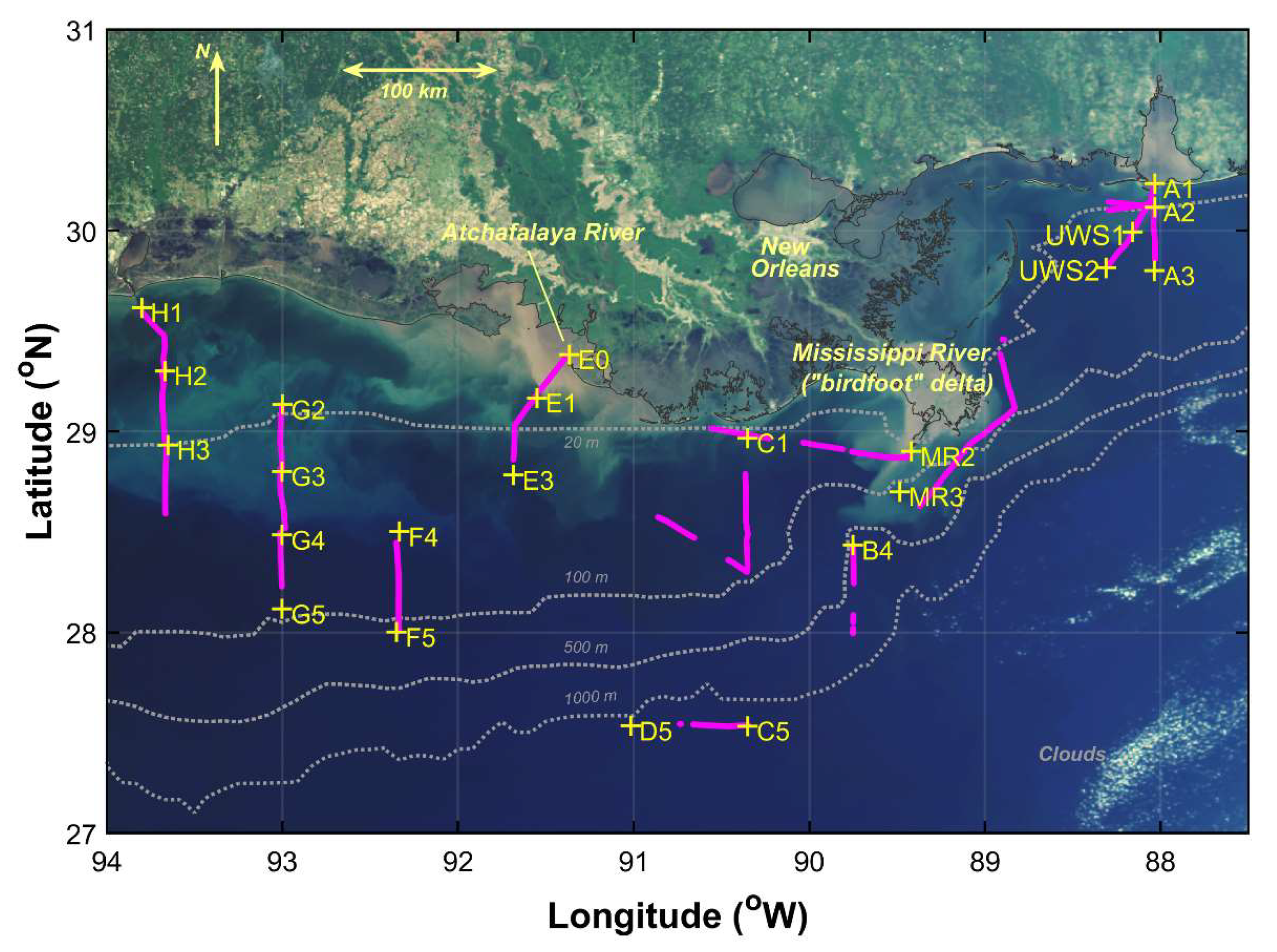
Observations were conducted from 20 April to 1 May 2009 aboard the R/V Cape Hatteras in the northern Gulf of Mexico as part of the GulfCarbon program. Sampling included underway and profiling radiometry as well as vertical profiles of conductivity, temperature, and depth (SBE 49 CTD, Seabird, Inc., Bellevue, WA, USA). Water samples were collected at selected stations (Figure 1) using 10 L Niskin bottles and subsequently filtered for particulate absorption, phytoplankton pigments, and nutrient analyses. Where conditions were suitable, underway above-water hyperspectral reflectance measurements were conducted as a sampling station was being approached or upon departure to allow comparison to instrument vertical profiling and water sample measurements at the station location. Additional above-water reflectance measurements include those coinciding with underway water sample collections (labeled as “UWS#”) or other underway surveys (referred to as runs) varying in duration (Figure 2). The sampling stations were grouped into four water types—estuarine, inner shelf, mid shelf, open ocean—based on a cluster analysis of temperature, salinity, chlorophyll-a (Chl-a) concentrations, suspended particulate matter, and bathymetry [12]. We identified the river plume–ocean mixing zone based on strong horizontal gradients in surface salinity as well as transitions in optical properties of the water.

Figure 1.
Sampling stations (yellow “+”) and tracks for underway hyperspectral radiometry observation runs (magenta) overlaid on a mapped “true color” image acquired with MODIS Aqua on 14 April 2009.

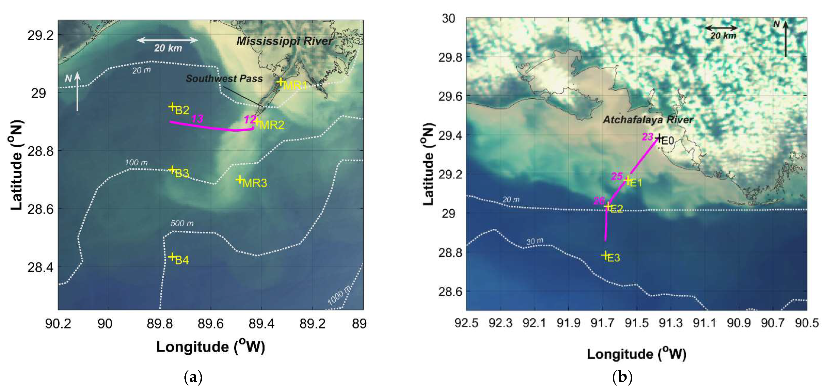
Figure 2.
Sampling stations (yellow “+”) and tracks (magenta lines with run numbers) for underway hyperspectral radiometry observations (magenta) overlaid on mapped “true color” images acquired on the same day of sampling: (a) Mississippi River (22 April 2009); (b) Atchafalaya River (24 April 2009).
2.2. Water Sample Analysis
Nutrient analyses and spectral absorption coefficients of particulate matter were determined as described in [19], with the exception that the method of Stramski et al. (2015) was used for pathlength amplification correction of particulate absorption [20]. Sea surface temperature and salinity measurements were obtained from the shipboard flow-through system using a SeaBird SBE 21 SeaCAT thermosalinograph.
2.3. Tidal and Water Level Data
Tidal and water level data for the Mississippi River plume, obtained from the NOAA Tides & Currents station 8760922—Pilots Station East, S.W. Pass, LA, USA [21], were used to determine tidal conditions during underway sampling runs at the Mississippi (Runs 12 and 13, 22 April 2009, 1600–1800 UTC) and Atchafalaya (Runs 23–26, 24 April 2009, 1730–2100 UTC) river plumes. In both cases, sampling occurred during ebb tide conditions.
2.4. Satellite Imager
Moderate Resolution Imaging Spectroradiometer (MODIS) Aqua ocean color satellite imagery was acquired from the NASA Ocean Biology Distributed Active Archive Center (NASA). Level 0 files were processed to quasi-250 m resolution Level 2 remote sensing reflectance products using the SeaDAS data analysis system version 8.0. To ensure a high degree of quality, pixels were excluded if they were associated with the following quality control flags as per Lohrenz et al. (2018) [22]: atmospheric correction failure, land, sun glint, high radiance, large sensor viewing angle (>60°), stray light, cloud/ice, high solar zenith angle, low water-leaving radiance (low nLw_555), questionable navigation, Chl-a >64 or <0.01 mg m−3, suspicious atmospheric correction, dark pixel (scan line error), and navigation failure. Matchups between satellite observations and ship-based underway measurements were retrieved for 3 × 3-pixel windows co-located with observations made within ±6 h of image acquisition.
2.5. Above-Water Reflectance
Above-water, underway, hyperspectral radiometry measurements were made using a Satlantic, Inc. (now available through Seabird Inc., Bellevue, WA, USA) HyperSAS hyperspectral optical remote sensing system in combination with additional discrete radiometers extending into the UV. The HyperSAS suite included two HyperOCR-R radiance sensors for measurement of total above-water (Lt) and sky radiance (Lsky), both in units of μW cm−2 nm−1 sr−1, and two HyperOCR irradiance sensors for measurement of downwelling surface spectral irradiance (Es, μW cm−2 nm−1) in both UV (350–400 nm) and visible (400–800 nm) wavelengths over 166 channels. The field of view for the radiance sensors was 10° in air. The irradiance sensors exhibited a cosine response within 3% for 0–60° and within 10% for 60–85° incident angles. Additionally, integrated into the optical system were discrete sensors (Satlantic OCR) with bands at selected UV wavelengths (305, 325, 340, 380 nm for Lt, Lsky, and Es) and one red wavelength (670 nm for Lt and Lsky only). The radiometers were mounted on the O2 deck at a 90° angle relative to the ship’s heading along the side railing at an above-water height of approximately 8 m (Figure S1). The Lt sensor viewing angle was 35° from nadir and the Lsky sensor was oriented 125° from nadir. A Satlantic Tilt/Heading Sensor was mounted together with the radiance sensors. The two HyperOCR downwelling irradiance (Es) sensors were mounted on a frame at the level of the O2 deck. A GPS provided ship’s heading and speed.
Data during cruise sampling were acquired using Satlantic SatView 2.8.2 software and saved as Level 1 raw files. Sampling was limited generally to between 10 a.m. and 4 p.m. local time. Sampling frequencies varied adaptively; integration times ranged from ~0.1 to 0.5 s. The data consist of measurements that were conducted as a sampling station was being approached or upon departure to allow comparison to instrument vertical profiling and water sample measurements at the station location. Additional Rrs measurements include underway surveys that varied in length and duration, hereafter referred to as “runs”. Sampling data files were saved regularly while underway, and whenever sampling was interrupted for water sampling and vertical profiling on station. The raw files were subsequently processed to Level 2 using Satlantic SatCon-1.5.5 processing software in conjunction with instrument calibration files. The Level 2 data files were compiled and subsequently processed further using Matlab® (see data availability section).
HyperOCR radiances and irradiances were dark-corrected using linearly interpolated dark observations. For computations of reflectance, downwelling surface irradiance (Es) and sky radiance (Lsky) were interpolated to coincide with total water radiance (Lt) times and wavelengths. Data were filtered to remove effects of episodic sun glint as well as more periodic variations associated with sky glint and sea foam from the ship’s wake [23,24,25]. Filtering of the HyperOCR Lt observations was initially accomplished by determining the slope of Lt(λ) normalized to Lt(770) over the range of 770–800 nm (where λ corresponds to wavelength) and omitting Lt spectra for which the slope was less than −0.007 λ−1 or greater than 0.01 λ−1. Additionally, data were further filtered by omitting all but the lowest 10% out of every 60 spectra based on the median values within the wavelength range 775–785 nm. For the discrete OCR Lt UV data, filtering was accomplished by omitting out of every 60 observations all but the lowest 5% of spectra at 670 nm.
Remote sensing reflectance (Rrs, sr−1) was estimated using an approach modified from [26]. Specifically, Lt values were adjusted for Lsky reflectance as follows to determine water leaving radiance (Lw):
where the value of ρ was determined using the approach of Ruddick et al. (2006) [27]. This estimation of ρ adopts a constant value of 0.0256 for cloudy sky conditions and adjusts for wind speed in clear sky conditions. A ratio of Lsky(750)/Es(750) was used to distinguish clear versus cloudy sky conditions. Values greater than or equal to 0.05 corresponded to cloudy conditions, and a constant value of ρ = 0.0256 was used. Otherwise, ρ was determined as follows:
where W corresponds to wind speeds in m s−1. Wind speeds were obtained from the NOAA National Data Buoy Center meteorological buoy 42040, located 63 nautical miles South of Dauphin Island, AL (https://www.ndbc.noaa.gov/station_page.php?station=42040, accessed on 20 August 2021). The buoy wind speeds were linearly interpolated to match the sampling intervals of Lt and the interpolated Lsky data prior to estimation of . Remote sensing reflectance was subsequently calculated as:
The calculated Rrs data required further filtering to account for ship movement and changing orientation relative to the sun’s plane [25]. The pitch and roll sensor data were linearly interpolated to match the sampling intervals of Lt data, and data were excluded for pitch or roll angles greater than 5°. Data collected for solar zenith angles greater than 80° or less than 10° were also excluded. The sensor azimuth angle relative to the solar plane (RelAz) was estimated by initially calculating the solar azimuth angle for the given date, time, and location and using the ship’s heading plus the appropriate 90° offset of the sensors to determine RelAz. Nominally, RelAz values of 90–135° are preferred as a means of minimizing the effects of sun glint and contamination effects by ship superstructure [25,26].
The Rrs data were further filtered to remove outliers by eliminating spectra with Rrs values less than −0.1 or greater than 0.08 and subsequently applying a median filter to Rrs(555) (or Rrs(380) in the case of the discrete OCR Rrs observations) and excluding spectra differing by more than one scaled median absolute deviation (MAD). The filter was applied with a sampling window size of 20 min for comparisons of underway measurements to station data and 5 min for runs or the full duration of the run for shorter sampling sessions. These latter data filtering steps generally resulted in an omission of a relatively small percentage (<10%) of the remaining data but did improve overall data quality.
To additionally account for residual glint, we applied a wavelength-independent baseline correction. The method for determining the correction depended on whether the spectral minimum was in the UV or infrared regions, as represented by the Rrs(380)/Rrs(780) ratio. For values of the ratio greater than or equal to one (generally true for shelf and ocean stations), baseline corrections were applied by adjusting Rrs spectra such that the value at Rrs(780) was zero. Since measurements of Rrs(780) were not available for the discrete OCR measurements, the discrete Rrs values were adjusted so that the mean values of discrete Rrs(380) agreed with the mean Rrs(380) determined with the HyperOCR sensors. For locations in turbid coastal waters, non-zero reflectance in the infrared may be encountered (e.g., [27]), and Rrs(380)/Rrs(780) values of less than one are possible. For these cases, an exponential of the form
was fit to the 350–450 nm portion of each spectrum and used to determine an extrapolated value for Rrs(340), which was subsequently subtracted from all discrete Rrs bands as a baseline correction. This approach assumed that for such turbid, coastal conditions, Rrs in the UV approached zero. Finally, an additional filter was applied to omit the baseline-corrected spectra with Rrs values less than −0.01.
2.6. Profiling Radiometry
Vertical profiles of hyperspectral radiometry measurements were acquired at selected stations using a Satlantic, Inc. HyperPro hyperspectral optical remote sensing system. The profiling radiometer instrument included a HyperOCR radiance sensor for measurement of upwelling radiance (Lu) in units of μW cm−2 nm−1 sr−1 and downwelling irradiance (Es, μW cm−2 nm−1) in both UV (350–400 nm) and visible (400–800 nm) wavelengths over 166 channels. The instrument was also equipped with internal tilt and pressure sensors. The field of view of the radiance sensor was 8.5° in water.
Data during cruise sampling were acquired using Satlantic SatView 2.8.2 software and saved as Level 1 raw files. Sampling was limited generally to between 10 a.m. and 4 p.m. local time. Sampling frequencies varied adaptively; integration times ranged from ~0.06 to 2.0 s. Sampling was conducted while the ship was on station. The profiler was deployed off the sun-facing side of the ship and allowed to drift away from the ship to a distance of approximately 25 m. A pressure tare was acquired while the sensor was held near the surface. Repeated profiles were made (variable number depending on depth and station conditions), and sampling data files were saved after each profile. The raw files were subsequently processed to Level 2 using the Seabird Scientific Prosoft 7.7.19 processing software in conjunction with instrument calibration files. The Level 2 data files were compiled and subsequently processed further using Matlab® (see data availability section).
HyperOCR radiances and irradiances were dark-corrected using linearly interpolated dark observations. For computations of reflectance, all radiometric measurements were interpolated to coincide with the downwelling irradiance (Ed, μW cm−2 nm−1) sampling frequency and wavelengths. Both downwelling irradiance (Ed) and upwelling radiance (Lu, μW cm−2 nm−1 sr−1) were adjusted for variations in surface irradiance during the profile by normalizing values to surface downwelling irradiance (Es) at the corresponding sampling times t and multiplying by the initial value of Es at time for the profile [25]. Values of and , where z is depth, were extrapolated to the below the surface to estimate and by applying a least squares fit of the natural log of the radiometric quantities versus depth. This interpolation was done over the upper 5 m for station depths less than 10 m, over the upper 10 m for stations depths between 10 and 40 m, and over the upper 40 m for station depths greater than 40 m.
Values of were converted to above-water surface values, , following Zibordi et al. (2012) [28]:
and remote sensing reflectance (Rrs, sr−1) was estimated as:
where the value of was estimated as the value of at time .
Quality checks of the data were performed following procedures as outlined in Zibordi et al. (2012, 2019) [25,28]. For , quality indices included the value of r2 determined from the regression of log-transformed at depths z and the visual inspection of the Rrs data. If r2 values less than 0.7 were found, then the profile was omitted. Rrs spectra were visually inspected for non-homogeneity, and outlying spectra were omitted. Additional quality filtering included excluding data for pitch or roll angles greater than 5° and profiling velocities less than 0.01 ms−1. The Rrs data were further filtered to remove outliers by applying a median filter to Rrs(555) and excluding spectra differing by more than two scaled median absolute deviations (MAD). The filter was applied only to those stations with 5 or more profiles, and a sampling window size of 5 was used. The omission of data due to filtering varied between stations. For offshore stations, generally fewer spectra were omitted. For some of the coastal stations where conditions were more challenging for profiling, as much as 40–60% of the spectra were omitted. To additionally account for residual glint, we applied a baseline correction by adjusting Rrs spectra such that the mean Rrs value for the wavelength range of 750–780 nm was zero.
2.7. Phytoplankton Absorption ( ) and Particulate Backscattering ( ) Retrieval
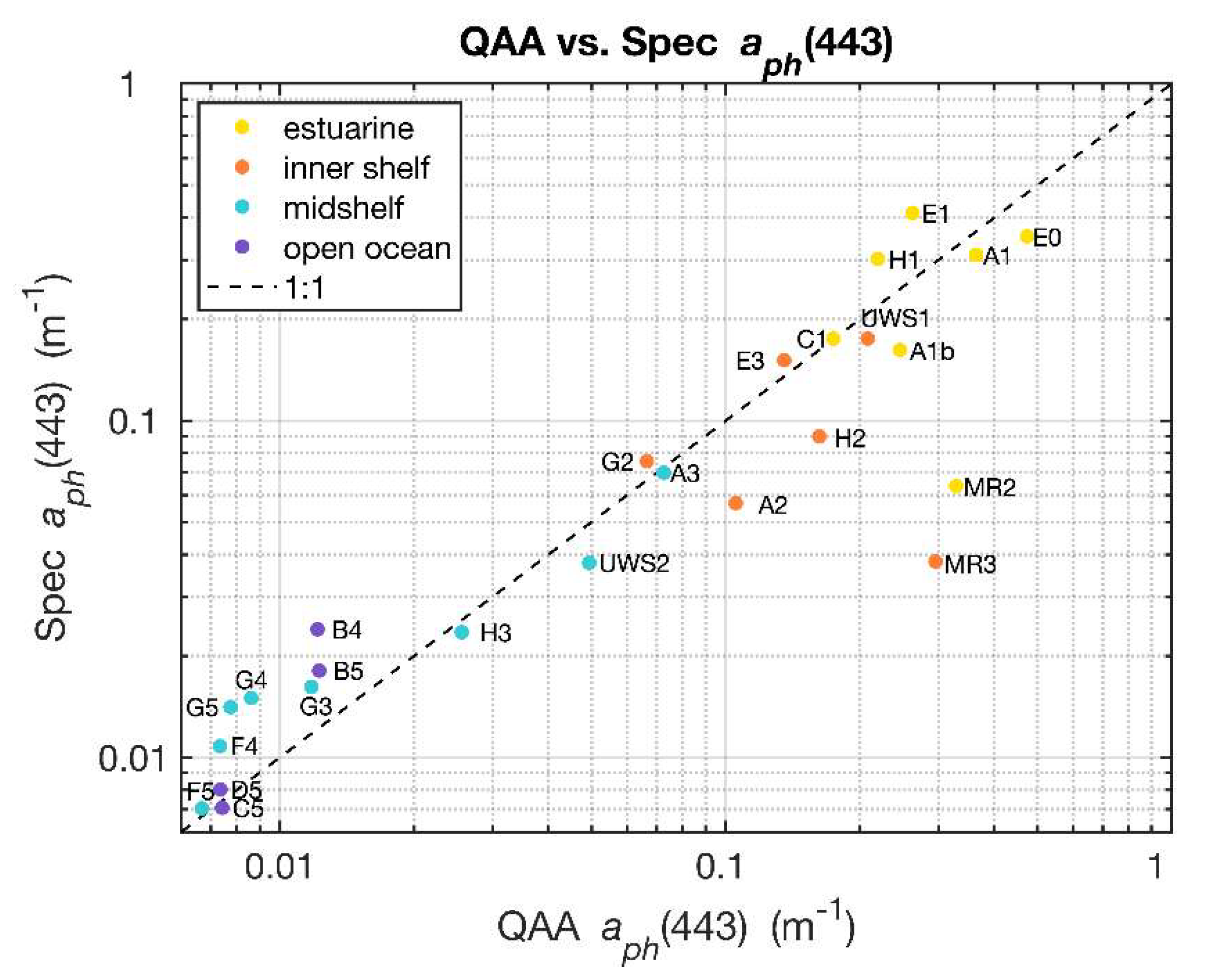
The Quasi-Analytical Algorithm (QAA_v6) [29] was applied to the remote sensing reflectance measurements obtained from HyperSAS to retrieve absorption coefficients of phytoplankton pigments () and particulate backscattering () from remote sensing reflectance spectra. Because of its applicability to both case 1 (open ocean) and case 2 (coastal/estuarine) waters as verified by Zhan et al. (2020) [30], the QAA_v6 was chosen for our study of sub-km scale spatial variabilities across the river plume–ocean mixing zone. The algorithm was applied to individual reflectance spectra acquired in the vicinity of the sampling stations as well as for the underway runs to retrieve and for the wavelength range of 350–750 nm. A comparison of (443) from filter pad measurements determined from near surface samples using the quantitative filter pad technique (QFT) [12] and that from underway reflectance, retrieved using the QAA_v6, in the same vicinity yielded good agreement (Figure 3). Some outliers with low Spec (443) were evident, such as stations MR2 and MR3, which may be due to the direct influence of the Mississippi River outflow where the thin surface layer may have been disrupted by ship motion and sampling activities.

Figure 3.
Values of QAA_v6 derived from HyperSAS Rrs were generally comparable to determined from spectrophotometer estimates of filter pad absorption. Data labels indicate station names and colors indicate water type of the station as shown in the legend.
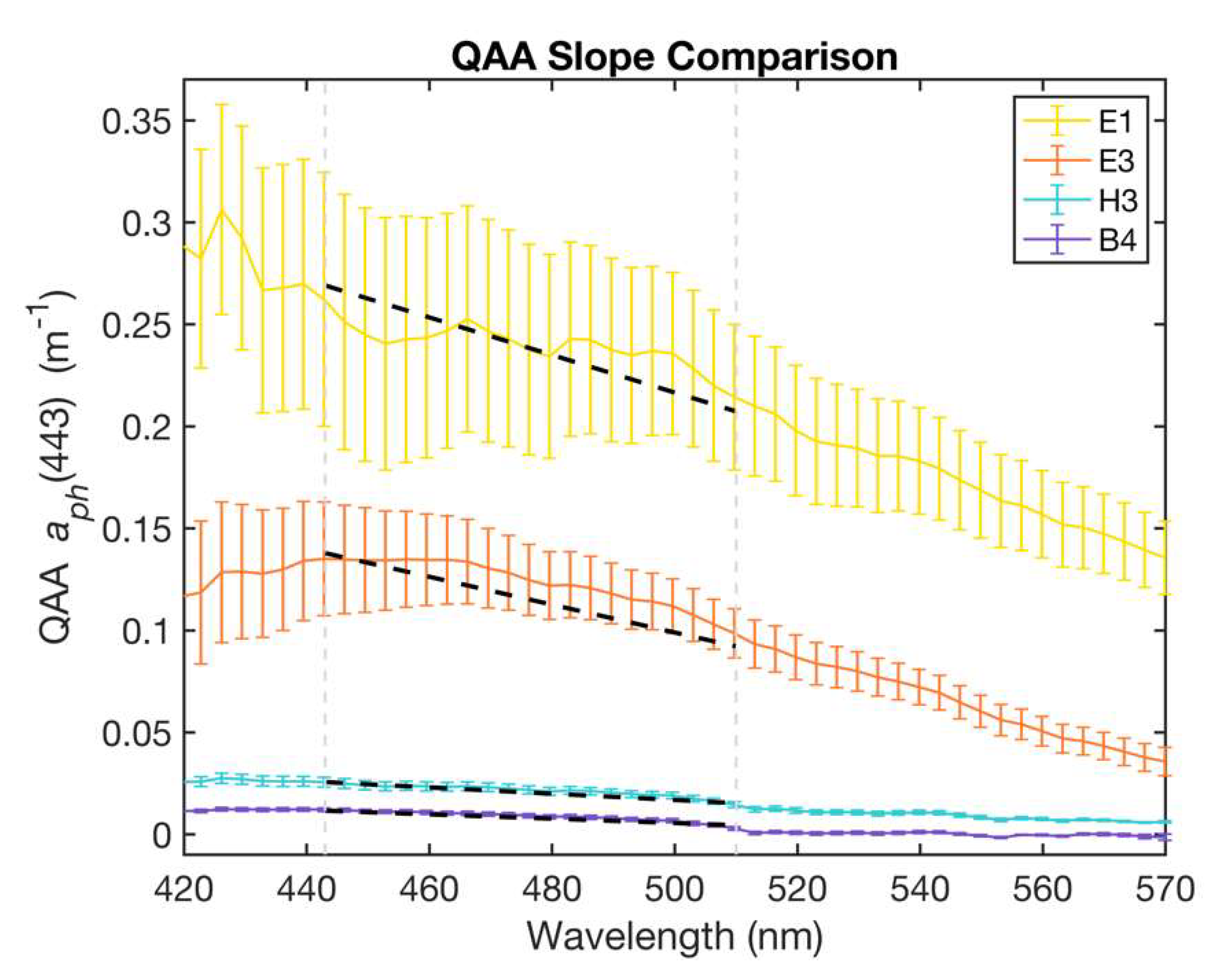
The spectral shape and absolute magnitude of the phytoplankton absorption spectra between 400 and 550 nm (blue-green region) is influenced by Chl-a and accessory pigment absorption, which is, in turn, related to differences in phytoplankton taxa and cell size [6,8]. Thus, the spectral slope of phytoplankton absorption in the range of 443–510 nm was used as an index of phytoplankton size (Figure 4), as previously described by Hirata et al. (2008) [6]. They demonstrated relationships between phytoplankton absorption at (443) and the spectral slope (SH):
with higher slope values corresponding to higher values of (443) and Chl-a. Thus, microplankton were found to have the largest (443) and SH values, while picophytoplankton were associated with smaller ranges of (443) and SH.
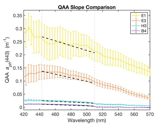
Figure 4.
Absorption spectra for four representative stations, E1 (estuarine), E3 (inner shelf), H3 (mid-shelf), and B4 (open ocean) with linear least squares fit (black dashed lines) depicting the spectral slope for each station between 443 and 510 nm (delineated by grey dashed lines). Steeper slope values were associated with microphytoplankton-dominated communities in contrast to the flatter slopes indicative of picophytoplankton-dominated waters. Error bars represent one standard deviation above or below the mean.
For some sampling stations, particularly those in very turbid conditions, the peak in QAA_v6-derived phytoplankton absorption, , was found to be shifted to wavelengths longer than 443 nm. We attributed this to the large contribution to total absorption by non-pigmented particles and colored dissolved organic matter to the total optical signal, making the retrieval of phytoplankton absorption sensitive to relatively small uncertainties in non-pigment absorption. Consequently, we computed the spectral slope (here designated as S) by applying a linear least squares fit to the vs. relationship only for the portion of the spectrum between the maximum spectral value of and 510 nm. This approach had the advantage over Equation (7) of utilizing the full spectral information for the slope wavelength range rather than just the endpoints. Slope values were subsequently expressed as the natural logarithm of the absolute value of S () to improve linearity.
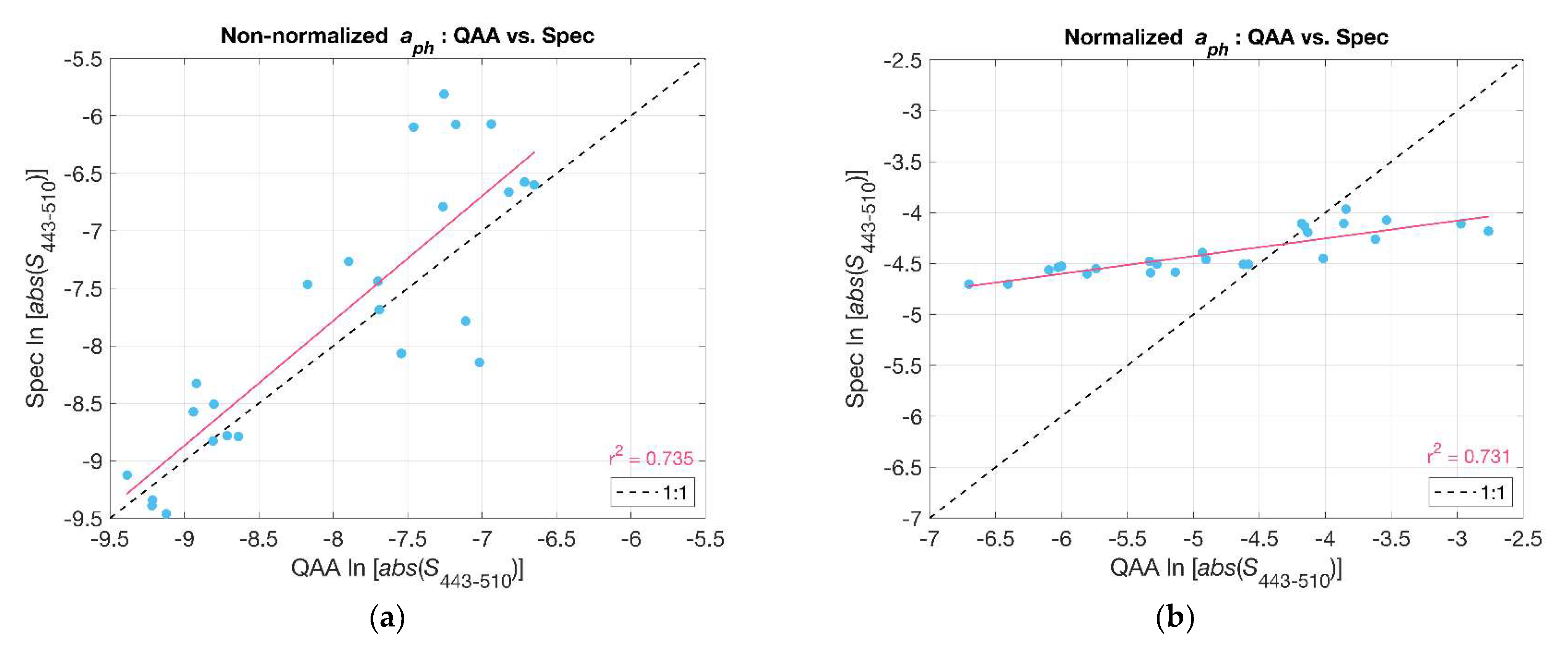
In contrast to Hirata et al. (2008) [6], Ciotti et al. (2002) [8] computed the spectral slope for values that were normalized to the mean of for the given wavelength range. Normalizing the absorption spectra reduces the dependence of the slope on the magnitude of Chl-a such that differences in slope are primarily due to spectral shape as opposed to both shape and magnitude in the case of the non-normalized spectra [6]. We compared the values of S (i.e., ) for both normalized and non-normalized phytoplankton absorption spectra acquired from filter pad measurements and as derived from Rrs using the QAA_v6 (Figure 5). In both cases, there were significant relationships (r2~0.73). However, the normalized slopes retrieved from reflectance using the QAA_v6 varied over a wider range and deviated from a one-to-one relationship with the spectrophotometric measurements. We contend that this was due to a slight negative bias in QAA_v6 at low values and a slight positive bias at high values (cf. Figure 3). Our modified Hirata et al. (2008) [6] approach appeared to be less sensitive to these biases, and we therefore chose to use that approach as described above for subsequent analyses.
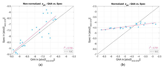
Figure 5.
Slope indices () were compared: QAA_v6-derived versus spectrophotometer-derived non-normalized (a) and normalized (b). The red lines represent the linear least squares fit to the data. The black dashed line is the one-to-one relationship.
2.8. Phytoplankton Pigment Analysis
Methods for sampling and high-performance liquid chromatography (HPLC) analyses of phytoplankton pigments were previously described by Chakraborty and Lohrenz (2015) [12]. The Chl-a normalized concentrations of the major diagnostic pigments were grouped according to the four water regimes (estuarine, inner shelf, mid shelf, open ocean) and were compared to the distribution of size fractions for the respective regimes.
The diagnostic pigment analysis (DPA) method of Uitz et al. (2006) [7] was applied to near surface pigment concentrations of total chlorophyll and seven accessory pigments for each sampling station. The DPA categorizes phytoplankton based on pigment weighting into three size classes—microphytoplankton, nanophytoplankton, and picophytoplankton. For the purposes of our comparison of PSCs as derived from remote sensing reflectance measurements to those from the DPA, we categorized phytoplankton communities to be either microphytoplankton-dominated (micro) or picophytoplankton-dominated (pico). Here, we used the term “picophytoplankton-dominated” to refer to the combined nanophytoplankton and picophytoplankton fractions as categorized by the DPA.
3. Results
3.1. Intercomparison of Remote Sensing Reflectance Measurements
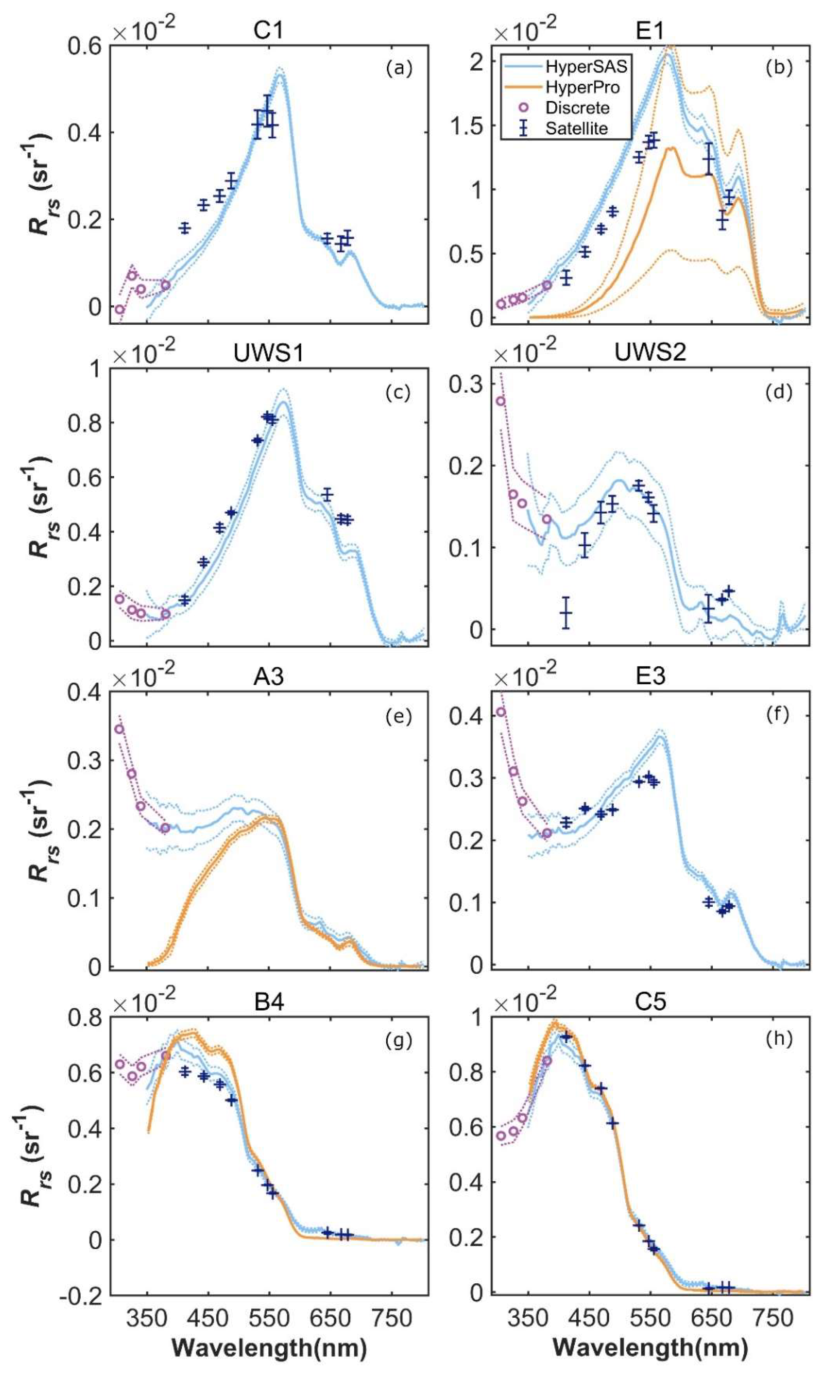
An intercomparison of remote sensing reflectance (Rrs) determined using the shipboard sensors (HyperSAS and HyperPro) and MODIS Aqua-derived Rrs was possible at selected stations and revealed reasonable agreement, with some differences particularly for some mid- and inner shelf stations (Figure 6 and Figure S2). HyperSAS and satellite Rrs measurements agreed reasonably well at estuarine stations C1 and E1 and inner shelf station USW1 (Figure 6a–c). HyperPro Rrs at station E1 was lower and more variable than the HyperSAS and satellite Rrs estimates. This could be due to the extremely high turbidity conditions at E1, which was located in the Atchafalaya plume and characterized by a thin, low salinity surface layer and very high reflectance. Such conditions are difficult to sample with in-water radiometry due to the strong, near-surface vertical gradients. At mid-shelf stations UWS2 and A3 (Figure 6d,e), HyperSAS Rrs at wavelengths below 500 nm tended to be higher than that observed for MODIS Aqua (UWS2) or HyperPro (A3) Rrs estimates. Additionally, discrete wavelength measurements in the UV portion of the spectrum for mid-shelf stations UWS2 and A3 and inner shelf station E3 (Figure 6d–f, respectively) exhibited increasing values with decreasing wavelength. For open ocean stations B4 and C5 (Figure 6g,h), there was generally good agreement among all methods and across all wavelengths.

Figure 6.
Comparison of HyperSAS, HyperPro, and MODIS Aqua Rrs at selected stations, including estuarine stations C1 (a) and E1 (b), inner shelf stations UWS1 (c) and E3 (f), mid-shelf stations UWS2 (d) and A3 (e), and open ocean stations B4 (g) and C5 (h).
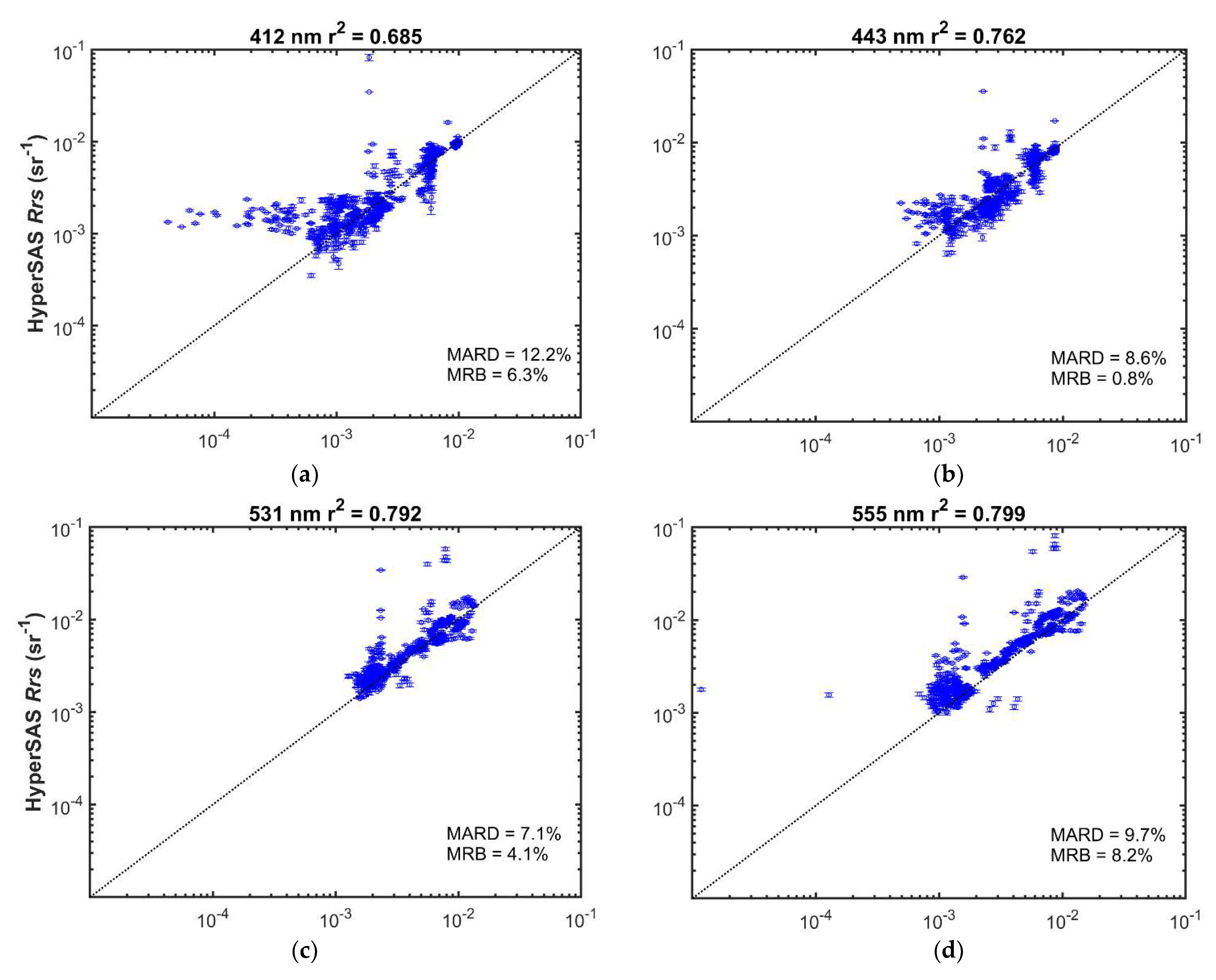
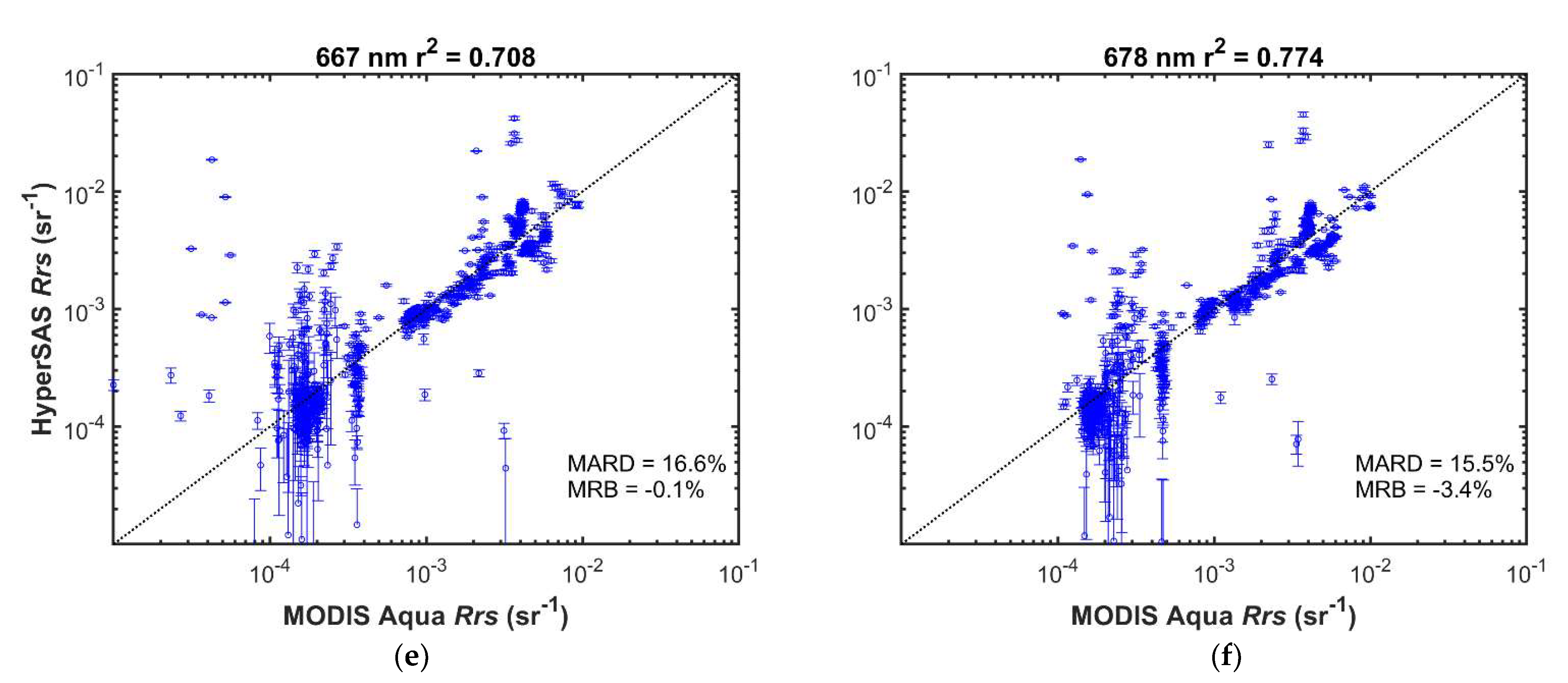
MODIS and HyperSAS Rrs measurements were generally well correlated (r2 = 0.68 or greater; Figure 7 and Figure S3). Mean absolute relative differences ranged from 7 to 17%. Mean relative biases were less than 10% and were positive for wavelengths 645 nm and below, but slightly negative for longer wavelengths. Biases were likely a consequence of higher variability in the HyperSAS measurements as well as potentially larger uncertainties in satellite-derived Rrs at shorter wavelengths [31,32]. A positive bias in HyperSAS Rrs at low values for 412 nm was evident (Figure 7a) and could be due to surface glint effects or reflected light off ship superstructure. Poor agreement at low reflectance seen for 412 nm (Figure 7a), 667 nm (Figure 7e), 678 nm (Figure 7f), and 645 nm (Figure S3d) may also be attributed to low signal-to-noise at the low reflectance values.
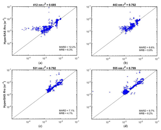
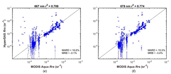
Figure 7.
Comparison of HyperSAS and MODIS Aqua Rrs at selected wavelengths: (a) 412 nm; (b) 443 nm; (c) 531 nm; (d) 555 nm; (e) 667 nm; (f) 678 nm. Error bars represent + one standard deviation of the intrapixel variability in HyperSAS Rrs. The dotted diagonal line is the 1:1 relationship. MARD = mean absolute relative deviation; MRB = mean relative bias.
Possible sources of differences when comparing the two Rrs measurements could also be a consequence of differences in time of satellite overpass and time at which HyperSAS measurements were taken. Intrapixel variability, as indicated by the standard deviation in HyperSAS Rrs measurements (Figure 7), was generally small (mean values less than 0.0002 sr−1). Higher relative intrapixel variability was evident for the longer wavelengths at low values.
3.2. Pigment and PSC Distribution
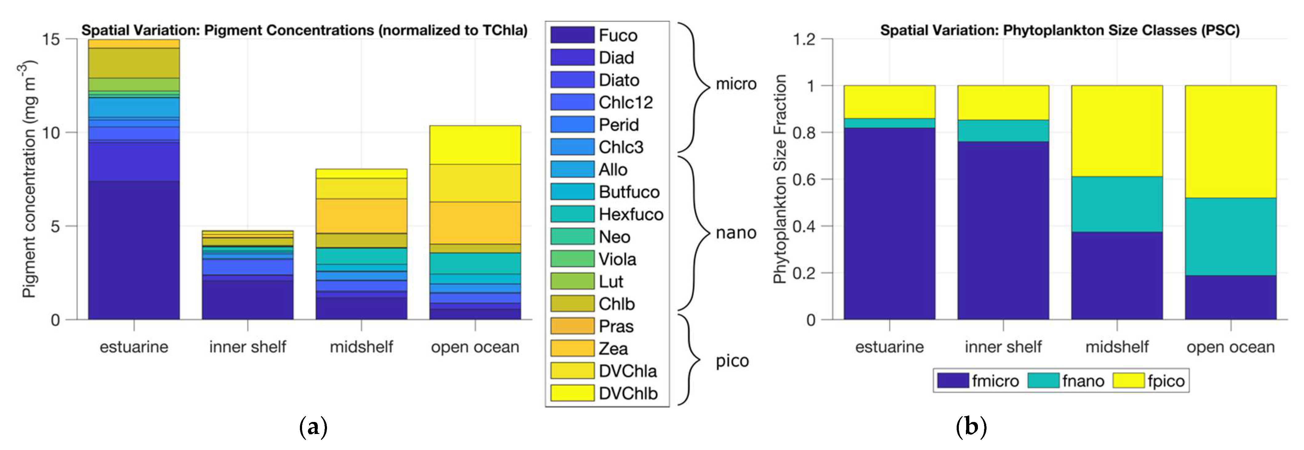
Using pigment data from HPLC analysis of water samples, a trend of increasing picophytoplankton-associated pigments was seen from estuarine to open ocean waters (Figure 8). The transition also indicated a decrease in microphytoplankton-associated pigments. The phytoplankton size fractions obtained from the DPA exhibited a similar trend with increasing picophytoplankton and nanophytoplankton fractions and decreasing microphytoplankton fractions from estuarine to open ocean waters (Table S1).
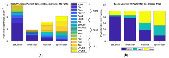
Figure 8.
(a) Concentration of 17 diagnostic pigments as measured at stations of four different water types—estuarine, inner shelf, mid-shelf, and open ocean. (b) PSC distribution across the four water types derived using the DPA [7].
3.3. Comparisons of Optical and Pigment-Based PSC
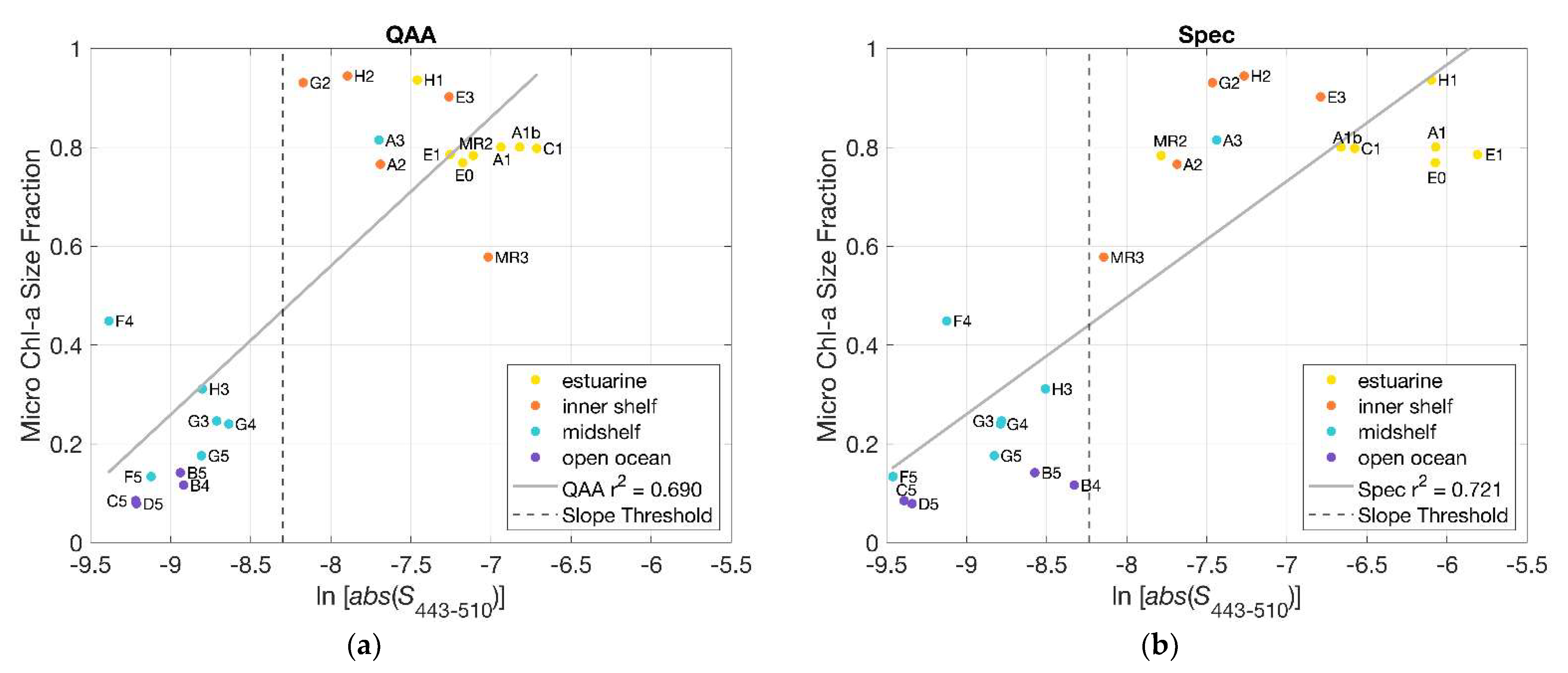
To verify the use of hyperspectral slope retrieval as a determinant of spatial distribution of phytoplankton size classes (PSCs), we compared the fraction of microphytoplankton present at each station to the slope indices (for the non-normalized derived from applying the QAA_v6 to the HyperSAS Rrs (Figure 9a). It was seen that slope indices more negative than the threshold value of −8.3 were associated with stations with a relatively low microphytoplankton size fraction (<50%). Alternatively, slope indices that were less negative than the threshold value were characterized by high microphytoplankton size fractions (>50%). A comparison of the relationship for slopes derived for from filter pad (Spec) measurements (using the QFT, Section 2.7) yielded similar findings (Figure 9b and Figure S4), with comparable values of the coefficient of determination, r2. Mean-normalized slope indices for both filter pad and QAA_v6-derived also exhibited significant relationships to microphytoplankton size fractions, although with slightly lower r2 values for the QAA_v6-derived slope indices (Figure S5). Similar trends were seen in comparisons of nanophytoplankton, picophytoplankton, and picophytoplankton + nanophytoplankton size fractions to slope indices for both QAA_v6- and spectrophotometer-derived (Figures S6–S8).

Figure 9.
(a) Slope indices (), calculated for non-normalized retrieved from HyperSAS Rrs with the QAA_v6 (blue), were plotted in relationship to the microphytoplankton size fraction (determined using pigment concentrations, [6]) for all stations; (b) as in (a) but for slope indices ( ) derived from spectrophotometer measurements of .
This comparison revealed a clear distinction between estuarine + inner shelf stations and mid-shelf + open ocean stations. Estuarine + inner shelf stations were dominated by microphytoplankton, whereas mid-shelf + open ocean stations (apart from station A3) were dominated by picophytoplankton. This result provided a basis for the use of slope indices retrieved from QAA_v6-derived from hyperspectral Rrs as a proxy for the determination of dominant PSCs. There was some scatter in the relationship between phytoplankton size fractions and slope indices (, particularly for the estuarine and inner shelf stations (upper right corner of Figure 9a), and this may at least partially be attributable to higher uncertainties in the QAA_v6 retrievals in turbid coastal waters.
To evaluate the performance of the approach for hyperspectral versus multispectral data, slope indices (), calculated for non-normalized retrieved using the QAA_v6 from the full spectral HyperSAS Rrs (blue) versus that only for the MODIS Aqua wavelengths, were examined in relationship to the microphytoplankton size fraction for all stations (Figure S9). While both relationships were significant, the relationship for the hyperspectral observations had a higher r2 than that for the multispectral (0.69 vs. 0.55).
3.4. Comparison of Mississippi and Atchafalaya Plume Features
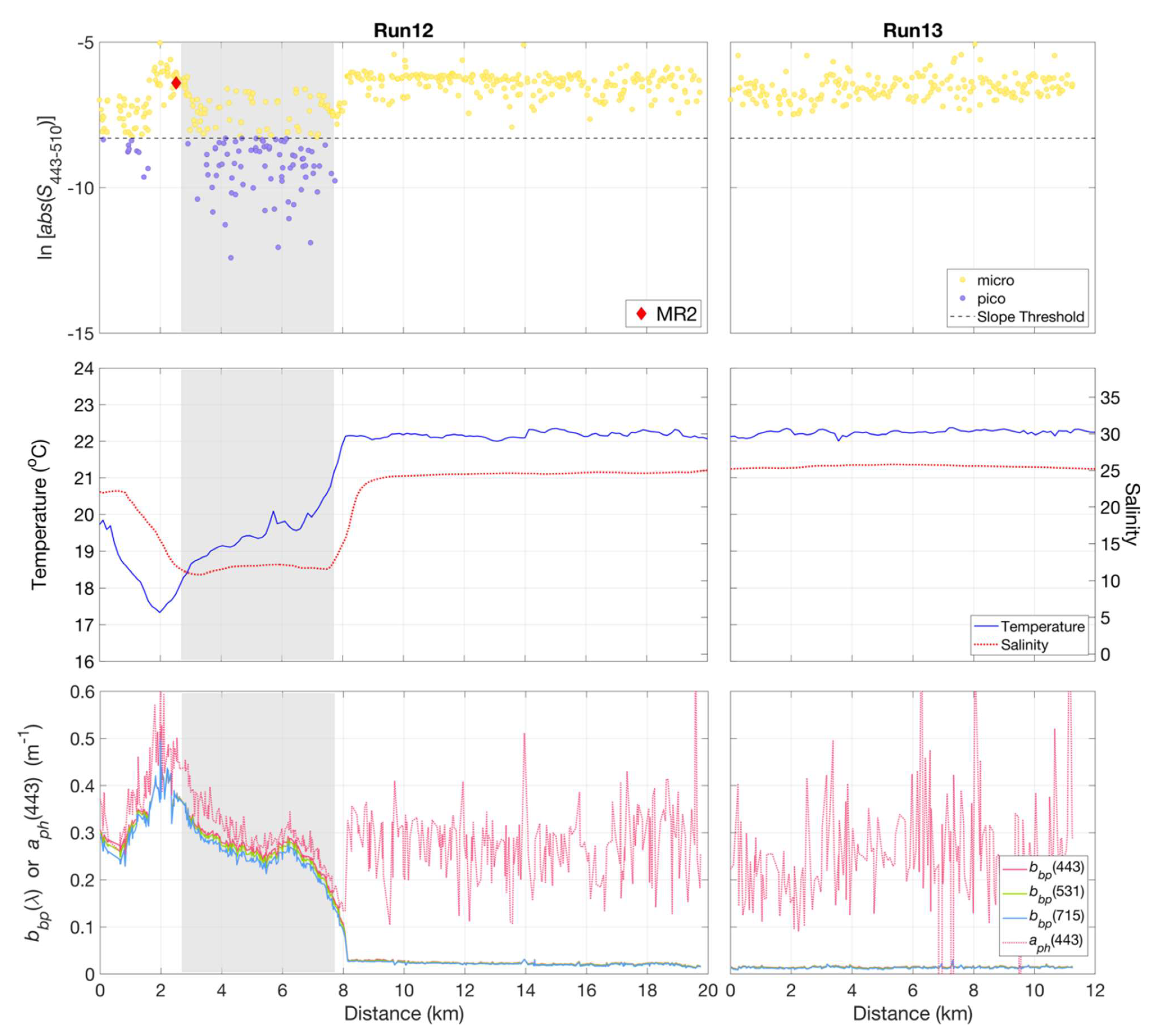
Sub-km scale variations in phytoplankton community composition were observed using underway hyperspectral Rrs measurements in a cross-plume transect near the mouth of the Mississippi River at Southwest Pass (Figure 10). A transition was observed in phytoplankton community composition from a mixed micro- and picophytoplankton population within the Mississippi river plume to one primarily dominated by microphytoplankton beyond the river plume–ocean mixing front (Figure 10, Run 12). Data from inner shelf waters beyond the front were dominated by microphytoplankton (Run 13). The cross-plume variations in the phytoplankton community were clearly related to the strong gradients in temperature and salinity across the plume boundary—and likely influenced by convergence, entrainment, and mixing of fresh and saline water masses.
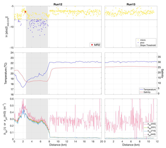
Figure 10.
Variations were observed in slope indices () (top panel), calculated for non-normalized retrieved from HyperSAS Rrs with the QAA_v6, for Runs 12 and 13 across the Mississippi River plume. The plume region was evident in differences in temperature and salinity (middle panel), as well as in particulate backscattering, , and QAA_v6-derived phytoplankton absorption, (lower panel). The shaded grey area indicated the approximate range of the plume core based on its relatively low salinity as compared to surrounding waters. Micro = microphytoplankton-dominated community, pico = picophytoplankton-dominated community.
Particulate backscattering measurements, , as estimated from the QAA_v6, can be considered to be representative of turbidity and particle abundance, while would be representative of variations in phytoplankton pigment biomass. High and variable values of both and were associated with turbid waters within the river plume core. The transect across the plume core was characterized by high values of the index at the plume edge, indicative of a microphytoplankton-dominated community, followed a region of lower values indicating a mixed population of both micro- and picophytoplankton in the low salinity core of the plume. An abrupt decrease in delineated the outer edge of the plume front and a shift from plume to coastal waters, which was also evident in the sharp increase in salinity and temperature. In contrast, values were variable and similar in magnitude to values in the plume. The coastal waters adjacent to the plume were dominated by microphytoplankton.
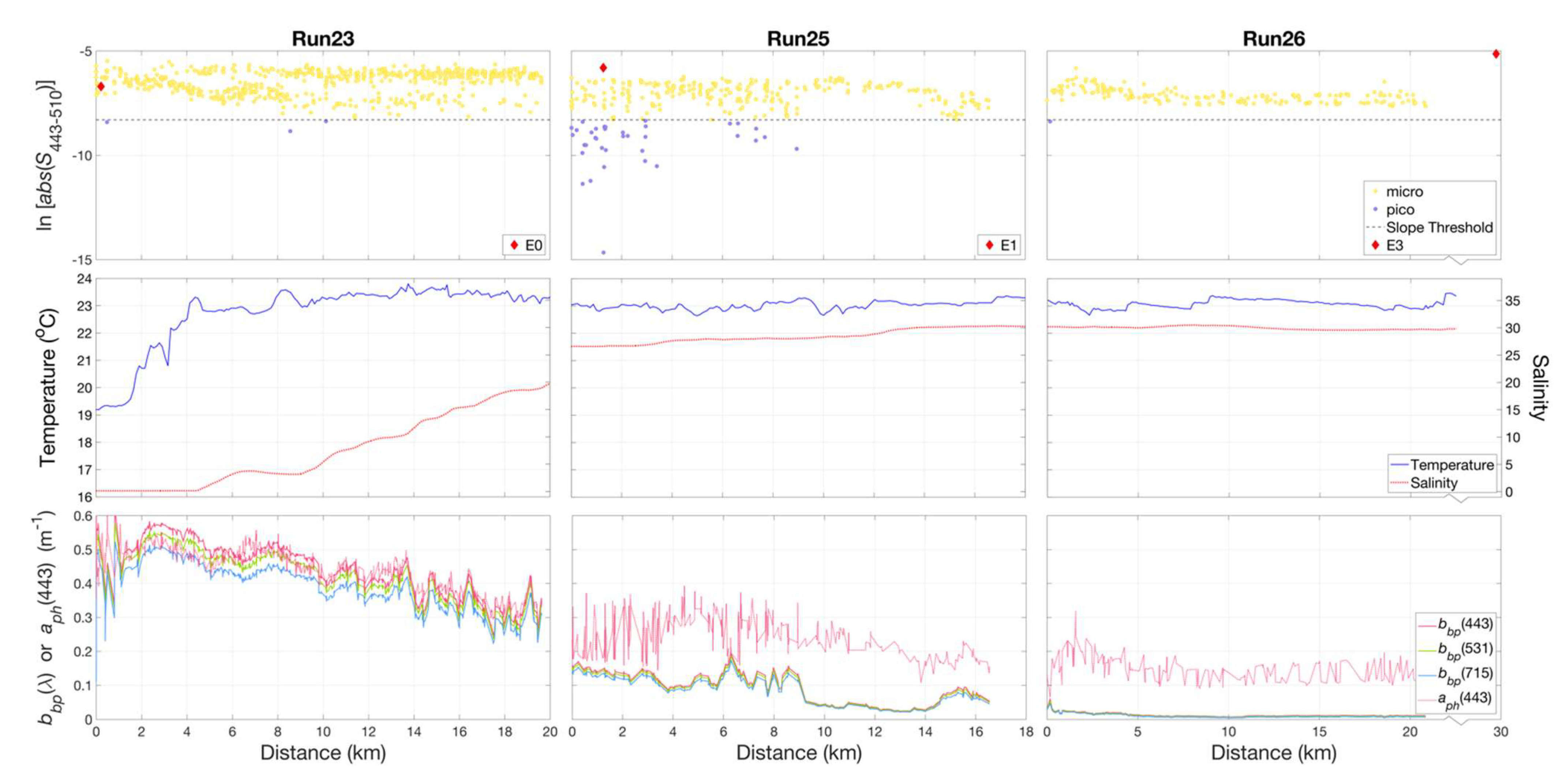
The transect extending offshore along the Atchafalaya River plume (Figure 11) was characterized by increases in salinity and temperature (Run 23) along the river plume–ocean mixing zone. Slope indices were indicative of a microphytoplankton-dominated community throughout the zone. During Run 25, decreasing and variable values of and , accompanied by a slight increase in salinity, were associated with localized patches in which slope indices indicated the presence of both micro- and picophytoplankton-dominated communities. This was seen in two locations during the run, one at 0–3 km and a second from 6 to 9 km, separated by a microphytoplankton-dominated region from 4 to 6 km. These observations coincided with the outer edges of the visible signature of the river plume ocean waters, as evident in Figure 2b. Beyond the mixing zone, we observed a microphytoplankton-dominated community in shelf waters (Run 26).
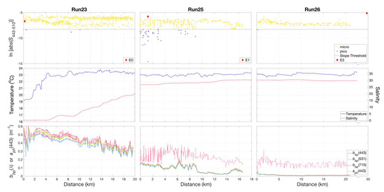
Figure 11.
Variations in slope indices () (top panel), calculated for non-normalized retrieved from HyperSAS Rrs with the QAA_v6, for Runs 23, 25, and 26 along the Atchafalaya River plume. Temperature and salinity (middle panel) exhibited an increase, while particulate backscattering, and phytoplankton absorption, (lower panel) decreased in magnitude with increasing distance along the plume. micro = microphytoplankton-dominated community, pico = picophytoplankton-dominated community.
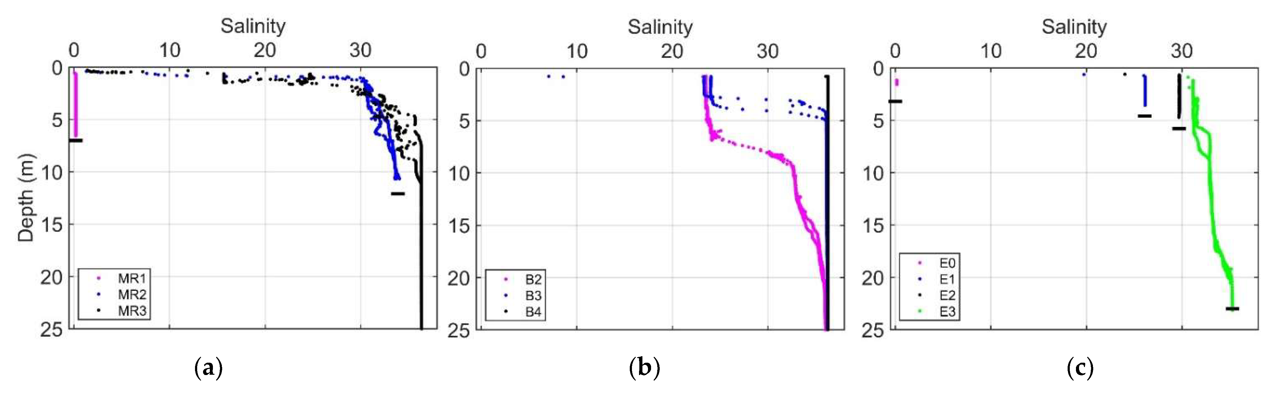
Vertical salinity profiles at stations MR2 and MR3 in the Mississippi River plume region revealed thin surface layers (~1 m) of low-salinity water with a sharp increase in salinity with depth (Figure 12). River stations MR1 (Mississippi) and E0 (Atchafalaya) exhibited uniformly low salinity. Inner shelf stations along the B transect outside the direct influence of the river plume were observed to have intermediate surface salinities around 23 with surface layers ranging about 3–7 m in depth.
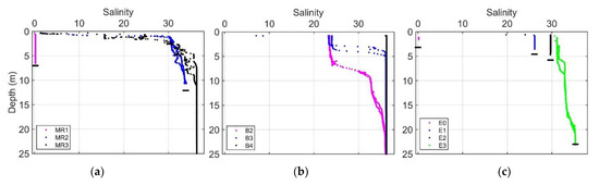
Figure 12.
Vertical salinity profiles within (a) and outside (b) the Mississippi River plume and along the Atchafalaya River plume (c). Horizontal black bars indicate approximate location of the bottom surface. Bottom depths were taken from the ship’s echo sounder (Furuno). In some cases, profiles exceeded the depth reported by the echo sounder, in which case the maximum depth of the profile was used.
4. Discussion
It is well-known that phytoplankton community composition varies from coastal waters, typically dominated by larger phytoplankton, to oceanic waters, which is generally dominated by smaller phytoplankton cells [12,18]. Our work used high spatial resolution hyperspectral reflectance measurements to shed new light on sub-km scale variability in phytoplankton communities associated with dynamic and spatially heterogeneous environmental processes in river-influenced waters.
4.1. Utility of Hyperspectral Underway Reflectance
Our findings have demonstrated the utility of hyperspectral remote sensing to elucidate phytoplankton patterns at high spatial resolution. The environmental conditions in river plumes and interactions with the open ocean are highly dynamic, requiring higher resolution sampling techniques to assess small-scale patterns of variability in phytoplankton communities [33,34]. Although conventional in-situ methods provide key end points of the mixing processes, underway hyperspectral measurements confer the advantage of detecting variations in phytoplankton communities as they occur over strong and temporally variable environmental gradients.
Phytoplankton account for much of the optical variability in visible wavelengths in open ocean waters, and spatial scales of variability are sufficiently large [35], such that multispectral ocean color sensors are able to provide useful information about phytoplankton community composition in such environments. Coastal waters have the added complexity of higher and more variable quantities of dissolved and non-pigmented particulate matter [36]. Thus, the interpretation of multispectral ocean color in coastal environments can be more challenging than in open ocean environments [37]. Our assessment, showing better performance of our modified Hirata et al. approach for hyperspectral versus multispectral data (Figure S9), provided evidence for the benefit of higher spectral resolution for this application. Retrieval of hyperspectral measurements allow for greater precision in the application of methods such as the QAA, and thus, we contend that they have the potential to provide improved estimates of phytoplankton community composition, especially in coastal waters
We also applied our approach to multispectral MODIS Aqua Rrs observations for those stations for which suitable matchups with satellite data were available. However, the relationship between the slope indices determined for derived using the QAA_v6 from the MODIS Aqua Rrs and the phytoplankton size fractions was not significant (r2 = 0.037, data not shown). Other factors in addition to spectral resolution may at least partially explain the poor performance for the satellite data. The satellite matchups were limited to a subset of stations sampled, and intrapixel spatial heterogeneity as well as uncertainties in the atmospheric corrections would introduce additional variability.
We found reasonable agreement among underway hyperspectral remote sensing reflectance observations and both in-water and MODIS Aqua Rrs, particularly for offshore stations where conditions were more uniform. Discrepancies were evident in some cases, in mid- and inner shelf conditions for shorter wavelengths. Systematically higher Rrs observations in the blue and UV wavelengths at some mid- and inner shelf stations were evident for the HyperSAS as compared to either the HyperPro or MODIS Aqua. The increase with decreasing wavelength in Rrs in the UV portion of the spectrum, as seen for some mid-shelf stations, was unexpected. The general understanding is that UV reflectance is quite low in coastal waters [38]. To our knowledge, our measurements are some of the few of UV reflectance made in coastal waters [39]. Anomalously high Rrs measurements in the ultraviolet (UV) spectrum could be an artifact of stray light in the case of hyperspectral sensors [40]. However, this should have been less of a factor for the discrete OCR-UV sensors, which also exhibited this increase in UV Rrs with decreasing wavelength for some stations. Alternatively, an imperfect skylight reflection correction may have been a source of anomalously high Rrs, especially in darker waters where even small errors in the correction can lead to large errors in the UV Rrs. Contamination by reflected light off ship structures or possibly associated with foam or wave facets may have also been a factor. While our application of the phytoplankton size class algorithm would be expected to be relatively insensitive to uncertainties in wavelengths at 412 nm or less, accurate estimates of Rrs in this wavelength range could nonetheless be very useful for certain applications such as characterizing properties of organic matter [41] and possibly certain phytoplankton classes [42]. Further investigation of the sources of variability in UV Rrs is warranted.
Despite some uncertainties in the reflectance measurements, our results were successful in demonstrating the utility of hyperspectral remote sensing reflectance for deriving optical indices of phytoplankton size classes (PSCs). Validation of our approach relied on class size information derived from the Uitz et al. DPA method [7]. We recognize that the DPA’s operational categorization is based on empirical relationships and that pigment composition can vary across and within species. However, the method has been widely used and does generally reflect variations in community composition [43]. A comparative evaluation of the method presented in Devred et al. (2011) was also performed on our data set (data not shown); however, we opted to use the Uitz et al. (2006) method as it performed better for the spectrophotometric data in our region and was consistent with the analysis of Chakraborty and Lohrenz (2015) [7,12,44]. The pigment data set used here has previously been analyzed using CHEMTAX and has been compared to microscopic analyses [12], providing an independent confirmation that the pigment algorithm was representative of actual taxonomic variability in this region. Future development of remote sensing instruments and algorithms as well as their validation using a combination of in situ data sets will be important in reducing the uncertainty associated with optical estimates of phytoplankton community composition [45,46,47].
4.2. Physical Processes in the River Plume–Ocean Mixing Zone
Our findings demonstrate the applicability of underway hyperspectral observations for providing insights about small-scale physical-biological dynamics in an optically complex, river-influenced coastal environment. Physical processes associated with features such as fronts and eddies can mechanically alter phytoplankton community composition through the juxtaposition, mixing, and advection of phytoplankton species. Organisms also respond selectively to gradients that are created or modified by mechanisms such as river outflow and mixing with coastal waters, which alter nutrient and light availability, and alter environmental conditions that may favor a particular assemblage of phytoplankton species over another [48]. The frontal boundaries of river plumes have been identified as regions of high nitrogen uptake, elevated Chl-a (indicating high primary production), and high phytoplankton growth rates [15,17,49,50]. Horizontal pressure gradients produced at sloping isopycnals of fronts are thought to be primarily responsible for convergence at the buoyant river plume–ocean mixing zone. River plumes spread over saline oceanic shelf waters in pulses during ebb tides and lead to the accumulation of nutrients, plankton, and detrital matter at the frontal convergence [51].
During Run 12, which crossed the Mississippi river plume, phytoplankton community composition, as retrieved from hyperspectral reflectance measurements, revealed a mixed community of micro- and picophytoplankton. We acknowledge the possibility that this may have been a misclassification, possibly due to variability in the underway measurements of Rrs. However, we consider it plausible that there were localized zones of picophytoplankton-dominated waters, possibly associated with deeper water that could have been entrained into surface waters during river plume–ocean mixing. The presence of picophytoplankton in coastal waters adjacent to the Mississippi River plume has been previously documented [52,53]. Given that Run 12 measurements were taken at the time of mid-late ebb, with light winds out of the southwest (data not shown), we hypothesize that this mixed community was a result of vertical circulation due to downwelling of fresh plume water at the convergence zone and the entrainment of deeper, saline waters to the surface layer. This is supported by prior studies in the Columbia River plume, which demonstrated that subsurface ocean waters were subducted below the plume with little direct mixing at the front but with the deepest mean mixed layer depth within the plume core [54]. Dye experiments have shown the accumulation of dyes behind the front or within the plume core during mid-late ebb, which indicates the plunge or subduction of the frontal waters followed by the wake of downwelled water entrained to the surface behind the front [51]. The surface salinity measurements during Run 12 (Figure 10) revealed a similar observation where convergence of fresh plume water with saline background waters may have resulted in an associated vertical entrainment of subsurface water.
The vertical salinity profile at station MR2 (Figure 12a), which roughly marks the beginning of Run 12, revealed a thin layer of fresh water, with a sharp increase in salinity in the upper 10 m depth. This supports the hypothesis that the subduction of freshwater at the plume front and subsequent vertical entrainment of saline water could result in a subsurface phytoplankton community being brought to the surface. Stations MR2 (within plume), B2, and MR3 (surface samples) were found to have mixed populations of diatom- (microphytoplankton) and green algae (picophytoplankton)-associated pigments as determined using DPA; subsurface samples at MR3 were dominated by picophytoplankton pigments (Table S1). This could represent a source of the mixed community at the plume boundary, as was evident in the hyperspectral reflectance measurements.
Beyond the front, the phytoplankton community was dominated by microphytoplankton, which was prevalent in the river-influenced shelf waters of the northern Gulf of Mexico. In contrast, a shift to picophytoplankton-dominated waters occurred further offshore. Run 10 (Figure S10) was conducted through slope waters south of the plume and revealed a picophytoplankton-dominated community, characteristic of the oligotrophic (high light, low nutrient environment) conditions.
Although the hyperspectral underway measurements were restricted to surface waters, we maintain that our underway observations revealed unique perspectives about small scales of variability in phytoplankton community structure. Phytoplankton assemblages, as characterized using conventional sampling techniques at discrete locations, generally represent end points in dynamic, heterogeneous environments and could easily miss transient, small-scale features that can be visualized with above-water radiometry measurements. Additionally, the shipboard pumping system, with an intake at three-meter depth, would not be able to resolve the very thin surface layer features as seen in our vertical profiles. Thus, above-water reflectance can provide unique information about surface water properties without disruption of the near-surface structure.
4.3. Comparing the Mississippi and Atchafalaya Rivers
The Mississippi River at Southwest Pass discharges onto a narrow region of the shelf (Figure 2a). Consequently, plume waters encounter relatively deep water close to the point of discharge, which leads to little interaction with the seafloor, thus forming a buoyant surface plume. This river plume mixes both vertically and horizontally with the ocean waters immediately after discharge and extends beyond the shelf during periods of high discharge [14]. In contrast, the Atchafalaya River discharges onto a wider region of the shelf and is more likely to encounter interactions with the seafloor and thus undergo more vertical mixing as it extends out over the shelf [14,55,56].
Our observations of the plume vertical structure (Figure 12a,c) highlight the differences between two river outflow regions. The discharge plume from Southwest Pass forms a thin, low-salinity surface layer extending out over relatively high-salinity water (Figure 12a). In the Atchafalaya River, the thin surface layer was very shallow or absent, and profiles revealed a relatively well-mixed water column with intermediate salinities gradually increasing with distance offshore (Figure 12c). Our underway transect for Run 12 in the Mississippi plume crossed the axis of the plume (Figure 2a), whereas Run 23 in the Atchafalaya plume extended along the spread of the plume (Figure 2b), and, consequently, the observed environmental gradients were more abrupt for Run 12 than for Run 23.
Despite the difference in plume structures, similar localized patches of slope indices indicative of mixed microphytoplankton- and picophytoplankton-dominated waters were encountered during underway measurements in the Atchafalaya transect (Run 23, Figure 11). This transect was conducted during peak tide with light winds out of the southeast. In both plumes, these mixed phytoplankton communities occurred where values of were >0.1 m−1 and preceded a sudden decrease in . These features also coincided with zones of rapid transition from relatively low- to high-salinity waters, an indication that these were areas of strong mixing. Given that the two river plumes have freshwater end members with similar biogeochemical composition [14,57], our observations highlight the contrast in impacts of physical characteristics of river plume–ocean mixing and frontal dynamics on phytoplankton community composition.
5. Conclusions
By validating and using underway hyperspectral remote sensing reflectance measurements, we have demonstrated that river plume–ocean mixing dynamics influence sub-km scale phytoplankton community composition in the northern Gulf of Mexico. We observed the existence of localized regions of dominant picophytoplankton communities in an area of the coastal margin, which are otherwise characteristically dominated by larger microphytoplankton. This raises the question of their ecological and biogeochemical significance while also corroborating the “paradox of the plankton” [58]. Hutchinson (1961) suggested that the enhanced biodiversity of plankton arises from their divergence from equilibrium due to analogous time scales of regeneration and environmental change [58]. Our data reveal one case that illustrates this phenomenon as a result of river plume–ocean mixing frontal dynamics. Future investigations of such ecological occurrences will be enhanced by utilizing hyperspectral instruments.
The use of hyperspectral instruments on forthcoming satellite missions, including the NASA Geosynchronous Littoral Imaging and Monitoring Radiometer (GLIMR), Plankton, Aerosol, Cloud, ocean Ecosystem (PACE), and the Surface Biology and Geology Designated Observable (SBG), will enable the development of effective ocean color algorithms for the detection of phytoplankton communities at greater spatial and temporal scales while also extending observations of Rrs into the UV portion of the spectrum [59,60]. Datasets such as those reported here will be critically important for development of algorithms to more fully utilize the capabilities of these new sensor platforms. The geostationary capabilities of GLIMR will also enable resolution of short-term temporal changes. These emerging technologies will facilitate the identification of regions of interest such as areas of enhanced biological productivity or occurrence of harmful algal blooms at regional and global scales.
Such large-scale observations of dynamics of phytoplankton communities in surface waters using optical indices will give us the ability to carry out detailed assessments of the effects of submesoscale physical processes on the ecology of the euphotic zone and allow for enhanced understanding of food web dynamics as well as assimilation of phytoplankton community composition into biogeochemical ecosystem models.
Supplementary Materials
The following are available online at https://www.mdpi.com/article/10.3390/rs13173346/s1. Figure S1: Mounting configuration of the HyperSAS, HyperOCR-R, Satlantic Tilt/Heading and downwelling irradiance sensors; Figure S2: Comparison of HyperSAS, HyperPro, and MODIS Aqua Rrs at additional selected stations; Figure S3: Comparison of HyperSAS and MODIS Aqua Rrs at additional selected wavelengths; Figure S4: Slope indices (), calculated for non-normalized ; Figure S5: Slope indices (), calculated for mean-normalized ; Figure S6: Comparisons of nanophytoplankton size fraction; Figure S7: Comparisons of picophytoplankton size fraction; Figure S8: Comparisons of picophytoplankton + nanophytoplankton size fraction; Figure S9: hyperspectral (HyperSAS) versus multispectral (Modis Aqua) data; Figure S10: Underway HyperSAS data—Run 10 in slope waters; Table S1: Microphytoplankton, nanophytoplankton and picophytoplankton size fractions.
Author Contributions
Conceptualization, N.V. and S.L.; data curation, S.L.; formal analysis, N.V. and S.L.; funding acquisition, S.L.; investigation, N.V., S.L., S.C. and C.G.F.; methodology, N.V., S.L., S.C. and C.G.F.; project administration, S.L.; supervision, S.L.; validation, N.V. and S.L.; writing—original draft, N.V.; writing—review and editing, N.V., S.L., S.C. and C.G.F. All authors have read and agreed to the published version of the manuscript.
Funding
This research was funded by the National Aeronautics and Space Administration (NNX14AO73G and 80LARC21DA002) and the National Science Foundation (OCE-0752254).
Data Availability Statement
Data for hyperspectral radiometry, spectrophotometric absorption, and phytoplankton pigments are available through the NASA SeaBASS data archive (http://dx.doi.org/10.5067/SeaBASS/GULFCARBON/DATA001 (accessed on 20 August 2021)). Satellite observations were acquired through the NASA Ocean Biology Distributed Active Archive Center (NASA OB.DAAC). Matlab® scripts used for processing are available at https://github.com/steven957/gulfcarbon (accessed on 20 August 2021).
Acknowledgments
We acknowledge the data and assistance provided by the NASA Ocean Biology Processing Group. We are also grateful for the technical assistance of Kevin Martin and the crew of the R/V Cape Hatteras.
Conflicts of Interest
The authors declare no conflict of interests.
References
- Le Quéré, C.; Harrison, S.; Prentice, I.C.; Buitenhuis, E.; Aumont, O.; Bopp, L.; Claustre, H.; Da Cunha, L.C.; Geider, R.; Giraud, X.; et al. Ecosystem dynamics based on plankton functional types for global ocean biogeochemistry models. Glob. Chang. Biol. 2005, 11, 2016–2040. [Google Scholar] [CrossRef]
- Chase, A.P.; Kramer, S.J.; Haëntjens, N.; Boss, E.S.; Karp-Boss, L.; Edmondson, M.; Graff, J.R. Evaluation of diagnostic pigments to estimate phytoplankton size classes. Limnol. Oceanogr. Methods 2020, 18, 570–584. [Google Scholar] [CrossRef] [PubMed]
- Smayda, T.J.; Borkman, D.G.; Beaugrand, G.; Belgrano, A. Responses of Marine Phytoplankton Populations to Fluctuations in Marine Climate; Oxford Universty Press: Oxford, UK, 2004; pp. 49–58. [Google Scholar]
- Sosik, H.; Olson, R.J. Automated taxonomic classification of phytoplankton sampled with imaging-in-flow cytometry. Limnol. Oceanogr. Methods 2007, 5, 204–216. [Google Scholar] [CrossRef]
- Brewin, R.J.; Hardman-Mountford, N.J.; Lavender, S.; Raitsos, D.E.; Hirata, T.; Uitz, J.; Devred, E.; Bricaud, A.; Ciotti, A.M.; Gentili, B. An intercomparison of bio-optical techniques for detecting dominant phytoplankton size class from satellite remote sensing. Remote Sens. Environ. 2011, 115, 325–339. [Google Scholar] [CrossRef]
- Hirata, T.; Aiken, J.; Hardman-Mountford, N.; Smyth, T.; Barlow, R. An absorption model to determine phytoplankton size classes from satellite ocean colour. Remote Sens. Environ. 2008, 112, 3153–3159. [Google Scholar] [CrossRef]
- Uitz, J.; Claustre, H.; Morel, A.; Hooker, S.B. Vertical distribution of phytoplankton communities in open ocean: An assessment based on surface chlorophyll. J. Geophys. Res. Space Phys. 2006, 111, 1–23. [Google Scholar] [CrossRef]
- Ciotti, A.M.; Lewis, M.R.; Cullen, J.J. Assessment of the relationships between dominant cell size in natural phytoplankton communities and the spectral shape of the absorption coefficient. Limnol. Oceanogr. 2002, 47, 404–417. [Google Scholar] [CrossRef] [Green Version]
- Li, Z.; Li, L.; Song, K.; Cassar, N. Estimation of phytoplankton size fractions based on spectral features of remote sensing ocean color data. J. Geophys. Res. Ocean. 2013, 118, 1445–1458. [Google Scholar] [CrossRef]
- Bricaud, A.; Claustre, H.; Ras, J.; Oubelkheir, K. Natural variability of phytoplanktonic absorption in oceanic waters: Influence of the size structure of algal populations. J. Geophys. Res. Space Phys. 2004, 109, 1–12. [Google Scholar] [CrossRef]
- Lohrenz, S.; Weidemann, A.D.; Tuel, M. Phytoplankton spectral absorption as influenced by community size structure and pigment composition. J. Plankton Res. 2003, 25, 35–61. [Google Scholar] [CrossRef]
- Chakraborty, S.; Lohrenz, S. Phytoplankton community structure in the river-influenced continental margin of the northern Gulf of Mexico. Mar. Ecol. Prog. Ser. 2015, 521, 31–47. [Google Scholar] [CrossRef]
- Fennel, K.; Hetland, R.; Feng, Y.; DiMarco, S. A coupled physical-biological model of the Northern Gulf of Mexico shelf: Model description, validation and analysis of phytoplankton variability. Biogeosciences 2011, 8, 1881–1899. [Google Scholar] [CrossRef] [Green Version]
- Dagg, M.J.; Breed, G.A. Biological effects of Mississippi River nitrogen on the northern gulf of Mexico—a review and synthesis. J. Mar. Syst. 2003, 43, 133–152. [Google Scholar] [CrossRef]
- Franks, P.J.S. Phytoplankton blooms at Fronts: Patterns, scales, and physical forcing mechanisms. Rev. Aquat. Sci. 1992, 6.2, 121–137. [Google Scholar]
- Lohrenz, S.; Fahnenstiel, G.L.; Redalje, D.G.; Lang, G.A.; Dagg, M.J.; Whitledge, T.E.; Dortch, Q. Nutrients, irradiance, and mixing as factors regulating primary production in coastal waters impacted by the Mississippi River plume. Cont. Shelf Res. 1999, 19, 1113–1141. [Google Scholar] [CrossRef]
- Grimes, C.; Finucane, J. Spatial distribution and abundance of larval and juvenile fish, chlorophyll and macrozooplankton around the Mississippi River discharge plume, and the role of the plume in fish recruitment. Mar. Ecol. Prog. Ser. 1991, 75, 109–119. [Google Scholar] [CrossRef]
- Chisholm, S.W. Phytoplankton size. In Primary Productivity and Biogeochemical Cycles in the Sea; Falkowski, P.G., Woodhead, A.D., Vivirito, K., Eds.; Springer: Boston, MA, USA, 1992; pp. 213–237. ISBN 978-1-4899-0764-6. [Google Scholar]
- Chakraborty, S.; Lohrenz, S.E.; Gundersen, K. Photophysiological and light absorption properties of phytoplankton communities in the river-dominated margin of the northern Gulf of Mexico. J. Geophys. Res. Oceans 2017, 122, 4922–4938. [Google Scholar] [CrossRef] [PubMed] [Green Version]
- Stramski, D.; Reynolds, R.; Kaczmarek, S.; Uitz, J.; Zheng, G. Correction of pathlength amplification in the filter-pad technique for measurements of particulate absorption coefficient in the visible spectral region. Appl. Opt. 2015, 54, 6763–6782. [Google Scholar] [CrossRef]
- Station Home Page–NOAA Tides & Currents. Available online: https://tidesandcurrents.noaa.gov/stationhome.html?id=8760922 (accessed on 20 August 2021).
- Lohrenz, S.; Cai, W.-J.; Chakraborty, S.; Huang, W.-J.; Guo, X.; He, R.; Xue, Z.; Fennel, K.; Howden, S.; Tian, H. Satellite estimation of coastal pCO2 and air-sea flux of carbon dioxide in the northern Gulf of Mexico. Remote Sens. Environ. 2018, 207, 71–83. [Google Scholar] [CrossRef]
- Hooker, S.B.; Lazin, G.; Zibordi, G.; McLean, S. An evaluation of above- and in-water methods for determining water-leaving radiances. J. Atmos. Ocean. Technol. 2002, 19, 486–515. [Google Scholar] [CrossRef]
- Hooker, S.B.; Morel, A. Platform and environmental effects on above-water determinations of water-leaving radiances. J. Atmos. Ocean. Technol. 2003, 20, 187–205. [Google Scholar] [CrossRef]
- Zibordi, G.; Voss, K.J.; Johnson, B.C.; Mueller, J.L. Protocols for Satellite Ocean Colour Data Validation: In Situ Optical Radiometry. IOCCG Protoc. Doc. 2019, 3. [Google Scholar] [CrossRef]
- Mobley, C.D. Estimation of the remote-sensing reflectance from above-surface measurements. Appl. Opt. 1999, 38, 7442–7455. [Google Scholar] [CrossRef]
- Ruddick, K.G.; De Cauwer, V.; Park, Y.-J.; Moore, G. Seaborne measurements of near infrared water-leaving reflectance: The similarity spectrum for turbid waters. Limnol. Oceanogr. 2006, 51, 1167–1179. [Google Scholar] [CrossRef] [Green Version]
- Zibordi, G.; Ruddick, K.; Ansko, I.; Moore, G.; Kratzer, S.; Icely, J.; Reinart, A. In situ determination of the remote sensing reflectance: An inter-comparison. Ocean Sci. 2012, 8, 567–586. [Google Scholar] [CrossRef] [Green Version]
- IOCCG Working Groups—Ocean-Colour Algorithms. Available online: https://www.ioccg.org/groups/software.html (accessed on 20 August 2021).
- Zhan, J.; Zhang, D.J.; Zhang, G.Y.; Wang, C.X.; Zhou, G.Q. Estimation of optical properties using QAA-V6 model based on modis data. Int. Arch. Photogramm. Remote Sens. Spat. Inf. Sci. 2020, XLII-3/W10, 937–940. [Google Scholar] [CrossRef] [Green Version]
- Hu, C.; Feng, L.; Lee, Z. Uncertainties of SeaWiFS and MODIS remote sensing reflectance: Implications from clear water measurements. Remote Sens. Environ. 2013, 133, 168–182. [Google Scholar] [CrossRef]
- Mélin, F.; Sclep, G.; Jackson, T.; Sathyendranath, S. Uncertainty estimates of remote sensing reflectance derived from comparison of ocean color satellite data sets. Remote Sens. Environ. 2016, 177, 107–124. [Google Scholar] [CrossRef]
- Mouw, C.B.; Hardman-Mountford, N.J.; Alvain, S.; Bracher, A.; Brewin, R.; Bricaud, A.; Ciotti, A.M.; Devred, E.; Fujiwara, A.; Hirata, T.; et al. A Consumer’s guide to satellite remote sensing of multiple phytoplankton groups in the global ocean. Front. Mar. Sci. 2017, 4, 41. [Google Scholar] [CrossRef] [Green Version]
- Bracher, A.; Bouman, H.A.; Brewin, R.J.W.; Bricaud, A.; Brotas, V.; Ciotti, A.M.; Clementson, L.; Devred, E.; Di Cicco, A.; Dutkiewicz, S.; et al. Obtaining phytoplankton diversity from ocean color: A scientific roadmap for future development. Front. Mar. Sci. 2017, 4, 55. [Google Scholar] [CrossRef] [Green Version]
- Morel, A. In-water and remote measurements of ocean color. Bound. Layer Meteorol. 1980, 18, 177–201. [Google Scholar] [CrossRef]
- Lange, P.K.; Werdell, P.J.; Erickson, Z.K.; Dall’Olmo, G.; Brewin, R.J.W.; Zubkov, M.; Tarran, G.A.; Bouman, H.A.; Slade, W.H.; Craig, S.E.; et al. Radiometric approach for the detection of picophytoplankton assemblages across oceanic fronts. Opt. Express 2020, 28, 25682. [Google Scholar] [CrossRef] [PubMed]
- Blondeau-Patissier, D.; Gower, J.F.R.; Dekker, A.G.; Phinn, S.R.; Brando, V.E. A review of ocean color remote sensing methods and statistical techniques for the detection, mapping and analysis of phytoplankton blooms in coastal and open oceans. Prog. Oceanogr. 2014, 123, 123–144. [Google Scholar] [CrossRef] [Green Version]
- Bai, R.; He, X.; Bai, Y.; Li, T.; Zhu, Q.; Gong, F. Characteristics of water spectrum at ultraviolet wavelengths: Radiative transfer simulations. Opt. Express 2020, 28, 29714–29729. [Google Scholar] [CrossRef]
- Harringmeyer, J.P.; Kaiser, K.; Thompson, D.R.; Gierach, M.M.; Cash, C.L.; Fichot, C.G. Detection and sourcing of CDOM in urban coastal waters with UV-visible imaging spectroscopy. Front. Environ. Sci. 2021, 9, 202. [Google Scholar] [CrossRef]
- Talone, M.; Zibordi, G.; Ansko, I.; Banks, A.C.; Kuusk, J. Stray light effects in above-water remote-sensing reflectance from hyperspectral radiometers. Appl. Opt. 2016, 55, 3966–3977. [Google Scholar] [CrossRef]
- Cao, F.; Miller, W.L. A new algorithm to retrieve chromophoric dissolved organic matter (CDOM) absorption spectra in the UV from ocean color. J. Geophys. Res. Ocean. 2015, 120, 496–516. [Google Scholar] [CrossRef]
- Kahru, M.; Anderson, C.; Barton, A.D.; Carter, M.L.; Catlett, D.; Send, U.; Sosik, H.M.; Weiss, E.L.; Mitchell, B.G. Satellite detection of dinoflagellate blooms off California by UV reflectance ratios. Elem. Sci. Anth. 2021, 9, 00157. [Google Scholar] [CrossRef]
- Zhang, X.; Huot, Y.; Bricaud, A.; Sosik, H.M. Inversion of spectral absorption coefficients to infer phytoplankton size classes, chlorophyll concentration, and detrital matter. Appl. Opt. 2015, 54, 5805–5816. [Google Scholar] [CrossRef]
- Devred, E.; Sathyendranath, S.; Stuart, V.; Platt, T. A three component classification of phytoplankton absorption spectra: Application to ocean-color data. Remote Sens. Environ. 2011, 115, 2255–2266. [Google Scholar] [CrossRef]
- Brewin, R.J.W.; Ciavatta, S.; Sathyendranath, S.; Jackson, T.; Tilstone, G.; Curran, K.; Airs, R.; Cummings, D.; Brotas, V.; Organelli, E.; et al. Uncertainty in ocean-color estimates of chlorophyll for phytoplankton groups. Front. Mar. Sci. 2017, 4, 104. [Google Scholar] [CrossRef] [Green Version]
- Brotas, V.; Brewin, R.J.; Sá, C.; Brito, A.C.; Silva, A.; Mendes, C.R.; Diniz, T.; Kaufmann, M.; Tarran, G.; Groom, S.B.; et al. Deriving phytoplankton size classes from satellite data: Validation along a trophic gradient in the eastern Atlantic Ocean. Remote Sens. Environ. 2013, 134, 66–77. [Google Scholar] [CrossRef]
- Werdell, P.J.; McKinna, L.I.; Boss, E.; Ackleson, S.G.; Craig, S.E.; Gregg, W.W.; Lee, Z.; Maritorena, S.; Roesler, C.S.; Rousseaux, C.S.; et al. An overview of approaches and challenges for retrieving marine inherent optical properties from ocean color remote sensing. Prog. Oceanogr. 2018, 160, 186–212. [Google Scholar] [CrossRef]
- Owen, R.W. Fronts and eddies in the sea: Mechanisms, interactions and biological effects. Anal. Mar. Ecosyst. 1981, 197–233. [Google Scholar]
- Hitchcock, G.; Wiseman, W.; Boicourt, W.; Mariano, A.; Walker, N.; Nelsen, T.; Ryan, E. Property fields in an effluent plume of the Mississippi river. J. Mar. Syst. 1997, 12, 109–126. [Google Scholar] [CrossRef]
- Green, R.E.; Gould, R. A predictive model for satellite-derived phytoplankton absorption over the Louisiana shelf hypoxic zone: Effects of nutrients and physical forcing. J. Geophys. Res. Space Phys. 2008, 113, 06005. [Google Scholar] [CrossRef]
- Cole, K.L.; MacDonald, D.G.; Kakoulaki, G.; Hetland, R.D. River plume source-front connectivity. Ocean Model. 2020, 150, 101571. [Google Scholar] [CrossRef]
- Liu, H.; Dagg, M.; Campbell, L.; Urban-Rich, J. Picophytoplankton and bacterioplankton in the Mississippi River plume and its adjacent waters. Estuaries 2004, 27, 147–156. [Google Scholar] [CrossRef]
- Wawrik, B.; Paul, J. Phytoplankton community structure and productivity along the axis of the Mississippi River plume in oligotrophic Gulf of Mexico waters. Aquat. Microb. Ecol. 2004, 35, 185–196. [Google Scholar] [CrossRef] [Green Version]
- Orton, P.M.; Jay, D.A. Observations at the tidal plume front of a high-volume river outflow. Geophys. Res. Lett. 2005, 32, 1–4. [Google Scholar] [CrossRef] [Green Version]
- Zhang, X.; Hetland, R.; Marta-Almeida, M.; DiMarco, S. A numerical investigation of the Mississippi and Atchafalaya freshwater transport, filling and flushing times on the Texas-Louisiana Shelf. J. Geophys. Res. Space Phys. 2012, 117, C11009. [Google Scholar] [CrossRef]
- Zhang, Z.; Hetland, R. A numerical study on convergence of alongshore flows over the Texas-Louisiana shelf. J. Geophys. Res. Space Phys. 2012, 117, C11010. [Google Scholar] [CrossRef]
- Shen, Y.; Fichot, C.; Benner, R. Floodplain influence on dissolved organic matter composition and export from the Mississippi-Atchafalaya River system to the Gulf of Mexico. Limnol. Oceanogr. 2012, 57, 1149–1160. [Google Scholar] [CrossRef]
- Hutchinson, G.E. The Paradox of the Plankton. Am. Nat. 1961, 95, 137–145. [Google Scholar] [CrossRef] [Green Version]
- Cetinić, I.; McClain, C.R.; Werdell, P.J.; Ahmad, Z.; Arnone, R.; Behrenfeld, M.J.; Cairns, B.; Cetini, I.; Eplee, R. E PACE Technical Report Series: Ocean Color Instrument (OCI) Concept Design Studies; NASA: Washington, DC, USA, 2018; Volume 7, p. 153. [Google Scholar]
- Cawse-Nicholson, K.; Townsend, P.A.; Schimel, D.; Assiri, A.M.; Blake, P.L.; Buongiorno, M.F.; Campbell, P.; Carmon, N.; Casey, K.A.; Correa-Pabón, R.E.; et al. NASA’s surface biology and geology designated observable: A perspective on surface imaging algorithms. Remote Sens. Environ. 2021, 257, 112349. [Google Scholar] [CrossRef]
Publisher’s Note: MDPI stays neutral with regard to jurisdictional claims in published maps and institutional affiliations. |
© 2021 by the authors. Licensee MDPI, Basel, Switzerland. This article is an open access article distributed under the terms and conditions of the Creative Commons Attribution (CC BY) license (https://creativecommons.org/licenses/by/4.0/).