An Improved Single-Epoch Attitude Determination Method for Low-Cost Single-Frequency GNSS Receivers

Abstract

GNSS attitude determination has been widely used in various navigation and positioning applications, due to its advantages of low cost and high efficiency. The navigation positioning and attitude determination modules in the consumer market mostly use low-cost receivers and face many problems such as large multipath effects, frequent cycle slips and even loss of locks. Ambiguity fixing is the key to GNSS attitude determination and will face more challenges in the complex urban environment. Based on the CLAMBDA algorithm, this paper proposes a CLAMBDA-search algorithm based on the multi-baseline GNSS model. This algorithm improves the existing CLAMBDA method through a fixed geometry constraint among baselines in the vehicle coordinate system. A fixed single-baseline solution reduces two degrees of freedom of vehicle rigid body, and a global minimization search for the ambiguity objective function in the other degree of freedom is conducted to calculate the baseline vector and its Euler angles. In addition, in order to make up for the shortcomings of short baseline ambiguity in complex environments, this paper proposes different validation strategies. Using three low-cost receivers (ublox M8T) and patch antennas, static and dynamic on-board experiments with different baseline length set-ups were carried out in different environments. Both the experiments prove that the method proposed in this paper has greatly improved the ambiguity fixing performance and also the Euler angle calculation accuracy, with an acceptable calculation burden. It is a practical vehicle-mounted attitude determination algorithm.

1. Introduction

With the continuous development of sensor technology, multi-source sensor fusion technology is increasingly used for navigation and positioning services in land vehicles and other applications with low-cost sensors. This requires not only accurate position and velocity information, but also the vehicle attitude, to ensure every single sensor’s normal operation [1,2,3,4]. As an independent satellite-based positioning technology, GNSS is often used as an external reference for other technologies. In the field of position and velocity estimation, some scholars have studied the problem of random models of observations and used low-cost receivers to obtain more reliable results, such as Android smartphones [5,6]. As long as the phase ambiguity is correctly fixed, high-precision attitude information can be obtained [7]. In recent years, GNSS attitude determination has developed rapidly [8,9,10]. However, due to the accuracy limitations of low-cost sensors, most previous researches mainly focused on the use of other sensors, with low-precision GNSS receivers, to design an attitude output module [11,12,13]. Even when considering multi-sensor fusion, the loosely coupled technology is more widely adopted and used in practical applications. GNSS often prefers independent resolution, so it is particularly necessary to explore the independent attitude determination using low-cost GNSS receivers.

The most critical problem of GNSS attitude determination is how to fix the ambiguity quickly and accurately. For land vehicles, complex environments will cause frequent carrier phases to lose lock and multipath errors. In order to avoid the phase observation cycle slip issue, the land vehicle’s attitude determination is often carried out as a single epoch method. However, the application of low-cost antennas and receivers will make the pseudorange observations easily affected by the multipath, and the correspondent ambiguity fixing success rate becomes quite low [14]. Therefore, more robust methods are demanded to resolve the ambiguity fixing problem under this condition.

The most commonly used GNSS ambiguity fixing method is the integer least-squares method, namely, the LAMBDA method. In order to improve the ambiguity success rate, the constrained LAMBDA (C-LAMBDA) method has been proposed. This method extends the ambiguity objective function by incorporating the baseline length and its variance into the ambiguity search process [15,16]. CLAMBDA has been widely used for applications with low-cost receivers. For example, Hide et al. conducted both simulated and real baseline experiments [17]. In addition to the baseline length constraint, Roth et al. also incorporated the attitude information provided by inertial and magnetic field sensors into the ambiguity search range, in a special extended LAMBDA manner [18]. Given the unreliability of float ambiguity solutions, some scholars tried to obtain a more reliable fixed ambiguity solution, by using the interval search method [19,20,21]. Wang et al. selected the CLAMBDA method and MC-LAMBDA method for analysis in basic principle, equivalency, and advantages and disadvantages; it shows that all prior information is fully utilized, but the computational burden is increased [22]. To sum up, many previous studies have shown the effectiveness of CLAMBDA and MCLAMBDA [23]. However, there are few studies on multi-baseline attitude determination with CLAMBDA or MC-LAMBDA, in the context of low-cost receivers and complex environments. Many in-field problems related to actual observing environments still remain unresolved, such as urban or woody environments.

For land vehicles, a single baseline can only determine two attitude angles in two degrees of freedom. An additional baseline vector is required to derive attitude information in the direction of the other degree of freedom. Similar to CLAMBDA, the multivariate constrained LAMBDA, MC-LAMBDA, is developed for multi-baseline ambiguity fixing. The MC-LAMBDA method takes both the baseline geometric condition and attitude constraint into consideration; it is still complicated, and a large amount of calculation effort is required. Meanwhile, this method can only use the same common-view satellite pair between the baselines. The adoption of the MC-LAMBDA model will lose some observation information because of the complicated urban environments. Besides, the only means of avoiding a loss of information is to apply the ‘ambiguity-graph’ strategy, to form the maximum number of double-differenced ambiguities [24,25,26]. However, this method is too complicated and has a computational burden. GNSS attitude determination methods include the direct method, the least-square method, Kalman filter-based quaternion method [27], and so on. This paper, directly using the baseline vector to solve the attitude angle, has advantages of a relatively small calculation effort and the need for no prior information.

The above discusses some GNSS attitude determination methods, with a special focus on reviewing the ambiguity fixing with a single epoch. However, most GNSS attitude determination experiments are performed with GPS-only observations, and with geodetic quality antennas, or even geodetic receivers. In other words, performance analysis in complex environments, for low-cost vehicle applications, is rare and not convincing [17,18,19,21,28]. Fortunately, some scholars have proposed that the performance of multi-system single-frequency GNSS receivers is equivalent to that of single-system multi-frequency receivers [29], and also proves that the performance of the GPS/BDS dual system is superior to the GPS-only within the Asia–Pacific region [30]. In terms of attitude determination quality control, Li et al. proposed an attitude integrity monitoring algorithm [31]. Experiments have shown that the maximum error can be reduced by 2.3°. Guo proposed a quality control method based on affine transformation, when the number of common-view satellites is insufficient [32]. However, investigations concerning attitude quality control for low-cost receivers are still limited.

Based on the above discussions, in order to avoid complicated calculations and the lack of common-view satellites for multi-baselines, this paper proposes a combination of multi-baseline, CLAMBDA, and direct method to resolve the attitude angle parameters. In order to further improve the ambiguity fixing success rate for the three-antenna baseline model, given a fixed ambiguity of a baseline in one direction, this paper proposes to obtain the fixed ambiguity solution by searching the attitude angle of the degree of freedom in the other directions, by minimizing the ambiguity objective function globally.

At the same time, several test conditions are constructed, based on the known multiple-baseline geometric information in this paper. The proposed method is verified by static experiments, with various baseline lengths and environments, and dynamic experiments in urban environments. The hardware is the consumer-grade Ublox GNSS receiver and patch antenna. The experimental results show that the method can still have good attitude determination performance in a single-frequency single-epoch way under the complex urban environment with low-cost receivers. Moreover, the results show a high success rate, high accuracy, and high reliability.

2. GNSS Attitude Determination

In this section, we will introduce a single-baseline model for GNSS attitude determination, a classic GNSS multi-baseline model for vector determination, and how to use the baseline vector to obtain attitude information by the direct method.

2.1. GNSS Single-Baseline Compass Model

For single-baseline double-difference carrier phase and code observations, whose ionosphere error, troposphere error and clock errors become negligible with short baselines, the linear form of GNSS observations is given by the following:

$$E(\mathrm{y})=\mathrm{Az}+\mathrm{Gb},\mathrm{D}(\mathrm{y})={\mathrm{Q}}_y,z\in Z^n,b\in R^3$$

(1)

where y is GNSS the double-differenced observation, A is the design matrix of the double-differenced ambiguities, z is the double-differenced ambiguity vector, G is the matrix of the differenced unit line-of-sight vectors. E(·) and D(·) represent the mean value and variance, respectively. Q_y is the variance of the double-differenced observation y. In general, the least-squares estimation or Kalman filter is used to derive the float double-differenced ambiguity z and its variance $Q_{\hat{z}}$. A second least-squares estimation is further utilized to fix ambiguities by the following:

$$\stackrel{⌣}{z}=\arg {\min }_{z\in Z^n}{‖\hat{z}-z‖}_{Q_{\hat{z}}}^2,\stackrel{⌣}{b}=\hat{b}(\stackrel{⌣}{z})$$

(2)

$$\begin{array}{l}\hat{b}(\stackrel{⌣}{z})=\hat{b}-Q_{\hat{b}\hat{z}}{Q}_{\hat{z}}^{-1}(\hat{z}-z)\\ Q_{\hat{b}(\stackrel{⌣}{z})\hat{b}(\stackrel{⌣}{z})}=Q_{\hat{b}}-Q_{\hat{b}\hat{z}}{Q}_{\hat{z}}^{-1}{Q}_{\hat{z}\hat{b}}\end{array}$$

(3)

where $\stackrel{⌣}{z}$ is the fixed ambiguity vector, $\stackrel{⌣}{b}=\hat{b}(\stackrel{⌣}{z})$ and $Q_{\hat{b}(\stackrel{⌣}{z})\hat{b}(\stackrel{⌣}{z})}$ are the ambiguity-fixed baseline vector and its variance, respectively. $Q_{\hat{z}}^{}$ and $Q_{\hat{b}\hat{z}}$ are the variance of float ambiguity and its covariance between the baseline vector, respectively. The most classic ambiguity resolution method is the LAMBDA method.

If the baseline vector is known, Equation (1) turns into the following:

$$E(\mathrm{y})=\mathrm{Az}+\mathrm{Gb},\mathrm{D}(\mathrm{y})={\mathrm{Q}}_y,z\in Z^n,b\in R^3,‖b‖=l$$

(4)

Different to the LAMBDA method, the integer least-squares principle, with quadratic equality constraints, is used to formulate the following cost function [33]:

$$\underset{z\in Z^n}{\min }\left({‖\hat{z}-z‖}_{Q_{\stackrel{⌢}{z}}}^2+\underset{b\in R^3,‖b‖=l}{\min }{‖\hat{b}\left(z\right)-b‖}_{Q_{\stackrel{⌢}{z}}}^2\right)$$

(5)

If we have the uncertainty of baseline length $D(l)$, the GNSS compass model is read as the following:

$$E(\mathrm{y})=\mathrm{Az}+\mathrm{Gb},\mathrm{D}(\mathrm{y})={\mathrm{Q}}_y,z\in Z^n,b\in R^3,E(l)=‖b‖,D(l)={\sigma }_l^2$$

(6)

Then, the ambiguity objective function with another nonlinear least-squares problem is presented as the following:

$$\underset{z\in Z^n}{\min }\left({‖\hat{z}-z‖}_{Q_{\stackrel{⌢}{z}}}^2+\underset{b\in R^3}{\min }H(z,b)\right)\mathrm{with}H(a,b)={‖\hat{b}\left(z\right)-b‖}_{Q_{\hat{z}}}^2+{\sigma }_l^{-2}(l-‖b‖)$$

(7)

This minimization problem can be resolved with the weighted constrained C-LAMBDA method, which has been described in detail in Teunissen [34].

2.2. GNSS Multi-Baseline Model

The traditional GNSS multi-baseline model is used to ensure that the different observations between each baseline and its stochastic model can be fully applied. Assume that we have m + 1 observation stations and m baselines. The number of common-view satellites for each baseline is $n_1{n}_2\cdots n_m$, respectively. As for the short baseline, atmospheric-related errors are greatly eliminated. Thus, the GNSS multi-baseline model is expressed as follows:

$$E(\mathrm{Y})=\mathrm{AZ}+\mathrm{GB},\mathrm{D}(\mathrm{Y})={\mathrm{Q}}_Y,z\in Z^{n_1+n_2+\cdots +n_m},B\in R^{3m}$$

(8)

where $N=n_1+n_2+\cdots +n_m$. $Y(2N\times 1)$ is the double-differenced observations of the m baselines, $Z(N\times 1)$ is the double-differenced ambiguity vector of the m baselines, $B(3m\times 1)$ is the baseline vector, $A(2N\times N)$ is the double-differenced ambiguity coefficient matrix, and $G(2N\times 3m)$ is the construction matrix. ${\mathrm{Q}}_Y$ is the variance matrix of all the observations. Note that because of the different common-view satellites for all the baselines, the observation variance matrix cannot be directly obtained by the Kronecker product. Instead, it can be calculated according to the covariance propagation law, by the following:

$$\begin{array}{l}{L}_{SD}=D_{SD}{L}_{UD},Q_{SD}=D_{SD}{Q}_{UD}{D}_{SD}^T,D_{SD}=\left[\begin{array}{ccc}{D}_{b_1}& D_{r_1}& 0\\ D_{b_2}& 0& D_{r_2}\end{array}\right]\\ L_{DD}=D_{DD}{L}_{SD},Q_Y=Q_{DD}=D_{DD}{Q}_{SD}{D}_{DD}^T,D_{DD}=\left[\begin{array}{cc}{D}_{b{r}_1}& 0\\ 0& D_{b{r}_2}\end{array}\right]\end{array}$$

(9)

where $L_{UD}$, $L_{SD}$, and $L_{DD}$ are un-, single-, and double-differenced observations; $Q_{UD}$, $Q_{SD}$, and $Q_{DD}$ are the correspondent variance–covariance matrix; $Q_{UD}$ follows the elevation angle weighting approach; $D_{SD}$ and $D_{DD}$ are coefficient matrixes from the un- to single-differencing, and single- to double-differencing observations, respectively; and $D_{b_1},D_{b_2},D_{r_1},D_{r_1},D_{b{r}_1},D_{b{r}_2}$ are the corresponding coefficients.

$$E(\mathrm{Y})=\mathrm{AZ}+\mathrm{G}\mathrm{RF},\mathrm{D}(\mathrm{Y})={\mathrm{Q}}_Y,z\in Z^{n_1+n_2+\cdots +n_m},B\in R^{3p}$$

(10)

where F is the matrix of the local baseline coordinates, R is the direction cosine matrix, which links the two frames by means of a rigid rotation, and the parameter p is used to indicate the number of columns in R.

$$C(Z)={‖vec(\hat{\mathrm{Z}}-\mathrm{Z})‖}_{Q_{\hat{Z}\hat{Z}}}^2+{‖vec(\hat{R}(\mathrm{Z})-\stackrel{⌣}{R}(\mathrm{Z}))‖}_{Q_{\hat{R}(\mathrm{Z})\hat{R}(\mathrm{Z})}}^2$$

(11)

$$vec(\stackrel{⌣}{R}(\mathrm{Z}))=\arg \underset{R\in O^{3\times p}}{\min }{‖vec(\hat{R}(\mathrm{Z})-R)‖}_{Q_{\hat{R}(\mathrm{Z})\hat{R}(\mathrm{Z})}}^2$$

(12)

where $C(Z)$ is the cost function, $\hat{\mathrm{Z}}$ is the float ambiguity matrix, with covariance $Q_{\hat{Z}\hat{Z}}$, whereas the second weighs the distance from the conditional float solution $\hat{R}(\mathrm{Z})$ to the nearest orthonormal matrix $\stackrel{⌣}{R}(\mathrm{Z})$ in the metric of $Q_{\hat{R}(\mathrm{Z})\hat{R}(\mathrm{Z})}$.

Due to the observation limitations of the MCLAMBDA method, which does not take into account the non-common satellites between the multiple baselines involved in the model, and the computational burden is heavy for the multi-baseline MCLAMBDA searching, the CLAMBDA method is selected in this study, to fix the ambiguity.

2.3. Direct Attitude Determination Method

The baseline vector is parametrized as $b_1=\left(\begin{array}{ccc}{e}_1& n_1& u_1\end{array}\right)$ and $b_2=\left(\begin{array}{ccc}{e}_2& n_2& u_2\end{array}\right)$ in the local East-North-Up and Right-Front-Up body frame, respectively. The multiple antenna is set up in Figure 1. The primary baseline $b_1$ is parallel to the vehicle moving direction, whereas the secondary baseline $b_2$ has a rotation angle $\alpha$ with respect to $b_1$. Then, the yaw, pitch, and roll angle can be computed from the baseline coordinates, as follows:

$$\begin{array}{l}\psi =-\arctan \left(\frac{e_1}{n_1}\right)\\ \theta =\arctan \left(\frac{u_1}{\sqrt{e_1^2+n_1^2}}\right)\\ \gamma =-\arctan \left(\frac{-\sin \theta \sin \psi e_2-\sin \theta \cos \psi n_2+\cos \theta u_2}{\cos \psi e_2-\sin \psi n_2}\right)\end{array}$$

(13)

where $\psi$ is heading, $\theta$ is pitch, and $\gamma$ is roll.

In this paper, the three-antenna GNSS multi-baseline model is adopted. No redundant observation is considered. The direct method is particularly applicable in this study because of its simple form and small computing burden.

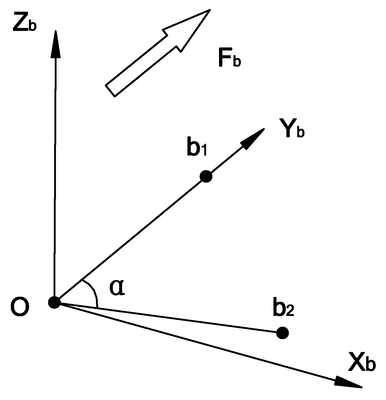
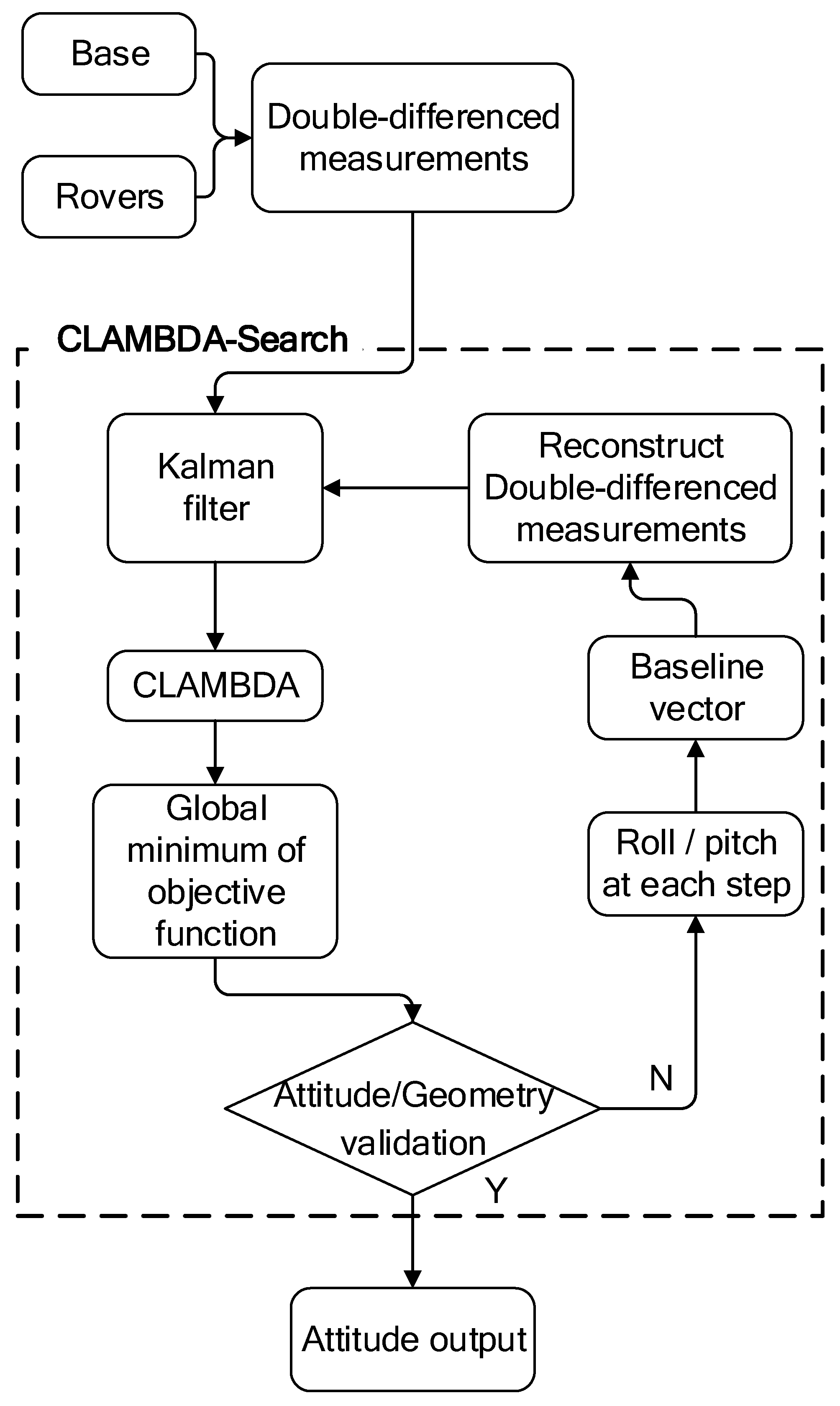
3. CLAMBDA-Search Model

Low-cost GNSS receivers have unstable and less-qualified pseudorange and carrier observations, in terms of less observation frequency, larger observation noise, and weak phase tracking capability. Therefore, the performance of low-cost receivers will face greater challenges when the signal is blocked. In urban environments, the signal block phenomenon occurs frequently, and the correspondent multipath errors are serious. Even if the signals are received by antennas that are very close to each other, and they may still have different observations, the ambiguity fixing success rate of multiple baselines is highly related to the environment. Therefore, this paper will combine the characteristics of vehicle attitude determination, taking into account geometric information, and improve the existing methods in the ambiguity domain and attitude domain, to obtain more reliable results.

3.1. An Improved Method for Single-Frequency Single-Epoch Attitude Determination

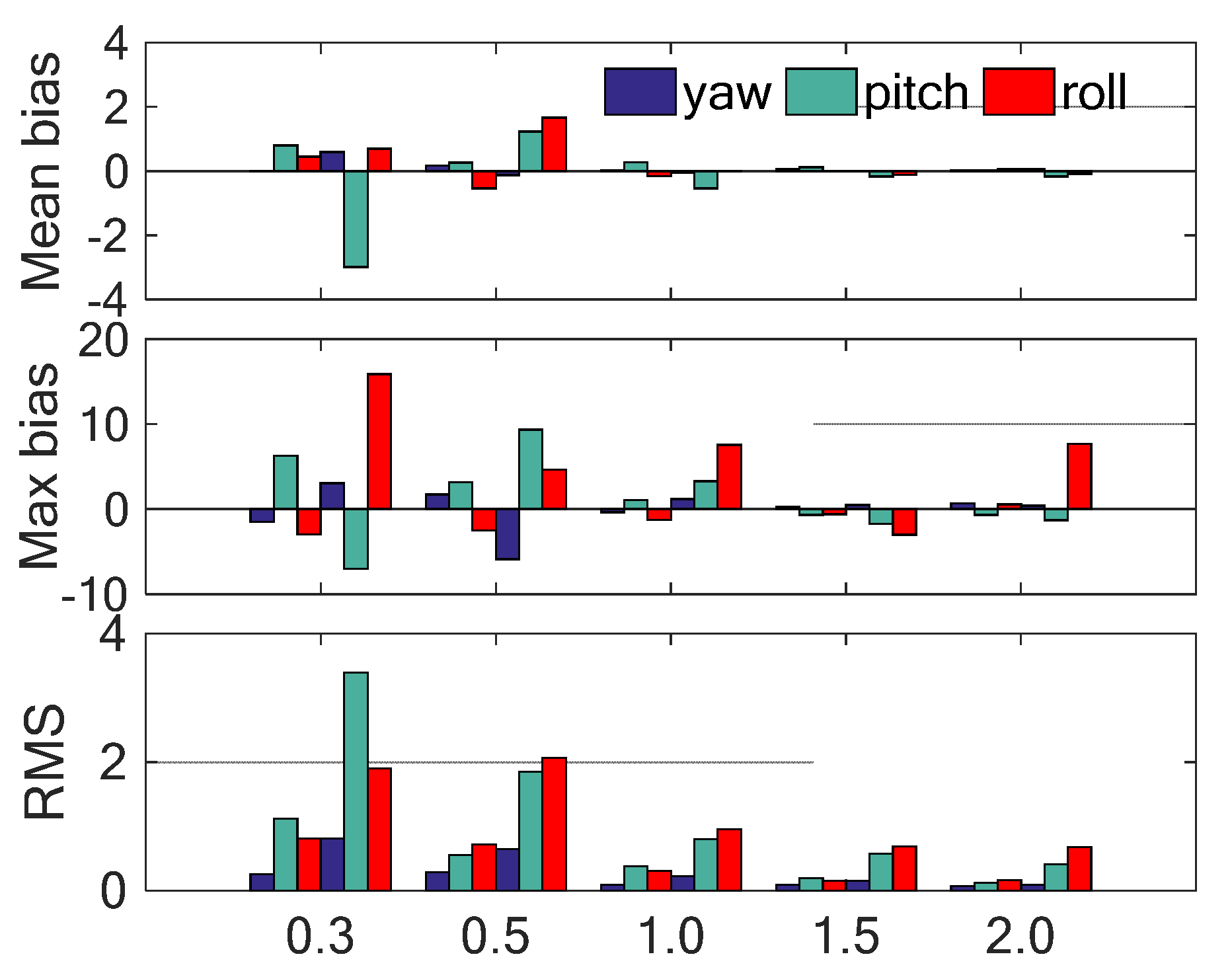
For vehicle three-antenna attitude determination applications, wrong ambiguity fixing is hard to avoid for one or two baselines with poor-quality data in the CLAMBDA method. In order to solve this problem and improve the applicability of low-cost receiver attitude determination, this paper proposes a Euler angle search and single degree of freedom in an unfixed direction method called CLAMBDA-search, which adopts the CLAMBDA method to fix the ambiguity and then the attitude parameters.

The three-antenna layout is shown in Figure 1, and wrong fixing of baseline two is taken as an example. When baseline one is correctly fixed, and baseline two cannot be fixed or incorrectly fixed, we can apply the method proposed in this study. However, when baseline one fails to fix, that is, when baseline two becomes the primary baseline, the angle determination method is slightly different. We will discuss this situation later. Here, baseline one is set as the primary baseline. Given the baseline vector, as follows:

$$\begin{array}{l}{\stackrel{⌣}{b}}_1^n=\left(e_1{n}_1{u}_1\right),{\hat{b}}_2^n=\left(e_2{n}_2{u}_2\right),\\ b_1^b=\left(0l_{1}0\right),b_2^b=\left(l_2\sin \alpha l_2\cos \alpha 0\right)\end{array}$$

(14)

where ${\stackrel{⌣}{b}}_1^n$ is the fixed vector of baseline one in the local frame, ${\hat{b}}_2^n$ is the float vector of baseline two; and $b_1^b$ and $b_2^b$ are the known coordinates in the carrier coordinate system, which can be obtained in advance by some other technologies such as total station, static GNSS continuous observation, etc.

According to the first two terms in (14), we can obtain the ambiguity-fixed yaw ($\stackrel{⌣}{\psi }$) and pitch ($\stackrel{⌣}{\theta }$), along with the ambiguity-float roll (${\hat{\gamma }}_0$). So far, we have obtained two ambiguity-fixed angles and one remaining unfixed angle. With these three angles, we construct an Euler angle $E_0=(\begin{array}{ccc}\stackrel{⌣}{\psi }& \stackrel{⌣}{\theta }& {\hat{\gamma }}_0\end{array})$. We set a searching region for the roll (${\hat{\gamma }}_0$) angle and carry out the searching process as follows:

$${\hat{\gamma }}_0,{\hat{\gamma }}_0-\eta ,{\hat{\gamma }}_0+\eta ,{\hat{\gamma }}_0-2\eta ,{\hat{\gamma }}_0+2\eta ,\cdots$$

(15)

where $\eta$ is the searching step. Obviously, the step size is a trade-off between searching accuracy and searching efficiency. We will discuss this topic in the next sub-section.

This searching strategy was proposed independently, by Schnorr and Euchner [34]. For any value in the searching region, the corresponding direction cosine matrix is represented as $C_b^n(k)$. Then, it is expressed as follows:

$${\stackrel{⌣}{b}}_2^n(k)=C_b^n(k)b_2^b$$

(16)

Substituting ${\stackrel{⌣}{b}}_2^n(k)$ into the observation equation, the observation equation can be expressed as follows:

$${\phi }_{DD}{}^2={\hat{N}}_{DD}{}^2+G{({\stackrel{⌣}{b}}_2^n(k))}^2{\stackrel{⌣}{b}}_2^n(k)+v_{DD}^{\phi }{}^2$$

(17)

where ${\phi }_{DD}{}^2$ is the double-differenced carrier phase observation; ${\hat{N}}_{DD}{}^2$ is the float ambiguity; $G{({\stackrel{⌣}{b}}_2^n(k))}^2$ is the construction matrix based on ${\stackrel{⌣}{b}}_2^n(k)$; and $v_{DD}^{\phi }{}^2$ is the residual vector. All the superscripts of two represent the second baseline of the corresponding part of the matrix. We can derive the sole fixed ambiguity ${\hat{N}}_{DD}{}^2$ whose error ${\delta }_{{\hat{N}}_{DD}{}^2}$ conforms to the same distribution of $v_{DD}^{\phi }{}^2$. Given the construction matrix $G{(b_2^n)}^2$ and the true value of the baseline vector $b_2^n$, we have the following:

$${\delta }_{{\hat{N}}_{DD}{}^2}=v_{DD}^{\phi }{}^2=G{(b_2^n)}^2{b}_2^n-G{({\stackrel{⌣}{b}}_2^n(k))}^2{\stackrel{⌣}{b}}_2^n(k)\to N\left(0,Q_{DD}^{\phi }{}^2\right)\mathrm{with}{\stackrel{⌣}{b}}_2^n(k)\to b_2^n(k)$$

(18)

where ${\stackrel{⌣}{\gamma }}_k\to \gamma$. If ${\stackrel{⌣}{\gamma }}_k$ is very close to its true value $\gamma$, we can assume that $v_{DD}^{\phi }{}^2$ is normally distributed, and so the ambiguity error ${\delta }_{{\hat{N}}_{DD}{}^2}$. Based on the covariance propagation law, we have the following:

$$Q_{{\hat{N}}_{DD}{}^2}={\sigma }_{{\phi }_{DD}}^2{\left[G^T{({\stackrel{⌣}{b}}_2^n(k))}^{2}G{({\stackrel{⌣}{b}}_2^n(k))}^2\right]}^{-1}$$

(19)

With the known conditions above, we can then conduct the standard CLAMBDA searching. The ambiguity-fixed baseline solution is that with the smallest ambiguity function.

$${\stackrel{⌣}{z}}_j^2=\arg \underset{z\in Z^{n2}}{\min }F\left(z|{\gamma }_j\right)$$

(20)

where, the ambiguity function takes the unknown attitude angle (which is is roll here) into account.

$$\underset{z\in Z^n}{\min }\left({‖\hat{z}-z‖}_{Q_{\stackrel{⌢}{z}}}^2+\underset{b\in R^3}{\min }H(z,b)+\frac{‖\stackrel{⌣}{\theta }-\hat{\theta }‖}{{\sigma }_{\theta }^2}\right)\mathrm{with}H(a,b)={‖\hat{b}\left(z\right)-b‖}_{Q_{\hat{z}}}^2+\frac{‖\stackrel{⌣}{\theta }-\hat{\theta }‖}{{\sigma }_{\theta }^2}+{\sigma }_l^{-2}(l-‖b‖)$$

(21)

The correct fixing result cannot always be available for most searched rolls in the region. Some approximate value of the roll angle, by just one or a few values, can yield normally distributed residuals, and then fix the correct ambiguity. In order to retrieve the closest solution to the roll angle, we can take the global minimum value of the ambiguity function, as follows:

$$j_0=\arg \underset{j}{\min }F\left({\stackrel{⌣}{z}}_j|{\gamma }_j\right),-N(z,\gamma )\le j\le N(z,\gamma )$$

(22)

where $N(z,\gamma )$ is the searching boundary, which affects the float roll angle and the searching efficiency. So far, we have got the new algorithm, and further discussion is needed.

The flowchart of the proposed CLAMBDA-search method is shown in Figure 2, and the corresponding procedures are as follows:

Step 1: use the code and phase observations to construct double-differenced measurements;

Step 2: apply the Kalman filter to estimate the multi-baseline unknown parameters;

Step 3: apply the CLAMBDA for the baseline without correctly fixed ambiguity, and record the current minimum of the fixed ambiguity objective function;

Step 4: Apply attitude and geometry validation (see validation section). If the conditions are satisfied or the searching procedure is done, output the results. If any of the condition is not satisfied, start roll or pitch searching, re-construct double-differenced measurements, and jump to step 2.

3.2. Error Analysis

Once the ambiguity is fixed by (16), we can get all the ambiguity solutions and the ambiguity-fixed baseline vector. According to the relationship between the baseline and the attitude angle in (13), the differential equation of the attitude angles and the covariance propagation law, the error expression of the attitude angle can be derived. Define the posterior baseline error as follows:

$${\sigma }_{{\stackrel{⌣}{b}}_1^n}=\left(\begin{array}{ccc}{\sigma }_{e_1}& {\sigma }_{n_1}& {\sigma }_{u_1}\end{array}\right){\sigma }_{{\stackrel{⌣}{b}}_2^n}=\left(\begin{array}{ccc}{\sigma }_{e_2}& {\sigma }_{n_2}& {\sigma }_{u_2}\end{array}\right)$$

(23)

Conduct a differential process to $\psi$ in (13), as follows:

$$\begin{array}{l}d\psi =-\frac{1}{1+{(e_1/n_1)}^2}\left(\frac{d{e}_1}{n_1}-\frac{e_1}{n_1{}^2}d{n}_1\right)=\frac{-n_{1}d{e}_1+e_{1}d{n}_1}{e_1{}^2+n_1{}^2}\\ d\psi =\frac{-\cos \psi d{e}_1+\sin \psi d{n}_1}{l_1\cos \theta }\end{array}$$

(24)

If one ignores the covariance between the baseline components, the heading angle error is expressed as follows:

$${\sigma }_{\psi }=\frac{\sqrt{{\sigma }_e^2{\cos }^2\psi +{\sigma }_n^{2}si{n}^2\psi }}{l_1\cos \theta }$$

(25)

Similarly, the error expressions of the pitch and roll angle are described as follows:

$$\begin{array}{l}{\sigma }_{\theta }=\frac{\sqrt{{\sin }^2\psi \cdot {\sin }^2\theta \cdot {\sigma }_{e_1}^2+{\cos }^2\psi \cdot {\sin }^2\theta \cdot {\sigma }_{n_1}^2+{\cos }^2\theta \cdot {\sigma }_{u_1}^2}}{l_1}\\ {\sigma }_{\gamma }=\frac{\sqrt{{\sin }^2\gamma \cdot {\sigma }_{{e^{\prime }}_2}^2+{\cos }^2\gamma \cdot {\sigma }_{{u^{\prime }}_2}^2}}{l_2\cdot \sin \alpha }\end{array}$$

(26)

where the following is applied:

$$\begin{array}{l}{\sigma }_{{e^{\prime }}_2}^2={\cos }^2\psi \cdot {\sigma }_{e_2}^2+{\sin }^2\psi \cdot {\sigma }_{n_2}^2\\ {\sigma }_{{u^{\prime }}_2}^2={\sin }^2\psi \cdot {\sin }^2\theta \cdot {\sigma }_{e_2}^2+{\cos }^2\psi \cdot {\sin }^2\theta \cdot {\sigma }_{n_2}^2+{\cos }^2\theta \cdot {\sigma }_{n_2}^2\end{array}$$

(27)

It can be seen, from (25)–(27), that the accuracies of the heading angle and pitch angle are only related to the primary baseline (baseline one). The longer the baseline length is, the smaller the error is. On the other hand, the roll angle is dependent on the baseline length, as well as the baseline geometry. The long baseline length, and the closeness of the two-baseline angle to 90°, yield the smaller error.

In the CLAMBDA-search method, one degree of freedom exists in the roll angle direction, when baseline one is fixed. Since the distance between the searched solution and its true value is very far from the distance between the receiver and the satellite, we can assume $G{(b_2^n)}^2\approx G{({\stackrel{⌣}{b}}_2^n(k))}^2$. Then, for a certain value $E(k)=(\begin{array}{ccc}\stackrel{⌣}{\psi }& \stackrel{⌣}{\theta }& {\hat{\gamma }}_k\end{array})$ within the searching region, we have the following:

$${\delta }_{{\hat{N}}_{DD}{}^2}=G{(b_2^n)}^2{b}_2^n-G{({\stackrel{⌣}{b}}_2^n(k))}^2{\stackrel{⌣}{b}}_2^n(k)\approx G{({\stackrel{⌣}{b}}_2^n(k))}^2(b_2^n-{\stackrel{⌣}{b}}_2^n(k))$$

(28)

The baseline coordinates can be expressed in the form of the baseline length and the attitude angle, as follows:

$$b_2^n=C_b^{n1}{b}_2^b=C_b^{n1}\left[\begin{array}{c}{l}_2\sin \alpha \\ l_2\cos \alpha \\ 0\end{array}\right]$$

(29)

Then, Equation (28) can be expressed as follows:

$${\delta }_{{\hat{N}}_{DD}{}^2}\approx G{({\stackrel{⌣}{b}}_2^n(k))}^2(b_2^n-{\stackrel{⌣}{b}}_2^n(k))\approx l_{2}G{({\stackrel{⌣}{b}}_2^n(k))}^2\left[\begin{array}{c}\cos \gamma -\cos {\gamma }_k\\ 0\\ -\sin \gamma +\sin {\gamma }_k\end{array}\right]$$

(30)

It is clear, from (30), that the distribution of ambiguity error is dependent on the baseline length. The longer the baseline length is, the greater the difference between the roll angle and its true value is. Obviously, a small step size has a large possibility to reach the true value, and then easy ambiguity fixing. However, a small step size means a lot of computing time. Therefore, we will design several experiments with various baseline lengths and step sizes, to seek a more suitable searching method.

3.3. Validation

As the CLAMBDA method changes the ambiguity objective function, the ambiguity vector does not conform to the ${\chi }^2$ distribution. That means the general ratio test cannot be used to verify the correctness of the ambiguity fixing solution. For a single baseline, the baseline length can be used as an ambiguity validation means. As for the multiple-baseline case, the redundant geometric condition and the DCM projection can be adopted for the ambiguity validation.

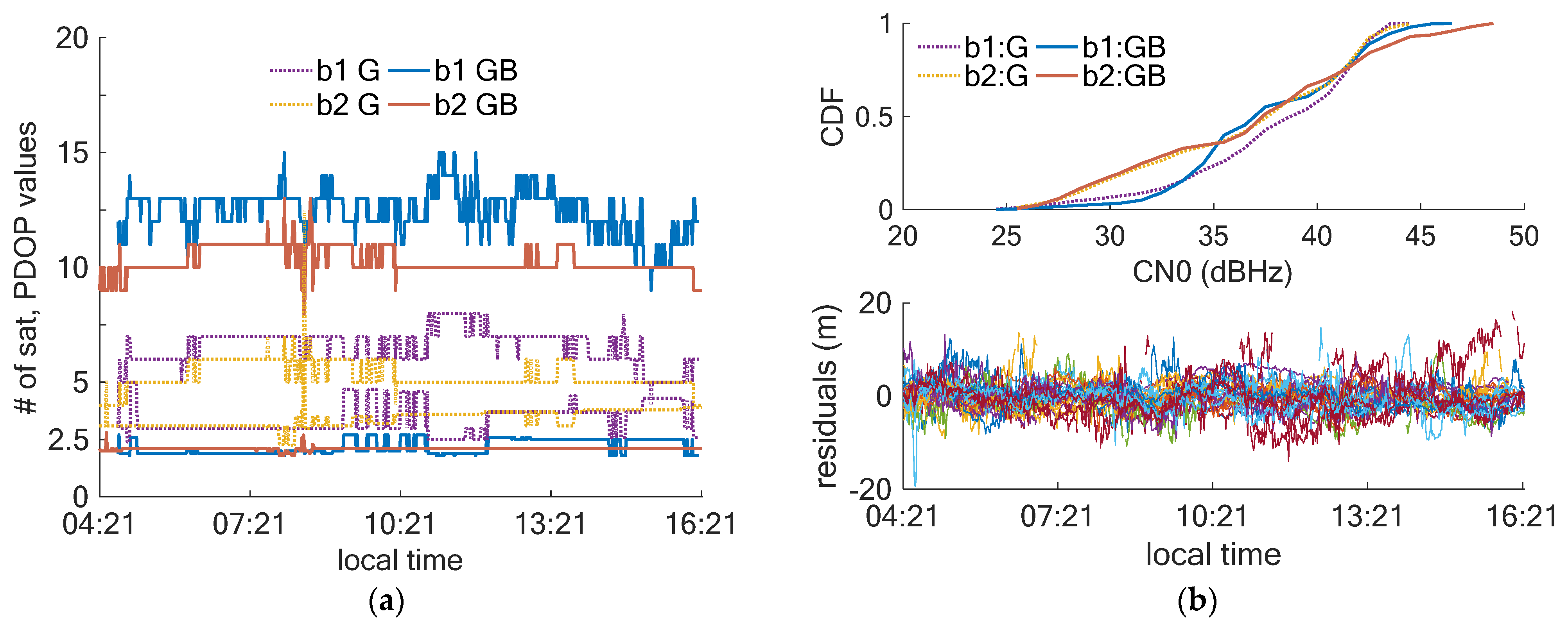
3.3.1. Baseline Length Check

For the minimum requirement of the ambiguity objective function, the baseline obtained by CLAMBDA should conform to the known baseline length condition. However, due to wrong data and excessive searching time, a satisfactory solution may not be obtained within a specified searching duration. The threshold is set as 0.03 m in this paper.

3.3.2. Geometric Condition Check

In the kinematic scenario, the antenna is fixed on the vehicle roof so it can be considered as a rigid body. Therefore, the angle between the two baselines in the local frame should meet the condition.

$${\stackrel{⌣}{b}}_1^n·{\stackrel{⌣}{b}}_2^n-‖b_1^b‖‖b_2^b‖\cos \alpha <{\tau }_{geo}$$

(31)

where ${\tau }_{geo}$ is the empirical threshold, set as 0.2 in this paper.

3.3.3. Attitude Angle Check

If any given ${\gamma }_k$ is close to its true value $\gamma$, the calculated value ${{\gamma }^{\prime }}_k$ with the fixed ambiguity should also be close to ${\gamma }_k$. Then, we can check by using the following:

$$\left|{{\gamma }^{\prime }}_k-{\gamma }_k\right|<{\tau }_{att}$$

(32)

3.3.4. Maximum Pitch and Roll Angle Check

The pitch and roll angle are often within a certain range in ground vehicle applications. So, the coordinate difference between the two fixed baseline vectors in the u direction should meet this condition. In this search, we set the maximum pitch and roll to 45 degrees.

3.4. Additional Discussion

We have discussed the necessary concepts of the proposed method in the previous sub-section, with baseline one as the primary baseline (when baseline one is correctly fixed). However, the procedure is slightly different when baseline two becomes the primary baseline. Due to the definition of DCM, we have to adopt another Euler angle definition approach when baseline two is treated as the primary baseline. The rotation of the rigid body is related to the direction and the order, which will probably cause misunderstanding. Because the baseline installation angle in the body frame cannot be guaranteed to be completely orthogonal, switching the primary baseline also means a change in the vehicle coordinate system, which would further cause a difference in the attitude angle. This sub-section will discuss these problems. DCM, with the Euler angle derived by baseline one as the primary baseline, is defined as follows:

$$C_b^{n1}=\left[\begin{array}{ccc}\mathrm{c}\psi \mathrm{c}\gamma -\mathrm{s}\psi \mathrm{s}\theta \mathrm{s}\gamma & -\mathrm{s}\psi \mathrm{c}\theta & \mathrm{c}\psi \mathrm{s}\gamma +\mathrm{s}\psi \mathrm{s}\theta \mathrm{c}\gamma \\ \mathrm{s}\psi \mathrm{c}\gamma +\mathrm{c}\psi \mathrm{s}\theta \mathrm{s}\gamma & \mathrm{c}\psi \mathrm{c}\theta & \mathrm{s}\psi \mathrm{s}\gamma -\mathrm{c}\psi \mathrm{s}\theta \mathrm{c}\gamma \\ -\mathrm{c}\theta \mathrm{s}\gamma & \mathrm{s}\theta & \mathrm{c}\theta \mathrm{c}\gamma \end{array}\right]$$

(33)

where c is the cosine function and s is the sine function.

However, in order to ensure that searching can be performed when baseline two is fixed, DCM, with the Euler angle derived by baseline two as the primary baseline, is as follows:

$$C_b^{n2}=\left[\begin{array}{ccc}\mathrm{c}\psi \mathrm{c}\gamma & -\mathrm{s}\psi \mathrm{c}\theta +\mathrm{s}\psi \mathrm{s}\theta \mathrm{s}\gamma & \mathrm{s}\psi \mathrm{s}\theta +\mathrm{c}\psi \mathrm{c}\theta \mathrm{s}\gamma \\ \mathrm{s}\psi \mathrm{c}\gamma & \mathrm{c}\psi \mathrm{c}\theta +\mathrm{s}\psi \mathrm{s}\theta \mathrm{s}\gamma & -\mathrm{c}\psi \mathrm{s}\theta +\mathrm{s}\psi \mathrm{c}\theta \mathrm{s}\gamma \\ -\mathrm{s}\gamma & \mathrm{c}\psi \mathrm{s}\theta & \mathrm{c}\psi \mathrm{c}\theta \end{array}\right]$$

(34)

Although these two forms are not identical, their algebraic values are exactly the same. Therefore, we directly give the formula for calculating the Euler angle by the direct method as follows:

$$\begin{array}{l}\psi =\arctan \left(\frac{n_2}{e_2}\right)\\ \gamma =-\arctan \left(\frac{u_2}{\sqrt{e_2^2+n_2^2}}\right)\\ \theta =-\arctan \left(\frac{\sin \gamma \cos \psi e_1+\sin \gamma \sin \psi n_1+\cos \gamma u_1}{-\sin \psi e_1+\cos \psi n_1}\right)\end{array}$$

(35)

The CLAMBDA-search process afterwards is exactly the same. However, the attitude angle, with baseline two as the primary baseline, will face the problem of inconsistent coordinate systems. Fortunately, since the baseline is fixed, we only need to re-calculate the attitude angle, using baseline one as the primary baseline. For the antenna’s non-orthogonal error, the vehicle coordinates in the body frame are as follows:

$$b_1^b(1)=\left[\begin{array}{c}0\\ l_1\\ 0\end{array}\right],b_2^b(1)=\left[\begin{array}{c}{l}_2\sin \alpha \\ l_2\cos \alpha \\ 0\end{array}\right],b_1^b(2)=\left[\begin{array}{c}{l}_2\cos \alpha \\ l_2\sin \alpha \\ 0\end{array}\right],b_2^b(2)=\left[\begin{array}{c}{l}_2\\ 0\\ 0\end{array}\right]$$

(36)

where the digits in brackets represent the primary baseline. However, the b-system coordinates and the corresponding attitude angles will be inconsistent with different antenna layouts. The principle is to convert them to a unified right-handed coordinate system. Therefore, for the definition of body frame as RFU, the angle $\alpha$ between the baselines is defined as follows:

• $b_1$ is the primary baseline. Starting from $b_1$, turn to $b_2$ in the clockwise direction. If $b_1$ is negative, then $\alpha =\alpha +\pi$;
• $b_2$ is the primary baseline. Starting from $b_2$, turn to $b_1$ in the anti-clockwise direction. If $b_2$ is negative, then $\alpha =\alpha +\pi$.

In the meantime, the conversion of $\theta$ and $\gamma$ is required when converting to the positive right-handed coordinate system if the negative axis is defined.

For different baseline configurations, we must use the vehicle coordinate system, the Euler angle definition and DCM in a consistent manner. Otherwise, it will cause unpredictable consequences because of the definition of the Euler angle and coordinate system. So far, the problems of different vehicle coordinate systems, different attitude angle definitions, and the antenna’s non-orthogonal errors have been successfully resolved.

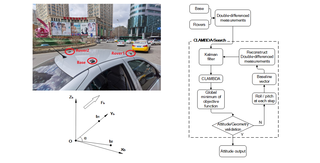
4. Experiments and Results

In this part, several independent experiments will be carried out to test the performance of the CLAMBDA-search method with real-world data. First, we introduce a static experiment and its results. Then, we will show a dynamic one. The antenna coordinates in the body frame are obtained from the GNSS static results in the paper.

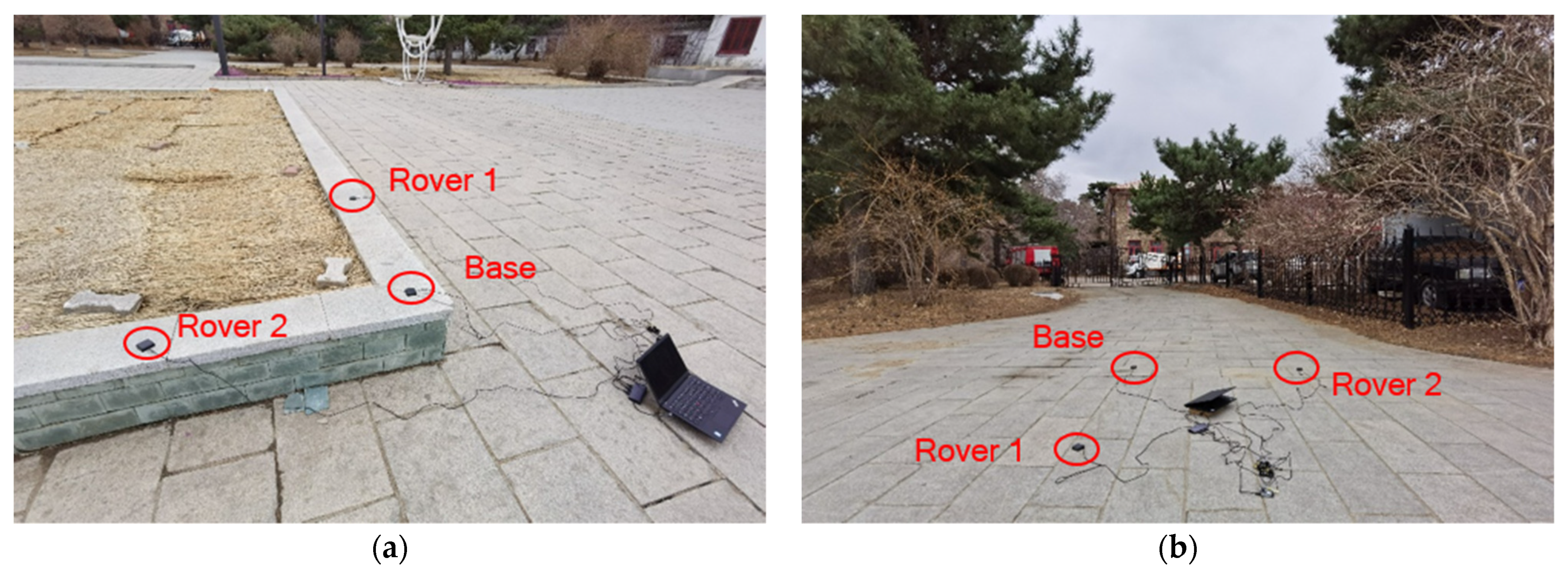
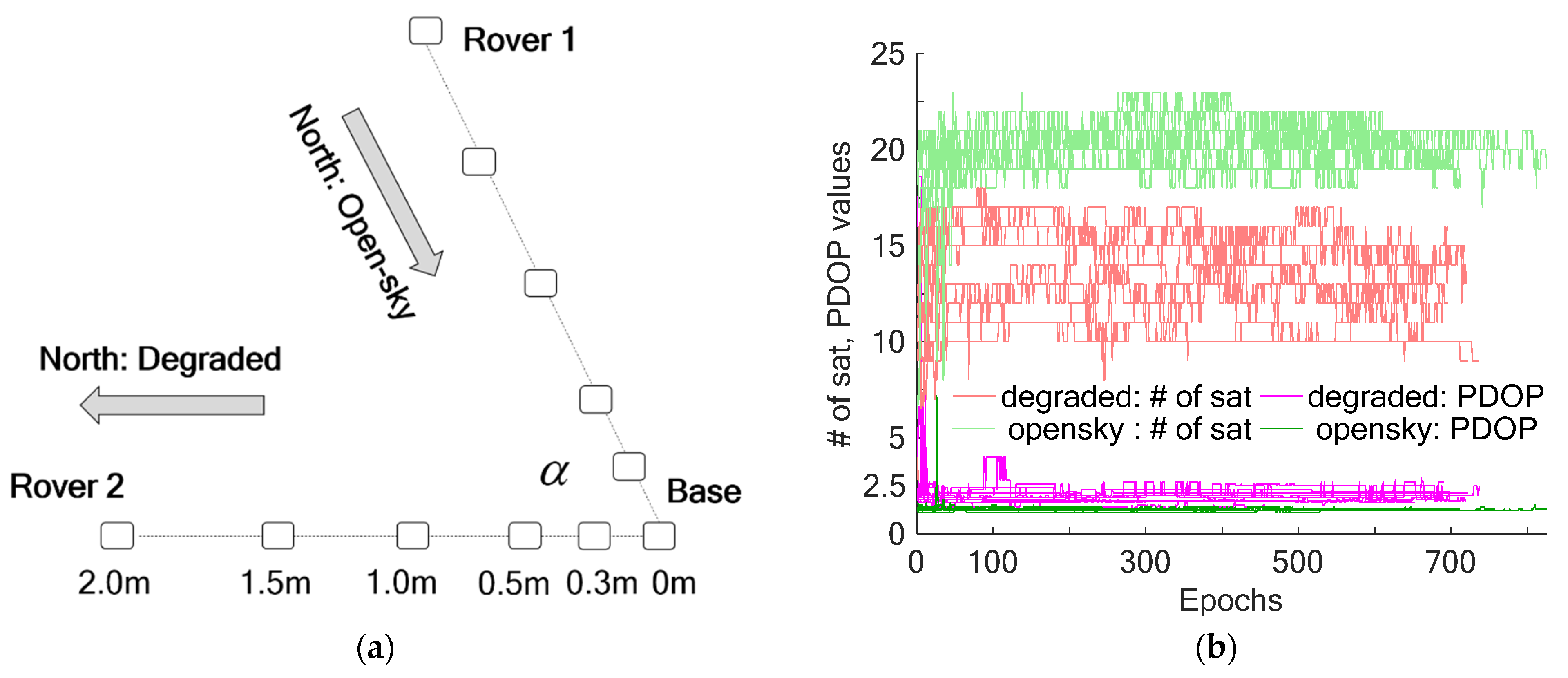
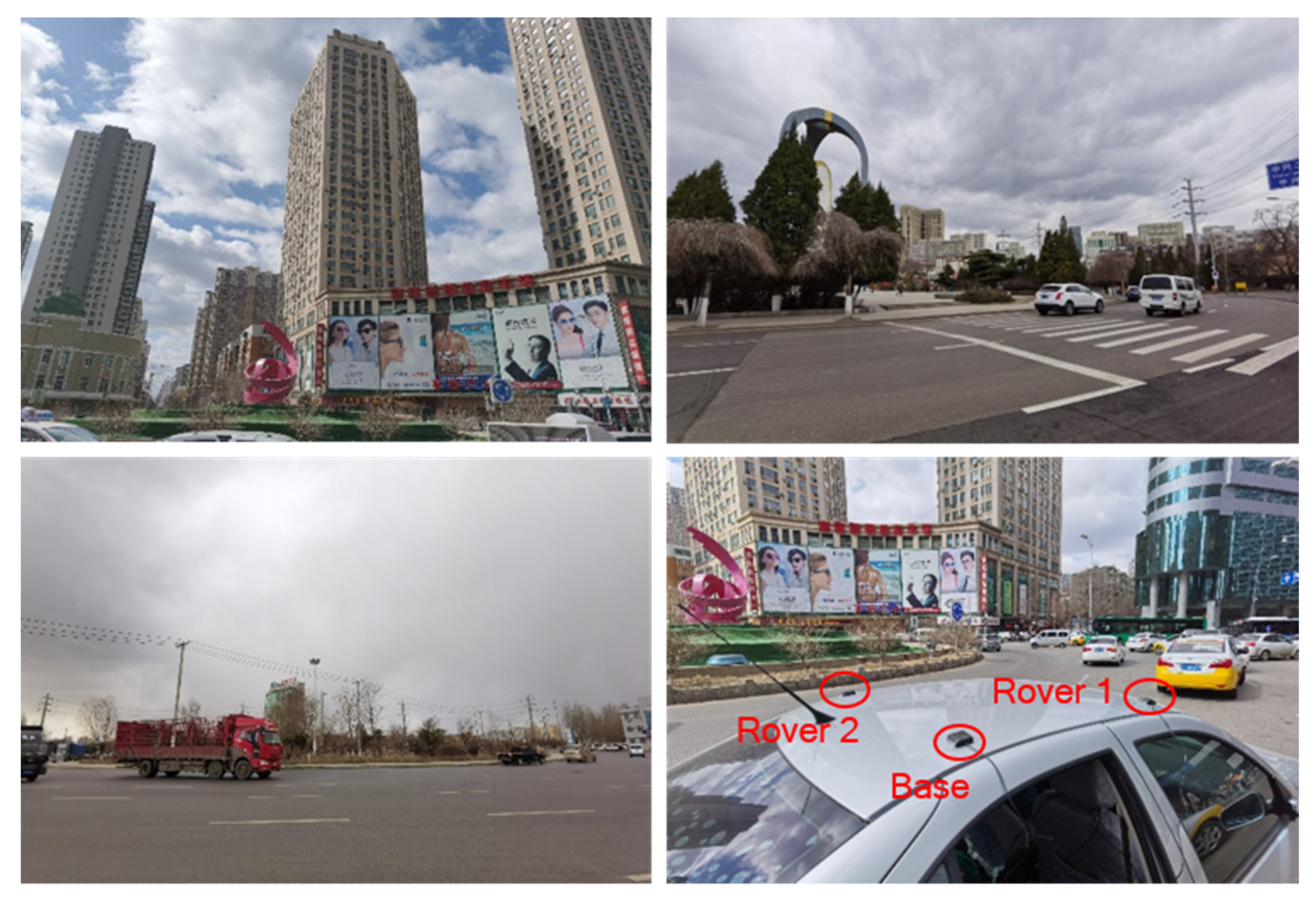
4.1. Static Experiment

In order to assess the proposed CLAMBDA-search method with low-cost receivers in complex environments, this study utilizes three Ublox M8T receivers and a patch antenna to form a three-baseline layout. We conducted five tests with baseline lengths of 0.3, 0.5, 1.0, 1.5 and 2.0 m in open and blocked environments. GNSS data collection was carried out near the Huangtaiji Mausoleum in Huanggu District, Shenyang, China.

Figure 3 shows the antenna layout for the open-sky and degraded environment, respectively. In the open-sky environment, the antenna is placed at the corner of a flower bed, whereas it is placed under two tall trees in the degraded environment. The GNSS data collection frequency is 1 Hz. The elevation cutoff angle is set to 10°. Each test lasts for about 12 min in the morning of 8 March 2020.

Figure 4 demonstrates the antenna setup in the two tests. Base, rover 1, and rover 2 represent three Ublox receivers. ${\stackrel{\rightharpoonup }{b}}_1=\stackrel{\rightharpoonup }{BaseRover1},{\stackrel{\rightharpoonup }{b}}_2=\stackrel{\rightharpoonup }{BaseRover2}$. $\alpha$ is the angle between the two baselines. Figure 4 also depicts the number of tracked GPS and BDS satellites and the correspondent PDOP value. The light-green and dark-green line represents the open-sky scenario, while the red and magenta line represents the degraded scenario. We can find that the satellite number is higher with dual satellite systems, and the PDOP value is mostly below 2.5. The active satellite number changes occur in the beginning. This phenomenon is caused by the receiver cold startup on satellite tracking. All the experimental data are solved using LAMBDA (approach I), CLAMBDA (approach II), MCLAMBDA (approach III) and CLAMBDA-search (approach IV) in sequence. The ratio of LAMBDA ambiguity validation is set as three. The baseline variance of CLAMBDA is set as 0.05 m. The step size of CLAMBDA-search is set as 2.5°. We use the average as a reference value, and the ambiguity fixing success rate and correct fixed rate are expressed as follows:

$$P_{s_E}=\frac{\#\mathrm{of}\mathrm{fixed}\mathrm{epochs}}{\mathrm{total}\#\mathrm{of}\mathrm{epochs}},P_{s_E|c}=\frac{\#\mathrm{of}\mathrm{correctly}\mathrm{fixed}\mathrm{epochs}}{\mathrm{total}\#\mathrm{of}\mathrm{epochs}}$$

(37)

Table 1. SFSE (single-frequency single epoch) ambiguity fixing rate and correct fixed rate of various designed and actual baseline lengths (GPS-only observations, open sky), LAMBDA (approach I), CLAMBDA (approach II), MCLAMBDA (approach III) and CLAMBDA-search (approach IV). The column in the table is the designed baseline length.

Method		0.3	0.5	1.0	1.5	2.0
I	b1	1.9(0.0)	2.8(0.2)	2.0(0.4)	3.8(3.0)	2.9(1.4)
	b2	3.4(0.1)	2.8(0.1)	1.8(0.0)	6.2(4.5)	2.9(0.5)
II	b1	66.9(51.0)	61.7(58.4)	74.6(68.8)	93.1(91.4)	73.8(71.1)
	b2	68.1(54.8)	42.8(42.2)	77.6(68.8)	86.8(78.4)	75.9(73.3)
III	b1	55.3(55.3)	50.3(50.3)	79.1(79.1)	83.0(83.0)	54.5(54.5)
	b2	57.0(57.0)	49.5(49.5)	78.6(78.6)	84.6(84.6)	54.5(54.5)
IV	b1	53.7(53.3)	67.0(66.8)	81.6(81.6)	93.8(93.4)	88.7(86.2)
	b2	61.0(60.0)	56.0(55.8)	82.6(82.3)	94.7(94.7)	92.4(92.3)

,

Table 2. SFSE ambiguity fixing rate and correct fixed rate of various designed and actual baseline lengths (GPS + BDS observations, open sky).

Method		0.3	0.5	1.0	1.5	2.0
I	b1	97.3(97.3)	97.5(97.5)	93.0(93.0)	96.7(96.7)	95.9(95.9)
	b2	98.4(98.4)	91.6(91.6)	99.3(99.3)	95.5(95.5)	98.1(98.1)
II	b1	100(100)	100(100)	100(100)	99.9(99.9)	99.7(99.5)
	b2	100(100)	99.7(99.7)	100(100)	100(100)	100(100)
III	b1	99.5(99.5)	99.1(99.1)	100(100)	99.8(99.8)	99.4(99.4)
	b2	99.5(99.5)	99.2(99.2)	100(100)	100(100)	99.4(99.4)
IV	b1	100(100)	100(100)	100(100)	99.9(99.9)	99.7(99.7)
	b2	100(100)	100(100)	100(100)	100(100)	100(100)

,

Table 3. SFSE ambiguity fixing rate and correct fixed rate of various designed and actual baseline lengths (GPS-only observations, degraded).

Method		0.3	0.5	1.0	1.5	2.0
I	b1	4.9(0.0)	4.5(0.6)	4.5(0.0)	0.0(0.0)	4.9(0.4)
	b2	4.9(0.0)	8.2(1.7)	5.8(0.0)	0.0(0.0)	10.3(0.0)
II	b1	29.6(28.5)	52.7(45.3)	51.0(38.3)	47.8(4.0)	51.3(22.1)
	b2	50.3(46.5)	56.8(50.0)	41.7(21.7)	53.1(10.1)	55.4(0.5)
III	b1	28.3(28.3)	29.4(29.4)	14.8(14.8)	0.0(0.0)	4.9(4.9)
	b2	27.5(27.5)	28.9(28.9)	16.4(16.4)	0.0(0.0)	0.1(0.1)
IV	b1	46.2(45.3)	57.7(57.6)	42.4(42.0)	16.1(6.3)	27.2(25.0)
	b2	49.0(49.0)	54.4(54.2)	31.6(30.8)	16.1(11.8)	10.0(5.8)

and

Table 4. SFSE ambiguity fixing rate and correct fixed rate of various designed and actual baseline lengths (GPS + BDS observations, degraded).

Method		0.3	0.5	1.0	1.5	2.0
I	b1	63.0(63.0)	12.4(11.2)	44.9(44.4)	0.0(0.0)	19.3(19.3)
	b2	82.9(82.9)	9.7(0.0)	4.8(4.8)	0.0(0.0)	1.1(0.0)
II	b1	100(100)	99.3(98.3)	97.9(97.2)	75.0(73.3)	97.4(97.4)
	b2	99.4(99.2)	98.9(98.7)	71.6(67.9)	71.2(57.5)	51.2(21.3)
III	b1	98.7(98.7)	98.6(98.6)	81.8(81.8)	44.1(44.1)	37.2(37.2)
	b2	98.7(98.7)	96.9(96.9)	78.6(78.6)	37.1(36.1)	26.9(26.1)
IV	b1	100(100)	99.3(98.9)	97.9(97.9)	81.9(81.9)	99.3(99.3)
	b2	99.4(99.4)	98.9(98.7)	78.2(78.0)	73.6(71.1)	56.7(56.0)

show all the results calculated by the four methods represented in $P_{s_E}(P_{s_E|c})$, with the best solution in bold. The meaning of the rows and columns in the tables is the same. It is worth noting that since the checks in chapter validation are common in attitude determination, this method is also used in the MCLAMBDA in this article.

As for the open-sky environment, i.e., Table 1 and Table 2, the LAMBDA method has a poor fixing performance in the case of the low-cost receiver SFSE. It is difficult to fix the ambiguity with GPS-only observations, and this may be due to the SFSE solution strategy and fewer satellites. The GPS + BDS solution only obtains satisfactory results in group 1.0 m. This is due to the large pseudorange observation noise of the low-range receiver. The CLAMBDA method with the GPS-only observations does not perform as well as that with the dual-system observations. There is a lot of wrong fixing in the single-system solution. When dual systems are used, the wrong fixing rate is significantly reduced. However, the CLAMBDA method does not show obvious ambiguity fixing improvements with the different baseline lengths. This finding is consistent with that in Teunissen [28]. The MCLAMBDA method shows reliable results. At last, the CLAMBDA-search method proposed in this paper shows the best performance in both the single-system and dual-system scenarios for all baseline lengths. More importantly, there is no wrong fixing for the dual-system test. This is a remarkable feature for navigation applications with low-cost receivers.

As for the degraded environment, i.e., Table 3 and Table 4, the LAMBDA method still shows the worst performance. Similarly, the CLAMBDA method has a lot of wrong fixing results, especially in the single-system solution. The MCLAMBDA method still shows reliable results, but the number of solutions is insufficient. This may be caused by the limitation of requests for the same observations between baselines. The CLAMBDA-search method performs the best in both the single-system and multi-system solutions, in terms of the highest correct fixing rate. Even for the worst 1.5 m group, CLAMBDA-search can still maintain an 81.90% and 73.55% ambiguity fixing rate, and 100.00% and 96.60% correct fixed rate, which are higher than the CLAMBDA method by 11.76% and 23.61%, respectively. Obviously, the CLAMBDA-search method proposed in this paper is more resistant to the multipath effect than both CLAMBDA and MCLAMBDA in the degraded environment, and it has better robustness.

Based on Table 2 and Table 3, Figure 5 summarizes the average error, maximum error and RMS of the attitude angles derived by the CLAMBDA-search method. It can be found that since this study uses the direct approach to calculate the attitude angle, the correspondent attitude error conforms to the inverse proportional relationship with the baseline length. The longer the baseline length is, the smaller the attitude error is. The best attitude accuracy ${\sigma }_{\psi }=0.07°,{\sigma }_{\theta }=0.12°,{\sigma }_{\gamma }=0.16°$ occurs for the group 2.0 m.

It can be preliminarily concluded that the LAMBDA method has the worst performance for the low-cost receiver SFSE, which is not recommended. The CLAMBDA method cannot eliminate wrong fixing, due to the absence of verification conditions. The MCLAMBDA method could give reliable results, but the number of solutions is small when the observation quality is not so good. The CLAMBDA-search method proposed in this study has the advantages of a high fixing rate, fewer errors, and strong robustness, and thus is more suitable for land applications in complex environments.

For the worst data set, group 1.5 m in the degraded environment, the time series of the satellite number, PDOP values, C/N0 values and residuals are shown in Figure 6. Figure 6 shows the number of satellites and PDOP values of both the GPS and GPS/BDS solutions. For baseline one, the blue line is the dual-system solution and the purple dotted line is the single-system solution. For baseline two, the red line is the dual-system solution and the yellow dotted line is the single-system solution. From Figure 6—bottom panel—it can be found that for the baseline one, GPS has a better carrier-to-noise ratio than BDS. For GPS, the C/N0 of the 50% observations are greater than 38 dBHz, whereas the 50% BDS observations are just greater than 36 dBHz. As for baseline two, the carrier-to-noise ratios between GPS and BDS are similar to each other, i.e., the 50% observations are greater than 37 dBHz. Figure 6—bottom panel—also shows the observation residuals that indicate a strong multipath effect. That can explain why the SFSE’s LAMBDA cannot fix ambiguities.

Table 5. GPS/BDS attitude solution of group 1.5 m in degraded environments.

	Euler Success Rate (Correctly Fixed) [%]	$\mathit{\delta }\overline{\mathit{\psi }}({\mathit{\sigma }}_{\mathit{\delta }\overline{\mathit{\psi }}})[°]$	$\mathit{\delta }\overline{\mathit{\theta }}({\mathit{\sigma }}_{\mathit{\delta }\overline{\mathit{\theta }}})[°]$	$\mathit{\delta }\overline{\mathit{\gamma }}({\mathit{\sigma }}_{\mathit{\delta }\overline{\mathit{\gamma }}})[°]$
LAMBDA	0.0 (0.0)	NaN	NaN	NaN
CLAMBDA	55.3 (43.1)	3.14 (21.80)	−0.16 (3.41)	1.78 (20.13)
MCLAMBDA	36.9 (36.8)	−0.26 (−0.29)	0.22 (0.53)	−0.17 (−0.16)
CLAMBDA-search	68.4 (67.4)	−0.00 (0.15)	−0.17 (0.57)	−0.11 (0.68)

show the Euler angle success rate, Euler angle accuracy, and their average error and accuracy calculated by three methods. The Euler angle success rate is defined as the epoch when baseline one and two can both be fixed. The Euler angle accuracy rate is defined as the epoch when baseline one and two are both correctly fixed. Table 5 also shows that the dual-system attitude error of the CLAMBDA method is also unacceptable. The MCLAMBDA method has a small attitude error, but lower Euler success rate. However, the dual-system attitude error of the proposed CLAMBDA-search method is only 0.15°, 0.57°, 0.68°, which proves its outperformance over the other three methods.

Note that we cannot ignore the computational complexity for all the ambiguity searching algorithms.

Table 6. Calculation time [ms] for each test in the degraded environment.

Baseline Length	CLAMBDA	MCLAMBDA	CLAMBDA-Search 5°	CLAMBDA-Search 2.5°
0.3	0.71	57.01	52.63	107.19
0.5	0.72	67.81	65.09	111.58
1.0	0.73	154.79	71.95	140.93
1.5	1.34	315.64	85.14	161.82
2.0	0.74	472.12	93.34	188.47

shows the calculation time for each test. It should be noted that the maximum number of search times of method I/II/III is set to 10,000, and MCLAMBDA is set to 200,000 in this article. The calculation time consumed by each method only counts the searched results. For epochs that cannot be searched, each epoch ends with maximum number of search times. The elapsed times are measured at every epoch using C functions “QueryPerformanceCounter()” at a PC with Intel^® Core(TM) i7-7500 CPU @ 2.70 GHz and 8192 MB RAM.

As shown in Table 6, the searching time of the CLAMBDA method increases with the ascending baseline length, except for the 1.5 m baseline. The 1.5 m baseline requires a much longer searching time, due to poor observation conditions and the resultant unrealistic observation model. As for the MCLAMBDA method, it takes the longest time, except for CLAMBDA-search with $\eta =2.5°$. In fact, for all the unfixed epochs of the MCLAMBDA method, it ends up with 200,000 times searching for ambiguities, the total time of this method is very long. For the CLAMBDA-search method, the searching time of $\eta =5°$ is about one-half of $\eta =2.5°$. With the ascending baseline length, the searching time also increases. In fact, the actual data are often disturbed by the changing multipath as the baseline length increases. Thus, the success rates may decrease [33]. Another possible reason is that the increasing baseline length enlarges the ambiguity candidate regions, which makes the searching more time consuming. As the step size decreases, the Euler angle success rate continues to increase, as shown in

Table 7. Euler success rate with various steps for group 1.5 m in degraded environments.

Partition Accuracy [°]	Euler Success Rate (Correctly Fixed) [%]	$\mathit{\delta }\overline{\mathit{\psi }}({\mathit{\sigma }}_{\mathit{\delta }\overline{\mathit{\psi }}})[°]$	$\mathit{\delta }\overline{\mathit{\theta }}({\mathit{\sigma }}_{\mathit{\delta }\overline{\mathit{\theta }}})[°]$	$\mathit{\delta }\overline{\mathit{\gamma }}({\mathit{\sigma }}_{\mathit{\delta }\overline{\mathit{\gamma }}})[°]$	Mean Computing Time (ms)
1.25	69.7 (68.4)	−0.00 (0.15)	−0.17 (0.57)	0.11 (0.68)	330.18
2.5	68.4 (67.4)	−0.00 (0.15)	−0.17 (0.57)	−0.11 (0.68)	161.82
5	68.0 (67.0)	−0.00 (0.15)	−0.17 (0.58)	0.011 (0.68)	85.14
10	66.7 (65.7)	0.00 (0.15)	−0.16 (0.57)	−0.11 (0.69)	40.63
20	61.1 (60.1)	−0.00 (0.15)	−0.15 (0.57)	−0.13 (0.70)	20.80

. Equation (25) shows that the correct attitude angle will bring a more accurate ambiguity model, which is consistent with the experimental results. However, because the direct method is used for the attitude calculation, various step sizes do not affect the error characteristics. This can be attributed to the fact that the method performance is related to the baseline length. The average computing time is just 330 ms when $\eta =1.25°$, the same order of magnitude as the MCLAMBDA method, with better results at the same time. That means our method takes moderate computing burden and yields high efficiency. Meanwhile, we can customize the step $\eta$ to meet the need of the specific environment.

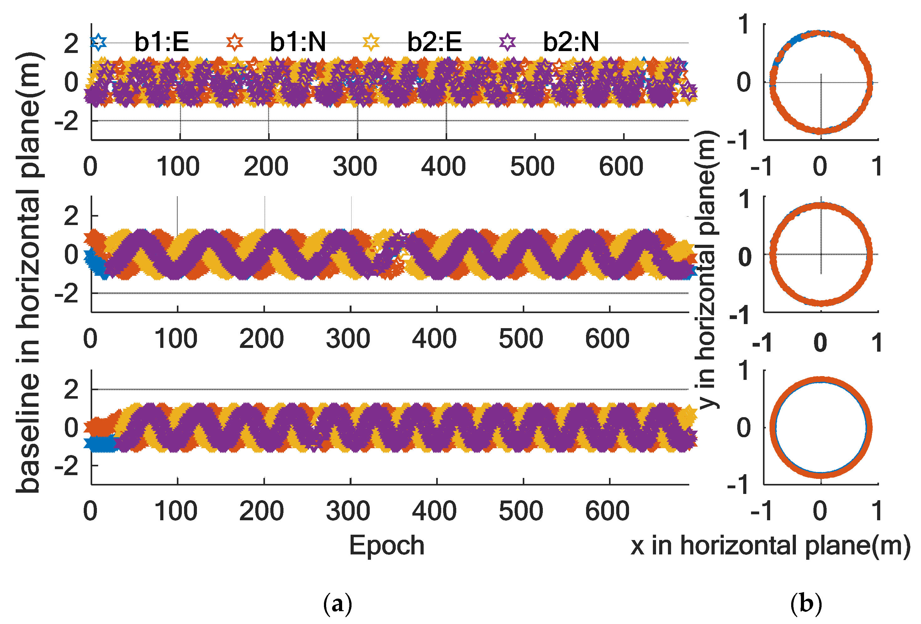
4.2. Dynamic Experiment

In this sub-section, we demonstrate the performance of the proposed CLAMBDA-search method for a moving vehicle. The data are collected at the interval of 1 Hz and with a 10° elevation cutoff angle. The vehicle speed is about 30 km/h. The baseline lengths are (0.85 and 0.85), (0.85 and 0.85), and (0.83 and 0.85) m. The Taiyuan Street turntable is surrounded by high buildings whose multipath effect is severe, the Heping Plaza turntable has tall trees beside the lane, and the open-sky scenario is for Development Avenue turntable, as it shows in Figure 7.

Figure 8 demonstrates the correlation between the two baselines in the horizontal directions, with the turntable on Taiyuan Street, the Peace Square and the Development Avenue turntable, from top to bottom. It is quite clear that within a 10-min data collection period, the vehicle movement trajectory is very regular, resulting in 18, 9, and 13 circles for the three data sets, respectively. More specifically, we can obtain solutions of 336 epochs in data set 1, and the other two groups of 662 and 651, respectively. The relationship between the horizontal coordinates E and N conforms to a circular pattern, whose radius is the baseline length and origin is the base. When the coordinate in the up direction does not change too much, the projection should be a perfect circle, which means correct fixing. We judge the correctness of the solution subjecting to that the horizontal projection is on the circle and the up direction is equal to the mean value. The success fixing rates of the three methods are shown in

Table 8. Euler success rate (correctly fixed) [%].

	LAMBDA	CLAMBDA	MCLAMBDA	CLAMBDA-Search
Taiyuan Roundabout	4.8 (4.8)	69.4 (67.0)	76.87 (76.87)	77.7(77.4)
Heping Square	49.7 (49.1)	91.7 (89.3)	88.97 (88.97)	92.5(92.3)
Kaifa Roudabout	97.2 (97.1)	99.2 (98.9)	96.47 (96.47)	99.4(99.4)

. The success rate of the LAMBDA method is still low. Although the CLAMBDA method has a higher success rate, wrong fixing still exists. The MCLAMBDA method shows relatively better results in both quantity and quality. In contrast, the CLAMBDA-search method is less sensitive to the satellite number, satellite geometry and environmental multipath. The CLMABDA-search method has obvious advantages, in terms of the Euler angle success rate and Euler angle correctness rate.

5. Discussion

This section is not mandatory, but can be added to the manuscript if the discussion is unusually long or complex.

An improved method for attitude determination, with low-cost receivers in single-frequency single-epoch, was proposed in this paper. The method improves the existing CLAMBDA method with geometric constraints between the baselines. The degrees of freedom of the attitude angle are reduced by the fixed ambiguity, and thus the searching is performed in another degree of freedom. The final solution is obtained by globally minimizing the objective function. We propose a series of verification methods based on geometric constraints at the same time.

Compared with the CLAMBDA method, the approved method could obtain more robust and reliable solutions, which uses the information of the other baseline to obtain float solutions by searching in the attitude domain, and obtains fixed solutions by minimizing the ambiguity objective function. Compared with the MCLAMBDA method that uses the full geometric constraints, the approved method uses a Kalman filter model, which does not take into account the common satellites between the multiple baselines, and the computational burden is also acceptable.

Further work will mainly focus on the integrity monitoring. For low-cost ground navigation applications, GNSS as external input calibration information needs to ensure high reliability. In this article, we still have not achieved a completely reliable output, which will be a further explored direction. Besides, dynamic experiments should be further tested with a more theoretical method, such as Monte Carlo simulations of the radiopropagation conditions, which could give us more comprehensive and reliable test results.

6. Conclusions

The new method has been tested in various GNSS observation environments, including the open sky, under trees, and urban canyons. All the results have shown a consistent performance and yielded the effectiveness of the proposed CLAMBDA-search method on single-frequency single-epoch ambiguity fixing using low-cost receivers. The searching in the single degree of freedom and the addition of geometric constraints did not significantly increase the algorithm complexity. Instead, the robustness and correctness of the attitude solution are greatly improved, with acceptable computing time consumption. At the same time, the proposed method is less sensitive to the satellite number, satellite geometry, and environmental multipath, and is more suitable for land applications in complex environments.

References

1. Jiang, W.; Li, Y.; Rizos, C. Improved decentralized multi-sensor navigation system for airborne applications. GPS Solut. 2018, 22, 78. [Google Scholar] [CrossRef]
2. Kim, J.-H.; Sukkarieh, S.; Wishart, S. Real-time Navigation, Guidance, and Control of a UAV using Low-cost Sensors. In Field and Service Robotics; Springer: Berlin/Heidelberg, Germany, 2003; pp. 299–309. [Google Scholar]
3. El-Sheimy, N.; Youssef, A. Inertial sensors technologies for navigation applications: State of the art and future trends. Satell. Navig. 2020, 1, 1–21. [Google Scholar] [CrossRef] [Green Version]
4. Paziewski, J. Recent advances and perspectives for positioning and applications with smartphone GNSS observations. Meas. Sci. Technol. 2020, 31, 091001. [Google Scholar] [CrossRef]
5. Liu, W.; Shi, X.; Zhu, F.; Tao, X.; Wang, F. Quality Analysis of Multi-GNSS Raw Observations and a Velocity-aided Positioning Approach Based on Smartphones. Adv. Space Res. 2019, 63, 2358–2377. [Google Scholar] [CrossRef]
6. Szot, T.; Specht, C.; Specht, M.; Dabrowski, P.S. Comparative analysis of positioning accuracy of Samsung Galaxy smartphones in stationary measurements. PLoS ONE 2019, 14, e0215562. [Google Scholar] [CrossRef]
7. Lau, L.; Cross, P.; Steen, M. Flight Tests of Error-Bounded Heading and Pitch Determination with Two GPS Receivers. IEEE Trans. Aerosp. Electron. Syst. 2012, 48, 388–404. [Google Scholar] [CrossRef]
8. Gao, Z.; Ge, M.; Li, Y.; Chen, Q.; Zhang, Q.; Niu, X.; Zhang, H.; Shen, W.; Schuh, H. Odometer, low-cost inertial sensors, and four-GNSS data to enhance PPP and attitude determination. GPS Solut. 2018, 22, 57. [Google Scholar] [CrossRef]
9. Lee, B.; Lee, Y.J.; Sung, S. An Efficient Integrated Attitude Determination Method Using Partially Available Doppler Measurement Under Weak GPS Environment. Int. J. Control. Autom. Syst. 2018, 16, 3000–3012. [Google Scholar] [CrossRef]
10. Wu, Z.; Yao, M.; Ma, H.; Jia, W. Low-cost attitude estimation with MIMU and two-antenna GPS for satcom-on-the-move. GPS Solut. 2013, 17, 75–87. [Google Scholar] [CrossRef]
11. Gebre-Egziabher, D.; Hayward, R.C.; Powell, J.D. A low-cost GPS/inertial attitude heading reference system (AHRS) for general aviation applications. In Proceedings of the IEEE 1998 Position Location and Navigation Symposium (Cat. No. 98CH36153), Palm Springs, CA, USA, 20–23 April 1996; pp. 518–525. [Google Scholar] [CrossRef]
12. Hwang, D.-H.; Oh, S.H.; Lee, S.J.; Park, C.; Rizos, C. Design of a low-cost attitude determination GPS/INS integrated navigation system. GPS Solut. 2005, 9, 294–311. [Google Scholar] [CrossRef]
13. Zhang, P.; Zhao, Y.; Lin, H.; Zou, J.; Wang, X.; Yang, F. A Novel GNSS Attitude Determination Method Based on Primary Baseline Switching for A Multi-Antenna Platform. Remote Sens. 2020, 12, 747. [Google Scholar] [CrossRef] [Green Version]
14. Teunissen, P.J.G. Integer least-squares theory for the GNSS compass. J. Geod. 2010, 84, 433–447. [Google Scholar] [CrossRef] [Green Version]
15. Teunissen, P.J.G. The Lambda Method for the GNSS Compass. Artif. Satell. 2006, 41, 89–103. [Google Scholar] [CrossRef] [Green Version]
16. Teunissen, P. A General Multivariate Formulation of the Multi-Antenna GNSS Attitude Determination Problem. Artif. Satell. 2007, 42, 97–111. [Google Scholar] [CrossRef] [Green Version]
17. Hide, C.; Pinchin, J.; Park, D. Development of a low cost multiple GPS antenna attitude system. In Proceedings of the 20th International Technical Meeting of the Satellite Division of the Institute of Navigation (ION GNSS 2007), Fort Worth, TX, USA, 25–28 September 2007; pp. 88–95. [Google Scholar]
18. Roth, J.; Kaschwich, C.; Trommer, G.F. Improving GNSS attitude determination using inertial and magnetic field sensors. Inside GNSS 2012, 7, 54–62. [Google Scholar]
19. Chen, W.; Qin, H. New method for single epoch, single frequency land vehicle attitude determination using low-end GPS receiver. GPS Solut. 2011, 16, 329–338. [Google Scholar] [CrossRef]
20. Chen, W.; Hu, K.; Li, E. Low-cost land vehicle attitude determination using single-epoch GPS data, MEMS-based inclinometer measurements. Acta Geod. Geophys. 2017, 52, 111–129. [Google Scholar] [CrossRef] [Green Version]
21. Cong, L.; Li, E.; Qin, H.; Ling, K.V.; Xue, R. A Performance Improvement Method for Low-Cost Land Vehicle GPS/MEMS-INS Attitude Determination. Sensors 2015, 15, 5722–5746. [Google Scholar] [CrossRef] [Green Version]
22. Wang, B.; Sui, L.; Zhang, Q.; Gan, Y. Research on attitude determination algorithms using gps. Vac. Technol. Chem. Ind. 2013, 38, 173–188. [Google Scholar]
23. Giorgi, G.; Teunissen, P.J.; Verhagen, S.; Buist, P.J. Instantaneous Ambiguity Resolution in Global-Navigation-Satellite-System-Based Attitude Determination Applications: A Multivariate Constrained Approach. J. Guid. Control Dyn. 2012, 35, 51–67. [Google Scholar] [CrossRef]
24. De Jonge, P.J. A Processing Strategy for the Application of the GPS in Networks; Publication on Geodesy, 46; Netherlands Geodetic Commission: Delft, The Netherlands, 1998. [Google Scholar]
25. Lannes, A.; Gratton, S. GNSS networks in algebraic graph theory. J. Glob. Position. Syst. 2009, 8, 53–75. [Google Scholar] [CrossRef]
26. Khodabandeh, A.; Teunissen, P.J.G. Integer estimability in GNSS networks. J. Geod. 2019, 93, 1805–1819. [Google Scholar] [CrossRef] [Green Version]
27. Markley, F.L. Attitude Error Representations for Kalman Filtering. J. Guid. Control Dyn. 2003, 26, 311–317. [Google Scholar] [CrossRef]
28. Teunissen, P.J.G.; Giorgi, G.; Buist, P.J. Testing of a new single-frequency GNSS carrier phase attitude determination method: Land, ship and aircraft experiments. GPS Solut. 2010, 15, 15–28. [Google Scholar] [CrossRef] [Green Version]
29. Odolinski, R.; Teunissen, P.J.G. Single-frequency, dual-GNSS versus dual-frequency, single-GNSS: A low-cost and high-grade receivers GPS-BDS RTK analysis. J. Geod. 2016, 90, 1255–1278. [Google Scholar] [CrossRef]
30. Zhang, K.; Hao, J. Research on BDS/GPS Combined Single-Epoch Attitude Determination Performance. In China Satellite Navigation Conference; Springer: Singapore, 2017; pp. 23–31. [Google Scholar]
31. Li, N.; Zhao, L.; Li, L.; Jia, C. Integrity monitoring of high-accuracy GNSS-based attitude determination. GPS Solut. 2018, 22, 120. [Google Scholar] [CrossRef]
32. Guo, J. Quality assessment of the affine-constrained GNSS attitude model. GPS Solut. 2019, 23, 24. [Google Scholar] [CrossRef]
33. Park, C.; Teunissen, P.J.G. Integer least squares with quadratic equality constraints and its application to GNSS attitude determination systems. Int. J. Control Autom. Syst. 2009, 7, 566–576. [Google Scholar] [CrossRef]
34. Schnorr, C.P.; Euchner, M. Lattice basis reduction: Improved practical algorithms and solving subset sum problems. Math. Program. 1994, 66, 181–199. [Google Scholar] [CrossRef]
Figure 1. Baselines layout and body coordinate system definition.
Remotesensing 13 02746 g001
Figure 2. Procedure of CLAMBDA-search method for attitude determination.
Remotesensing 13 02746 g002
Figure 3. Open-sky (a) and degraded (b) observation environments, recorded with Ublox M8T, patch antenna on 8 March 2020.
Remotesensing 13 02746 g003
Figure 4. (a) Multi-receiver setup. (b) Number of observed satellites and PDOP values with cutoff satellite elevation of 10°.
Remotesensing 13 02746 g004
Figure 5. The statistical results of the GPS/BDS attitude solution under five baseline lengths by CLAMBDA-search method, each group of data has a total of six histograms. Three on the left are open-sky results, three on the right are degraded results, where blue is yaw, green is pitch, red is roll. The three panels, respectively, show the average error, maximum error and error RMS of the experiment; the unit of the x-axis is meters.
Remotesensing 13 02746 g005
Figure 6. (a) Observed satellite number, PDOP values. (b) C/N0 cumulative distribution function (CDF), residuals for group 1.5 m in the degraded environment.
Remotesensing 13 02746 g006
Figure 7. Dynamic experiment. Top left panel: heavily degraded (Taiyuan roundabout). Top right panel: lightly degraded (Peacefully Plaza). Bottom left panel: open-sky (Development Avenue turntable). Bottom right panel: the antennae configuration. Recorded with Ublox M8T, patch antenna on 19 March 2020.
Remotesensing 13 02746 g007
Figure 8. Dynamic experiment. (a) trajectory expressed in horizontal East–North coordinates as a function of time. The purple and red star lines are baseline one case, while the yellow and purple star lines are baseline two case. (b)baseline solutions expressed in horizontal East–North plane, with blue line for rover 1 and red line for rover 2. The unit of the x-axis and y-axis is meters.
Remotesensing 13 02746 g008