Abstract
GNSS-only attitude determination is difficult to perform well in poor-satellite-tracking environments such as urban areas with high and dense buildings or trees. In addition, it is harder to resolve integer ambiguity in the case of single-frequency single-epoch process mode. In this contribution, a low-cost MEMS gyroscope is integrated with multi-antenna GNSS to improve the performance of the attitude determination. A new tightly coupled (TC) model is proposed, which uses a single filter to achieve the optimal estimation of attitude drift, gyro biases and ambiguities. In addition, a MEMS-Attitude-aided Quality-Control method (MAQC) for GNSS observations is designed to eliminate both the carrier multipath errors and half-cycle slips disturbing ambiguity resolution. Vehicle experiments show that in GNSS-friendly scenarios, the Ambiguity Resolution (AR) success rate of the proposed model with MAQC can reach 100%, and the accuracy of attitudes are (0.12, 0.2, 0.2) degrees for heading, pitch and roll angles, respectively. Even in harsh scenarios, the AR success rate increases from about 67% for the GNSS only case to above 90% after coupling GNSS tightly with MEMS, and it is further improved to about 98% with MAQC. Meanwhile, the accuracy and continuity of attitude determination are effectively guaranteed.
1. Introduction
The key to high-precision GNSS attitude determination is ambiguity resolution [1]. In an open environment, sufficient and high-quality GNSS observations make it easier to resolve the ambiguity by using search algorithms such as the least-squares ambiguity decorrelation adjustment (LAMBDA) [2,3]. Meanwhile, in urban canyons with signal blockages and reflection, the number of observations decreases, and the quality severely degrades, making it difficult to achieve reliable ambiguity resolution [4,5,6]. Recently, methods such as the use of Inertial Measurement Unit (IMU) sensors and baseline length constraints to assist in ambiguity resolution [6,7] and the use of rotating dual-antenna unit to quickly resolve ambiguities [5,8] have been widely studied. In addition, the integration of low-cost Micro-Electromechanical System (MEMS) IMU and multi-antenna GNSS for attitude determination has attracting many researchers’ attention [9,10,11]. MEMS gyroscopes can output high-frequency angular velocity readings, which can be used for short-time high-precision attitude propagation during GNSS blockage [12]. Multi-antenna GNSS/MEMS integration opens up new possibilities for precise continuous attitude determination in GNSS challenged environments.
The basic form of integrated multi-antenna GNSS and MEMS has been relatively well discussed. MEMS provides high-frequency continuous attitude propagation to bridge the interruption, while GNSS provides low-frequency drift-free information to constrain MEMS attitude drift and estimate gyroscope bias [13,14]. Usually, the optimal estimation of integrated system states can be effectively achieved by Extend Kalman Filter (EKF) or Unscented Kalman Filter (UKF) [15,16]. According to the way in which the raw GNSS observations are used, the integration can be divided into two modes: loosely coupled (LC) mode and tightly coupled (TC) mode. In LC mode, GNSS attitudes calculated beforehand by the raw observations are used in measurement update of the central filter [14]. It implies that multi-antenna GNSS is a self-contained system with attitude determination functionality. In TC mode, the raw observations are directly used for measurement update [13]. This means that the attitude determination functionality of GNSS is removed. In addition, it has the advantage that GNSS observations are always fully used, even if the number of visible GNSS satellites is less than four [17]. When using common clock receivers, it can work even if only one satellite signal is received [18].
To further explore the potential of the integration, ways of using MEMS-predicted information to enhance the performance of GNSS ambiguity resolution have been studied. Predicted attitudes can be used to limit the integer ambiguity search space. Eling et al. [10] put forward the ambiguity function method (AFM) aided by MEMS attitudes to perform single-epoch ambiguity resolution, achieving success rates above 99% and fast processing of AFM in vehicle experiments. Wang et al. [19] proposed a pitch-constrained AFM (PCAFM) method via MEMS pitch angle, which decreases the yaw and pitch search candidates greatly, by 67.55% and 97.51%, respectively. The predicted attitude information can be transformed into vector constraints by using the known distances among the rigidly mounted GNSS antennae. Cong et al. [20] added predicted vector constraints into the GNSS baseline calculation to stabilize the ambiguity float solutions in LC mode. Then, they used the MEMS-aided AFM and constrained least squares ambiguity decorrelation (CLAMBDA) algorithm to get the reliable ambiguity resolution, obtaining the success rate above 97%. In TC mode, Hirokawa and Ebinuma [13] used carrier phase observations, baseline length and the MEMS predicted attitudes to determine the float ambiguities and the search spaces, obtaining the ambiguity resolution success rate up to 96.1% in a flight test with less blockage.
MEMS attitudes can be used not only for precise constraints, but also for reliable quality control to eliminate or suppress the influence of outliers on ambiguity resolution. Some researchers have performed reliable cycle/half-cycle slip detection and repair using MEMS attitudes in multi-epoch cases [9,21,22]. Meanwhile, in single-epoch case, half-cycle slips and multipath errors, which exist heavily in the urban environment and which increase the difficulty of resolving the ambiguity, deserve more attention. The MEMS precise attitude information can be used to detect such small possible biases or to suppress their negative effect. Henkel and Oku [22] modeled half-cycle slips precisely, and combined gyroscope, acceleration, baseline length and all carrier phase observations to reliably find and correct the cycle/half-cycle slips. Their test results showed that all cycle slips were correctly found in an urban experiment. Multipath errors are difficult to model in urban conditions [23]. Yang et al. [24] designed a smooth filter via MEMS gyroscope to suppress the noise of double-differenced (DD) carrier phase observations, and the attitude accuracy was improved.
In the previous studies on TC multi-antenna GNSS/MEMS attitude determination, the system state did not contain the ambiguity parameters [5,13]. It is not able to join all GNSS observations and the MEMS-predicted state information to directly obtain the global optimal float solutions. In addition, all multi-antenna GNSS observations, including the outliers containing biases, participate in the measurement update together, leading to larger uncertainty in the optimal estimation and ambiguity resolution. Meanwhile, half-cycle slips and multipath errors can exist in the observations at the same time, making it harder to distinguish and handle them separately. Thus, precise and rapid quality control processes for observation are essential, especially in urban areas. This paper focuses on enhancing attitude determination performance in the case of the single-frequency single-epoch mode in urban areas, one of the most GNSS-challenged cases. Firstly, we introduce a new tightly coupled model integrating multi-antenna GNSS with MEMS gyroscope, using a single filter to achieve the optimal estimation of ambiguities, attitude drift and gyroscope biases. Secondly, we design an effective MEMS-Attitude-aided Quality-Control (MAQC) method to detect and eliminate poor observations containing multipath errors and half-cycle slips. Finally, we analyze the applicability of our model and method in urban environments with vehicle experiments.
2. GNSS/MEMS Coupled Attitude Determination
Before coupling with multi-antenna GNSS, MEMS needs to perform initial alignment to obtain initial attitudes. Then, the body’s attitudes can be propagated by taking the initial attitudes as a starting state and using the MEMS gyroscope’s high-frequency readings to perform integral calculations. The propagated attitudes are affected by factors such as initial attitude errors, gyroscope errors, and calculation errors, and will gradually drift over times [25,26]. To reduce the attitude drift, it is better to use an accurate initial attitude, and use external measurement information to continuously estimate and correct the sensor biases as well as the attitude drift [12].
In the multi-antenna GNSS/MEMS integrated attitude determination system, by using multi-antenna GNSS, independent attitude determination to assist the initial alignment of MEMS gyroscopes can quickly obtain a higher-precision initial attitude. At the same time, the drift-free GNSS measurement can be used to estimate and correct attitude errors and gyro bias errors. In this paper, the error estimation process is achieved by using EKF.
2.1. MEMS Initial Alignment and Attitude Propagation
The MEMS gyroscopes cannot perform self-alignment, and it must rely on external means like GNSS to achieve initial alignment. Here, three GNSS antennas are used to directly determine the attitude, and the procedure includes three steps: (1) solving two non-collinear GNSS baseline vectors with the phase ambiguity fixed; (2) using the two baseline vectors to perform the direct method to determine the initial attitude of MEMS gyroscopes; (3) according to the law of the error propagation, the initial attitude errors will be evaluated. It should be noted that the procedure requires sufficient and high-quality GNSS observations for ambiguity resolution. Here is a brief introduction of direct method for attitude determination and the estimation of attitude accuracy.
After two non-collinear baseline vectors among the antennae array are precisely calculated, the attitude angles can be determined. Generally, the main baseline is mounted parallel to the body’s longitudinal axis, and the secondary baseline is mounted coplanar with the body’s longitudinal and horizontal axes. The baseline vectors expressed in Earth-Centered Earth-Fixed frame (e-frame) as need to be projected to the local frame (n-frame) as . The projection formula is [16]
where and , determined by the Single Point Positioning (SPP), represents the latitude and longitude of the main antenna, respectively.
Once and are obtained, the heading angle (, north to east is positive), pitch angle (), roll angle () can be achieved by using the following formulas:
where and are the baseline components obtained by rotating the baseline around the z-axis by angle , and then rotating around the x-axis by angle :
The initial attitude of the MEMS can be determined by the above Formulas (2) and (3).
The accuracy of GNSS attitude determination is mainly determined by the accuracy of the baseline vectors and the length and distribution of the baselines. The approximate or strict error evaluation formulas for heading, pitch, and roll angles can be found in reference [27], and the approximate formulas are given below:
where is the error in the plane component of the main baseline vector; is the error in the elevation component of the main baseline vector; is the error in the elevation component of the secondary baseline vector, and is the distance from the end antenna of the secondary baseline to the main baseline. When the integer ambiguities are fixed, it is generally considered that the errors of the baseline vectors are about 0.5 cm and 1 cm in the plane component and the elevation component, respectively. Therefore, for a baseline with the length of 1 m, the heading accuracy is about 0.3 degrees, and the accuracy of pitch and roll angle is about 0.6 degrees.
Once the initial alignment is completed, the updating of MEMS attitude by integrating angular velocity can be performed. To facilitate the GNSS original observations for tightly coupled attitude determination, the e-frame is selected as the reference system, and the b-frame to e-frame rotation matrix can be expressed as . According to the matrix chain multiplication rule, there is , where can be determined by and using Formula (1), and can be determined by , and using the formula below:
After the initial attitude matrix is obtained, the body’s three-axis angular velocity from the MEMS gyroscope are used to update the direction cosine matrix by the following formula:
where represents the matrix to transform coordinates from the t + 1 epoch’s body frame to t epoch’s body frame, determined by the MEMS’s output angular velocity; represents the matrix to transform coordinates from the t + 1 epoch’s e-frame to t epoch’s e-frame, determined by the sampling interval and the angular velocity of the earth’s rotation; and are the attitude matrix at the t and t + 1 epochs, respectively.
Euler angles , and can be set as the output in the attitude determination platform. We use the elements of obtained by the following Formula (7) to determine the Euler angles by the Formula (8):
2.2. Tightly Coupled Model
In the tightly coupled model of attitude determination, we set the state vector including MEMS state errors and GNSS ambiguities, expressed as:
where represents the misalignment angles; represents the gyroscope bias errors; represents the double-difference phase ambiguities of each baseline and are the ambiguity vector for the baseline among the antenna m and k.
The continuous system dynamics model of the state X expressed in the e-frame is:
where is the correlation time of the first-order Gauss–Markov process; , and are the process noise, which can be obtained from Allan variance analysis of MEMS gyroscope output. To avoid considering cycle slips, the integer ambiguity is resolved in single epoch mode, thus the is set to positive infinite. The model is compatible with the multi-epoch filter model that can inherit historical ambiguity information.
The measurements are the double-difference of GNSS pseudo-range and carrier phase observations. Double-difference operation of ultra-short baseline observations can eliminate satellite orbit errors, satellite/receiver clock errors, and greatly reduce the atmospheric delay, thus the observation equations can be simplified as
where represents the double-difference (DD) operator; and represent the satellite numbers; and represent the antenna numbers; represents the DD carrier phase(unit: m); represents the DD pseudo-range (unit: m); represents the DD station–satellite distance; represents carrier wavelength (unit: m); represents the carrier DD ambiguity (unit: cycle); and represent the noise of DD carrier phase and pseudo-range observation (unit: m), respectively. The DD station–satellite distance has the relationship with the attitude matrix :
where is the carrier coordinates of the m-k baseline; is the single difference of the LOS vector. represent the initial value of , calculated by using the MEMS predicted attitude. It is more accurate than using the attitude resolution of pseudo-range as the initial value, and thus the linearization error is smaller. The first-order linearization of Equation (12) is expanded to get:
where is a 3 × 3 identity matrix. Substitute Formula (13) into Formula (11) to sort out the measurement equations:
where
The measurement equations can be expressed in matrix form as
where
where and are the satellite–satellite and station–station difference transfer matrices; is the elevation angle of the s satellite; is the standard deviation of non-difference carrier observation. The detailed discussion of the variance matrix can be found in reference [28].
In the tightly coupled attitude determination system, the state predicted based on the MEMS information significantly improves the accuracy of the ambiguity float solutions, making it easier to fix the ambiguities. Here we choose the MLAMBDA method to search for integer ambiguity candidates [2]. Once the best integer ambiguity vector is determined, the fixed solution of the estimated state can be obtained by the formula:
where represents and represents .
Then, the fixed solution is used to remove the attitude drift and the gyro bias to achieve more precise attitude output and higher MEMS performance.
The procedure of tightly coupled multi-antenna GNSS/MEMS attitude determination is shown in Figure 1.
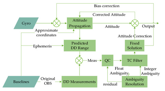
Figure 1.
Flow chart of tightly coupled attitude determination.
3. GNSS Observation Quality Control
The half-cycle slips and multipath errors in the carrier phase will destroy the integer characteristics of the ambiguity, increasing the difficulty of confirming a reliable integer ambiguity candidate. For example, the ratio test cannot be passed. Additionally, the errors of the carrier observation will be absorbed by the non-ambiguity parameters of the fixed solution, reducing the actual accuracy of the fixed solution.
To further improve the ambiguity resolution success rate and the accuracy of the fixed solution in a harsh environment, we design a practical quality-control method, namely MEMS Attitude-aided Quality-Control (MAQC) method, to detect and eliminate outliers in the single-frequency single-epoch mode. The MAQC method benefits from the MEMS precise attitude and can gradually eliminate outliers from large to small by iteration steps, which can reduce the possible misjudgment caused by large outliers and can obtain the ability to detect small outliers.
The procedure for the MAQC method is: (1) quickly eliminate bigger outliers in the data pre-processing step. Specifically, use the baseline length and MEMS attitude to predict DD pseudo-range and carrier phase observations. Then calculate the detector to quickly detect those observations containing large error. Eliminate the observations that exceeding the threshold before the KF measurement update. (2) After the KF measurement is updated, the ratio test and the posteriori residual of DD carrier phase with fixed ambiguity are performed. If the ratio test is failed, the observations with the largest residual are eliminated and then the KF measurement update is performed again. When the ratio test is passed, or the number of carrier measurements of the two baselines has been reduced to 3, the MAQC method ends.
The following details the principle of the MAQC method and Algorithm 1 summarizes the key steps and variables.
- (1)
- Quickly eliminate bigger outliers in the data pre-processing step.
Considering half-cycle slips and multipath errors in the GNSS observations, the observation equation can be expressed as [22,29]
where represents the multipath error (unit: m) and the half-cycle slip value (±1). The other symbols are the same as in Formula (11). The pseudo-range multipath error can reach tens of meters. The non-difference carrier phase multipath error does not exceed a quarter of a wavelength at most. A half-cycle slip causes a half wavelength bias.
Predict the DD station-satellite distance by Formula (12). The differences between and the DD pseudo-range and carrier phase observations are the predicted residuals, expressed as:
When the MEMS attitude accuracy is 2 degrees, the max predicted error of the double-difference station with a 1 m baseline is about 4 cm. At this moment, the accuracy of the DD pseudo-range residuals is determined by (meter-level), which is capable of detecting the DD pseudo-range multipath errors. include DD integer ambiguity, half-cycle slip, phase multipath error, (millimeter level) and (centimeter level). The accuracy of estimated DD ambiguity is mainly determined by , and an error of 4 cm will lead to the error of about 0.2 cycles for GPS L1. If there is a half-cycle slip, the error would be 0.5 cycles or so.
We use the decimal part of the estimated DD ambiguity to detect half-cycle slips and multipath errors. In addition, the DD pseudo-range predicted residuals are used to detect multipath errors. The detectors and can be expressed as:
where and are the outlier judgment thresholds. The attitude covariances output from the central filter are used to evaluate the thresholds in real time. The formulas are expressed as:
where represents the standard deviation of .
It should be pointed out that the thresholds are not constant for different pairs of satellites and baseline lengths. Additionally, the filter covariances of the attitudes may not match well with actual error propagation, especially for a long period time. When the GNSS outage lasts for quite a long time, due to the accumulation of attitude errors, the threshold becomes unreliable. The effective time needs to be set. Once the effective time is exceeded, the detection should stop. The specific threshold is determined by the performance of MEMS.
- (2)
- Ratio test and the posteriori residuals with integer ambiguity fixed.
After the preliminary elimination in pre-processing, the remaining observations and the MEMS predicted state can usually obtain a more reliable fixed solution. If the ratio test fails, the posteriori residuals are used to further eliminate the poor-quality observations that obstruct the ambiguity resolution.
In the float solutions, the biases in the observations will be absorbed by the ambiguity parameters, and the posteriori residuals may not necessarily reflect the real quality of the observations. In the tight coupled mode, MEMS provides high-precision state prediction information, and integer ambiguity candidate is more reliable. The posteriori residual of the observation obtained by fixing the ambiguity can more truly reflect the outliers. By iteratively eliminating the observation with the largest posteriori residual, the outliers that hold back the determination of the ambiguity resolutions can be quickly removed. It is our experience that the number of iterations is usually less than three.
The formula to calculate the ambiguity-fixed residuals is
After the observation with the largest residual is eliminated, the KF measurement update and the ratio test will be performed again. Until the ratio test is passed, or the number of (DD carrier phase) of the two baselines both has been reduced to 3, the iteration ends.
| Algorithm 1. MEMS Attitude aid Quality-Control (MAQC) |
| Task: Eliminate observations that contain relatively large bias: |
| Parameters: , , , , |
| Initialization: n1 = count (), n2 = count () Fast Elimination: 1. calculate by the Formula (12) 2. calculate detector , by the Formula (21) 3. calculate , by the Formula (22) 4. eliminate the observations if or |
| Iterative Elimination: 1. update the ratio, n1 and n2 While (ratio < 3 and (n1 > 3 or n2 > 3)), do: |
| 2. calculate measurement residuals of fixed solution by the Formula (23) |
| 3. eliminate the observation if its residual is the max one |
| 4. update the ratio, n1 and n2 |
| End while |
| Output: relatively high-quality observations |
It should be noted that the ratio test is one of the oldest and most popular ways of validating integer ambiguity solutions [30]. Usually, the integer ambiguity candidate is considered to be reliable when the ratio is bigger than 3, but it does not mean the definitely right. It is useful to add other methods such as baseline length check to ensure more reliable ambiguity resolutions.
4. Results
4.1. Data Collection and Processing Strategy
To test the multi-antenna GNSS/MEMS single-frequency single-epoch tightly coupled attitude determination system and the MAQC method, two vehicle experiments were conducted in urban environments. The first experiment was conducted in a relatively open suburban environment, and was used to test the validity and accuracy of the tightly coupled system. The second experiment, conducted in an urban canyon, aimed to analyze and verify the performance of GNSS/MEMS tightly coupled attitude determination and MAQC methods in harsh environment.
The experimental platform is equipped with 3 GNSS receivers (Septentrio Mosaic-×5, Leuven, Belgium) with a sampling frequency of 1 Hz; A low-cost MEMS IMU (ADIS-16460) and a high-precision tactical grade IMU (SPAN FSAS) are installed. Their gyroscopes’ specifications are shown in Table 1. Three GNSS antennas are used on the roof of the car, forming two baselines of 1.12 m (Baseline 1, BL1, aligned in driving direction) and 0.99 m (Baseline 2, BL2, right-angled to BL1). The equipment setup in is shown in Figure 2. The GNSS base station, set up in the center of the experiment area, uses the Trimble Net R9 receiver and measurement antennas, and the sampling frequency is 1 Hz.

Table 1.
Specifications of the gyroscopes in the AIDS16460 and the SPAN-FSAS.
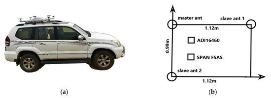
Figure 2.
Equipment setup for vehicle experiments: (a) the experimental vehicle; (b) equipment setup diagram.
Three modes for attitude determination—multi-antenna GNSS attitude determination with direct method (GNSS mode), multi-antenna GNSS/MEMS tightly coupled attitude determination (TC mode), multi-antenna GNSS/MEMS tightly coupled attitude determination with MAQC quality-control (TC-QC mode)—were adopted to demonstrate the performance of different methods for attitude determination in different environments. For all modes above, GPS L1 and BDS B1 GNSS observations were used for data processing. The elevation mask angle of the satellite was 10 degrees. The carrier ambiguity processing strategy was single-epoch mode, and thus the ambiguity information between epochs was not inherited.
The attitude reference is obtained by using the commercial post-processing software Inertial Explorer (IE) to process dual-frequency GNSS/SPAN FSAS integrated navigation data. The post-processing mode is tightly coupled RTK/INS forward and backward filtering and smoothing.
4.2. An Open Environment
In this section, we use the vehicle experiment performed in a GNSS friendly environment to evaluate the effectiveness of the TC mode and the MAQC method. In addition, several GNSS outages were simulated to show the attitude drift of MEMS. Here is a brief introduction of the experiment results: in terms of the ambiguity resolution success rates, the results for the three modes were 97.27 (BL1)/97.07% (BL2), 95.0% (TC), 100.0% (TC-QC); in terms of the accuracy of attitude determination, TC and TC-QC were almost the same, with the accuracy of attitude angle being 0.12, 0.21, and 0.17 degrees for yaw, pitch and roll angle, respectively which is better than the accuracy of GNSS alone; the MAQC method can detect and eliminate observations with bias greater than 0.1 cycle, which explains why the ambiguity resolution success rate of the TC-QC mode rises to 100%. When the GNSS signal suffers a block within 2 min, the attitude drift was limited to within 2 degrees when relying on MEMS gyroscopes.
This experiment was carried out in an industrial park, with a relatively open field. The data duration was 3000 s, and the vehicle’s trajectory is shown in Figure 3a. Figure 3b–d show the number of visible satellites and observation quality during the experiment time. The number GPS+BDS visible satellites for most epochs was more than 20. In a few epochs, the number of satellites dropped sharply, mainly due to the influence of large vehicles, trees and building obstructions, but there were still more than 10 satellites.
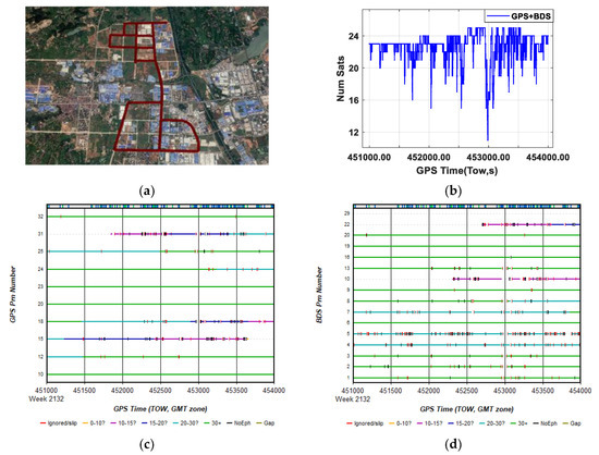
Figure 3.
First experiment in an open environment: (a) trajectory of vehicle; (b) number of visible satellites of the primary baseline; (c) the GPS L1 “Satellite Lock—Cycle Slips” plot from IE; (d) the BDS B1 “Satellite Lock—Cycle Slips” plot from IE.
Firstly, the performance of three attitude determination modes in the favorable environment are evaluated. To make a relatively reliable comparison, the attitude result (SPAN FSAS) obtained from IE is used as a reference. In addition, the installation angle deviations between the GNSS baselines axes and the two IMUs are calculated and compensated. Then the time series of three modes’ attitude errors are shown in Figure 4, and the RMS and STD of the attitude errors are counted (see Table 2). It should be noted that only the ambiguity-fixed solutions of GNSS mode are plotted.
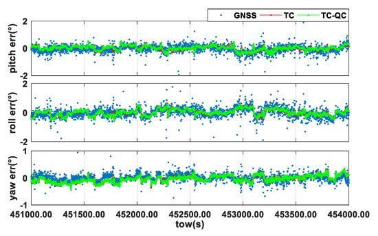
Figure 4.
Time sequence of attitude errors.
Table 2.
Statistics of attitude errors (Unit: degree).
On the whole, both Figure 4 and the statistics given in Table 2 show that the attitude error of the TC mode is smaller than that of the GNSS mode, from 0.13, 0.25, and 0.29 degrees to 0.12, 0.21, and 0.17 degrees. At the same time, it can be seen that regardless of the modes, the accuracy of the yaw angle is the highest, while the accuracy of the pitch and roll angles are poorer. In the GNSS mode, this is because the baseline horizontal components for determining the heading angle have relatively small errors, while the baseline vertical component for determining the pitch angle and roll angle has a relatively large error. In the TC mode, the accuracy of the three attitude angles also has the same characteristics. The essence is that the strength of GNSS measurements in the horizontal direction is greater than that in the vertical direction.
Because the quality of observations was quite high, MAQC did not contribute to a significant increase in attitude accuracy.
To evaluate the ability of the MAQC method to detect outliers, we chose the three satellites C08, C09, and C13 observed in baseline 1 as examples, and the reference satellite was C06. Figure 5a shows the predicted residuals of carrier observations over time. Figure 5b shows the predicted residuals of the double difference phase observations passed through the MAQC method. The red line is the threshold line. It can be seen that the original phase residuals contain some half-cycle slips and multi-path errors. When using the MAQC method to eliminate the observations containing large bias, the phase residuals become stable and smooth.
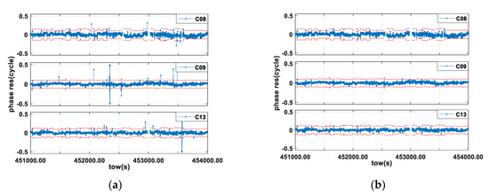
Figure 5.
Residuals of carrier phase in real experiment: (a) prediction residuals of carrier phase; (b) residuals of the retained carrier phase measurements by MAQC method. The rea lines symbolize threshold value. The blue lines symbolize the residuals.
The time period with the best data observation quality (451,000–452,000 s) was selected for the simulation experiment. A small error of +0.2 cycles was added to the L1-frequency carrier phase observation of the C08, C09 and C13 satellites observed by the main antenna every 10 s, and the MAQC method was used to detect and eliminate the observations containing the bias.
Figure 6a shows the residuals of the phase observations with a large number of small errors, and Figure 6b shows the residuals of the phase observations after processing. Most of the observations with small errors are eliminated.
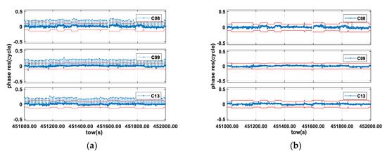
Figure 6.
Residuals of carrier phase in simulated experiment: (a) prediction residuals of carrier phase; (b) residuals of the retained carrier phase measurements by MAQC method. The rea lines symbolize the threshold value. The blue lines symbolize the residuals.
To compare the ambiguity resolution success rates of the three modes, we take the ratio test as the standard: when the ratio is greater than 3, it is assumed that the ambiguities are correctly fixed. Based on this judgement, the ambiguity resolution success rates of the BL1 and BL2, TC mode and TC-QC mode can be counted (see Figure 7).
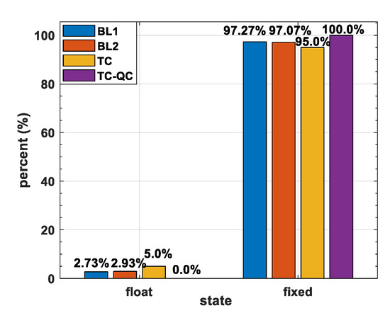
Figure 7.
Success rates of ambiguity resolution.
For the favorable observation environment, both the ambiguity resolution success rates of BL1 and BL2 of are above 97% in the single-frequency single-epoch mode. The ambiguity fixed rate of the TC mode is slightly reduced, to 95%. The reason for this is that the observation outliers of the two baselines all gather in one equation, disturbing more epochs to perform successful ambiguity resolution in TC mode. With the MAQC method eliminating the difficult-to-fix carrier observations effectively, the ambiguity resolution success rate of the TC-QC mode reaches 100%.
When the GNSS experiences an outage, it can only rely on MEMS to maintain the attitude output. During that time, the performance of the MEMS gyroscope determines the accuracy of the attitudes. In the tightly coupled mode, the gyro biases are estimated and compensated. The performance of the MEMS gyroscopes can be significantly improved through the compensation operation, thereby slowing down the accumulation of attitude errors.
The time series of three gyro bias estimated axes are plotted in Figure 8a. It shows that the gyro biases of the three axes are about (300, 90, 1000)°/h. If the gyro bias of the z-axis is not compensated, it is easy to predict that the angle drift of z-axis can reach about 30 degrees in 2 min and lead to a huge attitude error. Assuming that the z-axis gyro bias is well compensated, and the residual bias is about 24°/h, three times the nominal bias stability (8°/h, 1), it can be predicted that a 2 min outage will lead to an accumulated attitude error of 0.8 deg.
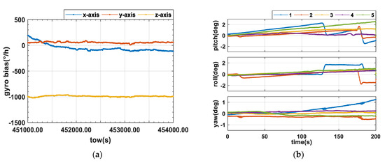
Figure 8.
(a) MEMS gyro bias of each axis; (b) attitude drift of MEMS alone.
To evaluate the independent attitude determination capability of the MEMS gyroscopes more realistically, five sets of 200 s time periods with GNSS completely blocked were simulated using the first experiment data. Figure 8b shows the attitude drift during the five periods. It can be seen that within 2 min, the pitch angle drift is about 2 degrees, and the yaw and roll angle drifts are about 0.5 degrees. This is approximately similar to the prediction above. The improvement of the MEMS performance is significant.
It should be noted that a certain amount of time is required for the TC mode to accurately estimate the gyro bias. Figure 8a shows that the convergences of the MEMS x- and y-axis gyro bias estimation are relatively slower than that for the z-axis. It is because the accuracy of yaw angle is higher than that of pitch and roll, which is beneficial to sensing the gyro bias of the z-axis, which is more related to the yaw angle. Figure 8b shows that the attitude error of the first simulation segment is relatively large, because this segment is at the initial stage, and the estimation of the gyro bias is not accurate enough.
The performance of the MEMS gyroscopes alone also determines the effectiveness of the MAQC method. It relies on accurate attitudes predicted by MEMS to ensure that the MAQC method possesses a reliable capability to detect outliers within a certain period of GNSS outage. For a baseline with the length of 1 m, a 2-degree attitude error will result in a prediction error of about 4 cm, which is much smaller than the GPS L1 half-cycle wavelength. This shows that the MAQC method has the ability to detect half-cycle slips within 2 min of GNSS outage.
4.3. A Challenging Urban Environment
In this section, we use an urban canyon vehicle experiment to compare the attitude accuracy and ambiguity resolution success rates of the three attitude determination modes in harsh environments, and verify the detection capability of MAQC. The experimental results show that the ambiguity resolution success rates of the GNSS mode are less than 70% in the single-frequency single-epoch mode, while in the TC mode, they increase to above 90%, with the attitude accuracy significantly improved. The ambiguity resolution success rate of the TC-QC mode reaches nearly 98%, and the attitude accuracy is further improved, which verifies the benefit of the MAQC method in the urban environment.
This experiment was carried out in downtown Wuhan, with a relatively harsh environment. The data duration was 1000 s, and the vehicle trajectory is shown in Figure 9a. Figure 9b–d show the number of visible satellites and observation quality during the experiment time. The number of GPS+BDS visible satellites drops suddenly or even to zero in a large number of epochs with heave blocks.
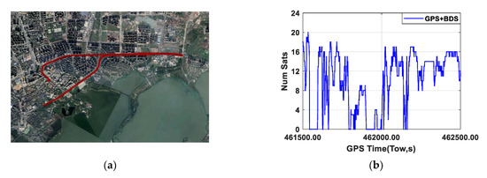
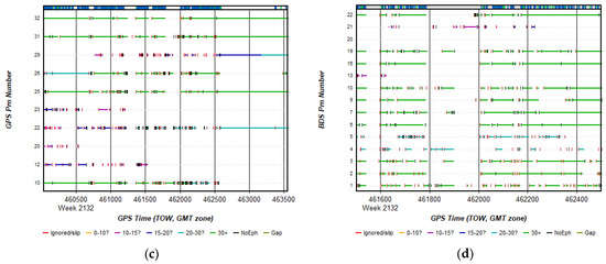
Figure 9.
Second experiment in a challenged urban environment: (a) trajectory of vehicle; (b) the number of visible satellites of primary baseline; (c) the GPS L1 “Satellite Lock—Cycle Slips” plot from IE; (d) the BDS B1 “Satellite Lock—Cycle Slips” plot from IE.
Using the reference attitude (SPAN FSAS) obtained from IE and the installation angle deviations compensated, the attitude errors of the three modes are obtained. Figure 10 shows their comparison. Table 3 lists their RMS and STD.
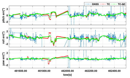
Figure 10.
Time sequence of attitude errors.
Table 3.
Statistics of attitude errors (Unit: degree).
As shown in Figure 10, the availability of GNSS mode attitude determination is very poor, while the TC and TC-QC mode have continuous and stable performance. In Table 3, the accuracy of attitude determination in GNSS mode is 3.167, 3.344, and 6.773 degrees for yaw, pitch and roll, respectively, which is far worse than that (0.13, 0.25, and 0.29 degrees) in the friendly environment. This is because many epochs fixed the ambiguity wrongly, leading to false attitude results far from the true value. This proves that attitude determination based on GNSS alone is unreliable in harsh environments.
In TC mode, the errors of the heading, pitch, and roll angles are 0.298, 0.462, and 0.408 degrees, respectively. Compared with GNSS mode, it is reduced by 90% or more, which is a significant improvement. The attitude accuracy of the TC-QC mode is further improved compared to that of the TC mode. Especially in the heading angle, the RMS reduced from 0.321 degrees to 0.196 degrees. Figure 10 shows the feature that the mainly improvement of TC-QC mode is when the GNSS observation environment is very bad or unavailable.
The prediction residual sequence of the carrier observation value before and after using the MAQC method was plotted. Due to the large number of satellites and each star having its own threshold line, to keep the map concise, the satellite threshold lines are no longer drawn.
The residual error of the carrier observation value screened by the MAQC method is shown in Figure 11b. The residuals of the retained measurement values are all small, which proves the reliability of the MAQC method.
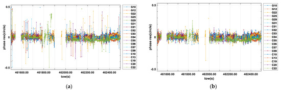
Figure 11.
Residuals of the carrier phase: (a) residuals of the carrier phase measurements; (b) residuals of the retained carrier phase measurements by MAQC method.
To compare the ambiguity resolution success rates in the urban environment, only GNSS available epochs are counted. The criterion for valid epoch is that the number of double-difference carrier phase observations of the main baseline is not less than 3, and 783 epochs met this requirement.
The epoch counts for different number of available DD phase observations are shown in Figure 12a. The success rates of the ambiguity resolution in the urban environment are presented in Figure 12b. In addition, the global success rates for all epochs in four attitude determination modes are shown in Figure 12c. Figure 12b,c show that the TC-QC mode obtains the highest ambiguity resolution success rates on the whole. When the number of carrier phase double difference observations is greater than or equal to 6, it is close to 100%. TC mode behaves well, with most rates being over 90%. The success rates of baseline solutions with GNSS alone are very low, which are significantly lower than those in Experiment 1. When the number of observations is less than 10, the success rates of the two baselines are below 50%, and when the number of observations exceeds 12, the success rates can reach 80%. The reason for this is that the multipath effect is extremely heavy in the urban environment, making the float solution unreliable. When using the TC mode, benefiting from the high-precision MEMS prediction state, better float solutions can be achieved.
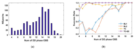
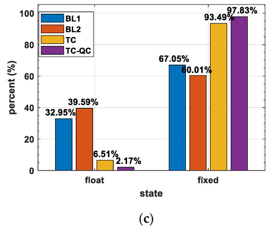
Figure 12.
Success rates of ambiguity resolution: (a) epoch counts for different numbers of available DD phase observations; (b) success rates for different number of available DD phase observations; (c) global success rates for all epochs in 4 attitude determination modes.
5. Discussion
MEMS plays a role in predicting the system state and smoothing the attitude output. Meanwhile, the quality of GNSS observations dominates the ultimate accuracy of TC attitude determination. In the GNSS-friendly experiment, the RMS of the TC GNSS/MEMS attitudes were 0.12, 0.21, and 0.17 degrees, slightly smaller than the RMS (0.13, 0.25, 0.29) degrees of the GNSS fixed solutions. Meanwhile, the waves and peaks in the time series of attitude error in Figure 4 show a high consistency between the TC mode and GNSS mode. The above results imply the absolute accuracy is dominated by GNSS.
In the TC mode, the MEMS-predicted system state can directly assist the ambiguity resolution, improving the success rate and the accuracy of the attitude determination. The urban environment experiment shows that the success rate of TC ambiguity resolution is significantly increased to above 90%, and the accuracy of yaw, pitch and roll is increased from 3.167, 3.344, and 6.773 degrees to 0.298, 0.462, and 0.408 degrees, respectively. Insufficient GNSS observations and degradation of observation quality hinder the ambiguity resolution success rate and degrade the accuracy of attitude determination. With the MAQC, the success rate is increased to 97.8%, and the accuracy is further improved. The experiment adopts the GPS+BDS systems, and the valid epoch in the urban environment is only about 78%. If the Multi-GNSS satellites can be observed at the same time, it is expected to increase effective observations and further improve the availability and accuracy of coupled attitude determination.
Tight combination has the advantage that even only two satellite observations can play a role in KF measurement update. The influence of this feature on attitude determination can be further explored in the future. Additionally, the accelerometer in the MEMS IMU can be used to estimate the pitch and roll angle when stationary [12], which has not yet been incorporated into our model. Adding this measurement to the determination of the attitude could further improve the accuracy of the pitch and roll angle. The use of the accelerometer to measure attitude needs to eliminate the interference of line of sight acceleration, which can be reduced or eliminated by means of sliding window averaging and GNSS position assistance during the maneuver [6,15].
6. Conclusions
In this paper, a new tightly coupled multi-antenna GNSS/MEMS attitude determination model was constructed, using a single filter to achieve the optimal estimation of ambiguities, attitude drift and gyro biases. The filter state includes both GNSS and MEMS parameters, leading to a tighter combination than the existing models we found for multi-antenna GNSS/MEMS attitude determination. The fixed solutions of the tightly coupled mode, compared with that comes from GNSS alone, had a reduction of attitude errors from (0.251, 0.290, 0.129) degrees to (0.12, 0.21, 0.17) degrees in favorable environments for heading, pitch, and roll angles, respectively, and from (3.344, 6.773, 3.167) degrees to (0.32, 0.54, 0.46) degrees in challenging environments. As for the ambiguity resolution success rate, it was greatly increased as well—from 67% to 93%.
With the proposed quality-control method, namely MAQC, observation outliers that drag down the process of fixed ambiguity solution can be eliminated effectively, thus guaranteeing both the fixed rate of ambiguity and the higher accuracy of estimations. With the MAQC method in the single-frequency single-epoch mode, the ambiguity resolution success rate reached 100% in a favorable environment, and reached about 98% in challenging environments. Additionally, compared with that of the tightly coupled mode without MAQC, the accuracy of heading, pitch, and roll angles was improved by 38.94%, 7.43%, 4.98%, respectively in the challenging environment, showing a further enhancement of the attitude accuracy when using the MAQC method.
Author Contributions
Conceptualization, M.G.; Data curation, G.L.; Formal analysis, G.X. and D.L.; Methodology, M.G.; Project administration, G.L.; Resources, G.L.; Software, M.G., S.W. and W.Z.; Supervision, G.L.; Validation, W.Z.; Visualization, S.W. and G.X.; Writing—original draft, M.G.; Writing—review & editing, S.W., G.X., W.Z. and D.L. All authors have read and agreed to the published version of the manuscript.
Funding
This work was jointly supported by the National Key Research Program of China Collaborative Precision Positioning Project (No. 2016YFB0501900) and the National Natural Science Foundation of China (Grant No. 41774017).
Acknowledgments
The authors would like to thank Shilong Cao and Chengfeng Zhang for their help in setting up the multi-sensor platform used in the vehicle experiments. Meanwhile, the authors are grateful to Aizhi Guo for his valuable advice in writing.
Conflicts of Interest
The authors declare no conflict of interest.
References
- Teunissen, P.J.G. Integer least-squares theory for the GNSS compass. J. Geod. 2010, 84, 433–447. [Google Scholar] [CrossRef]
- Chang, X.; Yang, X.; Zhou, T. MLAMBDA: A modified LAMBDA method for integer least-squares estimation. J. Geod. 2005, 79, 552–565. [Google Scholar] [CrossRef]
- Teunissen, P.J.G. The least-squares ambiguity decorrelation adjustment: A method for fast GPS integer ambiguity estimation. J. Geod. 1995, 70, 65–82. [Google Scholar] [CrossRef]
- Zhang, P.; Zhao, Y.; Lin, H.; Zou, J.; Wang, X.; Yang, F. A Novel GNSS Attitude Determination Method Based on Primary Baseline Switching for A Multi-Antenna Platform. Remote Sens. 2020, 15, 747. [Google Scholar] [CrossRef]
- Emel’yantsev, G.; Stepanov, O.; Stepanov, A.; Blazhnov, B.; Dranitsyna, E.; Evstifeev, M.; Eliseev, D.; Volynskiy, D. Integrated GNSS/IMU-Gyrocompass with Rotating IMU. Development and Test Results. Remote Sens. 2020, 12, 3736. [Google Scholar] [CrossRef]
- Zhu, F.; Hu, Z.; Liu, W.; Zhang, X. Dual-Antenna GNSS Integrated With MEMS for Reliable and Continuous Attitude Determination in Challenged Environments. IEEE Sens. J. 2019, 19, 3449–3461. [Google Scholar] [CrossRef]
- Ma, L.; Lu, L.; Zhu, F.; Liu, W.; Lou, Y. Baseline length constraint approaches for enhancing GNSS ambiguity resolution: Comparative study. GPS Solut. 2021, 25. [Google Scholar] [CrossRef]
- Cai, T.; Xu, Q.; Gao, S.; Zhou, D. A Short-baseline Dual-antenna BDS/MIMU Integrated Navigation System. In Proceedings of the 3rd International Conference on Power, Energy and Mechanical Engineering, Prague, Czech Republic, 16–19 February 2019; Volume 95. [Google Scholar]
- Patrick, H.; Günther, C.; Inst, N. Attitude determination with low-cost GPS/INS. In Proceedings of the 26th International Technical Meeting of the Satellite Division of the Institute of Navigation, Nashville, TN, USA, 16–20 September 2013; Inst Navigation: Washington, DC, USA, 2013; pp. 2015–2023. [Google Scholar]
- Eling, C.; Zeimetz, P.; Kuhlmann, H. Development of an instantaneous GNSS/MEMS attitude determination system. GPS Solut. 2013, 17, 129–138. [Google Scholar] [CrossRef]
- Li, W.; Fan, P.; Cui, X.; Zhao, S.; Ma, T.; Lu, M. A Low-Cost INS-Integratable GNSS Ultra-Short Baseline Attitude Determination System. Sensors 2018, 18, 2114. [Google Scholar] [CrossRef] [PubMed]
- Eling, C.; Klingbeil, L.; Kuhlmann, H. Real-time single-frequency GPS/MEMS-IMU attitude determination of lightweight UAVs. Sensors 2015, 15, 26212–26235. [Google Scholar] [CrossRef]
- Hirokawa, R.; Ebinuma, T. A low-cost tightly coupled GPS/INS for small UAVs augmented with multiple GPS antennas. Navigation 2009, 56, 35–44. [Google Scholar] [CrossRef]
- Hwang, D.H.; Oh, S.H.; Lee, S.J.; Park, C.; Rizos, C. Design of a low-cost attitude determination GPS/INS integrated navigation system. GPS Solut. 2005, 9, 294–311. [Google Scholar] [CrossRef]
- Wu, Z.; Yao, M.; Ma, H.; Jia, W. Low-cost attitude estimation with MIMU and two-antenna GPS for Satcom-on-the-move. GPS Solut. 2013, 17, 75–87. [Google Scholar] [CrossRef]
- Cai, X.; Hsu, H.; Chai, H.; Ding, L.; Wang, Y. Multi-antenna GNSS and INS Integrated Position and Attitude Determination without Base Station for Land Vehicles. J. Navig. 2018, 72, 342–358. [Google Scholar] [CrossRef]
- Daneshmand, S.; Lachapelle, G. Integration of GNSS and INS with a phased array antenna. GPS Solut. 2017, 22. [Google Scholar] [CrossRef]
- Emel’yantsev, G.; Dranitsyna, E.; Stepanov, A.; Blazhnov, B.; Vinokurov, I.; Kostin, P.; Petrov, P.; Radchenko, D. Tightly-Coupled GNSS-Aided Inertial System with Modulation Rotation of Two-Antenna Measurement Unit; 2017 DGON Inertial Sensors and Systems (ISS): Karlsruhe, Germany, 2017; pp. 1–18. [Google Scholar] [CrossRef]
- Wang, Y.; Zhao, X.; Pang, C.; Wang, X.; Wu, S.; Zhang, C. Improved pitch-constrained ambiguity function method for integer ambiguity resolution in BDS/MIMU-integrated attitude determination. J. Geod. 2018, 93, 561–572. [Google Scholar] [CrossRef]
- Cong, L.; Li, E.; Qin, H.; Ling, K.V.; Xue, R. A performance improvement method for low-cost land vehicle GPS/MEMS-INS attitude determination. Sensors 2015, 15, 5722–5746. [Google Scholar] [CrossRef]
- Oh, S.H.; Hwang, D.-H.; Park, C.; Lee, S.J. Attitude Determination GPS/INS Integration System Design Using Triple Difference Technique. J. Electr. Eng. Technol. 2012, 7, 615–625. [Google Scholar] [CrossRef][Green Version]
- Henkel, P.; Oku, N. Cycle Slip Detection and Correction for Heading Determination with Low-Cost GPS/INS Receivers. In Proceedings of the VIII Hotine-Marussi Symposium on Mathematical Geodesy, Rome, Italy, 17–21 June 2013; Springer: Cham, Switzerland, 2016; pp. 291–299. [Google Scholar]
- Wang, Z.; Chen, W.; Dong, D.; Wang, M.; Cai, M.; Yu, C.; Zheng, Z.; Liu, M. Multipath mitigation based on trend surface analysis applied to dual-antenna receiver with common clock. GPS Solut. 2019, 23. [Google Scholar] [CrossRef]
- Yang, Y.; Mao, X.; Tian, W. A novel method for low-cost MIMU aiding GNSS attitude determination. Meas. Sci. Technol. 2016, 27, 075003. [Google Scholar] [CrossRef]
- Groves, P.D. Principles of GNSS, Inertial, and Multisensor Integrated Navigation Systems, 2nd ed.; Artech House: London, UK, 2013. [Google Scholar]
- Godha, S.; Cannon, M.E. GPS/MEMS INS integrated system for navigation in urban areas. GPS Solut. 2007, 11, 193–203. [Google Scholar] [CrossRef]
- Genyou, L.; Jikun, O. Determining Attitude with Single Epoch GPS Algorithm and Its Precision Analysis. Geomat. Inf. Sci. Wuhan Univ. 2003, 28, 732–735. [Google Scholar]
- Teunissen, P.J.G. The affine constrained GNSS attitude model and its multivariate integer least-squares solution. J. Geod. 2011, 86, 547–563. [Google Scholar] [CrossRef]
- Dong, D.; Wang, M.; Chen, W.; Zeng, Z.; Song, L.; Zhang, Q.; Cai, M.; Cheng, Y.; Lv, J. Mitigation of multipath effect in GNSS short baseline positioning by the multipath hemispherical map. J. Geod. 2015, 90. [Google Scholar] [CrossRef]
- Teunissen, P.J.G.; Verhagen, S. On the foundation of the popular ratio test for GNSS ambiguity resolution. In Proceedings of the ION GNSS, Long Beach, CA, USA, 21–24 September 2004; pp. 2529–2540. [Google Scholar]


Publisher’s Note: MDPI stays neutral with regard to jurisdictional claims in published maps and institutional affiliations. |
© 2021 by the authors. Licensee MDPI, Basel, Switzerland. This article is an open access article distributed under the terms and conditions of the Creative Commons Attribution (CC BY) license (https://creativecommons.org/licenses/by/4.0/).