An Automatic Method to Detect Lake Ice Phenology Using MODIS Daily Temperature Imagery

Abstract

Lake ice phenology is a climate-sensitive indicator. However, ground-based monitoring suffers from the limitations of human vision and the difficulty of its implementation in harsh environments. Remote sensing provides great potential to detect lake ice phenology. In this study, a new automated method was developed to extract lake ice phenology parameters by capturing the temporal pattern of the transitional water/ice phase using a parameterized time function. The method is based on Moderate-Resolution Imaging Spectroradiometer (MODIS) daily temperature products, which have unique potential for monitoring lake ice cover as a result of providing four observations per day at 1 km spatial resolution from 2002 to 2016. Three seasonally ice-covered lakes with different characteristics in different climate regions were selected to test the method during the period of 2002–2016. The temporal pattern of water/ice transition phase was determined on the basis of unfrozen water cover fraction extracted from the MODIS daily temperature data, and was compared with the MODIS snow and reflectance products and Landsat images. A good agreement with an R² of above 0.8 was found when compared with the MODIS snow product. The annual variation of extracted ice phenology dates showed good consistency with the MODIS reflectance and AMSR-E/2 products. The approach was then applied to nine seasonally ice-covered lakes in northern China from 2002 to 2016. The strongest tendency towards a later freeze-up start date was revealed in Lake Qinghai (6.31 days/10 yr) among the lakes in Tibetan plateau, and the break-up start and end dates rapidly shifted towards earlier dates in Lake Hulun (−3.73 days/10 yr; −5.02 days/10 yr). The method is suitable for estimating and monitoring ice phenology on different types of lakes over large scales and has a strong potential to provide valuable information on the responses of ice processes to climate change.

1. Introduction

Lake ice phenology, which encompasses freeze-up and break-up periods/dates and ice cover duration, is important for the biological, chemical and physical processes of lakes, especially in cold regions [1,2]. Long-term records of ice phenology serve as sensitive indicators of climate variability [3]. Increases in the interannual variability in lake ice phenology have been found in recent studies [4,5,6]. Ice freeze-up occurs later and ice break-up earlier, with the result of ice cover being lost at an accelerating rate in the Northern Hemisphere [2,5,6]. These trends in ice phenology are closely related to increasing air temperatures [7,8,9] and to the integrated effects of changing wind speeds, snow cover, and solar radiation [10].

Despite their robustness, ground-based lake ice observations have experienced a global decrease since the 1980s [11]. In turn, satellite remote sensing, as an alternative tool, has played a growing role in lake ice monitoring [12]. The brightness temperatures obtained from microwave satellite sensors, such as the Advanced Microwave Scanning Radiometer for the Earth Observing System (AMSR-E) [13,14], Special Sensor Microwave Imager (SSM/I), and Scanning Multichannel Microwave Radiometer (SMMR) [15,16,17], have demonstrated good performance in detecting ice phenology. While being insensitive to atmosphere constraints, microwave observations are relatively suitable for large lakes due to their coarse spatial resolution.

Visible spectrum sensors have also been widely used for monitoring lake ice dynamics, e.g., the Advanced Very-High-Resolution Radiometer (AVHRR, 1.1 km spatial resolution), the Moderate-Resolution Imaging Spectroradiometer (MODIS), with different spatial resolutions (250 m, 500 m, 1 km), the Visible Infrared Imaging Radiometer Suite (VIIRS), and Sentinel-1 and Sentinel-2 with a higher resolution. Several MODIS products have been used to retrieve lake ice phenology, such as MODIS daily reflectance data [18,19,20,21] and MODIS daily snow products [10,22,23,24]. However, the data from optical sensors are strongly limited by cloud obstruction, especially in regions with strong convection in the lower atmosphere, like the Tibetan plateau [25].

Currently, various methods have been developed to fill data gaps due to cloud coverage, such as multi-sensor data or temporal–spatial combinations [26,27,28,29,30]. Approaches using temporal–spatial combinations have been found to effectively improve data availability by approximately 10%–20% [31,32,33]. Among those methods, the daily temporal combination method is especially beneficial for MODIS daily temperature products, which have a unique advantage over other products by providing four observations from Terra and Aqua with a time step of 4 to 7 hours, thereby increasing the amount of available data. Thus, the daily temporal combination of temperature products from MODIS Terra and Aqua data can reduce cloud contamination at a minimal loss of temporal resolution, which is an appropriate technique to monitor lake ice phenology.

Most previous studies on lake ice phenology have used thresholds for binary classification to extract phenology dates from remote sensing data, such as the threshold obtained from near-infrared reflectance [34], or combined near-infrared and surface temperature values [35,36]. An alternative approach is to use a spatially resolved threshold distribution, e.g., 5% and 95% of a lake area [22,23], to de-noise the time series and to define freeze-up/break-up dates with greater certainty. While fixed threshold methods may be limited to different climatic regimes, dynamic threshold approaches, as listed above, are better suited across different climatic regimes and remote sensing data sources.

Alternatively, characterizing the temporal pattern of water/ice transition process is a potential method to extract lake ice phenology. In this study, we proposed a new automated extraction approach using MODIS daily temperature products based on the time-dependent parameterization of the freezing/thawing process. The approach builds upon the studies on vegetation phenology extraction by a time-dependent curve-fitting model using remote sensing data [37,38,39]. The temporal pattern of water/ice phase transition is similar to the pattern of vegetation growth, but quite clearly recognized and stable for the application of time-dependent curve-fitting model compared with the application for the temporal pattern of vegetation phenology [40,41]. The extraction approach was developed using data from three seasonally ice-covered lakes (Lake Qinghai, Lake Ngoring, and Lake Hulun) that differ in morphometry, salinity, elevation, and climate, and applied afterwards to six Chinese lakes in different climate zones. The spatiotemporal changes observed in the ice phenology were analyzed, and their relationships to climatic and lake-specific factors were discussed.

2. Study Area and Data

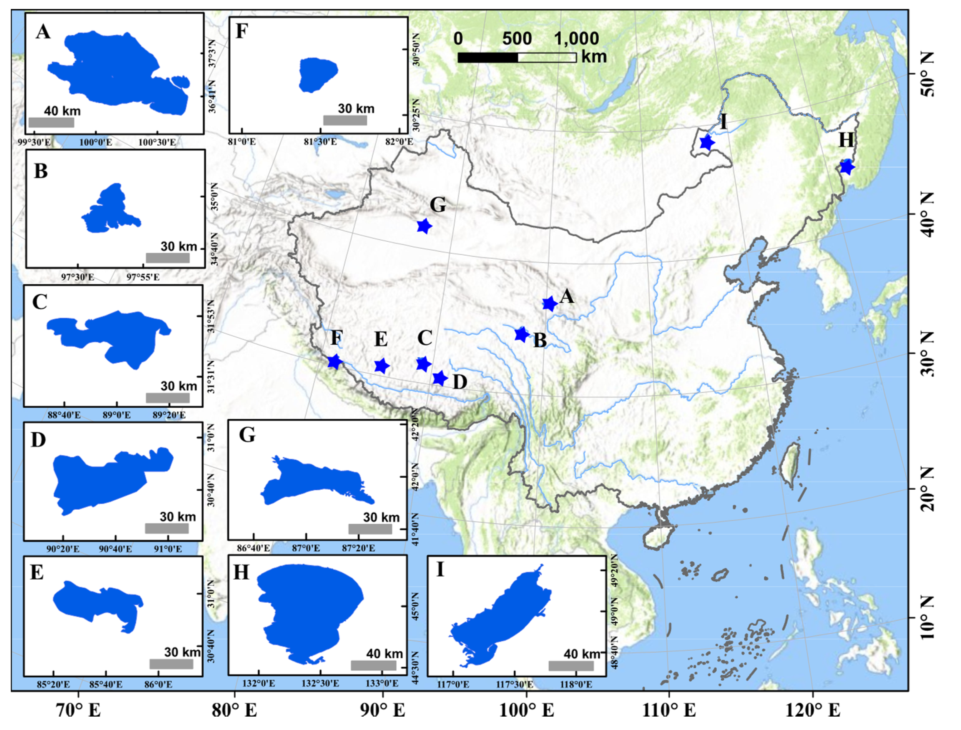
2.1. Study Area

Nine large seasonally ice-covered lakes with different characteristics, latitudes, altitudes, areas, salinities, and climatic conditions distributed across northern China were chosen to develop, evaluate, and test the proposed approach (Figure 1 and

Table 1. The areas, depths, locations, altitude, and salinity for the considered lakes [44].

Lake Name	Lake Area (km2)	Mean Depth (m)	Max Depth (m)	Longitude (°)	Latitude (°)	Altitude (m)	Salinity (g/L)
Lake Qinghai	4340	18	27	100.20	36.88	3260	9.16
Lake Ngoring	611	17	31	97.70	34.90	4272	0.31
Lake Silingco	2390	17	40	88.99	31.79	4539	6.93
Lake Namco	2000	43	70	90.60	30.74	4718	1.78
Lake Zharinamco	1023	4	71	85.63	30.92	4613	13.90
Lake Mapang	412	46	73	81.47	30.68	4585	0.46
Lake Bosten	1646	9	17	87.04	41.97	1045	1.87
Lake Xinkai	4010	5	11	132.42	45.00	68	0.28
Lake Hulun	2044	5	8	117.44	48.97	540	2.40

). Three of the lakes, Lake Qinghai, Lake Ngoring, and Lake Hulun, were selected as target lakes to develop and test the ice phenology extraction algorithm. Lake Qinghai is a large brackish dimictic lake located on the northeastern Tibetan Plateau. It is the largest inland lake in China and is subject to a semiarid continental climate characterized by warm summers, cold winters, and more precipitation in summer than in other seasons [19]. Lake Ngoring is the highest (~4200 m asl) freshwater lake in China and is located in the source region of the Yellow River, surrounded by hills covered with alpine meadows. The south and east shorelines freeze and melt first [42]. Lake Hulun is a shallow monomictic lake located in the eastern part of the Mongolian Plateau in the northern part of China and is affected by semiarid continental and monsoon climates. The lake freezes from the complex shoreline area of the lake, and melting starts from the northwest coast and gradually toward the east coast [43].

2.2. MODIS Data

2.2.1. MODIS Daily Temperature Data

The MODIS sensor mounted on the Terra and Aqua satellites has a total of 36 bands that cover the spectral range from 0.405–14.385 µm. The Terra satellite was launched on 24 February 2000, and the Aqua satellite was launched on 4 June 2002. Daily land surface temperature products from MODIS (MOD11A1, MYD11A1, version 6) were used in the study, with a spatial resolution of 1 km and daily temporal coverage from 2002 to 2016, available on NASA’s Earth Observation System Data and Information System website (https://modis.gsfc.nasa.gov/data/dataprod/mod11.php, accessed on 15 October 2020). The products use the split-window algorithm to retrieve surface temperatures from band 31 and band 32 [45]. The “land” surface temperature products include both land and inland water [46]. The daily temperature data are available four times per day: at approximately 10:30 and 22:30 from Terra and at approximately 1:30 and 13:30 from Aqua (local time).

2.2.2. Other MODIS Data and Landsat Data

The MODIS daily snow product (MOD10A1, version 6) with a spatial resolution of 500 m and daily temporal resolution from 2002 to 2016 was used to compare the temporal pattern of the lake ice cover derived from the MODIS daily temperature product. The MODIS daily snow cover product is available from the U.S. National Snow and Ice Data Center (https://nsidc.org/data/dataprod/mod10.php, accessed on 15 January 2021), and is derived from the SNOWMAP algorithm, which uses the normalized difference snow index (NDSI) and decision strategies to identify snow cover [30,47]. The pixel is labeled as snow when NDSI ≥ 0.4, as recommended by Riggs, G. A. et al. [48]. The land is classified into 6 types: snow, inland water, land, cloud, missing data, and other (unclassified). The assessment showed that MODIS snow cover products have an overall accuracy of ~93% under clear-sky conditions [47]. In this study, we used the snow cover data from Terra only, since the cloud/snow discrimination has errors in Aqua cloud-mask algorithm [30,48]. Additionally, the snow cover data from Aqua in version 6 used band 6 to replace band 7 in the NDSI calculation which is different from the previous version. More details about the MODIS snow products can be found in [30,47,48].

The cloud-free images from the MODIS Daily Reflectance product and Landsat images from 2002 to 2016 were also selected to evaluate the lake water/ice cover information from MODIS temperature products. The MODIS Daily Reflectance product (MOD09GQ, version 6), has a spatial resolution of 500 m and daily temporal resolution, and is available at (https://modis.gsfc.nasa.gov/data/dataprod/mod09.php, accessed on 15 January 2021). The Landsat 5, 7, and 8 images have a high spatial resolution of 30 m and a temporal resolution of 16 days, and are available from the standard United States Geological Survey Landsat Surface Reflectance products. Due to the 16-day temporal resolution and the influence of cloud cover, the availability of Landsat images is limited, and cloud-free images were preferentially selected. In our study, 4 images from Landsat under clear sky condition were chosen in each lake during freeze-up and break-up periods, respectively.

The air temperature from 2002 to 2016 was adopted from the China Meteorological Administration (CMA) dataset which has been checked by thorough quality control [49].

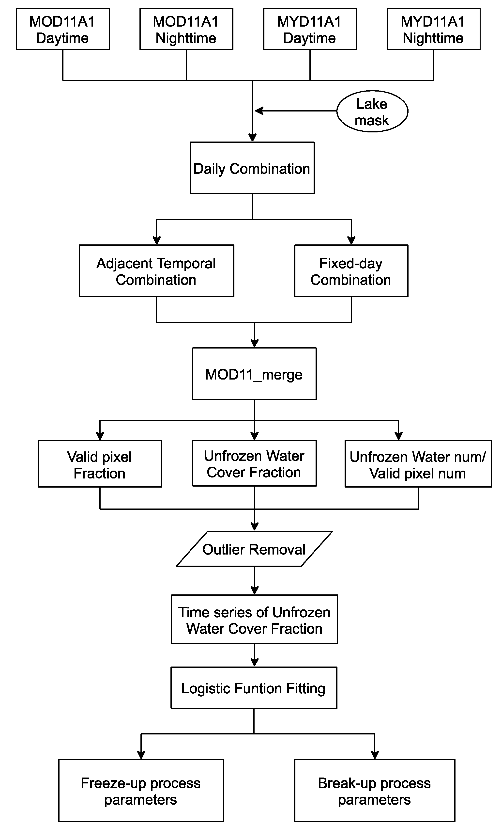
3. Lake Ice Phenology Detection Method

The automated detection of lake ice phenology from MODIS daily temperature data was performed in three main steps (Figure 2): (i) the MODIS data from Terra and Aqua were combined to increase data availability, (ii) the unfrozen water cover fraction was extracted to characterize the spatial-temporal change pattern of water/ice transition, and (iii) a curve-fitting model was applied to capture the ice phenology characteristics in transitional periods. The individual steps of the method are presented in the following sections.

3.1. Terra and Aqua Combination

The lake-extent mask and quality control were applied prior to the Terra and Aqua data combination. The lake mask excluded lake boundaries using a buffer zone (3 × 3-pixel matrix [50,51]) to eliminate the lake-land mixed-pixel effect. Quality control was applied to identify “valid pixels” based on the quality flags from the MOD11A1 and MYDA1 quality control layers. When the pixel quality flags were “good quality”, “average land surface temperature error ≤ 0.01”, “average emissivity error ≤ 0.01”, or “average emissivity error ≤ 0.02”, the corresponding pixels were identified as “valid pixels”. When the pixel quality flags were “cloud effects” or others, the corresponding pixels were identified as “invalid pixels”.

The Terra and Aqua data combination (also referred to as the MODIS Daily combination) referred to merge MOD11A1 and MYD11A1 data acquired on the same day on a pixel-by-pixel basis. Based on the quality flags, the valid pixels were always given priority over invalid pixels. The output temperature images named as MOD11_Merge and the combination was executed by the following step for a single day:

(a) If the same pixel marked as a “valid pixel” was found in more than two images in a given day, the value of the corresponding pixel in MOD11_Merge was calculated by the average temperature from the “valid pixels” and also flagged as “valid”;

(b) If the same pixel marked as a “valid pixel” was found in only one image in a given day, the corresponding pixel in MOD11_Merge was taken from the “valid pixel” and also flagged as “valid”;

(c) If the same pixel marked as a “valid pixel” was not found in any images in a given day, the corresponding pixel was marked as “invalid”.

3.2. Extraction of the Unfrozen Water Cover Fraction

The temporal pattern of water/ice transition phase was determined by unfrozen water cover fraction extracted from MOD11_Merge images during the period 2002–2016. The water/ice status in MOD11_Merge image was classified by a temperature threshold initially on a pixel-by-pixel basis. The temperature thresholds were $\pm 0.5$ °C, here, and their sensitivity analysis was performed as discussed in Section 5.1. The unfrozen water cover fraction was calculated by the number of pixels classified as “water”, accounting for the lake area by the following steps:

(a) If the temperature of the pixel was above 0.5 °C, we regarded the pixel as water and classified it as “Pixel_water”;

(b) If the temperature of the pixel was below −0.5 °C, we regarded the pixel as ice and classified it as “Pixel_ice”;

(c) If the temperature of the pixel was between −0.5 °C and 0.5 °C, we regarded the pixel as starting to freeze (melt) and classified it as “Pixel_{ice-water-mixed}”;

(d) The unfrozen water cover fraction was calculated by Equation (1).

$$\mathrm{Unfrozen}\mathrm{water}\mathrm{cover}\mathrm{fraction}=\frac{{\mathrm{total}\mathrm{number}\mathrm{of}\mathrm{Pixel}}_{water}}{{\mathrm{total}\mathrm{number}\mathrm{of}\mathrm{Pixel}}_{valid}}$$

(1)

Afterwards, the adjacent temporal filter was used on the same pixel in the previous and subsequent days without reducing spatial and temporal resolution to deduce the continuous stable ice-covered or ice-free pixel from cloud-covered pixels. As the adjacent temporal filter was mainly used for stable-status pixel deduction in our study, two temporal windows of $\pm$5 days and $\pm$7 days were chosen, respectively.

Outliers in the unfrozen water cover fraction were mainly caused by the high percentage of cloud cover, as shown in Figure 3. The outliers were eliminated by the following steps. First, the unfrozen water cover fraction was set to 1 for dates before the mean air temperatures in autumn dropped below 0 °C. The mean air temperature values were preliminarily smoothed by a 31-day running average to remove synoptic variability [52]. Second, the unfrozen water cover fraction was removed if the percentage of “invalid” pixels in an image was larger than 80%. After outlier removal, the temporal pattern of the unfrozen water cover fraction (increase or decrease) was applied to describe the water/ice transition process and then extract lake ice phenology.

3.3. Curve Fitting for Lake Ice Phenology Detection

We proposed a time-dependent logistic function to describe the temporal pattern of the unfrozen water cover fraction spanning one hydrological year. The transition between open water and ice-covered states was parameterized by the sigmoidal growth curve, characterized by an initial slow growth, but accelerating thereafter and decreasing in the final phase before approaching the upper asymptote [53]. The growth or decay of the partial ice cover was reflected by variation of the unfrozen water fraction between the limiting values of 1 and 0, where 1 corresponds to open water. The logistic function model has been found to represent the sigmoid growth profile well [37,54] and have frequently been used to fit phenology time series [38,40,41,55]. The logistic function model used here was modified from [37] and is illustrated in Figure 4. The model equation is as follows:

$$y=\frac{a}{1+e^{-k\left(x-x_t\right)}}$$

(2)

where $y$ is the unfrozen water cover fraction at time $x$; $a$ is the maximum value of the unfrozen water cover fraction, which is equal to 1 in our study; $k$ is the rate of curvature at the inflection point, referred as $k_f$ in the freeze-up process and $k_b$ in the break-up process; $x$ is the days of the hydrological year, $x_t$ is the time at a given inflection point, referred to as $x_f$ in the freeze-up process and $x_b$ in the break-up process; and $k$ and $x_t$ are the fitting parameters and represent the curvature and position of function, respectively. The logistic function was similar to the cumulative normal distribution and has two key fitting parameters ($k$ and $x_t$) representing the curvature and position of the function on the time axis, respectively.

The logistic function was applied by fitting $x_t$ and $k$ separately to the freeze-up and break-up periods in each hydrologic year. With $k$ and $x_t$ known, the specific ice phenology characteristics, freeze-up start and end dates (FUS and FUE), break-up start and end dates (BUS and BUE), frozen ice cover duration (days between freeze-up start date and break-up end date, FIC), and complete ice cover duration (days between freeze-up end date and break-up start date, CID)) were calculated as follows:

$$X=x_t-\frac{1}{k}\ln \frac{1-y_0}{y_0}$$

(3)

where X is the start or end date of the corresponding transitional period (freeze-up or break-up) and $y_0$ is the open-water fraction threshold, which is set to 0.995 and (1–0.995) for completely ice-free and completely ice-covered lake surfaces, respectively.

4. Results

4.1. Cloud Contamination Removal by Terra and Aqua Combination

The valid pixel fraction calculated by the number of valid pixels in the lake mask, and the valid day fraction calculated by the number of the day that image was covered by 80% valid pixels, were jointly analyzed to evaluate the reduction in cloud contamination (

Table 2. Comparison of the average percentage of “valid” pixels between MOD11_Merge images and four times observations from MOD11A1 and MYD11A1 during the period 2002–2016.

MODISProducts	Lake Hulun		Lake Ngoring		Lake Qinghai
	Valid Pixel Fraction (%)	Valid Day Fraction (%)	Valid Pixel Fraction (%)	Valid Day Fraction (%)	Valid Pixel Fraction (%)	Valid Day Fraction (%)
MOD11_Merge	77.2	66.2	70.7	54.5	79.1	69.1
MOD11A1 10:30	67.5	34.2	61.7	15.3	69.4	31.5
MOD11A1 22:30	66.7	32.6	68.7	17.2	66.8	19.4
MYD11A1 13:30	68.2	32.0	57.3	11.0	64.6	24.8
MYD11A1 1:30	67.1	32.8	68.8	17.8	68.4	20.8

). The valid pixel fraction was improved in the MOD11_Merge images to 77.2%, 70.7%, and 79.1% for Lakes Hulun, Ngoring, and Qinghai, respectively. The valid day fraction was improved in the MOD11_Merge images to 66.2% in Lake Hulun, to 54.5% in Lake Ngoring, and 69.1% in Lake Qinghai. These numbers were more than two times larger than those in the corresponding images from MOD11A1 and MYD11A1. Obvious increases were observed in the valid pixel fraction and the valid day fraction in MOD11_Merge images after the combination. Hence, we concluded that the proposed approach effectively increases data availability and increases the amount of good-quality data while retaining the essential information for lake ice extraction.

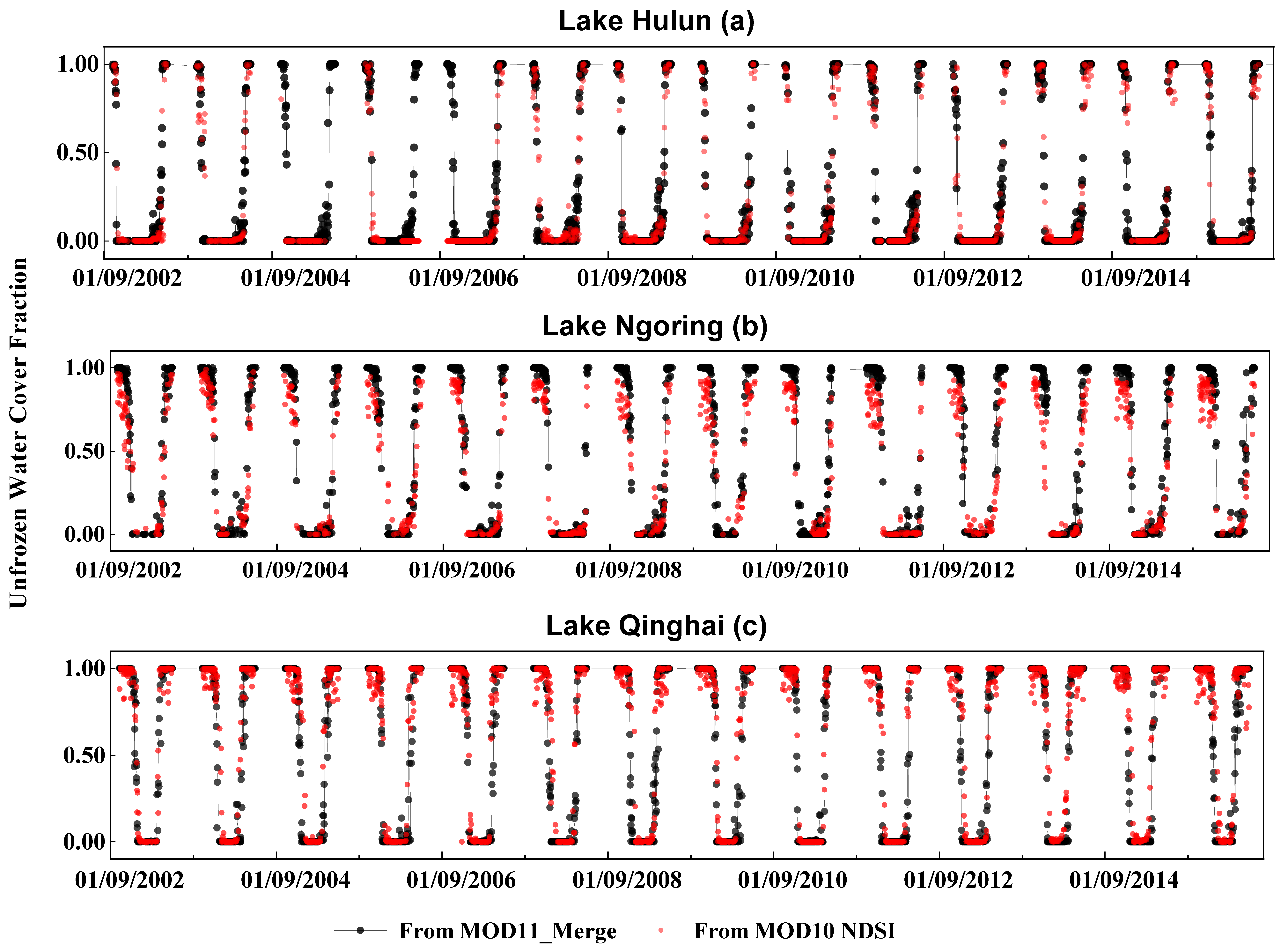
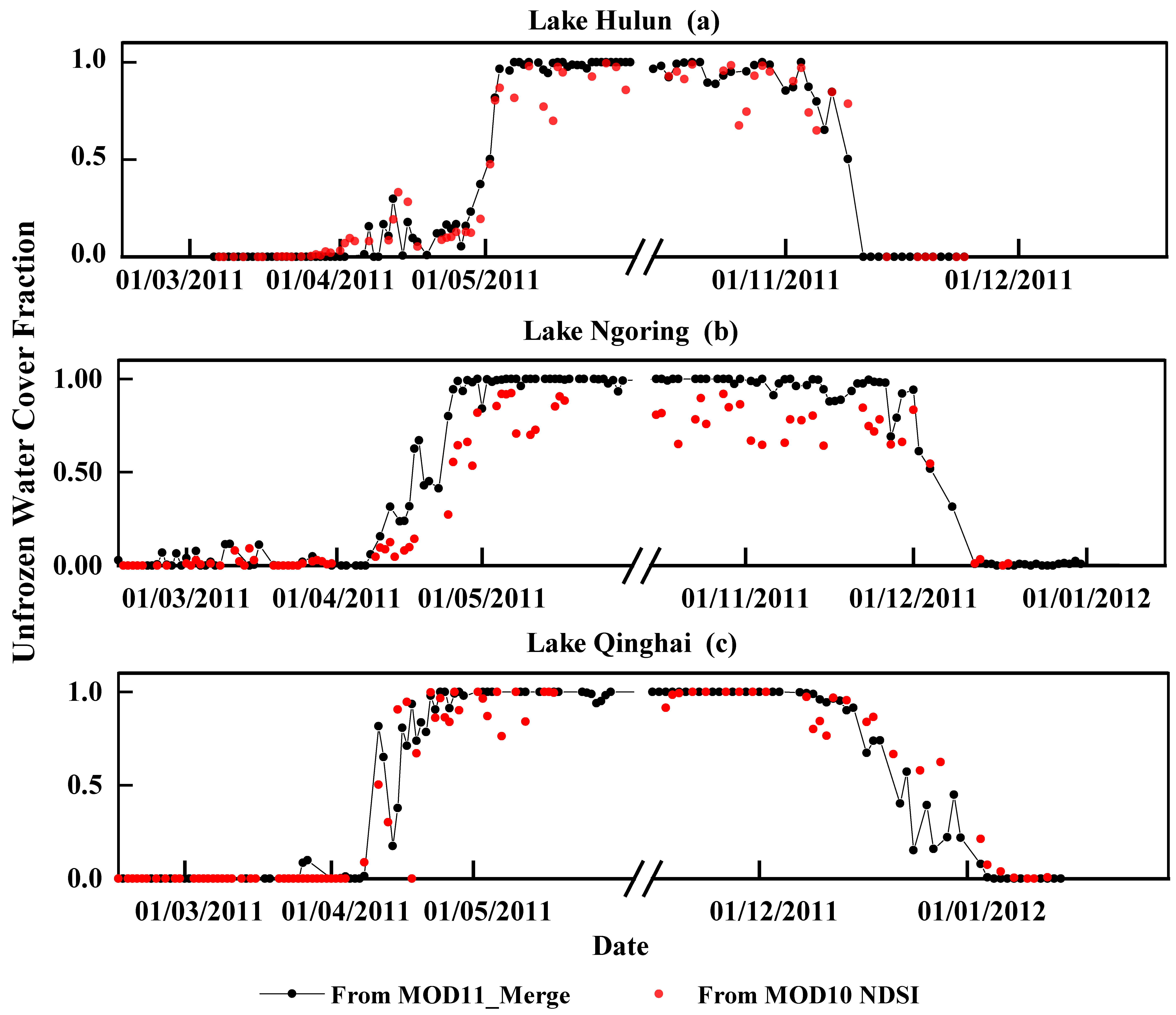
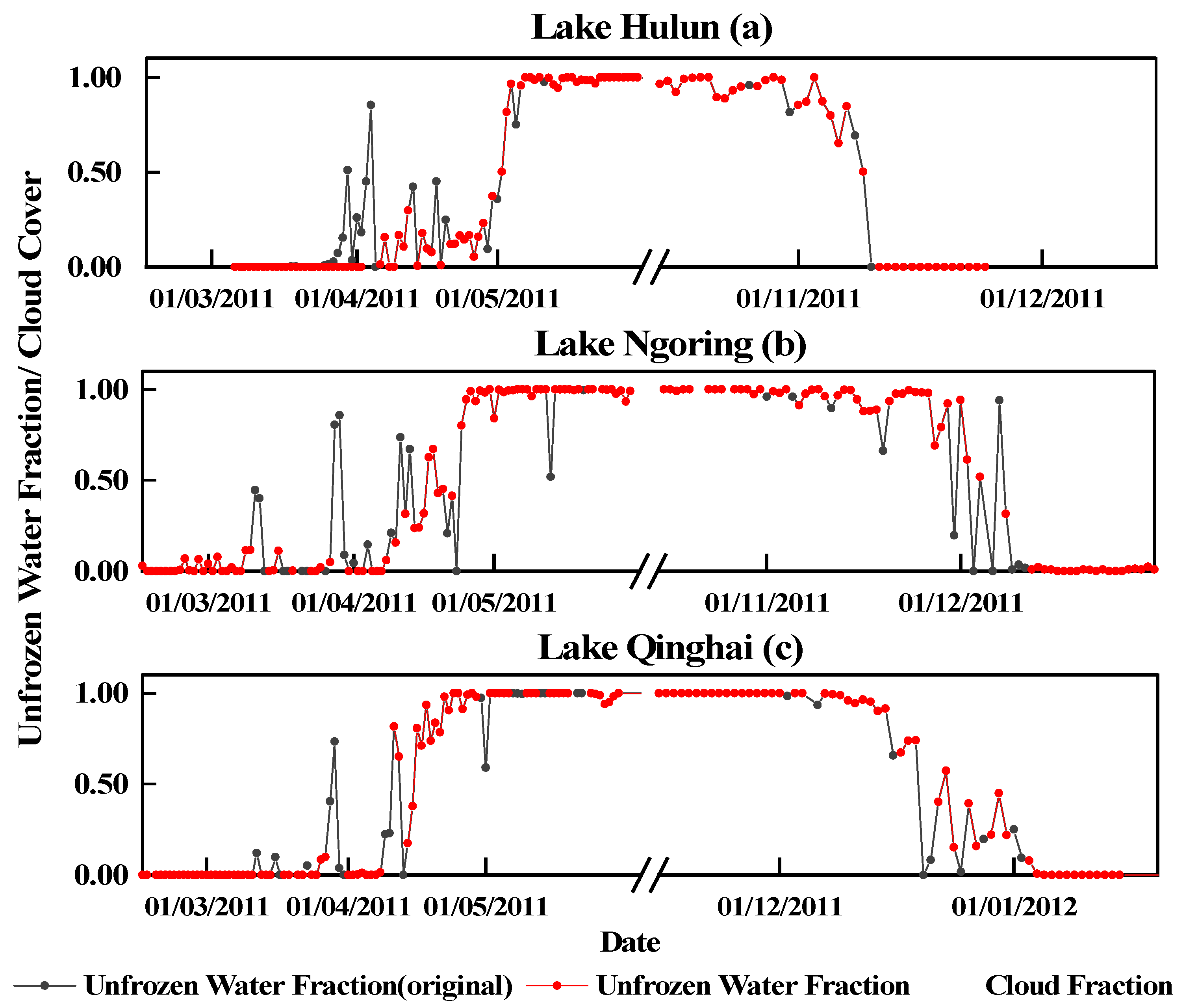
4.2. Comparison of the Unfrozen Water Cover Fraction with Other Datasets

The performance of the unfrozen water cover fraction obtained from MOD11_Merge daily images was compared with that from MODIS daily snow products, MODIS daily reflectance products, and Landsat images. These products have previously proven their ability to extract lake ice characteristics [18,21,23,56].

The unfrozen water cover fraction calculation and the outlier removal method (Section 3.2) were applied to the MODIS daily snow cover products. As shown in Figure 5 and Figure 6, the unfrozen water cover fraction obtained from MOD11_Merge was overall consistent with that of the MODIS snow cover product, with values of R² larger than 0.70 during the freeze-up pattern and 0.89 during the break-up pattern (

Table 3. The bias, SD, RMSE, and R² for the comparison of unfrozen water cover fraction between the MOD11_Merge and MODIS snow product data.

	Freeze-up Season (October–December)			Break-up Season (March–May)
	Lake Qinghai	Lake Ngoring	Lake Hulun	Lake Qinghai	Lake Ngoring	Lake Hulun
Bias	−0.05	0.15	0.00	0.04	0.18	0.05
SD	0.21	0.12	0.28	0.18	0.20	0.13
RMSE	0.22	0.19	0.28	0.18	0.29	0.14
R2	0.72	0.87	0.80	0.91	0.89	0.95

). Compared with the freeze-up patterns, the break-up patterns in MOD11_Merge and MODIS snow cover product showed higher agreement, with R² values of 0.912, 0.889, and 0.948, respectively. The freeze-up pattern in MOD11_Merge and MODIS snow cover in Lake Qinghai had a lower R², bias, and RMSE than the other two lakes, with values of 0.72, 0.22, and −0.55, respectively. This may be due to the thin ice or initial ice information, which was not easily detectable, especially in large lakes [14,15].

The visual inspections of lake ice under clear-day conditions from the MODIS daily reflectance products and Landsat images were further used to evaluate the water/ice cover information. The unfrozen water cover fraction in the phases of break-up process was consistent with MODIS reflectance products, MODIS snow products, and MOD11_Merge temperature images, as shown in the Supplementary Materials, Figures S2–S4. This consistency was notably seen in the developed and final phases of ice cover than in the initial phase, especially in smaller Lake Ngoring (Supplementary Materials, Figure S4). When compared with Landsat images with a high resolution of 30 m, thin ice or fast ice at the lakeshores was difficult to detect from the MODIS products, either from snow products and temperature products, as shown in the Supplementary Materials, Figures S5–S7. The misclassification of thin ice was possibly caused by the lower temperature resulting from undetected cloud cover in the MODIS temperature products [23].

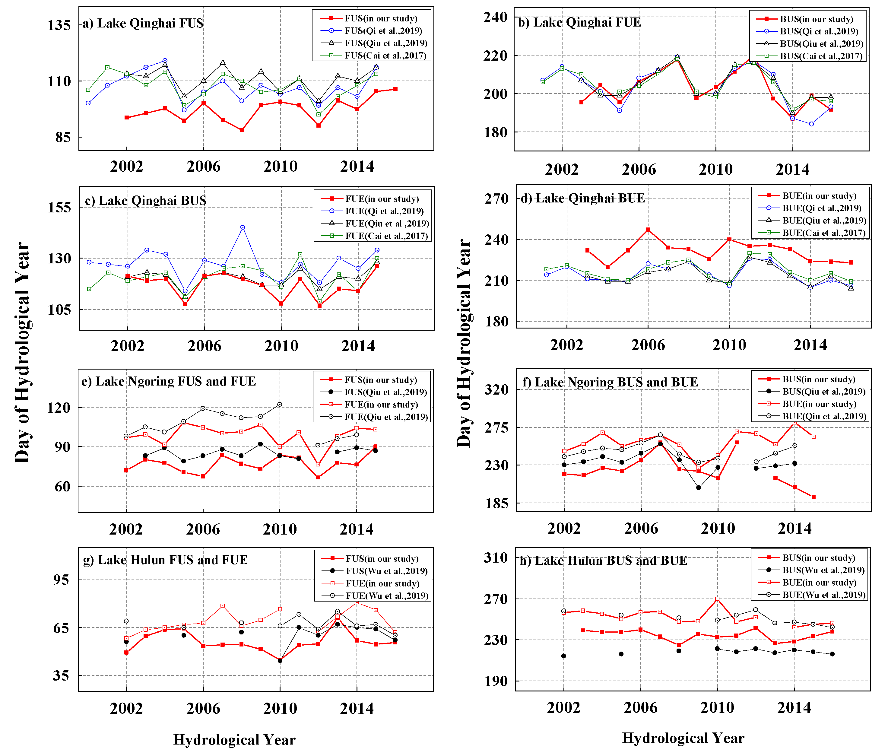
4.3. Comparison of Derived Lake Ice Phenology with other Lake Ice Datasets

The lake ice phenology was extracted from the temporal pattern of unfrozen water cover fraction by characterizing the water/ice transition process (as shown in Supplementary, Figure S1). The extracted ice phenology dates of Lake Qinghai, Lake Ngoring, and Lake Hulun were then compared with published lake ice datasets including microwave and optical satellite sensors, as listed in

Table 4. The data sources and the durations of other publishing lake ice phenology datasets.

Lake Name	Data Source and Reference	Duration
Lake Hulun	MODIS reflectance product [43]	2002–2016
Lake Ngoring	MODIS snow product [23]	2002–2015
	AMSR-E/2 [57]	2000–2016
Lake Qinghai	SSM/I [15]	2002–2015
	MODIS snow product [23]	1979–2016
	AMSR-E/2 [57]	2000–2016
	MODIS reflectance product [19]	2000–2016

. As shown in Figure 7a–d, the annual variation of ice phenology in Lake Qinghai from the proposed method was consistent with other datasets, with an R² of 0.90 when compared with MODIS snow products [56], an R² of 0.87 when compared with MODIS reflectance data [19], and with an R² of 0.80 when compared with passive microwave data [15].

The trends of break-up dates obtained from MOD11_Merge data had a high consistency with those of other MODIS products, less with passive microwave data, especially in Lake Qinghai, as shown in

Table 5. Trends of the freeze-up and break-up dates in our study and in other studies.

Trend (Days/10yr)	In Our Study				In Other Studies				Data Source
	FUS	FUE	BUS	BUE	FUS	FUE	BUS	BUE
Lake Qinghai	6.31	4.65	−4.82	−4.69	−4.09	−0.92	−8.63	−2.85	[19]
					−1.52	1.65	−3.96	−2.15	[57]
					−3.12	1.93	−5.94	−1.32	[15]
					4.00	4.90	−5.00	−0.70	[23]
Lake Ngoring	5.10	−1.69	−2.46	9.59	2.60	−4.76	−9.10	−4.14	[57]
					2.50	-	-	−0.20	[23]
Lake Hulun	0.10	15.80	−3.73	5.02	4.21	−1.76	2.16	−9.09	[43]

. However, the trends of freeze-up dates showed inconsistencies. For example, the trend of FUS in Lake Qinghai was −4.09 days/10 yr, while it was 4.00 days/10 yr from Cai, Y. et al. [15] and 6.31 days/10 yr in our study. This inconsistency could potentially be attributed to several factors, such as misclassification of the thin ice at the initial phase of freeze-up period, inhomogeneous definitions of lake ice phenology in different studies, and the coarser spatial resolution of the passive microwave data [13,14].

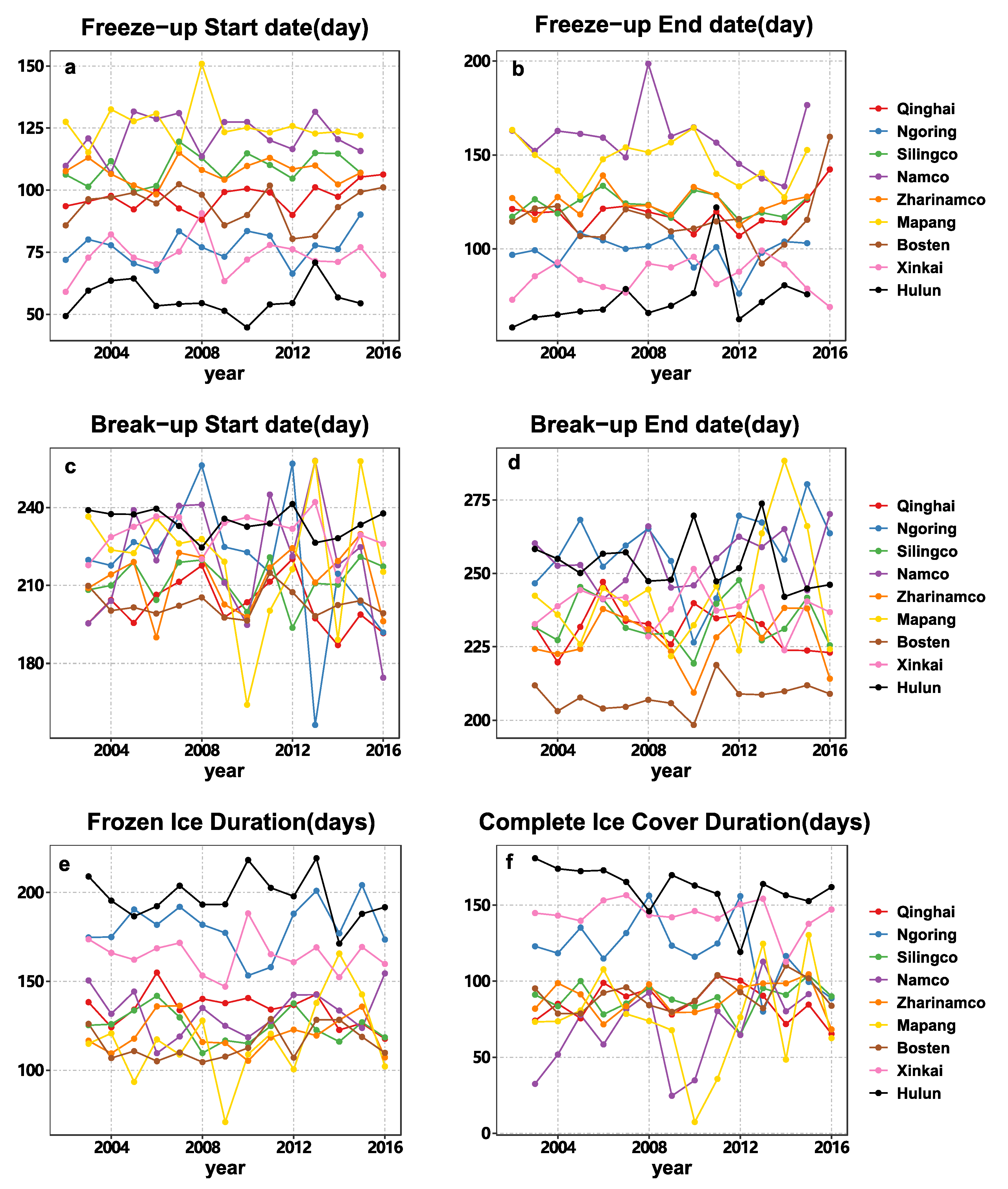
4.4. Interannual Variability in Lake Ice Phenology

The extraction approach was applied to other lakes in different climatic regions of northern China. The temporal patterns and trends of ice phenology from 2002 to 2016 are shown in Figure 8 and

Table 6. The mean values and trends of lake ice phenology variables in all lakes.

Lake Name	FUS		FUE		BUS		BUE		FID		CID
	Mean Value (Day)	Trend (Days/10yr)	Mean Value (Day)	Trend (Days/10yr)	Mean Value (Day)	Trend (Days/10yr)	Mean Value (Day)	Trend (Days/10yr)	Mean Value (Day)	Trend (Days/10yr)	Mean Value (Day)	Trend (Days/10yr)
Lake Qinghai	97.67	6.31 **	119.65	4.65	201.13	−4.82	232.29	−4.69	135.45	−9.47	85.95	−2.77
Lake Ngoring	77.36	5.10	100.51	−1.69	221.31	−2.46	257.28	9.59	179.55	4.48	120.67	−22.94 *
Lake Silingco	108.55	5.30	123.87	−1.19	211.09	1.55	231.24	−1.00	125.11	−6.30	89.78	2.75
Lake Namco	120.65	3.34	159.59	−8.21	220.45	−1.48	254.03	6.93	132.69	4.08	77.73	32.70 *
Lake Zharinamco	107.86	0.09	124.19	−0.24	215.54	3.29	228.08	1.78	118.10	1.69	87.61	3.54
Lake Mapang	124.35	−2.65	148.89	−7.98	223.05	−5.16	241.06	15.86	116.12	18.51	73.72	2.82
Lake Bosten	96.30	−0.59	114.62	4.56	201.84	−0.88	208.24	3.54	110.34	6.69	89.70	8.10
Lake Xinkai	72.79	0.60	85.47	0.98	231.82	−0.53	238.79	−1.36	165.67	−4.53	144.10	−6.55
Lake Hulun	54.46	0.10	68.71	15.80 *	234.78	−3.73	250.99	−5.02	194.41	−5.12	163.42	−19.53 **

** represents the Statistical significance at the 0.05 level, and * represents the Statistical significance at the 0.1 level.

. In general, shallower lakes had earlier freeze-up dates than deeper lakes (Figure 8): FUS and FUE in Lake Hulun (mean depth 5 m) were 69 and 91 days earlier than in Lake Namco (mean depth 43 m). The trends in ice phenology variables among the Tibetan lakes during the period 2002–2016 revealed a tendency towards delayed FUS dates, with the highest value being 6.31 days/10 yr (p < 0.05) in Lake Qinghai and the lowest value being 0.09 days/10 yr in Lake Zharinamco. Trends of BUE dates were also positive in all lakes on the Tibetan Plateau except Lake Silingco and Lake Qinghai, with insignificant BUE trends of −1.00 days/10 yr and −4.69 days/10 yr, respectively. Compared to the lakes on the Tibetan Plateau, the break-up starts and end dates rapidly shifted to be earlier in Lake Hulun (−3.73 days/10 yr; −5.02 days/10 yr). The short length of the data record (15 years) may be one of reasons that trends have no significance.

5. Discussion

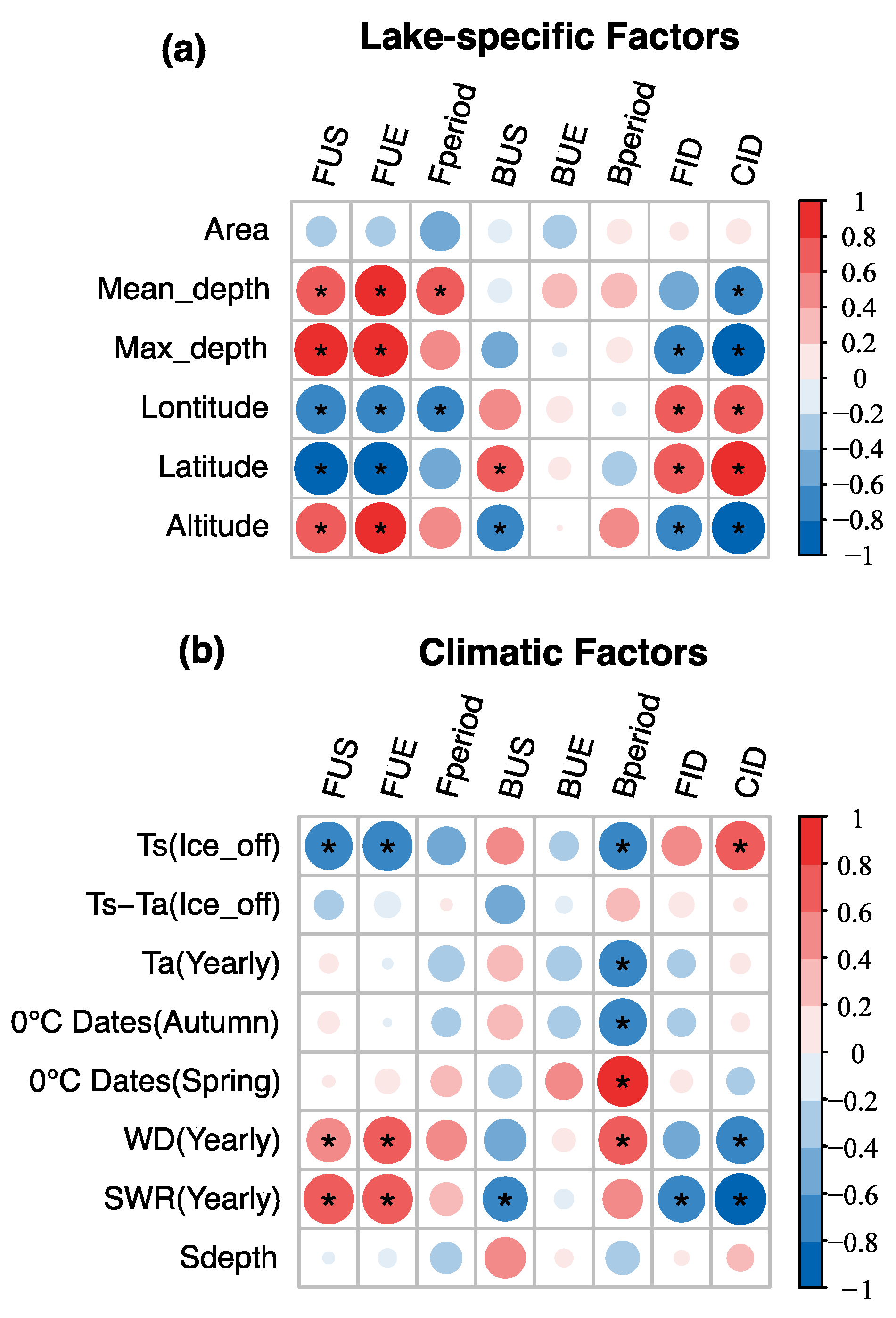
5.1. Factors Influencing Lake Ice Phenology

The growth and decay of lake ice cover are governed by thermodynamic interactions between atmosphere–water–ice interfaces and are affected by climatic and lake-specific factors. The major climatic factors controlling the heat exchange with the atmosphere are air temperature, solar radiation, precipitation, and wind speed [5,8,10]. Lake-specific factors, such as lake morphometry (depth, area, and volume) and location (longitude, latitude, and altitude), determine heat storage in lakes and additionally affect lake ice formation [58]. To assess how lake-specific and climatic factors contribute to the freeze-up and break-up patterns and the changes in the ice cover duration, the correlations between ice phenology time series extracted in our study and possible influencing factors including lake specific factors and major climatic factors were analyzed. The climatic variables, including air temperature, wind speed, solar radiation, and snow depth, were obtained from 2002 to 2016 from the China Meteorological Administration dataset based on the nearest weather station. The mean values of the lake surface water temperature (LSWT) data during the ice-off period used in our study were calculated based on the MOD11_merge dataset. Our LSWT results showed high consistency with publicly available satellite-derived LSWT products, such as the Arclake [59] and LSWT datasets from AVHRR [60], with R² values of 0.91 and 0.93, respectively. The other climatic factors were obtained from weather stations near the lakes.

As shown in Figure 9, the results suggest that climate factors strongly affected the break-up pattern, while lake-specific factors had a greater effect on the freeze-up pattern that agrees with previously published findings [61,62,63]. Deep high-altitude lakes showed later freeze-up dates and shorter ice cover durations, while shallower lakes located at high latitudes showed earlier freeze-ups and longer ice cover durations. The air temperature had a significant effect on the break-up date and the duration of the ice-covered period. The dates at which the air temperature reached 0 °C in the spring even had a high R² value (0.81) for the break-up periods. The LSWT had a more obvious impact on the freeze-up date (freeze-up day and rate) and CID than on the break-up pattern.

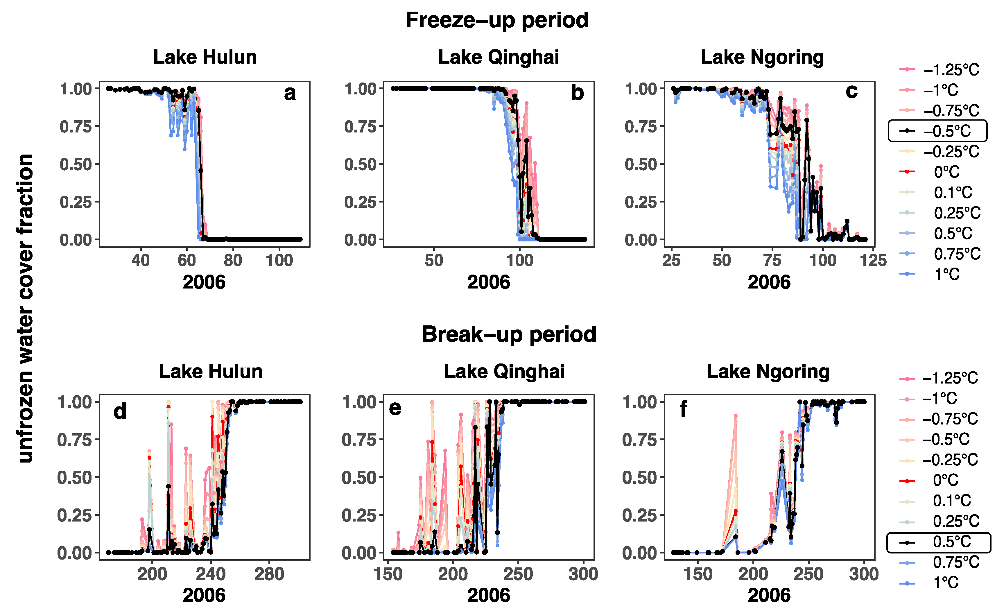
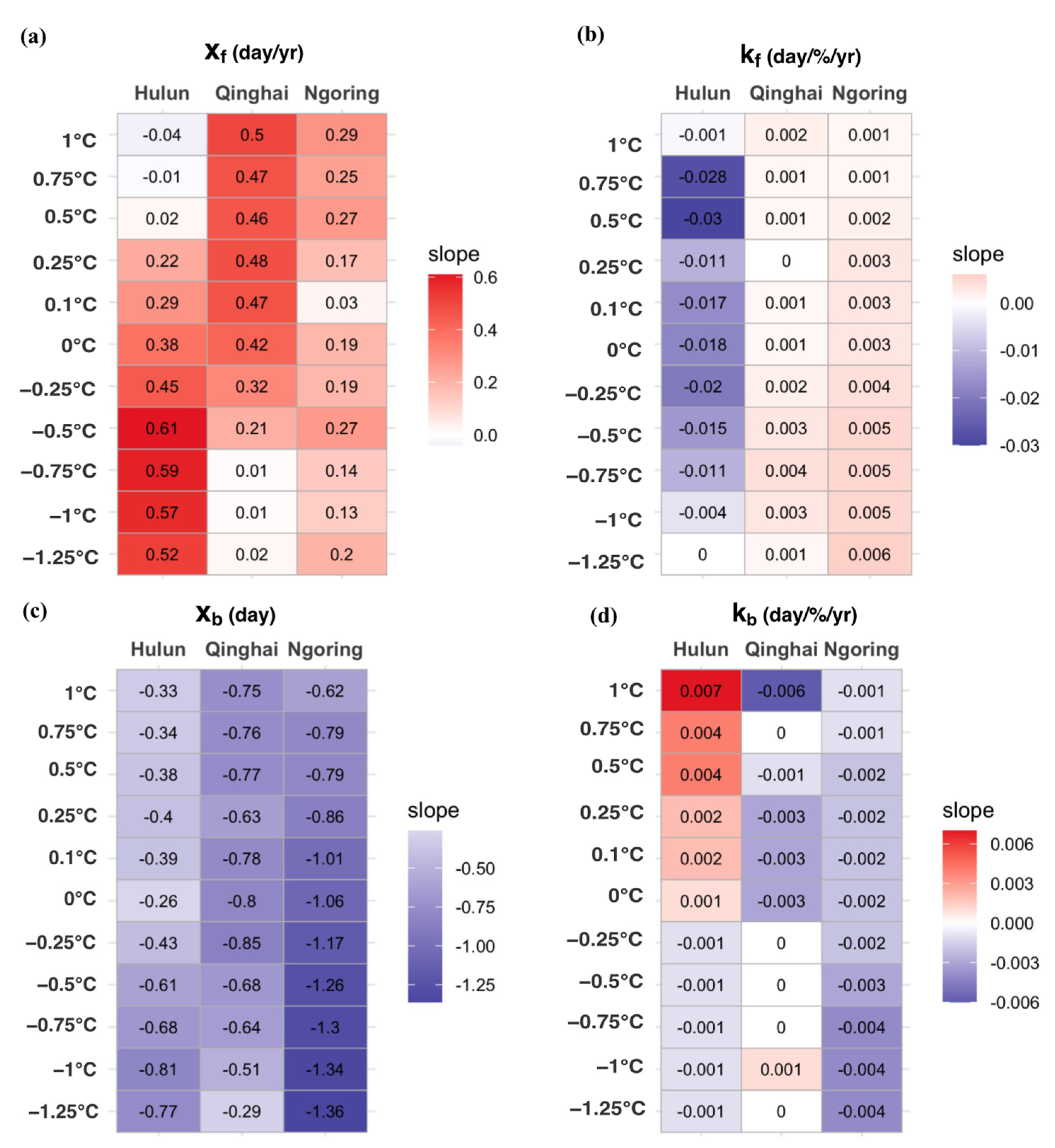
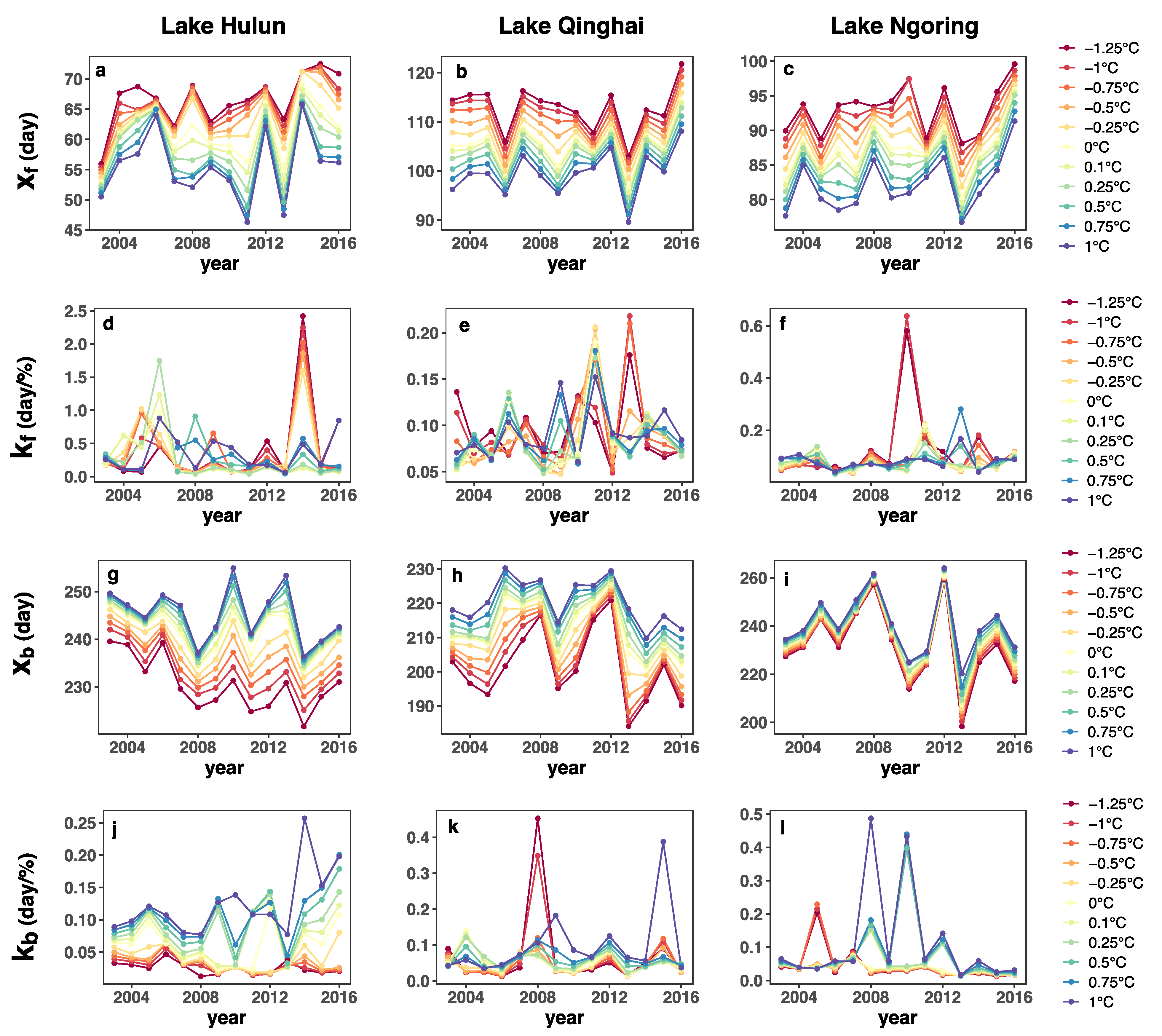
5.2. Sensitivity Analysis of Classification for Water/ice Status Pixels

The sensitivity of the water/ice classification status to the threshold value was evaluated by a lake ice phenology extraction under different freezing and melting temperatures, which was varied in 0.25 °C intervals within the range from −1.25 °C to 1 °C. Figure 10 shows the temporal pattern of the ice fitting variables ($x_f$ and $k_f$, and $x_b$ and $k_b$) among the three lakes, under different freezing and melting temperature settings. Consistent fluctuations were found in the interannual variabilities in $x_f$ and $x_b$. The variabilities in $k_f$ and $k_b$ were relatively stable except when the temperature threshold was too high or too low (Figure 11). As shown in Figure 10a–c, the freeze-up process occurred earlier when the freezing temperature was set higher. The temporal pattern of the unfrozen water cover fraction was stable and consistent when the freezing temperature was set between −0.75 °C and 0.5 °C. The break-up process showed relatively high variability in the initial phase, especially when the melting temperature was set lower than 0 °C (Figure 10d–f). This variability was possibly due to the melt-refreeze events captured when the temperature setting was too low, which were not representative of the starting point of the actual break-up process.

The trends of $x_f$ and $k_f$ were consistent when the temperature threshold varied between −0.75 °C and 0.5 °C (Figure 12a,c). The trends of $x_b$ performed consistently well under different temperature settings, while the trends of $k_b$ showed good consistency when the melting temperature was above 0 °C, possibly caused by the high fluctuations in the initial phase of the break-up process. These findings suggest that the trends of ice phenology are robust when the freezing temperature is set between −0.75 °C and 0.5 °C and the melting temperature is set above 0 °C.

The temperature classification applied for the water/ice status should consider the lake surface situation in the freeze-up pattern and break-up pattern, respectively. The freezing temperature can be influenced by several factors. Water salinity can decrease the freezing temperature and delay ice formation [64]. Moreover, the ice pixel temperature can be influenced by the bubble contents, impurities, and fracture patterns of ice surfaces [65]. Ice break-up starts after the ice/snow surface is warmed up to the melting point [63]. Melting snow, snow-ice and black ice have different reflectance values [66,67]. Furthermore, the day and night melt-freeze events produce meltwater on the ice surface before the ice cover break-up completely. To consider these uncertainties, and the physical basis of ice cover, we determined the classified pixel as “ice” when its temperature was lower than −0.5 °C and classified the pixel as “water” when its temperature was higher than 0.5°C.

5.3. The Advantages and Limitations of the Method

The proposed algorithm of the ice phenology extraction possesses several distinct advantages for wide-scale application on seasonal ice-covered lakes. An important qualitative advance is to scale the transition period between the open water and the ice-covered stage by a parameterized function of time (Equation (3)). The scaling-based method has been proven to be robust to outliers and can be applied to lakes with varying morphometry. Additionally, the characterization of the seasonal ice phenology can be extended beyond the binary ice-on/ice-off events by the direct assessment of the “partial ice cover” duration. The latter characteristic is crucial for understanding the lake response to ice cover formation, especially in medium to large lakes. During ice formation in autumn, the length of the transitional period determines the rate of cooling across the entire water column: a faster formation of the complete ice cover allows more heat to be stored in the near-bottom part of the lake, affecting the water–ice heat fluxes throughout the entire ice-covered period and the ice thickness [63,68,69]. In turn, the length of the transition period to the ice-free state in spring causes long-lasting effects on the vertical thermal stratification in the following summer and thereby affects crucial lake water quality characteristics, such as the dissolved oxygen content [63,69]. Both autumn and spring transitional periods are the results of interaction between the air–lake heat transport, the available solar radiation, and the heat storage in the lake water column. Therefore, they serve as sensitive indicators of the regional response to global climate change. When applied to long-term remote sensing observations, the proposed approach would allow tracing the climatically driven effects on non-linear interactions between various components of the surface heat balance during autumn and spring. The proposed approach also builds on the strengths of the MODIS daily temperature products. The Terra and Aqua daily combination from four observations with a time step of 4 to 7 hours demonstrates the effectiveness in reducing the cloud contamination while retaining the essential spatial information. The automatic temperature-based algorithm was also shown the ability to correctly extract ice phenology on different lake types concerning potential influences caused by salinity, morphometry, and geographic location.

The limitations of the proposed algorithm are intrinsic to remote sensing products. Firstly, thin ice cover is formed when lake surface temperature approaches the freezing temperature, but it may be repeatedly destroyed during windy periods with prolonged fluctuation of the surface temperature around 0 °C [63,69]. Therefore, thin ice is difficult to detect using temperature-based methods. Secondly, the severe cloud contaminations caused inevitable data gaps, although the data availability was improved by Terra and Aqua daily combination in our study. Additionally, MODIS-derived LSWT was revealed to have a negative bias compared with in situ observations, especially during the daytime. The negative bias could potentially have been caused by several things, including undetected cloud cover [46,51], cool skin, and warm layer effects [70,71,72]. Furthermore, Terra and Aqua daily combination could cause additional uncertainties due to ignoring the diurnal variation of lake surface temperature. Finally, although the spatial resolution of 1 km from MODIS temperature products is relatively high compared to other remote sensing products, like AMSR-E, it is still relatively coarse for phenology studies on lakes with horizontal dimensions smaller than several kilometers, especially located at high elevations or in areas covered by persistent snow cover. Progress in phenology observations on small lakes could be made by obtaining sub-kilometer spatial resolutions while retaining the sub-daily temporal resolution of data.

6. Conclusions

In this study, we developed a new automatic method to characterize lake ice phenology using MODIS daily temperature products from 2002 to 2016 by parameterizing the temporal pattern of the water/ice transition process. Based on this method, the ice phenology of nine seasonal ice-covered lakes in different climate regions was evaluated. The results showed that Lake Qinghai had the most obvious trend towards delayed freeze-up start date (FUS) (6.31 days/10 yr) among the lakes of the Tibetan plateau, and Lake Hulun the most obvious tendency towards earlier break-up start and end dates (BUS and BUE), with change rates of -3.73 days/10 yr and −5.02 days/10 yr, respectively. The proposed method has two major advantages, making it robust and applicable: (i) it avoids any lake-specific or empirical thresholds, allowing the effective treatment of data gaps caused by atmospheric conditions, and (ii) it uses a time-dependent parameterized function to characterize the water/ice transition process, making it possible to trace the ice phenology on a more detailed level than traditional binary classification. The algorithm could provide data support for the correct interpretation of the global-scale climate change effects on lake ice phenology: apart from the general shortening of the ice-cover period, the interplay between atmospheric warming and seasonally available shortwave solar radiation may produce significant changes in the duration of transitional—partially ice-covered—periods with important consequences for air-lake interactions and internal lake mixing.

References

1. Adrian, R.; O’Reilly, C.M.; Zagarese, H.; Baines, S.B.; Hessen, D.O.; Keller, W.; Livingstone, D.M.; Sommaruga, R.; Straile, D.; van Donk, E.; et al. Lakes as sentinels of climate change. Limnol. Oceanogr. 2009, 54, 2283–2297. [Google Scholar] [CrossRef] [PubMed]
2. Magnuson, J.J.; Robertson, D.; Benson, B.J.; Wynne, R.H.; Livingstone, D.M.; Arai, T.; Assel, R.A.; Barry, R.G.; Card, V.; Kuusisto, E.; et al. Historical Trends in Lake and River Ice Cover in the Northern Hemisphere. Science 2000, 289, 1743–1746. [Google Scholar] [CrossRef] [PubMed] [Green Version]
3. Sharma, S.; Blagrave, K.; Magnuson, J.J.; O’Reilly, C.M.; Oliver, S.; Batt, R.D.; Magee, M.; Straile, D.; Weyhenmeyer, G.A.; Winslow, L.; et al. Widespread loss of lake ice around the Northern Hemisphere in a warming world. Nat. Clim. Chang. 2019, 9, 227–231. [Google Scholar] [CrossRef]
4. Beyene, M.T.; Jain, S.; Gupta, R.C. Linear-Circular Statistical Modeling of Lake Ice-Out Dates. Water Resour. Res. 2018, 54, 7841–7858. [Google Scholar] [CrossRef]
5. Benson, B.J.; Magnuson, J.J.; Jensen, O.P.; Card, V.M.; Hodgkins, G.; Korhonen, J.; Livingstone, D.M.; Stewart, K.M.; Weyhenmeyer, G.A.; Granin, N.G. Extreme events, trends, and variability in Northern Hemisphere lake-ice phenology (1855–2005). Clim. Chang. 2011, 112, 299–323. [Google Scholar] [CrossRef]
6. Weyhenmeyer, G.A.; Livingstone, D.M.; Meili, M.; Jensen, O.P.J.P.; Benson, B.J.; Magnuson, J.J. Large geographical differences in the sensitivity of ice-covered lakes and rivers in the Northern Hemisphere to temperature changes. Glob. Chang. Biol. 2010, 17, 268–275. [Google Scholar] [CrossRef]
7. Weyhenmeyer, G.A.; Meili, M.; Livingstone, D.M. Nonlinear temperature response of lake ice breakup. Geophys. Res. Lett. 2004, 31, 07203. [Google Scholar] [CrossRef] [Green Version]
8. Jensen, O.P.; Benson, B.J.; Magnuson, J.J.; Card, V.M.; Futter, M.; Soranno, P.; Stewart, K.M. Spatial analysis of ice phenology trends across the Laurentian Great Lakes region during a recent warming period. Limnol. Oceanogr. 2007, 52, 2013–2026. [Google Scholar] [CrossRef] [Green Version]
9. Warne, C.P.K.; McCann, K.S.; Rooney, N.; Cazelles, K.; Guzzo, M.M. Geography and Morphology Affect the Ice Duration Dynamics of Northern Hemisphere Lakes Worldwide. Geophys. Res. Lett. 2020, 47, 087953. [Google Scholar] [CrossRef]
10. Brown, L.C.; Duguay, C.R. The response and role of ice cover in lake-climate interactions. Prog. Phys. Geogr. Earth Environ. 2010, 34, 671–704. [Google Scholar] [CrossRef]
11. IGOS. Integrated Global Observing Strategy Cryosphere Theme Report—For the Monitoring of our Environment from Space and from Earth; World Meteorological Organization: Geneva, Switzerland, 2007; 100p. [Google Scholar]
12. Duguay, C.R.; Bernier, M.; Gauthier, Y.; Kouraev, A. Remote Sensing of lake and river ice. In Remote Sensing of the Cryosphere; Tedesco, M., Ed.; Wiley Blackwell: Hoboken, NJ, USA, 2015; pp. 273–306. [Google Scholar] [CrossRef]
13. Kang, K.-K.; Duguay, C.R.; Howell, S.E.L. Estimating ice phenology on large northern lakes from AMSR-E: Algorithm development and application to Great Bear Lake and Great Slave Lake, Canada. Cryosphere 2012, 6, 235–254. [Google Scholar] [CrossRef] [Green Version]
14. Du, J.; Kimball, J.S.; Duguay, C.; Kim, Y.; Watts, J.D. Satellite microwave assessment of Northern Hemisphere lake ice phenology from 2002 to 2015. Cryosphere 2017, 11, 47–63. [Google Scholar] [CrossRef] [Green Version]
15. Cai, Y.; Ke, C.-Q.; Duan, Z. Monitoring ice variations in Qinghai Lake from 1979 to 2016 using passive microwave remote sensing data. Sci. Total. Environ. 2017, 607-608, 120–131. [Google Scholar] [CrossRef]
16. Ke, C.-Q.; Tao, A.-Q.; Jin, X. Variability in the ice phenology of Nam Co Lake in central Tibet from scanning multichannel microwave radiometer and special sensor microwave/imager: 1978 to 2013. J. Appl. Remote Sens. 2013, 7, 073477. [Google Scholar] [CrossRef]
17. Che, T.; Li, X.; Dai, L. Monitoring freeze-up and break-up dates of Northern Hemisphere big lakes using passive microwave remote sensing data. In Proceedings of the 2011 IEEE International Geoscience and Remote Sensing Symposium, Vancouver, BC, Canada, 24–29 July 2011; IEEE: Piscataway, NJ, USA, 2011; pp. 3191–3193. [Google Scholar]
18. Zhang, S.; Pavelsky, T.M. Remote Sensing of Lake Ice Phenology across a Range of Lakes Sizes, ME, USA. Remote Sens. 2019, 11, 1718. [Google Scholar] [CrossRef] [Green Version]
19. Qi, M.; Yao, X.; Li, X.; Duan, H.; Gao, Y.; Liu, J. Spatiotemporal characteristics of Qinghai Lake ice phenology between 2000 and 2016. J. Geogr. Sci. 2019, 29, 115–130. [Google Scholar] [CrossRef] [Green Version]
20. Šmejkalová, T.; Edwards, M.E.; Dash, J. Arctic lakes show strong decadal trend in earlier spring ice-out. Sci. Rep. 2016, 6, 38449. [Google Scholar] [CrossRef]
21. Wu, Y.; Duguay, C.R.; Xu, L. Assessment of machine learning classifiers for global lake ice cover mapping from MODIS TOA reflectance data. Remote Sens. Environ. 2021, 253, 112206. [Google Scholar] [CrossRef]
22. Kropáček, J.; Maussion, F.; Chen, F.; Hoerz, S.; Hochschild, V. Analysis of ice phenology of lakes on the Tibetan Plateau from MODIS data. Cryosphere 2013, 7, 287–301. [Google Scholar] [CrossRef] [Green Version]
23. Cai, Y.; Ke, C.; Li, X.; Zhang, G.; Duan, Z.; Lee, H. Variations of Lake Ice Phenology on the Tibetan Plateau From 2001 to 2017 Based on MODIS Data. J. Geophys. Res. Atmos. 2019, 124, 825–843. [Google Scholar] [CrossRef]
24. Murfitt, J.; Brown, L.C. Lake ice and temperature trends for Ontario and Manitoba: 2001 to 2014. Hydrol. Process. 2017, 31, 3596–3609. [Google Scholar] [CrossRef]
25. Pepin, N.; Deng, H.; Zhang, H.; Zhang, F.; Kang, S.; Yao, T. An Examination of Temperature Trends at High Elevations Across the Tibetan Plateau: The Use of MODIS LST to Understand Patterns of Elevation-Dependent Warming. J. Geophys. Res. Atmos. 2019, 124, 5738–5756. [Google Scholar] [CrossRef] [Green Version]
26. Gao, Y.; Xie, H.; Yao, T.; Xue, C. Integrated assessment on multi-temporal and multi-sensor combinations for reducing cloud obscuration of MODIS snow cover products of the Pacific Northwest USA. Remote Sens. Environ. 2010, 114, 1662–1675. [Google Scholar] [CrossRef]
27. Gafurov, A.; Bárdossy, A. Cloud removal methodology from MODIS snow cover product. Hydrol. Earth Syst. Sci. 2009, 13, 1361–1373. [Google Scholar] [CrossRef] [Green Version]
28. López-Burgos, V.; Gupta, H.V.; Clark, M.P. Reducing cloud obscuration of MODIS snow cover area products by combining spatio-temporal techniques with a probability of snow approach. Hydrol. Earth Syst. Sci. 2013, 17, 1809–1823. [Google Scholar] [CrossRef] [Green Version]
29. Li, X.; Jing, Y.; Shen, H.; Zhang, L. The recent developments in cloud removal approaches of MODIS snow cover product. Hydrol. Earth Syst. Sci. 2019, 23, 2401–2416. [Google Scholar] [CrossRef] [Green Version]
30. Hall, D.K.; Riggs, G.A.; DiGirolamo, N.E.; Román, M.O. Evaluation of MODIS and VIIRS cloud-gap-filled snow-cover products for production of an Earth science data record. Hydrol. Earth Syst. Sci. 2019, 23, 5227–5241. [Google Scholar] [CrossRef] [Green Version]
31. Parajka, J.; Bloschl, G. Spatio-temporal combination of MODIS images - potential for snow cover mapping. Water Resour. Res. 2008, 44. [Google Scholar] [CrossRef]
32. Xie, H.; Wang, X.; Liang, T. Development and assessment of combined Terra and Aqua snow cover products in Colorado Plateau, USA and northern Xinjiang, China. J. Appl. Remote Sens. 2009, 3, 033559. [Google Scholar] [CrossRef]
33. Wang, X.; Xie, H. New methods for studying the spatiotemporal variation of snow cover based on combination products of MODIS Terra and Aqua. J. Hydrol. 2009, 371, 192–200. [Google Scholar] [CrossRef]
34. Latifovic, R.; Pouliot, D. Analysis of climate change impacts on lake ice phenology in Canada using the historical satellite data record. Remote Sens. Environ. 2007, 106, 492–507. [Google Scholar] [CrossRef]
35. Nonaka, T.; Matsunaga, T.; Hoyano, A. Estimating ice breakup dates on Eurasian lakes using water temperature trends and threshold surface temperatures derived from MODIS data. Int. J. Remote Sens. 2007, 28, 2163–2179. [Google Scholar] [CrossRef]
36. Weber, H.; Riffler, M.; Nõges, T.; Wunderle, S. Lake ice phenology from AVHRR data for European lakes: An automated two-step extraction method. Remote Sens. Environ. 2016, 174, 329–340. [Google Scholar] [CrossRef]
37. Zhang, X.; Friedl, M.A.; Schaaf, C.B.; Strahler, A.H.; Hodges, J.C.F.; Gao, F.; Reed, B.C.; Huete, A. Monitoring vegetation phenology using MODIS. Remote Sens. Environ. 2003, 84, 471–475. [Google Scholar] [CrossRef]
38. Julien, Y.; Sobrino, J.A. Comparison of cloud-reconstruction methods for time series of composite NDVI data. Remote Sens. Environ. 2010, 114, 618–625. [Google Scholar] [CrossRef]
39. Beck, P.S.; Atzberger, C.; Høgda, K.A.; Johansen, B.; Skidmore, A. Improved monitoring of vegetation dynamics at very high latitudes: A new method using MODIS NDVI. Remote Sens. Environ. 2006, 100, 321–334. [Google Scholar] [CrossRef]
40. Liu, R.; Shang, R.; Liu, Y.; Lu, X. Global evaluation of gap-filling approaches for seasonal NDVI with considering vegetation growth trajectory, protection of key point, noise resistance and curve stability. Remote Sens. Environ. 2017, 189, 164–179. [Google Scholar] [CrossRef] [Green Version]
41. Melaas, E.K.; Friedl, M.A.; Zhu, Z. Detecting interannual variation in deciduous broadleaf forest phenology using Landsat TM/ETM+ data. Remote Sens. Environ. 2013, 132, 176–185. [Google Scholar] [CrossRef]
42. Li, Z.; Lyu, S.; Wen, L.; Zhao, L.; Ao, Y.; Meng, X. Study of freeze-thaw cycle and key radiation transfer parameters in a Tibetan Plateau lake using LAKE2.0 model and field observations. J. Glaciol. 2021, 67, 91–106. [Google Scholar] [CrossRef]
43. Wu, Q.; Li, C.; Sun, B.; Shi, X.; Zhao, S.; Han, Z. Change of ice phenology in the Hulun Lake from 1986 to 2017. Prog. Geogr. 2019, 38, 1933–1943. [Google Scholar] [CrossRef]
44. Suming, W. Records of Chinese Lakes; Science Press: Beijing, China, 1998. (In Chinese) [Google Scholar]
45. Wan, Z.; Dozier, J. A generalized split-window algorithm for retrieving land-surface temperature from space. IEEE Trans. Geosci. Remote Sens. 1996, 34, 892–905. [Google Scholar] [CrossRef] [Green Version]
46. Wan, Z. New refinements and validation of the MODIS Land-Surface Temperature/Emissivity products. Remote Sens. Environ. 2008, 112, 59–74. [Google Scholar] [CrossRef]
47. Hall, D.K.; Riggs, G.A. Accuracy assessment of the MODIS snow products. Hydrol. Process. 2007, 21, 1534–1547. [Google Scholar] [CrossRef]
48. Riggs, G.A.; Hall, D.K.; Román, M.O. Modis Snow Products User Guide for Collection 6.1 (c6.1). 2019. Available online: https://modis-snow-ice.gsfc.nasa.gov/uploads/C6_MODIS_Snow_User_Guide.pdf (accessed on 15 January 2021).
49. Cao, L.; Zhu, Y.; Tang, G.; Yuan, F.; Yan, Z. Climatic warming in China according to a homogenized data set from 2419 stations. Int. J. Clim. 2016, 36, 4384–4392. [Google Scholar] [CrossRef] [Green Version]
50. Zhang, G.; Yao, T.; Shum, C.K.; Yi, S.; Yang, K.; Xie, H.; Feng, W.; Bolch, T.; Wang, L.; Behrangi, A.; et al. Lake volume and groundwater storage variations in Tibetan Plateau’s endorheic basin. Geophys. Res. Lett. 2017, 44, 5550–5560. [Google Scholar] [CrossRef]
51. Zhang, X.; Wang, K.; Frassl, M.A.; Boehrer, B. Reconstructing Six Decades of Surface Temperatures at a Shallow Lake. Water 2020, 12, 405. [Google Scholar] [CrossRef] [Green Version]
52. Duguay, C.R.; Prowse, T.D.; Bonsal, B.R.; Brown, R.D.; Lacroix, M.P.; Ménard, P. Recent trends in Canadian lake ice cover. Hydrol. Process. 2006, 20, 781–801. [Google Scholar] [CrossRef]
53. Tjørve, K.M.; Tjorve, E. A proposed family of Unified models for sigmoidal growth. Ecol. Model. 2017, 359, 117–127. [Google Scholar] [CrossRef]
54. Villegas, D.; Aparicio, N.; Blanco, R.; Royo, C. Biomass Accumulation and Main Stem Elongation of Durum Wheat Grown under Mediterranean Conditions. Ann. Bot. 2001, 88, 617–627. [Google Scholar] [CrossRef] [Green Version]
55. White, K.; Pontius, J.; Schaberg, P. Remote sensing of spring phenology in northeastern forests: A comparison of methods, field metrics and sources of uncertainty. Remote Sens. Environ. 2014, 148, 97–107. [Google Scholar] [CrossRef]
56. Qiu, Y.; Xie, P.; Leppäranta, M.; Wang, X.; Lemmetyinen, J.; Lin, H.; Shi, L. MODIS-based Daily Lake Ice Extent and Coverage dataset for Tibetan Plateau. Big Earth Data 2019, 3, 170–185. [Google Scholar] [CrossRef]
57. Qiu, Y. Dataset of Microwave Brightness Temperature and the Freeze-Thaw Process for Medium-to-Large Lakes in the High Asia Region (2002–2016); National Tibetan Plateau Data Center: Beijing, China, 2018. [Google Scholar]
58. Jeffries, M.O.; Morris, K.; Kozlenko, N. Ice characteristics and processes, and remote sensing of frozen rivers and lakes. In Remote Sensing in Northern Hydrology: Measuring Environmental Change; American Geophysical Union (AGU): Washington, DC, USA, 2005; pp. 63–90. [Google Scholar]
59. Maccallum, S.N.; Merchant, C.J. Surface water temperature observations of large lakes by optimal estimation. Can. J. Remote Sens. 2012, 38, 25–45. [Google Scholar] [CrossRef]
60. Liu, B.; Wan, W.; Xie, H.; Li, H.; Zhu, S.; Zhang, G.; Wen, L.; Hong, Y. A long-term dataset of lake surface water temperature over the Tibetan Plateau derived from AVHRR 1981–2015. Sci. Data 2019, 6, 48. [Google Scholar] [CrossRef] [PubMed]
61. Bernhardt, J.; Engelhardt, C.; Kirillin, G.; Matschullat, J. Lake ice phenology in Berlin-Brandenburg from 1947–2007: Observations and model hindcasts. Clim. Chang. 2011, 112, 791–817. [Google Scholar] [CrossRef]
62. Cai, Y.; Ke, C.-Q.; Yao, G.; Shen, X. MODIS-observed variations of lake ice phenology in Xinjiang, China. Clim. Chang. 2020, 158, 575–592. [Google Scholar] [CrossRef]
63. Kirillin, G.; Leppäranta, M.; Terzhevik, A.; Granin, N.; Bernhardt, J.; Engelhardt, C.; Efremova, T.; Golosov, S.; Palshin, N.; Sherstyankin, P.; et al. Physics of seasonally ice-covered lakes: A review. Aquat. Sci. 2012, 74, 659–682. [Google Scholar] [CrossRef]
64. Stepanenko, V.; Repina, I.A.; Ganbat, G.; Davaa, G. Numerical Simulation of Ice Cover of Saline Lakes. Izv. Atmospheric Ocean. Phys. 2019, 55, 129–138. [Google Scholar] [CrossRef]
65. Mullen, P.C.; Warren, S.G. Theory of the optical properties of lake ice. J. Geophys. Res. Space Phys. 1988, 93, 8403–8414. [Google Scholar] [CrossRef]
66. Bolsenga, S.J. Spectral Reflectances of Snow and Fresh-Water Ice from 340 Through 1100 nm. J. Glaciol. 1983, 29, 296–305. [Google Scholar] [CrossRef] [Green Version]
67. Maslanik, J.; Barry, R. Lake ice formation and breakup as an indicator of climate change: Potential for monitoring using remote sensing techniques. In The Influence of Climate Change and Climatic Variability on the Hydrologic Regime and Water Resources; IAHS Publication Press: Wallingford, UK, 1987; Volume 168, pp. 153–161. [Google Scholar]
68. Huang, W.; Zhang, J.; Leppäranta, M.; Li, Z.; Cheng, B.; Lin, Z. Thermal structure and water-ice heat transfer in a shallow ice-covered thermokarst lake in central Qinghai-Tibet Plateau. J. Hydrol. 2019, 578, 124122. [Google Scholar] [CrossRef]
69. Leppäranta, M. Freezing of Lakes; Springer Science and Business Media LLC: Berlin, Germany, 2014; pp. 11–50. [Google Scholar]
70. Crosman, E.T.; Horel, J.D. MODIS-derived surface temperature of the Great Salt Lake. Remote Sens. Environ. 2009, 113, 73–81. [Google Scholar] [CrossRef]
71. Liu, G.; Ou, W.; Zhang, Y.; Wu, T.; Zhu, G.; Shi, K.; Qin, B. Validating and Mapping Surface Water Temperatures in Lake Taihu: Results from MODIS Land Surface Temperature Products. IEEE J. Sel. Top. Appl. Earth Obs. Remote Sens. 2015, 8, 1230–1244. [Google Scholar] [CrossRef]
72. Sima, S.; Ahmadalipour, A.; Tajrishy, M. Mapping surface temperature in a hyper-saline lake and investigating the effect of temperature distribution on the lake evaporation. Remote Sens. Environ. 2013, 136, 374–385. [Google Scholar] [CrossRef]
Figure 1. The locations of the selected lakes. (A) Lake Qinghai; (B) Lake Ngoring; (C) Lake Silingco; (D) Lake Namco; (E) Lake Zharinamco; (F) Lake Mapang; (G) Lake Bosten; (H) Lake Xinkai; and (I) Lake Hulun.
Remotesensing 13 02711 g001
Figure 2. Flowchart of the automated detection of lake ice phenology from MODIS daily temperature products.
Remotesensing 13 02711 g002
Figure 3. Extraction of the unfrozen water cover fraction values in Lake Hulun (a), Lake Ngoring (b), and Lake Qinghai (c). The gray columns represent the cloud cover. The blue dot line represents the unfrozen water cover fraction without outlier removal, and the red dot line represents the unfrozen water cover fraction after outliner removal.
Remotesensing 13 02711 g003
Figure 4. Schematic representation of the logistic function. The solid circles represent the midpoints of the freeze-up and break-up period. The shaded areas are the freeze-up and break-up periods.
Remotesensing 13 02711 g004
Figure 5. Time series of unfrozen water cover fractions in Lake Hulun (a), Lake Ngoring (b), and Lake Qinghai (c) from 2002 to 2016 calculated from MOD11_Merge temperature images and MODIS snow product data (referred MODIS NDSI as the label).
Remotesensing 13 02711 g005
Figure 6. Comparison of unfrozen water cover fractions in Lake Hulun, Lake Ngoring, and Lake Qinghai from MOD11_Merge temperature images and MODIS snow product data, taking the year 2011 as an example.
Remotesensing 13 02711 g006
Figure 7. Comparison of lake ice phenology dates between our study (the right y-axis) and other studies (the left y-axis) in Lake Qinghai (ad), Lake Ngoring (ef), and Lake Hulun (gh). The lake ice phenology dates extracted in our study are shown as dotted lines. The y-axis is the day of the hydrological year (1 September is referred to as Day 1 in our study).
Remotesensing 13 02711 g007
Figure 8. Temporal changes in lake ice phenology variables from 2002 to 2016. (a) Freeze-up day; (b) freeze-up rate; (c) break-up day; (d) break-up rate; (e) duration of frozen ice cover; and (f) duration of completed ice cover.
Remotesensing 13 02711 g008
Figure 9. Correlation maps between lake ice phenology variables and climatic (a) and lake-specific factors (b). Red indicates a positive correlation, and blue indicates a negative correlation. The size of the circle represents the absolute value of the correlation coefficient. The * represents significance at a confidence level of 0.1. Ts (ice_off) is the lake water surface temperature during the ice-off period, and Ta (yearly) is the annual mean air temperature. The 0 °C dates (autumn/spring) represent the dates at when air temperature reached 0 °C in the autumn/spring. WD (yearly) and SWR (yearly) represent the annual mean wind speed and shortwave solar radiation, respectively.
Remotesensing 13 02711 g009
Figure 10. The temporal pattern of the unfrozen water cover fraction was calculated using different freezing and melting temperatures of pixel settings. (ac) Freeze-up pattern, and (df) break-up pattern. The colored lines indicate the unfrozen water cover fraction indices based on the corresponding freezing (melting) temperatures of pixels.
Remotesensing 13 02711 g010
Figure 11. The temporal variations in ice phenology variables during the period 2002–2016, extracted from the unfrozen water cover fraction calculated by different freezing and melting temperatures of pixel settings. The colored lines indicate the time series of four variables obtained from the unfrozen water cover fraction indices based on the corresponding freezing (melting) temperature of pixels. The first row presents the time series of x f among the three lakes (ac), and the second row presents the time series of k f (df), and the third row presents the time series of x b (gi), and the fourth row presents the time series of k b (jl).
Remotesensing 13 02711 g011
Figure 12. (ad) The ice phenology variable trends under different freezing and melting temperatures of pixel settings. The x-axis is the lake, and the y-axis is the trend of the unfrozen water cover fraction. The red and blue tiles indicate positive trends and negative trends, respectively.
Remotesensing 13 02711 g012