Project Report

Monitoring Greenhouse Gases from Space

by Hartmut Boesch 1,2,*, Yi Liu 3, Johanna Tamminen 4, Dongxu Yang 3, Paul I. Palmer 5,6, Hannakaisa Lindqvist 4, Zhaonan Cai 3, Ke Che 3, Antonio Di Noia 1, Liang Feng 5,6, Janne Hakkarainen 4, Iolanda Ialongo 4, Nikoleta Kalaitzi 1, Tomi Karppinen 7, Rigel Kivi 7, Ella Kivimäki 4, Robert J. Parker 1,2, Simon Preval 1, Jing Wang 3, Alex J. Webb 1,2, Lu Yao 3 and Huilin Chen 8add Show full author list remove Hide full author list
1
School of Physics and Astronomy, University of Leicester, Leicester LE1 7RH, UK
2
National Centre for Earth Observation NCEO, University of Leicester, Leicester LE1 7RH, UK
3
Key Laboratory of the Middle Atmosphere and Global Environmental Observation (LAGEO), & Carbon Neutrality Research Center (CNRC), Institute of Atmospheric Physics, Chinese Academy of Sciences, Beijing 100029, China
4
Finnish Meteorological Institute, 00560 Helsinki, Finland
5
Finnish Meteorological Institute, 99600 Sodankylä, Finland
6
School of GeoSciences, University of Edinburgh, Edinburgh EH9 3FF, UK
7
National Centre for Earth Observation NCEO, University of Edinburgh, Edinburgh EH3 9FF, UK
8
Center for Isotope Research, University of Groningen, 9747 Groningen, The Netherlands
*
Author to whom correspondence should be addressed.
Remote Sens. 2021, 13(14), 2700; https://doi.org/10.3390/rs13142700
Submission received: 28 May 2021 / Revised: 2 July 2021 / Accepted: 2 July 2021 / Published: 8 July 2021
(This article belongs to the Special Issue ESA - NRSCC Cooperation Dragon 4 Final Results)

Abstract

:
The increase in atmospheric greenhouse gas concentrations of CO2 and CH4, due to human activities, is the main driver of the observed increase in surface temperature by more than 1 °C since the pre-industrial era. At the 2015 United Nations Climate Change Conference held in Paris, most nations agreed to reduce greenhouse gas emissions to limit the increase in global surface temperature to 1.5 °C. Satellite remote sensing of CO2 and CH4 is now well established thanks to missions such as NASA’s OCO-2 and the Japanese GOSAT missions, which have allowed us to build a long-term record of atmospheric GHG concentrations from space. They also give us a first glimpse into CO2 and CH4 enhancements related to anthropogenic emission, which helps to pave the way towards the future missions aimed at a Monitoring & Verification Support (MVS) capacity for the global stock take of the Paris agreement. China plays an important role for the global carbon budget as the largest source of anthropogenic carbon emissions but also as a region of increased carbon sequestration as a result of several reforestation projects. Over the last 10 years, a series of projects on mitigation of carbon emission has been started in China, including the development of the first Chinese greenhouse gas monitoring satellite mission, TanSat, which was successfully launched on 22 December 2016. Here, we summarise the results of a collaborative project between European and Chinese teams under the framework of the Dragon-4 programme of ESA and the Ministry of Science and Technology (MOST) to characterize and evaluate the datasets from the TanSat mission by retrieval intercomparisons and ground-based validation and to apply model comparisons and surface flux inversion methods to TanSat and other CO2 missions, with a focus on China.

1. Introduction

Carbon dioxide (CO2) is a major anthropogenic greenhouse gas. Its atmospheric concentration has increased from a pre-industrial value of about 280 parts per million (ppm) to more than 410 ppm as of 2020 [1]. This increase is the result of emissions from deforestation, land-use change, cement production, and fossil fuel combustion with fossil fuels becoming the dominant sources in the 1950s [2], and they are now representing more than 87% of all emissions [3]. Although there is broad consensus on the damaging consequences of the change in climate associated with further increasing atmospheric concentration of greenhouse gases, fossil fuel CO2 emissions have continued to increase in recent years with a growth of 1.2%/yr for the last decade (2010–2019). This continued increase in emissions is driven mainly by rapidly growing economies, with China being the largest national emitter of CO2, generating 28% of global emissions in 2019, which highlights the importance of this region for the global carbon budget.
In-situ networks provide a wealth of accurate CO2 concentration measurements at the surface. However, the sparse coverage of such networks is a major limitation, and large uncertainties remain about the magnitude, location, and durability of natural fluxes and anthropogenic emissions. Measurements of atmospheric CO2 from space can provide the required global coverage with the spatial and temporal resolution needed to improve our understanding of regional carbon fluxes, particularly for regions poorly sampled by surface networks, such as the Tropics or high latitudes.
Satellite-based measurements of the column-averaged dry air CO2 mole fraction (XCO2) in the near-infrared (NIR) and shortwave-infrared (SWIR) spectral range became possible in 2002 with the launch of the European Space Agency (ESA) SCanning Imaging Absorption SpectroMeter for Atmospheric CHartographY (SCIAMACHY) [3] on board ENVISAT. SCIAMACHY was operated until 2012 and has been continued by the Japanese Greenhouse Gases Observing Satellite (GOSAT) [4] and NASA’s Orbiting Carbon Observatory-2 (OCO-2) [5], launched in 2009 and 2014, respectively. In recent years, significant progress has been made in space-based CO2 measurements. XCO2, derived from GOSAT and OCO-2, has now reached an accuracy of better than 1 ppm when validated against measurements from the Total Carbon Column Observing Network (TCCON) [6,7,8,9,10], and they have contributed extensively to carbon flux studies [11,12,13,14].
China plays an important role for the global carbon budget as the largest source of anthropogenic carbon emissions [10] but also as a region of increased carbon sequestration as a result of several reforestation projects [15]. Over the last 10 years, a series of projects on mitigation of carbon emission has been started in China. This includes the first Chinese greenhouse gas monitoring satellite mission, TanSat, supported by the Ministry of Science and Technology of China (MOST), the Chinese Academy of Sciences (CAS), and the China Meteorological Administration (CMA).
The TanSat mission was successfully launched on 22 December 2016 into a sun-synchronous low Earth orbit (LEO) with an equator crossing time around 13:30 local time and started to acquire data operationally in March 2017 [16,17]. The TanSat satellite carries two instruments: the Atmospheric Carbon Dioxide Grating Spectrometer (ACGS) and the Cloud and Aerosol Polarimetry Imager (CAPI).
ACGS is a state-of-the-art hyperspectral grating spectrometer [18,19,20] that measures backscattered sunlight in three NIR/SWIR spectral bands: the oxygen (O2) A-band (758–778 nm with ~0.04 nm spectral resolution), the CO2 weak band (1594–1624 nm with ~0.125 nm spectral resolution) and the CO2 strong band (2042–2082 nm with ~0.16 nm spectral resolution). The key parameters are listed in Table 1.
CAPI is a wide field of view, multi-band imager that simultaneously measures radiance in five broad bands (365–408 nm, 660–685 nm, 862–877 nm, 1360–1390 nm, 1628–1654 nm) from the UV to NIR spectral range. To achieve more information on aerosol size, which impacts the wavelength dependence of aerosol optical properties, CAPI includes two polarization channels (660–685 nm and 1628–1654 nm) to measure the Stokes parameters [21].
TanSat measurements have a swath width of ~18 km across the satellite track and contain 9 footprints, each with a size of 2 km × 2 km in nadir [18,22]. TanSat operates in three measurement modes: nadir (ND), glint (GL), and target (TG). ND provides the routine measurements over land with the satellite flying in a rotation angle routine to track the principal plane (the principal plane is spanned by the vectors from the sun to the surface footprint and from the surface point to the observer). GL provides routine measurements over oceans, which are obtained by a consistent rotation motion as for ND. Nadir and glint mode alternate orbit-by-orbit, with the TanSat nadir ground track being typically between two tracks of the OCO-2 mission, which provides potential opportunities for combined usage of both datasets to increase coverage.
Here, we summarise the results of a collaborative project between European (UK and Finland) and Chinese teams under the framework of the Dragon-4 programme of ESA and the Ministry of Science and Technology (MOST). The goal of the project is to characterize and evaluate the datasets from the TanSat mission by retrieval intercomparisons and ground-based validation and to apply model comparisons and surface flux inversion methods to TanSat and other CO2 missions, with a focus on China. The project consists of two sub-projects, which are described in Section 2 and Section 3. The results of both projects are summarized in Section 4, followed by a conclusion (Section 5).

2. Project, Sub-Projects, EO and Other Data Utilisation

2.1. List of Sub-Projects and Teaming

The Dragon-4 project monitoring greenhouse gases from space consists of two co-aligned sub-projects:
  • Sub-Project 1: Monitoring greenhouse gases from space: retrieval algorithm development and CO2 and CH4 flux inversion
  • Sub-Project 2: Monitoring greenhouse gases from space: validation and uncertainties with focus in China and high latitudes
The project brings together researchers from the Institute of Atmospheric Physics from the Chinese Academy of Science, the Universities of Leicester and Edinburgh from the UK, and the Finnish Meteorological Institute. The lead investigators for the overall project are Hartmut Boesch (Europe) and Yi Liu (China). The teams involved in both sub-projects are detailed in Table 2.

2.2. Description and Summary Table of EO and Other Data Utilized

This project focusses on greenhouse gas monitoring satellites and we have made use of Level-1 and Level-2 data from the Chinese CO2 satellite TanSat, Level-2 data from the ESA Sentinel 5P mission, and Level-1 and Level-2 data from the ESA Third Party mission GOSAT (Table 3). We have also included Level-2 data from the NASA OCO-2 mission.

3. Subprojects’ Research and Approach:

3.1. Subproject 1: Monitoring Greenhouse Gases from Space: Retrieval Algorithm Development and CO2 and CH4 Flux Inversion

3.1.1. Research Aims

The overall aim of this subproject is to harmonize, characterize, and improve the retrieval and forward models used for the CO2 retrieval, for the TanSat missions, and to validate and interpret CO2 retrievals with the help of model calculation and CO2 data from other missions, such as GOSAT and OCO-2. We will also make steps toward using satellite data to constrain surface fluxes using inverse modelling to obtain sources and sink. The focus of this sub-project is global, but we will provide some emphasis on China.
The specific objectives of this sub-project are (1) to support the development of CO2 retrieval algorithms for TanSat by comparing retrieval results from different algorithms and by evaluating calibration uncertainties, for example, from radiometric calibration, (2) to evaluate global XCO2 datasets obtained from TanSat against model calculations, and (3) to conduct data assimilation experiments of satellite datasets to infer CO2 sources and sink information with a focus on China.

3.1.2. Research Approach

To achieve the objectives of this project, we make use of two different CO2 retrieval algorithms available within the project team and apply both to TanSat radiance measurements to retrieve the column averaged atmospheric CO2 dry air mole fraction (XCO2). This will then allow for the intercomparison and characterization of retrievals through validation with ground-based measurements, as well as comparison to global datasets from other missions. This work is linked with the sub-project on validation and uncertainties with a focus in China and high latitudes.
A focus of the analysis is given to the description of instrument parameters in the forward model of the retrieval, e.g., radiometric calibration, and we aim at investigating potential shortcomings in the available description for TanSat. Good knowledge of these parameters is critical for the accuracy of the retrieval, and by performing our retrieval tests, we will provide information that can help to improve the description of instrument and calibration parameters. This work is only possible thanks to the detailed instrument knowledge of the Chinese team.
Global CO2 datasets obtained from TanSat and other missions will be evaluated against state-of-the-art model calculations using the GEOS-Chem atmospheric transport model to assess if large scale spatial and temporal features are captured in both datasets. A final step will be to use the Ensemble Kalman filter method, combined with the GEOS-Chem model, to estimate and interpret surface fluxes from satellite CO2 data over China and globally.
The two retrieval algorithms used to generate XCO2 data from TanSat are IAPCAS and the UoL-FP. The Institute of Atmospheric Physics Carbon Dioxide Retrieval Algorithm for Satellite Remote Sensing (IAPCAS) is a full-physics retrieval algorithm that has been developed for space-based satellite measurement of greenhouse gases by TanSat and other satellites [8,22,23]. IAPCAS retrieves XCO2 together with aerosol, and other variables, using the Optimal Estimation Method (OEM) by iteratively analysing and optimizing the spectrum residual between the simulation and the satellite measurement. The University of Leicester (UoL-FP) algorithm is a full-physics retrieval algorithm, based on the Optimal Estimation method, originally developed for the NASA OCO mission but has since been applied to many other missions, including GOSAT and OCO-2 [24,25]. The UoL-FP and IAPCAS are based on the same retrieval principles (namely, Optimal Estimation), but they employ independent and different implementations of aerosols and radiative transfer solvers and use different retrieval setups.
We also use the GEOS-Chem model to allow model comparisons and to facilitate surface flux inversions. GEOS-Chem is an offline chemical transport model driven by GEOS-5 meteorological analysis form the Global Modelling and Assimilation Office (GMAO) Global Circulation Model. Atmospheric model simulations are forced by surface fluxes inferred from the data of atmospheric CO2 using an ensemble Kalman filter (EnkF) [26].

3.2. Subproject 2: Evaluation and Applications of TanSat Data in China and at High Latitudes

3.2.1. Research Aims

The accuracy requirements of satellite remote sensing of atmospheric composition and, in particular, greenhouse gases are challenging. The validation of the measurements is an essential part of the development of satellite remote sensing systems. In addition to ground-based validation, algorithm validation, including proper quantification of retrieval uncertainties, forms the basis for reliable satellite observations. Here, we focus on the recently launched Chinese TanSat satellite and aim to contribute to characterizing and improving the TanSat observations, and their uncertainty quantification, by validating the observations using ground-based reference observations. We use global ground-based observations and extend the validation, previously applied for Japanese GOSAT and NASA’s OCO-2 data, to TanSat. For more focused analysis we use reference observations in China and in Sodankylä high latitude site. As a demonstration of the applicability of the data for further research, we aim to analyse the potential of TanSat to detect emission areas from individual satellite overpasses.
The uncertainties of satellite observations of CO2 consist of the (i) observations themselves, such as noise and other systematic uncertainties and (ii) uncertainties in the retrieval step. The goal of the validation is to improve the retrievals and uncertainty characterization by analysing if any structures or correlations on potential reasons for uncertainties are detected. Typical validation analysis consists, thus, of aspects that have spatial and temporal dependencies, viewing geometry dependencies, swath position dependencies, and dependencies on main retrieval assumptions such as a priori profile shape, albedo and spectroscopy-related dependencies. Specific attention is commonly also put on analysing various aerosol or cloudiness conditions. Typically, satellite retrievals are improved in an iterative fashion, repeating validation and algorithm improvements repeatedly. Additional information is obtained if several retrieval algorithms are available—this allows separating observation dependent uncertainties and more retrieval algorithm dependent features. It may also allow some characterization of retrieval model uncertainties, which are commonly difficult to obtain. Here, we focus on the overall agreement with satellite and reference measurements to obtain, first, understanding on the agreement between well calibrated ground-based instruments and observations from TanSat. In addition, the TanSat product stability over time, and the seasonal variability of the bias, are evaluated.

3.2.2. Research Approach

We focus here on the validation of TanSat observations of vertical column integrated carbon dioxide, or more precisely, dry air mole fraction of carbon dioxide columns, denoted commonly as XCO2. It is well known that such column observations are best validated using similar vertically integrated column observations via Fourier Transform Spectrometer (FTS) ground-based observations. Global validation is obtained by using the TCCON network consisting of FTS instruments. Specific geographic focus is put to high latitudes. In China, validation campaigns have been conducted using EM27/SUN instruments in Beijing.
The Finnish Meteorological Institute has established, in Northern Finland, the Sodankylä-Pallas observation site (67°N, 27°E), which is widely used to validate/calibrate space-borne instruments. The measurements cover a great variety of both atmospheric and terrestrial parameters. The greenhouse gases are observed using in situ measurements of carbon dioxide and methane amounts as well as flux measurements. These observations are included in the ICOS-network. Column amounts of greenhouse gases are measured using the FTS instrument (Bruker 125 HR) which has been in operation at Sodankylä since 2009 and is part of the TCCON. The Sodankylä TCCON site [27] has participated on several satellite validation activities related to greenhouse gas observations of GOSAT, OCO-2, and Sentinel 5 Precursor TROPOMI (e.g., [28,29,30,31,32]).
From a validation point of view, the high latitude site in Sodankylä is very interesting: it covers a boreal/arctic environment combined with continuous measurements and good logistics. On the other hand, observation challenges include high solar zenith angles, clouds, and varying snow conditions.
The AirCore greenhouse gas profile measurement system at Sodankylä was established in September 2013. It is a sampling system, which is directly related to the World Meteorological Organization in situ trace gas measurement scales [33]. The AirCore method allows sampling in both the stratosphere and troposphere, and the sampling system has the potential to provide a ground-truth standard for comparison with measurements on board satellites and from ground-based FTS (e.g., [34,35,36,37,38]). The satellite and TCCON retrievals rely heavily on a priori profile shapes, and these retrieval assumptions can be compared to the observed reference profile measurements by using the AirCore observations.

4. Research Results and Conclusions

4.1. Subproject 1: Monitoring Greenhouse Gases from Space: Retrieval Algorithm Development and CO2 and CH4 Flux Inversion

4.1.1. Results

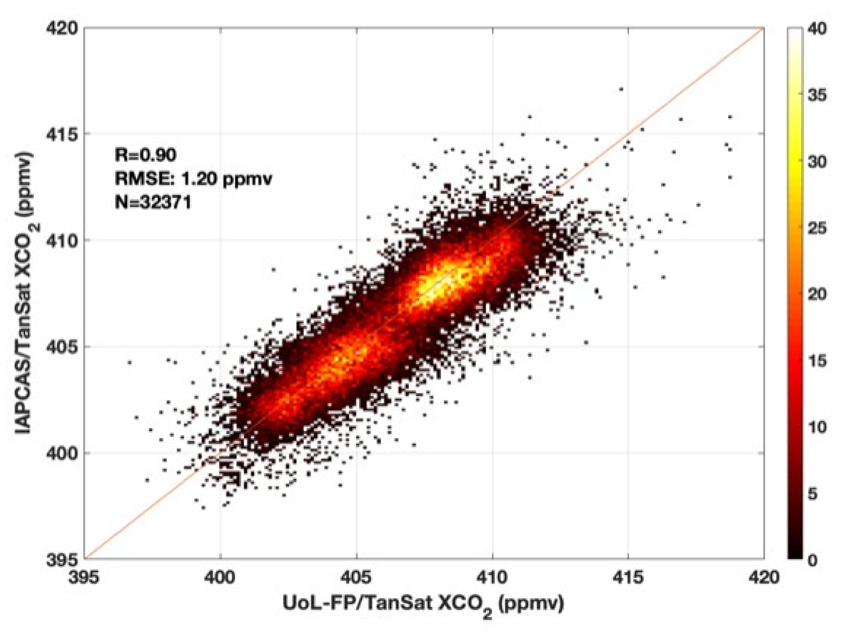
XCO2 Retrieval Algorithm Development and Intercomparison:

To infer XCO2 from the calibrated radiance spectra measured by a satellite a retrieval algorithm is used. This algorithm attempts at modelling the physics of the transfer of light through the atmosphere and of the instrument. Inadequacies in this description of the physics or in radiometric calibration can lead to biases in the retrieved XCO2.
To assess the radiometric performance of TanSat, we have analysed the solar calibration measurement of TanSat. The solar calibration measurements are direct measurements of the solar spectrum, and they are taken when TanSat flies over the ascending end of an orbit until almost in darkness. The solar measurements are without effects from the Earth’s atmosphere and surface and, thus, are well suited for tests of the radiometric calibration.
To analyse the solar calibration measurement, we have fitted a solar model to the measurements. This solar model consists of a solar line model (2016 version), created by G. C. Toon (2014) [39], and a continuum model that is obtained from SOLar SPECtrometer (SOLSPEC) measurements [40]. The analysis has been focused on the O2-A and weak CO2 band. We found that a considerable, but stable, pattern remained in the fitting residual, which is an indication of an imperfect calibration and which needs to be corrected to avoid errors in the XCO2 retrieval. The residual shows an oscillating nature, which we can describe by a Fourier series model of 8th order.
This radiometric correction model has been implemented in the UoL-FP retrieval algorithm, and we have created a 2-band XCO2 retrieval from TanSat that makes uses of the O2 A band and the weak CO2 band. We find that this approach leads to significant improvements, in the fitting residual from TanSat nadir spectra, by a factor of 4 in the O2 A band and by a factor of 2 in the weak CO2 band and accordingly reduces the difference to ground-based validation sites of the TCCON network, e.g., the RMSE against measurements from the site at Lamont (USA) decreases from 4.08 to 1.59 ppm.
To remove outliers, and to correct for small biases, introduced by an imperfect description of aerosol in the retrieval algorithm, for example, a data-driven quality control and bias correction method has been applied to the XCO2 retrieval. Parameters for quality filtering and bias correction are chosen based on the correlation of the RMSE of TanSat XCO2 against reference data given by the TCCON network. Threshold values for quality filtering are determined using a genetic algorithm and bias correction parameter are inferred from multi-linear regression. With this retrieval approach, we have retrieved all TanSat overpasses over TCCON sites. We find that, in total, 18% of all soundings pass the filter (64% of all cloud-free, converged retrievals) with a mean bias of 0.08 ppm and a RMSE of 1.47 ppm against TCCON data, which demonstrates that the radiometric correction has greatly improved the XCO2 retrieval. A detailed description of the UoL-FP retrieval from TanSat is given in Yang et al. (2020) [41].
This TanSat v2 dataset includes XCO2 from 15 months (March 2017–May 2018) of TanSat observations over land [42]. This approach for radiometric correction in the retrieval algorithm has also been implemented in the IAPCAS retrieval algorithm to generate a version 2 (v2) of the TanSat product. This version is a significant advance over version 1 (v1) which was based on a single (weak CO2) band [43]. A seasonal plot of the v2 TanSat data is given in Figure 1 covering the time period March 2017 to February 2018. The figure shows the expected seasonal variation of CO2 with a strong summer uptake by northern hemispheric forests and a peak-to-peak seasonal amplitude of +/− 3–4 ppm. The observed seasonal signal in the southern hemisphere is muted due to the much smaller amount of land masses. Gaps in coverage are the result of the quality filter applied. Enhancements in CO2 over emission regions, such as Eastern China, are less obvious in these seasonal maps. An example of observed CO2 enhancements in the TanSat dataset, related to emission sources, is given in in Section 4.2.1.
The TanSat v2 XCO2 data product can be obtained from the CASA TanSat data and science service (www.chinageoss.cn/tansat accessed January 2021). Information on measurement and retrieval quality, such as cloud clearing and post screening, is also provided in the data.
The IAPCAS and UoL-FP retrieval algorithms use a retrieval approach based on the Optimal Estimation method but both algorithms have been independently developed and their forward models and retrieval strategies are very different. Besides using different radiative transfer models and retrieval setups (retrieved parameters, a priori values), both algorithms differ in their treatment of aerosols. This is a key aspect, as it has been shown that scattering by already optically thin clouds or aerosols, if neglected, can introduce large errors in the CO2 retrieval [44]. Different schemes are used by different algorithms which will substantially reduce aerosol-induced errors. To reduce remaining errors in the retrieval, a quality filtering and post-retrieval bias correction are applied. They will have a significant impact on the quality of the final dataset and the filter, and bias correction by both algorithms differ, which is also an important aspect of the retrieval intercomparison. Residual errors will remain [9], which are hard to characterize other than by intercomparing results from different retrievals, which is the purpose of including both, the IAPCAS and the UoL-FP algorithm.
An intercomparison between the XCO2 retrievals from different algorithms will give insights into the robustness of the retrieval results. Initial comparisons, before including the radiometric correction term, did reveal a large spread between results from both retrieval algorithms [45]. The intercomparison of TanSat XCO2 retrievals between the two algorithms including the radiometric correction term for overpasses over TCCON sites with for solar zenith angle < 60° is given in Figure 2. In total, we find 32,271 cloud-free, quality-filtered soundings with a RMSE of 1.2 ppm, and a correlation coefficient of 0.9. The majority of the RMSE will be due to the measurement noise.

XCO2 Model Comparison and Surface Flux Inversions:

We run the global chemistry transport model GEOS-Chem v9.02 at a horizontal resolution of 4° × 5° using surface CO2 fluxes inferred from surface CO2 concentrations measured by the NOAA in-situ network, by using an Ensemble Kalman Filter (EnKF) [11]. To compare the GEOS-Chem model calculation to the TanSat XCO2 retrievals, we sample the model outputs at the TanSat observation location and time, and then convolve the resulting profiles with the averaging kernels from the TanSat XCO2 retrievals to calculate model XCO2 [46].
Figure 3a shows the cloud-free, quality-filtered global TanSat XCO2 retrievals between April 2017 and May 2018, gridded at 1° × 1° boxes, which are compared to the corresponding GEOS-Chem model simulation. (Figure 3b). The GEOS-Chem model output is sampled, according to the locations of the cloud-free, quality-filtered TanSat retrievals. The figure shows similar features in global XCO2 distributions in TanSat observations and model simulations. However, some noticeable differences are visible at tropical region (such India and the Northern Africa), which may be related to deficiency in our posterior CO2 flux estimates, due to coarse coverage by the current in-situ network [11], but biases in the satellite retrievals in this region might also contribute.
In a recent study, we used the GEOS-Chem atmospheric transport model and its counterpart Ensemble Kalman Filter inverse method to re-evaluate CO2 fluxes over China. Using newly available in situ CO2 mole fraction data from six sites across China and satellite data from the GOSAT and OCO-2 satellites from 2010 to 2016, we found a larger-than-expected carbon sink over southwest China [47]. Figure 4 shows the resulting net CO2 fluxes (natural + anthropogenic) over China, averaged for 2010 to 2016. We speculate the elevated land biosphere uptake is related to an extensive nationwide afforestation programme that has occurred over the past few decades [47]. This study is a powerful example of how data collected at a small number of additional sites can significantly revise our understanding of the carbon exchange, especially for otherwise poorly sampled regions, and how satellite observations will be a key tool to verify and monitor carbon fluxes.

4.1.2. Summary and Conclusions of Subproject 1

The TanSat XCO2 retrieval has been substantially improved with the inclusion of an additional radiometric correction term and this method has now been included in the IAPCAS and the UoL-FP algorithms. This leads not only to much improved spectral fits but also to a much improved comparisons against ground-based TCCON measurements with a mean bias of 0.08 ppm and a RMSE of 1.47 ppm. This improved performance is also reflected in a high level of agreement between the UoL-FP and the IAPCAS retrievals.
The improved version of the IAPCAS retrieval has now been used to generate a new global TanSat XCO2 datasets (v2) that is made publicly available. We have assessed this TanSat dataset against model calculations and we find good agreement with the spatial patterns in the global CO2 distribution but with larger differences in the Tropics. Using new in-situ data and satellite data from OCO-2 and GOSAT, we could demonstrate the power of atmospheric data to constrain CO2 surface fluxes over key regions, such as China. TanSat XCO2 data has much improved, thanks to this this and other projects, and a next step will be to use TanSat XCO2 data in top-down global carbon flux estimation so that TanSat data and associated surface fluxes can be used along-side OCO-2 and GOSAT.

4.2. Subproject 2: Evaluation and Applications of TanSat Data in China and at High Latitudes

4.2.1. Results

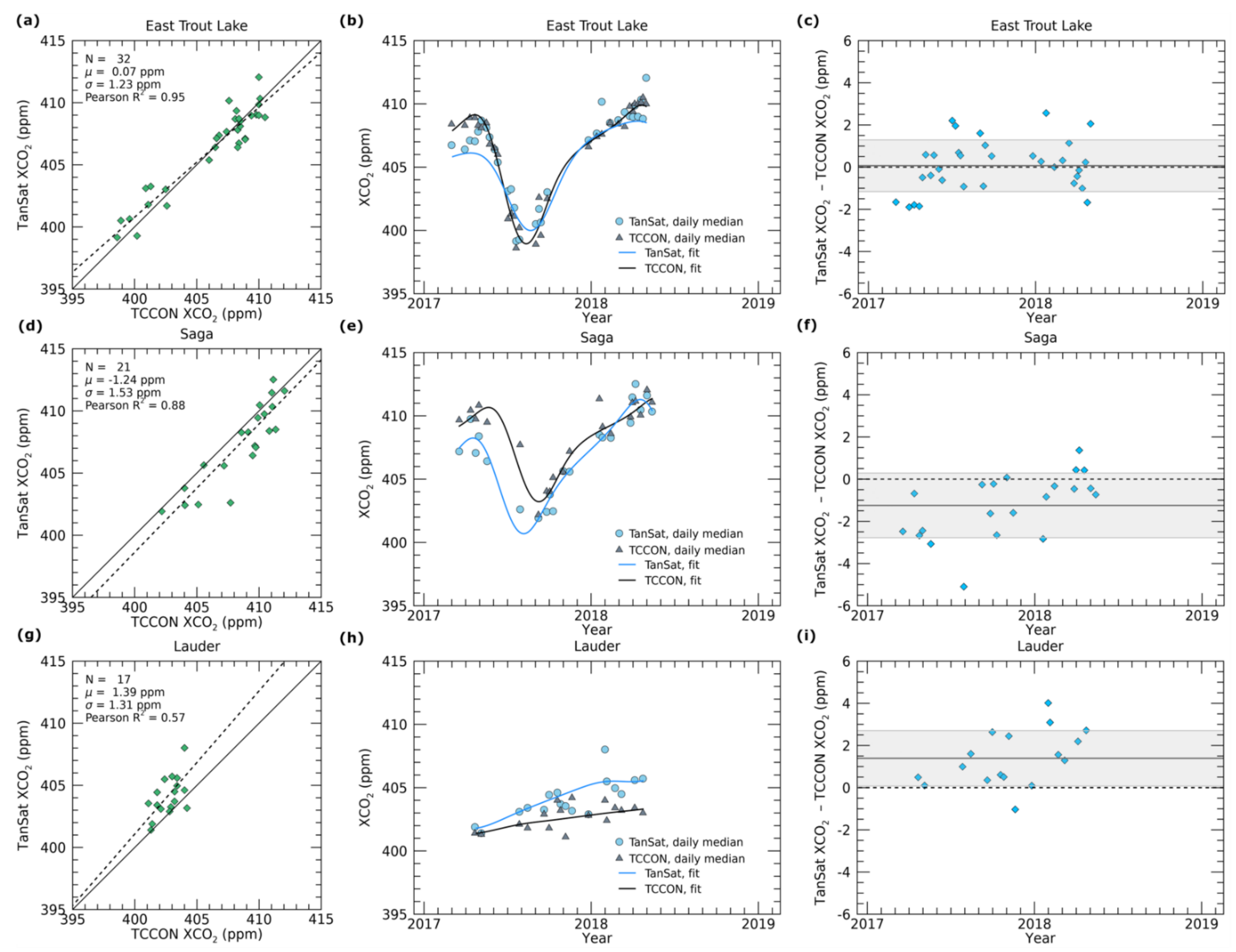
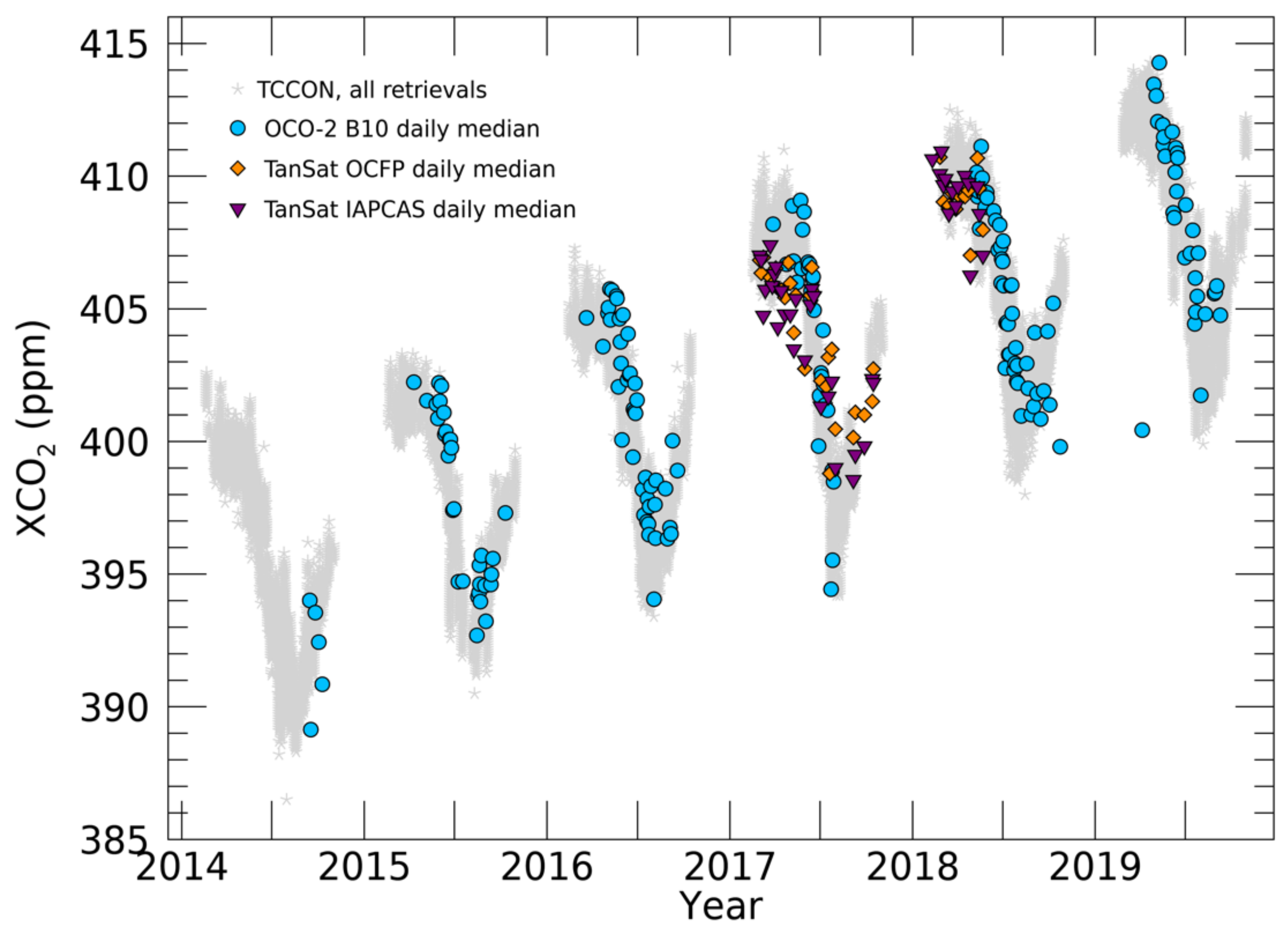
Evaluation against TCCON:

TanSat data were evaluated against the ground-based Fourier Transform Spectrometers that form the Total Carbon Column Observing Network [48]. The criteria for selecting the co-located retrievals were a maximum distance of 5 degrees in longitude and 2.5 degrees in latitude from the TCCON site. All same-day TCCON retrievals were considered for the determination of the daily median XCO2 that was compared to the median XCO2 of the TanSat overpass. Bias was quantified as the mean difference in XCO2. Overall, 21 TCCON sites were considered in the evaluation, which resulted in a total of 400 overpasses (days) in the analysis.
The number of overpass medians evaluated, the bias and the standard deviation for TanSat OCFP (UoL-FP) at each TCCON site are listed in Table 4. In general, the TanSat OCFP retrievals show a good agreement with the TCCON, assessed from the variability of the bias (from –2.9 ppm at Paris, France, to 1.4 ppm at Lauder, New Zealand). This translates to a relative error of <0.7%. The precision of TanSat OCFP varies from 0.5 ppm at Edwards, United States, up to 7.0 ppm at Paris, France. Large scatter at Paris can be explained by the proximity of local sources that lead to an increased variability in the total column CO2 in the region, not fully accounted for by the co-location method. The precision improves if the co-location method is further restricted by considering only overpasses with a larger number of good-quality TanSat retrievals.
In addition, the TanSat product stability over time and the seasonal variability of the bias were evaluated from the XCO2 time series at the 21 TCCON sites. Results for three example sites are given in Figure 5: East Trout Lake, Canada, was chosen as an example of a high-latitude site; Saga, Japan, presents a Northern-hemisphere, midlatitude location, and Lauder is chosen as an example of a Southern hemisphere site. Figure 5 shows the XCO2 correlation, XCO2 time series, and ΔXCO2 time series for the three locations. Moreover, to facilitate XCO2 growth rate and seasonal cycle analysis, a parameterized seasonal cycle fit has been applied following the methodology presented by Lindqvist et al. (2015) [49] and further applied, e.g., by Kivimäki et al. (2019) [50]. The correlation coefficient is 0.57 for Lauder, 0.88 for Saga, and 0.95 for East Trout Lake. The three sites show very different biases and the seasonal variability of the bias: at Lauder, the bias is systematically positive (mean bias 1.4 ppm), while for Saga, the bias is systematically negative with only few exceptional overpasses with a positive bias. At East Trout Lake, the bias shows apparent seasonal variability. The seasonal cycle amplitude and the growth rate could be quantified but resulted in large uncertainty estimates, due to the short length of the time series, which induces ambiguity in disentangling the growth rate from the seasonal variability.
Table 4. Evaluation of TanSat OCFP XCO2 at the TCCON sites globally. The results have been calculated from daily median XCO2 values. Bias is here determined as ΔXCO2 = XCO2(TanSat) − XCO2(TCCON).
TCCON SiteN (Days)Bias (ppm)σ (ppm)TCCON Data Reference
Bialystok110.502.0Deutscher et al. (2019) [51]
Bremen100.391.0Notholt et al. (2019) [52]
Burgos16−0.021.3Morino et al. (2018a) [53]
Caltech27−1.41.8Wennberg et al. (2015) [54]
Darwin21−0.241.7Griffith et al. (2015) [55]
East Trout Lake320.071.2Wunch et al. (2018) [56]
Edwards81.10.5Iraci et al. (2016) [57]
Garmisch15−0.171.1Sussmann and Rettinger (2018a) [58]
JPL28−1.02.1Wennberg et al. (2016a) [59]
Karlsruhe230.881.9Hase et al. (2015) [60]
Lamont340.631.3Wennberg et al. (2016b) [61]
Lauder171.41.3Sherlock et al. (2014) [62], Pollard et al. (2019) [63]
Orleans211.21.1Warneke et al. (2019) [64]
Paris13−2.97.0Té et al. (2014) [65]
Park Falls29−0.021.5Wennberg et al. (2017) [66]
Rikubetsu8−1.62.5Morino et al. (2018b) [67]
Saga21−1.21.5Kawakami et al. (2014) [68]
Sodankylä26−0.212.5Kivi et al. (2014) [69]
Tsukuba9−0.212.3Morino et al. (2018c) [70]
Wollongong14−0.351.2Griffith et al. (2014) [71]
Zugspitze170.201.6Sussmann and Rettinger (2018b) [72]
Special focus in this study has been given to the evaluation of TanSat retrievals at high latitudes. From the TCCON sites included in the comparison, two can be considered as high-latitude sites: Sodankylä in Northern Finland (at latitude 67°N) and East Trout Lake in Canada (at latitude 54°N). At both sites, tens of co-located overpasses were obtained, 26 at Sodankylä and 32 at East Trout Lake. At East Trout Lake, the agreement of TanSat with the TCCON is excellent: the bias is 0.07 ppm with a standard deviation of 1.2 ppm. Despite the high-latitude location, the accuracy and precision of TanSat are comparable to the other TCCON sites. At Sodankylä, the bias is –0.21 ppm with a standard deviation of 2.5 ppm. The larger scatter is expected due to the higher latitude of Sodankylä and thereby larger solar zenith angles and extended snow cover that pose seasonal challenges for high-quality XCO2 retrievals. The seasonal variability in the East Trout Lake ΔXCO2 (Figure 5c) is likely to be influenced by these challenges. Furthermore, the XCO2 time series at Sodankylä was studied to evaluate the seasonal coverage, identify similar seasonal effects, and to compare different satellite retrieval products. Figure 6 presents TanSat OCFP and IAPCAS XCO2 products at Sodankylä, together with the daily median XCO2, from the Nasa Orbiting Carbon Observatory-2 (OCO-2) v10 product [9] and the Sodankylä TCCON observations. Figure 6 points out a significant difference in the seasonal coverage: both TanSat XCO2 products include observations, already, in late February–early March, similarly to the ground-based TCCON. For OCO-2, the first spring observations occur typically more than one month later, close to the XCO2 seasonal cycle maximum. The TanSat observations appear to have a negative bias of several ppm in spring 2017 but this shows some improvement in spring 2018. In the fall 2017, the TanSat products have an extended seasonal coverage compared to OCO-2, continuing observations to October, about two months after the XCO2 seasonal cycle minimum. Around the drawdown minimum, TanSat observations have positive bias compared to the TCCON. This result is different with TCCON validation shown in previous studies [41] which has used measurement orbits with more than 50 datapoints to reduce the scattering effect comes from few datapoints.
Snow is one potential factor affecting the XCO2 seasonal biases at high latitudes, due to its low reflectivity in the SWIR wavelengths. To study the TanSat observations over snow, we aggregated all retrievals above 40°N. It is noted that the sampling of the observations is not regionally comprehensive as the data were provided mostly in the vicinity of selected validation sites. To identify the observations over snow, we used the IMS Daily Northern Hemisphere Snow and Ice Analysis data (U.S. National Ice Center, 2008) in 24 km resolution. We found that the absolute number, as well as the proportion of retrievals over snow, was the highest in March 2018 (9974 single retrievals and 67.9% of all retrievals during that month) which indicates that, during March, there is already a sufficient amount of sunlight for XCO2 retrievals but still widely snow on the ground. Over 2017–2018, the mean statistical uncertainty of retrieved XCO2 over snow-free land was 1.37 ppm and over snow 3.11 ppm. However, disentangling the impact of large solar zenith angles from the snow effect calls for future research.

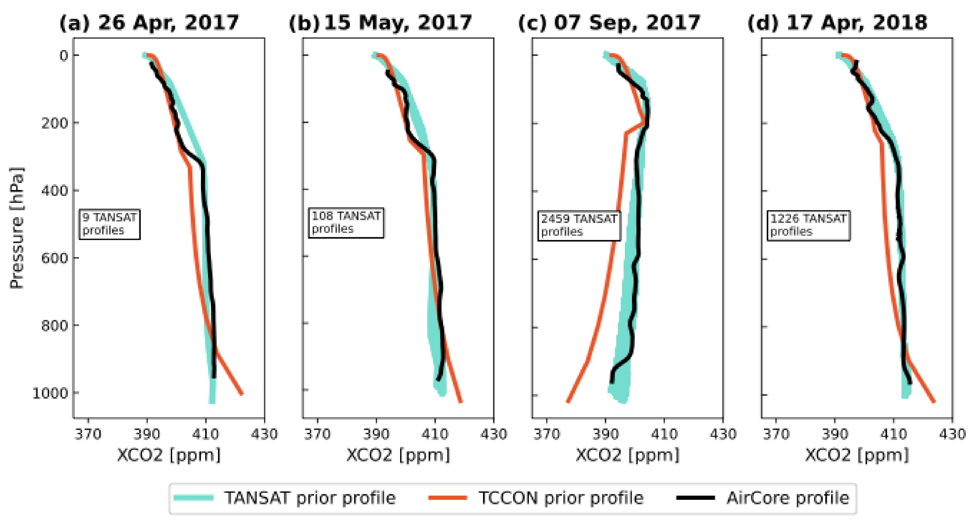
AirCore Comparison in Northern Finland:

In Figure 7, we show the comparisons of TanSat OCFP and Sodankylä TCCON prior CO2 profiles and the CO2 profiles from the local AirCore measurements for four days between 2017 and 2018. The TCCON and AirCore profiles are from the same day but for the TanSat profiles the temporal co-location criterion was ±2 days from the AirCore measurement date and the spatial co-location criteria were ±5° from the Sodankylä TCCON site. Figure 7 shows that the AirCore and TanSat prior profiles are in a good agreement in the lower and the middle atmosphere. The differences occur in the upper atmosphere close to 200–300 hPa and are generally small.

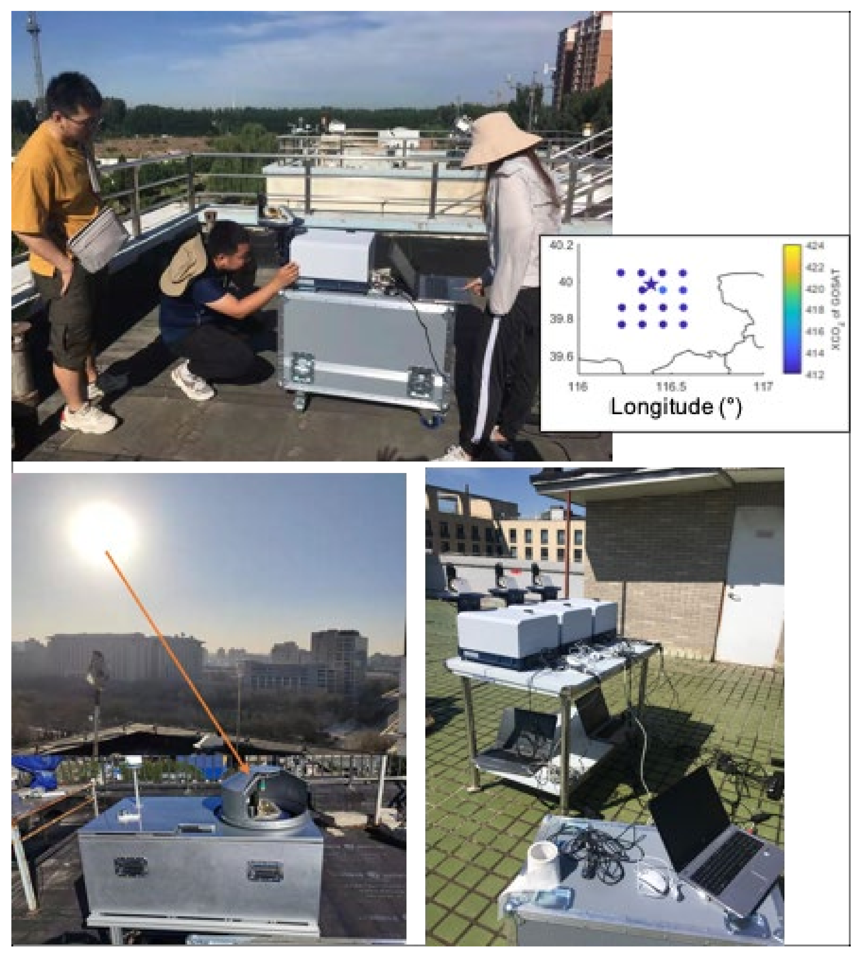
EM27/SUN Observations in Beijing and Comparison with GOSAT Target Mode Observations:

Cities are major contributors of greenhouse gas emissions in the world. Their potential in reducing the emissions is, therefore, also large. In China, the megacity Beijing is a main focus for reducing the emissions of greenhouse gases. Our understanding of regional CO2 and CH4 budget over Beijing mainly comes from target observations of the Greenhouse Gases Observing Satellite (GOSAT). Satellite-borne sensors are sensitive to scattering, the surface albedo model, and the aerosol model, so these satellite data need to be validated and improved in accuracy. A ground-based compact solar-tracking Fourier Transform Spectrometer (Bruker EM27/SUN) has been set up on the roof of the Institute of Atmospheric Physics (IAP) building (39.98°N, 116.39°E) in Beijing. Geographical colocation criteria were used to match GOSAT observations, which are spatially co-located in a radius of 10 km around the ground site. GOSAT overpasses the site at around 15:30 local time, corresponding to high sun elevation, and EM27 observations were selected within ±0.5 h around the satellite overpass time. In Figure 8, the setup of the EM27/SUN instrument is shown on the roof top of the institute. CO2 retrievals from GOSAT for an example overpass over the site are given in the inset in Figure 8, which shows good agreement with the ground-based observation from the EM27. We are now collecting longer time series with the EM27 instruments, which will then allow more detailed comparisons to satellite observations.

AirCore observations in Tibetan Plateau:

Climate change is affecting the Tibetan Plateau strongly with warming temperatures and changes in hydrological cycle. In 2019 and 2020, the Aircore campaign was carried out in Dachaidan (37.3°N, 95.8°E), northeast of the Tibetan Plateau. Fine-scale profiles of CO2 have been retrieved, and Figure 9 shows one example of measured CO2 profiles during the AirCore campaign. The resolution is 0.2–0.4 km in the upper troposphere to lower stratosphere, and in the troposphere, it can reach 0.5–1 km. These in-situ measurement data with the relatively high resolution, especially in the UTLS, is valuable for validating the satellite results in the Tibetan Plateau region.

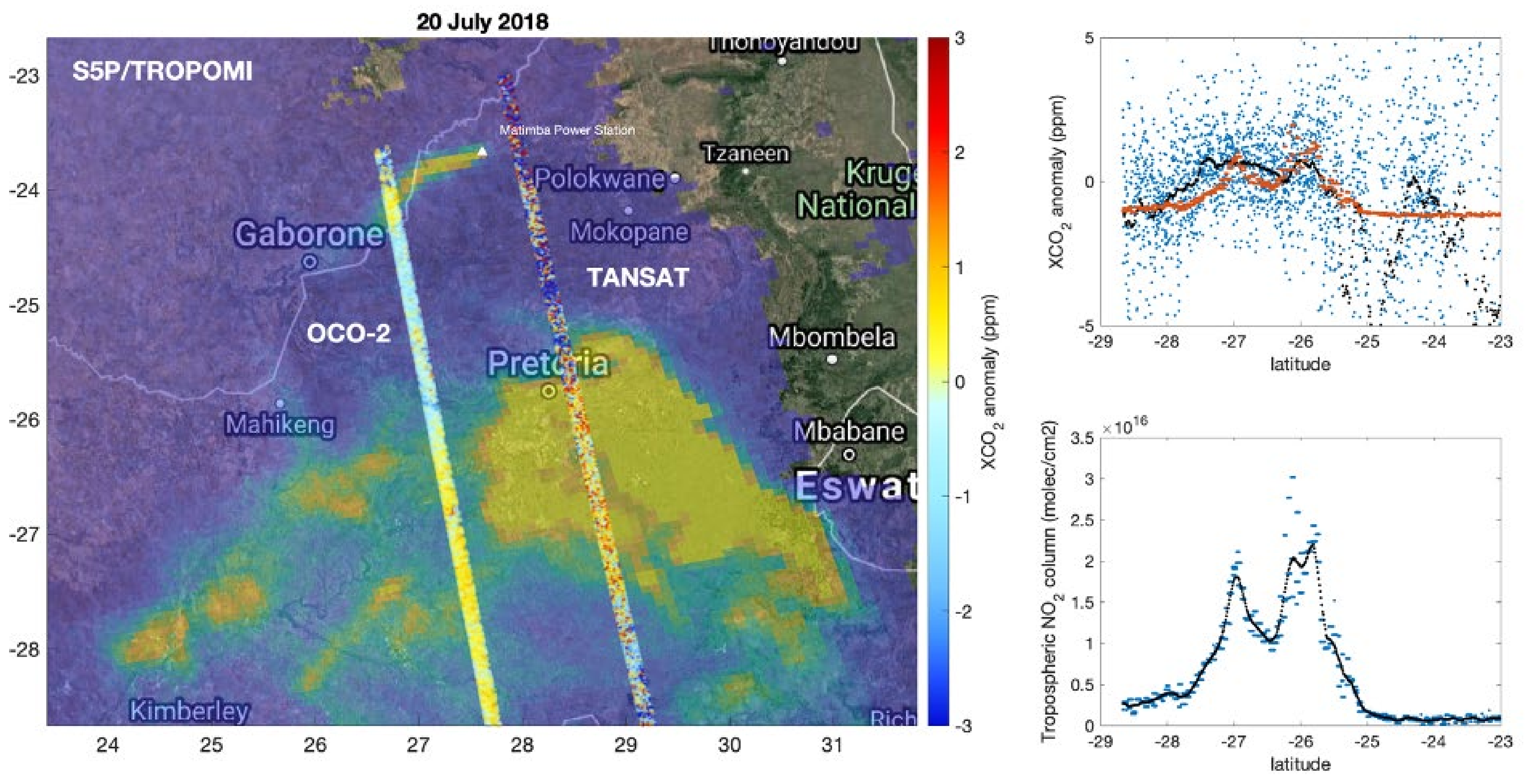
Observing Anthropogenic CO2 Plumes with TanSat:

Since the Paris agreement was adopted in 2015, the role of satellite observations in understanding anthropogenic CO2 emissions has become increasingly important. For example, the European Commission is currently planning a new CO2 monitoring mission CO2M via the Copernicus Programme. The aim is to build a constellation of CO2 measuring satellites with relatively wide swaths (about 250 km). These satellites will also monitor the tropospheric NO2 columns, often recognized as proxy for anthropogenic CO2 [12,13,73]. These observations will, in particular, help the detection of anthropogenic plumes. These plumes can be used to estimate the emissions from individual sources such as power plants and cities.
The main motivation for the current CO2 satellite systems is to reduce the uncertainties of biospheric carbon fluxes on regional scales [74], but they also provided many opportunities to analyse local anthropogenic emissions. The main challenge in observing anthropogenic emissions with satellite instruments, such as the Chinese TanSat and NASA’s OCO-2, is the narrow swath (less than 20 km), which does not allow to detect the plumes in their entirety, but rather the cross-sections. One exception to this is the NASA’s OCO-3 instrument on board the International Space Station, which also takes the measurements in the “Snapshot Area Map” mode [75]. Despite the limitations of the current systems, anthropogenic emissions have been successfully estimated from both power plants and cities. For example, Nassar et al. (2017) [74] provided the very first CO2 emission estimation of power plants with real satellite data using the Gaussian plume model, and Reuter et al. (2019) [76] estimated the emissions from various sources using the cross-sectional flux method [77]. Furthermore, Hakkarainen et al. (2021) [78] proposed a new methodology to derive source-specific NOx-to-CO2 emission ratios using satellite observations.
Figure 10 shows an example of the detection of anthropogenic plumes on 20 July 2018 using TanSat and Sentinel 5P (S5P) satellite data in the Highveld area in South Africa, where several power plants are located. In the background, we illustrate the tropospheric NO2 columns observed by S5P/TROPOMI. The TanSat observations illustrating the cross-section of the CO2 plumes are shown on top. Figure 10 shows the local anomaly derived by subtracting the local median from the observations. The right panels show the cross-sections of the plumes along the TanSat track as a function of latitude. Blue colours indicate the TanSat XCO2 anomalies (top) and TROPOMI tropospheric NO2 columns (bottom). Black colours indicate the running mean. We also converted the observed tropospheric columns to XCO2 via a linear fit (orange colours, top). In addition to TanSat, Figure 10 (left panel) includes the cross-section of the CO2 plumes, as observed by NASA’s OCO-2, during the same day. The OCO-2 observations also show a cross-section of the isolated Matimba power station (CO2 emissions of about 60 kt/d), which was analysed in detail in Hakkarainen et al. (2021) [78].

4.2.2. Summary and Conclusions of Subproject 2

In Subproject 2, TanSat data were evaluated against ground-based and profile measurements as well as data from other satellites. The geographical focus was on the validation sites, high Northern latitudes, and over an example site that includes strong anthropogenic emissions.
Evaluation of TanSat against the ground-based Total Carbon Column Observing Network (TCCON) showed that the mean bias of the TanSat XCO2 varied from –2.9 ppm to 1.4 ppm, and the precision (1-sigma) varied from 0.5 ppm up to 7.0 ppm, depending on the site. The accuracy and precision are comparable to other CO2 satellite missions, considering that the evaluation period was relatively short (15 months) and the evaluation covered only about 400 overpasses.
TanSat XCO2 products were evaluated at high latitudes by comparing to the TCCON and AirCore measurements. Two high-latitude TCCON sites were considered: East Trout Lake in Canada and Sodankylä in Finland. The agreement of TanSat with the TCCON was found to be very good, in terms of small biases (0.07 ppm and –0.21 ppm) and standard deviations (1.2 ppm and 2.5 ppm), and either better than or comparable to the global results. The TanSat prior CO2 profiles were found to agree very well with measured AirCore profiles, with only minor discrepancies in the upper atmosphere. The seasonal coverage of TanSat at high latitudes extended to about 8 months of observations, at a latitude of the Arctic Circle (67°N), and was longer than for OCO-2. The high-latitude biases were found to be seasonally dependent. At both East Trout Lake and Sodankylä, the TanSat biases were negative in the spring and positive in summer and fall. Seasonal variability in the high-latitude bias was somewhat larger than the bias quantified by Jacobs et al. (2020) [79] for OCO-2 but follows partly similar seasonal variability (negative biases in spring, positive during summer). TanSat XCO2 retrieval uncertainty was quantified to be higher over snow than over snow-free landscape, which may indicate that snow conditions contribute to the seasonal bias.
In June 2018, an AirCore campaign was hosted by FMI in Sodankylä. The Chinese Dragon team participated in the campaign and gained experience on the AirCore system that supported launching AirCore flights in the Tibetan Plateau in the following year.
We have also assessed the feasibility of TanSat to observe emission plumes. The narrow swath satellite instruments, such as OCO-2 and TanSat, and are not optimal for detecting anthropogenic emissions from local sources. However, by analysing the observations together with a wide-swath instrument, which detects co-emitted gases such as NO2, the detection of the emission plumes can be improved. This is demonstrated by analysing jointly TanSat and OCO-2 XCO2 anomalies and Sentinel 5 Precursor tropospheric NO2.

5. Main Conclusions

This Dragon-4 project has built a successful collaboration between research groups in UK, Finland, and China with a focus on satellite remote sensing of CO2 validation and modelling using the TanSat and other CO2 missions.
One focus of sub-project 1 was on improving the CO2 retrieval for the TanSat mission benefitting from the availability of two independent retrieval algorithms in the project and from detailed knowledge of the satellite instrument of the CAS group. We could identify an issue with the radiometric calibration, and a suitable correction has been developed and implemented in the European (UoL-FP) and Chinese (IAPCAS) retrieval algorithms which has led to much-improved global TanSat XCO2 datasets, and to a good level of consistency between XCO2, inferred with both retrievals. TanSat XCO2 data has also been evaluated against model calculations of atmospheric CO2 showing good agreement in global distribution of CO2. In the future, we expect that the TanSat XCO2 data will be used for surface flux inversions to complement surface flux estimates available from missions such as OCO-2 and GOSAT.
Evaluation of satellite observations against ground-based reference observations is an important component of Earth observation. It supports improving the retrieval algorithms and characterizes uncertainties related to the observations. In sub-project 2, we have focused on validating TanSat column CO2 observations. Comparisons against TCCON show that the accuracy and precision of TanSat are somewhat worse, but comparable to other CO2 satellite missions. Perhaps surprisingly, comparisons at high latitude sites in Sodankylä, Finland and East Trout Lake, Canada show either better than, or comparable to, the global results. Some seasonal variability in the bias was also observed, which may partly be caused by the higher retrieval uncertainty over snow-covered areas. Overall, seasonally varying biases found at high latitudes and their potential relation to the snow cover are important for further research and retrieval algorithm development.
The retrieval algorithms rely on several assumptions that may affect the retrieval accuracy either in a random or systematic way. One such factor is the assumed a priori profile shape of CO2, typically taken from models. In sub-project 2, we used AirCore profile observations of CO2 in Sodankylä to validate the TanSat a priori profile shapes. The comparisons showed relatively good agreement. Profile observations of CO2 are available only in a few places in the world, limiting such evaluations globally. During the Dragon 4 project, AirCore profile observations were made for the first time in Tibetan Plateau, China.
This project has also contributed to the training and career development of young scientists, and several young scientists from China and Europe are part of the project team, and there has been active exchange of researchers and knowledge, which has directly contributed to the success of the project.
The focus of this project was on the TanSat missions but the findings and outcomes of this project will benefit future missions, such as the Copernicus CO2 Monitoring Mission CO2M or a potential follow-on mission to TanSat. The project also highlights the importance of close collaboration between international research groups in the field of greenhouse gas remote sensing which will be even more important and should be continued to be supported for future missions which aim at monitoring anthropogenic carbon emissions.

Author Contributions

H.B., J.T., H.L., D.Y. have prepared the manuscript; J.H., R.K., L.F., S.P. and E.K. have contributed writing, P.I.P., Y.L., A.J.W. have contributed with reviewing and editing. J.H., R.J.P., A.D.N., N.K. and I.I. have contributed to the methodology development. R.K., T.K. and H.C. have contributed to conducting Sodankylä observations. Z.C., K.C., J.W., L.Y. have contributed to the TanSat retrieval algorithm. All authors have been involved in the research of this project. All authors have read and agreed to the published version of the manuscript.

Funding

This work was supported by the National Key R&D Program of China (Grant No. 2016YFA0600203), the Key Research Program of the Chinese Academy of Sciences (Grant No. ZDRW-ZS-2019-1), the International Partnership Program of the Chinese Academy of Sciences (Grant No. GJHZ201903), the National Natural Science Foundation of China (Grant No. 41905029), ESA Climate Change Initiative CCI+ (GHG theme), Earthnet Data Assessment Pilot (EDAP) project and ESA-MOST Dragon-4 programme (ID 32301). HB, RJP and AW, and PIP and LF are supported by the UK NERC National Centre for Earth Observation (NCEO) (Grant No NE/N018079/1 and NE/R016518/1). The FMI team acknowledges funding from the Academy of Finland (projects 312125, 331829, 337552) and from the ESA DACES, FRM4GHG and SNOWITE. The TanSat L1B data service is provided by IRCSD and CASA (131211KYSB20180002). We also thank the Fengyun Satellite Data Center of the National Satellite Meteorological Center, who provide the TanSat L1B data service. This research used the ALICE High Performance Computing Facility at the University of Leicester. The authors thank the TanSat mission, and the support from everyone involved with the TanSat mission is highly appreciated.

Institutional Review Board Statement

Not applicable.

Informed Consent Statement

Not applicable.

Data Availability Statement

The TanSat IAPCAS v2 XCO2 data product is available from the CASA TanSat data and science service (www.chinageoss.cn/tansat; accessed January 2021). The UoL-FP TanSat data is available from the ESA Climate Change Initiative: http://cci.esa.int/data (accessed October 2020). TCCON data are available from the TCCON Data Archive at https://tccondata.org/ (accessed 28 May 2021). AirCore measurements are available by contacting the authors.

Acknowledgments

For providing the TCCON data we acknowledge Nicholas Deutscher, Justus Notholt, Isamu Morino, Paul Wennberg, David Griffith, Debra Wunch, Laura T. Iraci, Ralf Sussmann, Frank Hase, Dave Pollard, Thorsten Warneke, Yao Té, Kei Shiomi and David Griffith.

Conflicts of Interest

The authors declare no conflict of interest.

References

  1. Dlugokencky, E.; Tans, P. Trends in Atmospheric Carbon Dioxide, National Oceanic and Atmospheric Administration, Earth System Research Laboratory (NOAA/ESRL). Available online: http://www.esrl.noaa.gov/gmd/ccgg/trends/global.html (accessed on 1 March 2021).
  2. Ciais, P.; Tan, J.; Wang, X.; Roedenbeck, C.; Chevallier, F.; Piao, S.-L.; Moriarty, R.; Broquet, G.; Le Quéré, C.; Canadell, J.G.; et al. Five decades of northern land carbon uptake revealed by the interhemispheric CO2 gradient. Nature 2019, 568, 221–225. [Google Scholar] [CrossRef] [Green Version]
  3. Friedlingstein, P.; O’Sullivan, M.; Jones, M.W.; Andrew, R.M.; Hauck, J.; Olsen, A.; Peters, G.P.; Peters, W.; Pongratz, J.; Sitch, S.; et al. Global Carbon Budget 2020. Earth Syst. Sci. Data 2020, 12, 3269–3340. [Google Scholar] [CrossRef]
  4. Bovensmann, H.; Burrows, J.P.; Buchwitz, M.; Frerick, J.; Noël, S.; Rozanov, V.V.; Chance, K.V.; Goede, A.P.H. SCI-AMACHY: Mission objectives and measurement modes. J. Atmos. Sci. 1999, 56, 127–150. [Google Scholar] [CrossRef] [Green Version]
  5. Kuze, A.; Suto, H.; Nakajima, M.; Hamazaki, T. Thermal and near infrared sensor for carbon observation Fourier-transform spectrometer on the Greenhouse Gases Observing Satellite for greenhouse gases monitoring. Appl. Opt. 2009, 48, 6716–6733. [Google Scholar] [CrossRef] [PubMed]
  6. Crisp, D.; Miller, C.E.; De Cola, P.L. NASA Orbiting Carbon Observatory: Measuring the column averaged carbon dioxide mole fraction from space. J. Appl. Remote Sens. 2008, 2, 023508. [Google Scholar] [CrossRef]
  7. Buchwitz, M.; Reuter, M.; Schneising, O.; Hewson, W.; Detmers, R.; Boesch, H.; Hasekamp, O.; Aben, I.; Bovensmann, H.; Burrows, J.P.; et al. Global satellite observations of column-averaged carbon dioxide and methane: The GHG-CCI XCO2 and XCH4 CRDP3 data set. Remote Sens. Environ. 2017, 203, 276–295. [Google Scholar] [CrossRef] [Green Version]
  8. Yang, D.; Liu, Y.; Cai, Z.; Deng, J.; Wang, J.; Chen, X. An advanced carbon dioxide retrieval algorithm for satellite meas-urements and its application to GOSAT observations. Chin. Sci. Bull. 2015, 60, 2063–2066. [Google Scholar] [CrossRef] [Green Version]
  9. O’Dell, C.W.; Eldering, A.; Wennberg, P.O.; Crisp, D.; Gunson, M.R.; Fisher, B.; Frankenberg, C.; Kiel, M.; Lindqvist, H.; Mandrake, L.; et al. Improved retrievals of carbon dioxide from Orbiting Carbon Observatory-2 with the version 8 ACOS algorithm. Atmos. Meas. Tech. 2018, 11, 6539–6576. [Google Scholar] [CrossRef] [Green Version]
  10. Yoshida, Y.; Kikuchi, N.; Morino, I.; Uchino, O.; Oshchepkov, S.; Bril, A.; Saeki, T.; Schutgens, N.; Toon, G.C.; Wunch, D.; et al. Improvement of the retrieval algorithm for GOSAT SWIR XCO2 and XCH4 and their validation using TCCON data. Atmos. Meas. Tech. 2013, 6, 1533–1547. [Google Scholar] [CrossRef]
  11. Palmer, P.I.; Feng, L.; Baker, D.; Chevallier, F.; Bösch, H.; Somkuti, P. Net carbon emissions from African biosphere dominate pan-tropical atmospheric CO2 signal. Nat. Commun. 2019, 10, 1–9. [Google Scholar] [CrossRef] [Green Version]
  12. Hakkarainen, J.; Ialongo, I.; Maksyutov, S.; Crisp, D. Analysis of Four Years of Global XCO2 Anomalies as Seen by Orbiting Carbon Observatory-2. Remote Sens. 2019, 11, 850. [Google Scholar] [CrossRef] [Green Version]
  13. Hakkarainen, J.; Ialongo, I.; Tamminen, J. Direct space-based observations of anthropogenic CO2 emission areas from OCO-2, Geophys. Res. Lett. 2016, 43, 400–406. [Google Scholar] [CrossRef]
  14. Yang, D.; Zhang, H.; Liu, Y.; Chen, B.; Cai, Z.; Lü, D. Monitoring carbon dioxide from space: Retrieval algorithm and flux inversion based on GOSAT data and using CarbonTracker-China. Adv. Atmos. Sci. 2017, 34, 965–976. [Google Scholar] [CrossRef]
  15. Chen, C.; Park, T.; Wang, X.; Piao, S.; Xu, B.; Chaturvedi, R.K.; Fuchs, R.; Brovkin, V.; Ciais, P.; Fensholt, R.; et al. China and India lead in greening of the world through land-use management. Nat. Sustain. 2019, 2, 122–129. [Google Scholar] [CrossRef] [PubMed]
  16. Chen, W.; Zhang, Y.; Yin, Z.; Zheng, Y.; Yan, C.; Yang, Z.; Liu, Y. The TanSat mission: Global CO2 observation and monitoring. In Proceedings of the 63rd IAC (International Astronautical Congress), Naples, Italy, 1–5 October 2012. [Google Scholar]
  17. Ran, Y.; Li, X. TanSat: A new star in global carbon monitoring from China. Sci. Bull. 2019, 64, 284–285. [Google Scholar] [CrossRef] [Green Version]
  18. Lin, C.; Li, C.; Wang, L.; Bi, Y.; Zheng, Y. Preflight spectral calibration of hyperspectral carbon dioxide spectrometer of TanSat. Opt. Precis. Eng. 2017, 25, 2064–2075. (In Chinese) [Google Scholar]
  19. Liu, Y.; Yang, D.; Duan, M.; Cai, Z. Optimization of the instrument configuration for TanSat CO2 spectrometer. Chin. Sci. Bull. 2013, 58, 2787–2789. [Google Scholar] [CrossRef]
  20. Wang, Q.; Yang, Z.D.; Bi, Y.M. Paper Presented at Spectral Parameters and Signal-to-Noise Ratio Requirement for CO2 Hyper Spectral Remote Sensor; SPIE Asia-Pacific Remote Sensing: Beijing, China, 2014. [Google Scholar]
  21. Chen, X.; Yang, D.; Cai, Z.; Liu, Y.; Spurr, R.J.D. Aerosol Retrieval Sensitivity and Error Analysis for the Cloud and Aerosol Polarimetric Imager on Board TanSat: The Effect of Multi-Angle Measurement. Remote Sens. 2017, 9, 183. [Google Scholar] [CrossRef] [Green Version]
  22. Zhang, H.; Zheng, Y.; Li, S.; Lin, C.; Li, C.; Yuan, J.; Li, Y. Geometric correction for TanSat atmospheric carbon dioxide grating spectrometer. Sens. Actuators A Phys. 2019, 293, 62–69. [Google Scholar] [CrossRef]
  23. Yang, D.; Liu, Y.; Cai, Z.; Chen, X.; Yao, L.; Lu, D. First Global Carbon Dioxide Maps Produced from TanSat Measurements. Adv. Atmos. Sci. 2018, 35, 621–623. [Google Scholar] [CrossRef]
  24. Cogan, A.J.; Boesch, H.; Parker, R.J.; Feng, L.; Palmer, P.I.; Blavier, J.-F.L.; Deutscher, N.; Macatangay, R.; Notholt, J.; Roehl, C.; et al. Atmospheric carbon dioxide retrieved from the Greenhouse gases Observing SATellite (GOSAT): Comparison with ground-based TCCON observations and GEOS-Chem model calculations. J. Geophys. Res. Space Phys. 2012, 117. [Google Scholar] [CrossRef] [Green Version]
  25. Somkuti, P.; Bösch, H.; Parker, R. The Significance of Fast Radiative Transfer for Hyperspectral SWIR XCO2 Retrievals. Atmosphere 2020, 11, 1219. [Google Scholar] [CrossRef]
  26. Feng, L.; Palmer, P.I.; Bösch, H.; Parker, R.J.; Webb, A.J.; Correia, C.S.C.; Deutscher, N.M.; Domingues, L.G.; Feist, D.G.; Gatti, L.V.; et al. Consistent regional fluxes of CH4 and CO2 inferred from GOSAT proxy XCH4: XCO2 retrievals, 2010–2014. Atmos. Chem. Phys. 2017, 17, 4781–4797. [Google Scholar] [CrossRef] [Green Version]
  27. Kivi, R.; Heikkinen, P. Fourier transform spectrometer measurements of column CO2 at Sodankylä, Finland. Geosci. Instrum. Methods Data Syst. 2016, 5, 271–279. [Google Scholar] [CrossRef] [Green Version]
  28. Inoue, M.; Morino, I.; Uchino, O.; Nakatsuru, T.; Yoshida, Y.; Yokota, T.; Wunch, D.; Wennberg, P.O.; Roehl, C.M.; Griffith, D.W.T.; et al. Bias corrections of GOSAT SWIR XCO2 and XCH4 with TCCON data and their evaluation using aircraft measurement data. Atmos. Meas. Tech. 2016, 9, 3491–3512. [Google Scholar] [CrossRef] [Green Version]
  29. Wunch, D.; Wennberg, P.O.; Osterman, G.; Fisher, B.; Naylor, B.; Roehl, C.M.; O’Dell, C.; Mandrake, L.; Viatte, C.; Kiel, M.; et al. Comparisons of the Orbiting Carbon Observatory-2 (OCO-2) XCO2 measurements with TCCON. Atmos. Meas. Tech. 2017, 10, 2209–2238. [Google Scholar] [CrossRef] [Green Version]
  30. Borsdorff, T.; de Brugh, A.J.; Schneider, A.; Lorente, A.; Birk, M.; Wagner, G.; Kivi, R.; Hase, F.; Feist, D.G.; Sussmann, R.; et al. Improving the TROPOMI CO data product: Update of the spectroscopic database and destriping of single orbits. Atmos. Meas. Tech. 2019, 12, 5443–5455. [Google Scholar] [CrossRef] [Green Version]
  31. Lorente, A.; Borsdorff, T.; Butz, A.; Hasekamp, O.; De Brugh, J.A.; Schneider, A.; Wu, L.; Hase, F.; Kivi, R.; Wunch, D.; et al. Methane retrieved from TROPOMI: Improvement of the data product and validation of the first 2 years of measurements. Atmos. Meas. Tech. 2021, 14, 665–684. [Google Scholar] [CrossRef]
  32. Sha, M.K.; Langerock, B.; Blavier, J.-F.L.; Blumenstock, T.; Borsdorff, T.; Buschmann, M.; Dehn, A.; De Mazière, M.; Deutscher, N.M.; Feist, D.G.; et al. Validation of Methane and Carbon Monoxide from Sentinel-5 Precursor using TCCON and NDACC-IRWG stations. Atmos. Meas. Tech. Discuss. 2021. in review. [Google Scholar] [CrossRef]
  33. Karion, A.; Sweeney, C.; Tans, P.; Newberger, T. AirCore: An Innovative Atmospheric Sampling System. J. Atmos. Ocean. Technol. 2010, 27, 1839–1853. [Google Scholar] [CrossRef]
  34. Tukiainen, S.; Railo, J.; Laine, M.; Hakkarainen, J.; Kivi, R.; Heikkinen, P.; Chen, H.; Tamminen, J. Retrieval of atmospheric CH4 profiles from Fourier transform infrared data using dimension reduction and MCMC. J. Geophys. Res. Atmos. 2016, 121, 312. [Google Scholar] [CrossRef] [Green Version]
  35. Zhou, M.; Langerock, B.; Sha, M.K.; Kumps, N.; Hermans, C.; Petri, C.; Warneke, T.; Chen, H.; Metzger, J.-M.; Kivi, R.; et al. Retrieval of atmospheric CH4 vertical information from ground-based FTS near-infrared spectra. Atmos. Meas. Tech. 2019, 12, 6125–6141. [Google Scholar] [CrossRef]
  36. Sha, M.K.; De Mazière, M.; Notholt, J.; Blumenstock, T.; Chen, H.; Dehn, A.; Griffith, D.W.T.; Hase, F.; Heikkinen, P.; Hermans, C.; et al. Intercomparison of low- and high-resolution infrared spectrometers for ground-based solar remote sensing measurements of total column concentrations of CO2, CH4, and CO. Atmos. Meas. Tech. 2020, 13, 4791–4839. [Google Scholar] [CrossRef]
  37. Tu, Q.; Hase, F.; Blumenstock, T.; Kivi, R.; Heikkinen, P.; Sha, M.K.; Raffalski, U.; Landgraf, J.; Lorente, A.; Borsdorff, T.; et al. Intercomparison of atmospheric CO2 and CH4 abundances on regional scales in boreal areas using Copernicus Atmosphere Monitoring Service (CAMS) analysis, COllaborative Carbon Column Observing Network (COCCON) spectrometers, and Sentinel-5 Precursor satellite observations. Atmos. Meas. Tech. 2020, 13, 4751–4771. [Google Scholar] [CrossRef]
  38. Schneider, M.; Ertl, B.; Diekmann, C.J.; Khosrawi, F.; Röhling, A.N.; Hase, F.; Dubravica, D.; García, O.E.; Sepúlveda, E.; Borsdorff, T.; et al. Synergetic use of IASI and TROPOMI space borne sensors for generating a tropospheric methane profile product. Atmos. Meas. Tech. Discuss. 2021. in review. [Google Scholar] [CrossRef]
  39. Toon, G.C. Solar Line List for GGG2014, TCCON Data Archive. Hosted by the Carbon Dioxide Information Analysis Center, Oak; Ridge National Laboratory: Oak Ridge, TN, USA, 2017. [Google Scholar] [CrossRef]
  40. Meftah, M.; Damé, L.; Bolsée, D.; Hauchecorne, A.; Pereira, N.; Sluse, D.; Cessateur, G.; Irbah, A.; Bureau, J.; Weber, M.; et al. SOLAR-ISS: A new reference spectrum based on SOLAR/SOLSPEC observations. Astron. Astrophys. 2018, 611, A1. [Google Scholar] [CrossRef]
  41. Yang, D.; Boesch, H.; Liu, Y.; Somkuti, P.; Cai, Z.; Chen, X.; Di Noia, A.; Lin, C.; Lu, N.; Lyu, D.; et al. Toward High Precision XCO 2 Retrievals from TanSat Observations: Retrieval Improvement and Validation Against TCCON Measurements. J. Geophys. Res. Atmos. 2020, 125, 032794. [Google Scholar] [CrossRef]
  42. Yang, D.; Liu, Y.; Boesch, H.; Yao, L.; Di Noia, A.; Cai, Z.; Lu, N.; Lyu, D.; Wang, M.; Wang, J.; et al. A New TanSat XCO2 Global Product towards Climate Studies. Adv. Atmos. Sci. 2021, 38, 8–11. [Google Scholar] [CrossRef]
  43. Liu, Y.; Wang, J.; Yao, L.; Chen, X.; Cai, Z.; Yang, D.; Yin, Z.; Gu, S.; Tian, L.; Lu, N.; et al. The TanSat mission: Preliminary global observations. Sci. Bull. 2018, 63, 1200–1207. [Google Scholar] [CrossRef] [Green Version]
  44. Aben, I.; Hasekamp, O.; Hartmann, W. Uncertainties in the space-based measurements of CO2 columns due to scattering in the Earth’s atmosphere. J. Quant. Spectrosc. Radiat. Transf. 2007, 104, 3. [Google Scholar] [CrossRef]
  45. Boesch, H.; Liu, Y.; Palmer, P.I.; Tamminen, J.; Anand, J.S.; Cai, Z.; Che, K.; Chen, H.; Chen, X.; Feng, L.; et al. Monitoring Greenhouses Gases over China Using Space-Based Observations. J. Geod. Geoinf. Sci. 2020, 3, 14–24. [Google Scholar]
  46. Connor, B.J.; Boesch, H.; Toon, G.; Sen, B.; Miller, C.; Crisp, D. Orbiting Carbon Observatory: Inverse method and prospective error analysis. J. Geophys. Res. Space Phys. 2008, 113, D05305. [Google Scholar] [CrossRef]
  47. Wang, J.; Feng, L.; Palmer, P.I.; Liu, Y.; Fang, S.; Bösch, H.; O’Dell, C.W.; Tang, X.; Yang, D.; Liu, L.; et al. Large Chinese land carbon sink estimated from atmospheric carbon dioxide data. Nat. Cell Biol. 2020, 586, 720–723. [Google Scholar] [CrossRef]
  48. Wunch, D.; Toon, G.C.; Blavier, J.-F.L.; Washenfelder, R.; Notholt, J.; Connor, B.J.; Griffith, D.W.T.; Sherlock, V.; Wennberg, P.O. The Total Carbon Column Observing Network. Philos. Trans. R. Soc. A Math. Phys. Eng. Sci. 2011, 369, 2087–2112. [Google Scholar] [CrossRef] [Green Version]
  49. Lindqvist, H.; Odell, C.W.; Basu, S.; Boesch, E.H.; Chevallier, F.; Deutscher, N.M.; Feng, L.; Fisher, B.M.; Hase, F.; Inoue, M.; et al. Does GOSAT capture the true seasonal cycle of carbon dioxide? Atmos. Chem. Phys. Discuss. 2015, 15, 13023–13040. [Google Scholar] [CrossRef] [Green Version]
  50. Kivimäki, E.; Lindqvist, H.; Hakkarainen, J.; Laine, M.; Sussmann, R.; Tsuruta, A.; Detmers, R.; Deutscher, N.M.; Dlugokencky, E.J.; Hase, F.; et al. Evaluation and Analysis of the Seasonal Cycle and Variability of the Trend from GOSAT Methane Retrievals. Remote Sens. 2019, 11, 882. [Google Scholar] [CrossRef] [Green Version]
  51. Deutscher, N.M.; Notholt, J.; Messerschmidt, J.; Weinzierl, C.; Warneke, T.; Petri, C.; Grupe, P. TCCON Data from Bialystok (PL), Release GGG2014.R2 (Version R2), TCCON Data Archive, Hosted by CaltechDATA. 2019. Available online: https://doi.org/10.14291/TCCON.GGG2014.BIALYSTOK01.R2 (accessed on 28 May 2021).
  52. Notholt, J.; Petri, C.; Warneke, T.; Deutscher, N.M.; Palm, M.; Buschmann, M.; Weinzierl, C.; Macatangay, R.C.; Grupe, P. TCCON Data from Bremen (DE), Release GGG2014.R1 (Version R1), TCCON Data Archive, Hosted by CaltechDATA. 2019. Available online: https://doi.org/10.14291/TCCON.GGG2014.BREMEN01.R1 (accessed on 28 May 2021).
  53. Morino, I.; Velazco, V.A.; Akihiro, H.; Osamu, U.; Griffith, D.W.T. TCCON Data from Burgos, Ilocos Norte (PH), Release GGG2014.R0 (Version GGG2014.R0), TCCON Data Archive, Hosted by CaltechDATA. 2018. Available online: https://doi.org/10.14291/tccon.ggg2014.burgos01.R0 (accessed on 28 May 2021).
  54. Wennberg, P.O.; Wunch, D.; Roehl, C.; Blavier, J.-F.; Toon, G.C.; Allen, N. TCCON data from Caltech (US), Release GGG2014R1 (Version GGG2014.R1), TCCON Data Archive, Hosted by CaltechDATA. 2015. Available online: https://doi.org/10.14291/tccon.ggg2014.pasadena01.R1/1182415 (accessed on 28 May 2021).
  55. Griffith, D.W.; Deutscher, N.M.; Velazco, V.A.; Wennberg, P.O.; Yavin, Y.; Aleks, G.K.; Washenfelder, R.; Toon, G.C.; Blavier, J.-F.; Murphy, C.; et al. TCCON Data from Darwin (AU), Release GGG2014R0 (Version GGG2014.R0), TCCON Data Archive, Hosted by CaltechDATA. 2014. Available online: https://doi.org/10.14291/tccon.ggg2014.darwin01.R0/1149290 (accessed on 28 May 2021).
  56. Wunch, D.; Mendonca, J.; Colebatch, O.; Allen, N.; Blavier, J.-F.L.; Roche, S.; Hedelius, J.K.; Neufeld, G.; Springett, S.; Worthy, D.E.J.; et al. TCCON Data from East Trout Lake (CA), Release GGG2014R1 (Version R1), TCCON Data Archive, Hosted by CaltechDATA. 2018. Available online: https://doi.org/10.14291/tccon.ggg2014.easttroutlake01.R1 (accessed on 28 May 2021).
  57. Iraci, L.T.; Podolske, J.; Hillyard, P.W.; Roehl, C.; Wennberg, P.O.; Blavier, J.-F.; Allen, N.; Wunch, D.; Osterman, G.B.; Albertson, R. TCCON Data from Edwards (US), Release GGG2014R1 (Version GGG2014.R1), TCCON Data Archive, Hosted by CaltechDATA. 2016. Available online: https://doi.org/10.14291/tccon.ggg2014.edwards01.R1/1255068 (accessed on 28 May 2021).
  58. Sussmann, R.; Rettinger, M. TCCON Data from Garmisch (DE), Release GGG2014.R2 (Version R2), TCCON Data Archive, Hosted by CaltechDATA. 2018. Available online: https://doi.org/10.14291/TCCON.GGG2014.GARMISCH01.R2 (accessed on 28 May 2021).
  59. Wennberg, P.O.; Roehl, C.M.; Blavier, J.-F.; Wunch, D.; Allen, N.T. TCCON data from Jet Propulsion Laboratory (US), 2011, Release GGG2014.R1 (Version GGG2014.R1), TCCON Data Archive, Hosted by CaltechDATA. 2016a. Available online: https://doi.org/10.14291/TCCON.GGG2014.JPL02.R1/1330096 (accessed on 28 May 2021).
  60. Hase, F.; Blumenstock, T.; Dohe, S.; Gross, J.; Kiel, M. TCCON Data from Karlsruhe (DE), Release GGG2014R1, TCCON Data Archive, Hosted by CaltechDATA. 2014. Available online: https://doi.org/10.14291/tccon.ggg2014.karlsruhe01.R1/1182416 (accessed on 28 May 2021).
  61. Wennberg, P.O.; Wunch, D.; Roehl, C.; Blavier, J.F.; Toon, G.C.; Allen, N.; Dowell, P.; Teske, K.; Martin, C.; Martin, J. TCCON Data from Jet Propulsion Laboratory (US), 2011, Release GGG2014.R1 (Version GGG2014.R1), TCCON Data Archive, Hosted by CaltechDATA. 2016b. Available online: https://doi.org/10.14291/TCCON.GGG2014.LAMONT01.R1/1255070 (accessed on 28 May 2021).
  62. Sherlock, V.; Connor, B.; Robinson, J.; Shiona, H.; Smale, D.; Pollard, D.F. TCCON data from Lauder (NZ), 125HR, Release GGG2014.R0 (Version GGG2014.R0), TCCON Data Archive, Hosted by CaltechDATA. 2014. Available online: https://doi.org/10.14291/TCCON.GGG2014.LAUDER02.R0/1149298 (accessed on 28 May 2021).
  63. Pollard, D.F.; Robinson, J.; Shiona, H. TCCON Data from Lauder (NZ), Release GGG2014.R0 (Version GGG2014.R0), TCCON Data Archive, Hosted by CaltechDATA. 2019. Available online: https://doi.org/10.14291/TCCON.GGG2014.LAUDER03.R0 (accessed on 28 May 2021).
  64. Warneke, T.; Messerschmidt, J.; Notholt, J.; Weinzierl, C.; Deutscher, N.M.; Petri, C.; Grupe, P. TCCON data from Orléans (FR), Release GGG2014.R1 (Version R1), TCCON Data Archive, Hosted by CaltechDATA. 2019. Available online: https://doi.org/10.14291/TCCON.GGG2014.ORLEANS01.R1 (accessed on 28 May 2021).
  65. Te, Y.; Jeseck, P.; Janssen, C. TCCON Data from Paris (FR), Release GGG2014R0 (Version GGG2014.R0), TCCON Data Archive, Hosted by CaltechDATA. 2014. Available online: https://doi.org/10.14291/tccon.ggg2014.paris01.R0/1149279 (accessed on 28 May 2021).
  66. Wennberg, P.O.; Roehl, C.M.; Wunch, D.; Toon, G.C.; Blavier, J.-F.; Washenfelder, R.; Keppel-Aleks, G.; Allen, N.T.; Ayers, J. TCCON Data from Park Falls (US), Release GGG2014.R1 (Version GGG2014.R1), TCCON Data Archive, Hosted by CaltechDATA. 2017. Available online: https://doi.org/10.14291/TCCON.GGG2014.PARKFALLS01.R1 (accessed on 28 May 2021).
  67. Morino, I.; Yokozeki, N.; Matzuzaki, T.; Horikawa, M. TCCON Data from Rikubetsu (JP), Release GGG2014R2, TCCON Data Drchive, Hosted by CaltechDATA. 2018. Available online: https://doi.org/10.14291/tccon.ggg2014.rikubetsu01.R2 (accessed on 28 May 2021).
  68. Kawakami, S.; Ohyama, H.; Arai, K.; Okumura, H.; Taura, C.; Fukamachi, T.; Sakashita, M. TCCON Data from Saga (JP), Release GGG2014R0 (Version GGG2014.R0), TCCON Data Archive, Hosted by CaltechDATA. 2014. Available online: https://doi.org/10.14291/tccon.ggg2014.saga01.R0/1149283 (accessed on 28 May 2021).
  69. Kivi, R.; Heikkinen, P.; Kyrö, E. TCCON Data from Sodankyla (FI), Release GGG2014R0 (Version GGG2014.R0), TCCON Data Archive, Hosted by CaltechDATA. 2014. Available online: https://doi.org/10.14291/tccon.ggg2014.sodankyla01.R0/1149280 (accessed on 28 May 2021).
  70. Morino, I.; Matsuzaki, T.; Horikawa, M. TCCON Data from Tsukuba (JP), 125HR, Release GGG2014.R2 (Version R2), TCCON Data Archive, Hosted by CaltechDATA. 2018. Available online: https://doi.org/10.14291/TCCON.GGG2014.TSUKUBA02.R2 (accessed on 28 May 2021).
  71. Griffith, D.W.; Velazco, V.A.; Deutscher, N.M.; Murphy, C.; Jones, N.; Wilson, S.; Macatangay, R.; Kettlewell, G.; Buchholz, R.R.; Riggenbach, M. TCCON Data from Wollongong (AU), Release GGG2014R0 (Version GGG2014.R0), TCCON Data Archive, Hosted by CaltechDATA. 2014. Available online: https://doi.org/10.14291/tccon.ggg2014.wollongong01.R0/1149291 (accessed on 28 May 2021).
  72. Sussmann, R.; Rettinger, M. TCCON Data from Zugspitze (DE), Release GGG2014R1 (Version R1), TCCON Data Archive, Hosted by CaltechDATA. 2018. Available online: https://doi.org/10.14291/tccon.ggg2014.zugspitze01.R1 (accessed on 28 May 2021).
  73. Reuter, M.; Buchwitz, M.; Hilboll, A.; Richter, A.; Schneising, O.; Hilker, M.; Heymann, J.; Bovensmann, H.; Burrows, J.P. Decreasing emissions of NOx relative to CO2 in East Asia inferred from satellite observations. Nat. Geosci. 2014, 7, 792–795. [Google Scholar] [CrossRef]
  74. Nassar, R.; Hill, T.G.; McLinden, C.A.; Wunch, D.; Jones, D.B.A.; Crisp, D. Quantifying CO2 Emissions from Individual Power Plants from Space. Geophys. Res. Lett. 2017, 44. [Google Scholar] [CrossRef] [Green Version]
  75. Kiel, M.; Eldering, A.; Roten, D.D.; Lin, J.C.; Feng, S.; Lei, R.; Lauvaux, T.; Oda, T.; Roehl, C.M.; Blavier, J.-F.; et al. Urban-focused satellite CO2 observations from the Orbiting Carbon Observatory-3: A first look at the Los Angeles megacity. Remote Sens. Environ. 2021, 258, 112314. [Google Scholar] [CrossRef]
  76. Reuter, M.; Buchwitz, M.; Schneising, O.; Krautwurst, S.; O’Dell, C.W.; Richter, A.; Bovensmann, H.; Burrows, J.P. Towards monitoring localized CO2 emissions from space: Co-located regional CO2 and NO2 enhancements observed by the OCO-2 and S5P satellites. Atmos. Chem. Phys. Discuss. 2019, 19, 9371–9383. [Google Scholar] [CrossRef] [Green Version]
  77. Varon, D.J.; Jacob, D.J.; McKeever, J.; Jervis, D.; Durak, B.O.A.; Xia, Y.; Huang, Y. Quantifying methane point sources from fine-scale satellite observations of atmospheric methane plumes. Atmos. Meas. Tech. 2018, 11, 5673–5686. [Google Scholar] [CrossRef] [Green Version]
  78. Hakkarainen, J.; Szeląg, M.E.; Ialongo, I.; Retscher, C.; Oda, T.; Crisp, D. Analyzing nitrogen oxides to carbon dioxide emission ratios from space: A case study of Matimba Power Station in South Africa. Atmos. Environ. X 2021, 10, 100110. [Google Scholar] [CrossRef]
  79. Jacobs, N.; Simpson, W.R.; Wunch, D.; O’Dell, C.W.; Osterman, G.B.; Hase, F.; Blumenstock, T.; Tu, Q.; Frey, M.; Dubey, M.K.; et al. Quality controls, bias, and seasonality of CO2 columns in the boreal forest with Orbiting Carbon Observatory-2, Total Carbon Column Observing Network, and EM27/SUN measurements. Atmos. Meas. Tech. 2020, 13, 5033–5063. [Google Scholar] [CrossRef]
Figure 1. Seasonal maps of the IAPCAS TanSat v2 dataset.
Remotesensing 13 02700 g001
Figure 2. Intercomparison between TanSat XCO2 retrieval from the IAPCAS (v2) retrieval and the UoL-FP retrieval for cloud-free, quality-filtered soundings for overpasses over TCCON sites. The colour coding gives the number of data point per 0.15 ppm bin.
Remotesensing 13 02700 g002
Figure 3. Comparison of the TanSat XCO2 v2 dataset from IAPCAS (a) with the GEOS-Chem model (b). The GEOS-Chem model driven by surface fluxes that have been optimised with surface in-situ data. GEOS-Chem model output is sampled according to the location of cloud-free, quality-filtered TanSat retrievals. The colour scale gives XCO2 in ppm.
Remotesensing 13 02700 g003
Figure 4. Net CO2 fluxes (natural + anthropogenic) over China, averaged for 2010 to 2016 after assimilating additional in-situ sites operated by CMA. Details on the used data and the surface flux inversion can be found in [47].
Remotesensing 13 02700 g004
Figure 5. Evaluation of TanSat OCFP against the TCCON at East Trout Lake, Canada (ac), Saga, Japan (df), and Lauder, New Zealand (gi). Left columns present 1:1 comparison of the daily median XCO2 and a linear fit (dashed line); middle columns show XCO2 time series of the TCCON and TanSat (symbols) and an optimised seasonal cycle fit (solid lines); right columns present the time series of the bias determined as TanSat XCO2—TCCON XCO2. The grey areas depict the 1σ deviation from the mean bias.
Remotesensing 13 02700 g005
Figure 6. Comparison of XCO2 retrievals at Sodankylä, in Northern Finland. Ground-based FTS retrievals from the TCCON are presented with gray symbols. Two retrieval products for TanSat (OCFP with orange and IAPCAS with purple) are shown together with OCO-2 B10 XCO2 (blue symbols). Satellite data are aggregated as daily medians.
Remotesensing 13 02700 g006
Figure 7. TanSat prior CO2 profiles (turquoise), TCCON prior CO2 profiles (red) and measured CO2 profiles from the AirCore (black) for (a) 26 April 2017; (b) 15 May 2017; (c) 7 September 2017; (d) 17 April 2018. TanSat profiles are collected from retrievals within ±2 days from the AirCore date with the spatial co-location criteria of ±5° from the Sodankylä TCCON site. The number of co-located TanSat profiles is indicated in each subplot.
Remotesensing 13 02700 g007
Figure 8. EM27/Sun observations in Beijing. Top right, calibration of the EM27/SUN with 125HR in Xianghe, Hebei. Bottom left: Portable automated enclosure for EM27/SUN. Bottom right: Cross validation of multiple EM27/SUN at Institute of Atmospheric Physics (IAP) at urban Beijing. Top right: Comparison of GOSAT and EM27 XCO2 observation. EM27 site is indicated by pentacle.
Remotesensing 13 02700 g008
Figure 9. Top right: The launch of AirCore on Tibetan Plateau in 2020. Example of vertical CO2 profile observations in Dachaidan, Tibetan Plateau during the 2019–2020 AirCore campaign. Top left: Bottom: Recovery of Aerosol sounding and AirCore on Tibetan Plateau in 2020.
Remotesensing 13 02700 g009
Figure 10. An example of the detection of anthropogenic plumes using TanSat, OCO-2 and Sentinel 5P satellites in Highveld area in South Africa, where several power plants are located. In the subpanels, we illustrate the cross-sections of the plumes along the TanSat track as a function of latitude. Blue colours indicate the TanSat XCO2 anomalies (top) and TROPOMI tropospheric NO2 columns (bottom). Black colours indicate the running mean. We also converted the observed tropospheric NO2 columns to XCO2 via linear fit (orange colours, top).
Remotesensing 13 02700 g010
Table 1. Specifications of key characteristics of the Atmospheric Carbon Dioxide Grating Spectrometer (ACGS).
O2-ACO2 WeakCO2 Strong
Spectral Range (nm)758–7781594–16242042–2082
Spectral Resolution (nm)0.039–0.0420.123–0.1280.16–0.17
Signal to Noise Ratio (SNR) 1[email protected] W m−2 sr−1 nm−1 [email protected] W m−2 sr−1 nm−1[email protected] W m−2 sr−1 nm−1
Spatial Resolution 2 km × 2 km
Swath 18 km
1 Mean SNR through all pixels.
Table 2. Overview over project teaming.
NameInstitutionRoleSub-Project
Hartmut BoeschUniversity of LeicesterEuropean PI for Sub-Project 11
Dongxu YangInstitute of Atmospheric Physics, CASChinese PI for Sub-Project 11
Johnanna TamminenFinnish Meteorological InstituteEuropean PI for Sub-Project 22
Yi LiuInstitute of Atmospheric Physics, CASChinese PI for Sub-Project 22
Paul PalmerUniversity of EdinburghEuropean Team Member1
Zhaonan CaiInstitute of Atmospheric Physics, CASChinese Team Member2
Ke CheInstitute of Atmospheric Physics, CASEuropean Young Scientist2
Huilin ChenUniversity of Groningen,Project Partner2
Antonio Di NoiaUniversity of LeicesterEuropean Team Member1
Liang FengUniversity of EdinburghEuropean Team Member1
Janne HakkarainenFinnish Meteorological InstituteEuropean Team Member2
Iolanda IalongoFinnish Meteorological InstituteEuropean Team Member2
Nikoleta KalaitziUniversity of LeicesterEuropean Young Scientist1
Tomi KarppinenFinnish Meteorological InstituteEuropean Young Scientist2
Rigel KiviFinnish Meteorological InstituteEuropean Team Member2
Ella KivimäkiFinnish Meteorological InstituteEuropean Young Scientist2
Hannakaisa LindqvistFinnish Meteorological InstituteEuropean Team Member2
Robert ParkerUniversity of LeicesterEuropean Team Member1
Simon PrevalUniversity of LeicesterEuropean Team Member1
Jing WangInstitute of Atmospheric Physics, CASChinese Young Scientist1
Alex WebbUniversity of LeicesterEuropean Team Member1
Lu YaoInstitute of Atmospheric Physics, CASChinese Team Member1
Table 3. EO and other datasets utilised in this project.
NameCoverageComment
Chinese EO DataTansat L1/L2Global
ESA, Explorers & Sentinels dataSentinel 5P L2Global
ESA Third Party MissionsGOSAT L1/L2Global
Other missionsOCO-2Global
Other DataTCCONGlobal~30 Sites distributed globally
AirCore
EM27/SUN
Finland and
Tibetan Plateau, China
Beijing, China
In-situ CO2China
Publisher’s Note: MDPI stays neutral with regard to jurisdictional claims in published maps and institutional affiliations.

