Novel Machine Learning Method Integrating Ensemble Learning and Deep Learning for Mapping Debris-Covered Glaciers

Abstract

Glaciers in High Mountain Asia (HMA) have a significant impact on human activity. Thus, a detailed and up-to-date inventory of glaciers is crucial, along with monitoring them regularly. The identification of debris-covered glaciers is a fundamental and yet challenging component of research into glacier change and water resources, but it is limited by spectral similarities with surrounding bedrock, snow-affected areas, and mountain-shadowed areas, along with issues related to manual discrimination. Therefore, to use fewer human, material, and financial resources, it is necessary to develop better methods to determine the boundaries of debris-covered glaciers. This study focused on debris-covered glacier mapping using a combination of related technologies such as random forest (RF) and convolutional neural network (CNN) models. The models were tested on Landsat 8 Operational Land Imager (OLI)/Thermal Infrared Sensor (TIRS) data and the Advanced Spaceborne Thermal Emission and Reflection Radiometer Global Digital Elevation Model (ASTER GDEM), selecting Eastern Pamir and Nyainqentanglha as typical glacier areas on the Tibetan Plateau to construct a glacier classification system. The performances of different classifiers were compared, the different classifier construction strategies were optimized, and multiple single-classifier outputs were obtained with slight differences. Using the relationship between the surface area covered by debris and the machine learning model parameters, it was found that the debris coverage directly determined the performance of the machine learning model and mitigated the issues affecting the detection of active and inactive debris-covered glaciers. Various classification models were integrated to ascertain the best model for the classification of glaciers.

1. Introduction

Glacier changes have significant effects on the local climate, ecological environment, water resources, and sea-level rise [1,2,3]. From the perspective of global warming, the average temperature of High Mountain Asia (HMA) [4,5]—a region that has the largest number of glaciers (95,500) and ice reserves (7.02 ± 1.82 × 10³ km³) outside of the polar regions [6]—has also risen [7,8]. This has put the Qinghai–Tibet Plateau in a state of negative energy balance on the surface, causing most glaciers to retreat [9,10]. Most glacier inventory datasets include glacier boundaries, which are important for studying the spatial distribution of global or regional glaciers. Further, glacier classification is a crucial step in glacier inventory [11]. The parameters from the glacier inventory help inform fields related to the national economy and people’s livelihoods, and they include information regarding water resource utilization, climate change research, and ecological environment construction [12,13]. Through the study of glacier changes, it is possible to ascertain glacier dynamics [14], which has significant research value for understanding past glacial behavior and predicting future climate, environmental, and water resource changes [15].

Mountain glaciers are located in high-altitude remote mountainous areas, which have complex terrains [16,17,18,19]. Since these glaciers are of various types, traditional ground survey methods cannot adequately track large-scale, periodic, systematic, and comprehensive glacier changes. A technique to effectively measure and monitor mountain glaciers is crucial at this stage [16,17,18]. However, in high mountain areas, which experience frequent cloud activity and have a large amount of debris coverage, automatic and semi-automatic glacier mapping based on remote sensing images is challenging [1,11,20], and short-term studies such as these do not necessarily show stable changes over time. Debris-covered glaciers are a special type of glacier [21,22]. The surfaces of mountain glaciers are frequently covered in supraglacial debris, whose spectral characteristics are similar to those of rocks and soil at the foot of the mountain [21,23], making them hard to distinguish from rock glaciers and periglacial areas [24]. Particularly in the Tibetan Plateau, owing to the influence of the monsoon climate, frequent cloud activity occurs during the glacier melting period. This, in combination with topographical cloud influences [25], makes it very difficult to obtain high-quality cloud-free images. Seasonal snow cover and debris also increase the difficulty and uncertainty of glacier boundary identification [25,26]. These uncertain factors cause significant interference in research on glacier distribution, water storage, glacier changes, hydrological modeling, and information extraction on the local and regional scales, which is the focus [27] of current research on glaciers [21].

By combining machine learning methods to analyze and extract features based on the different dimensions of the glacier remote sensing images in each pixel, a rapid automatic classification of glaciers can be achieved, clearly reflecting the various glacier types [27,28]. The concept underlying technology that performs specific target segmentation in high-resolution remote sensing images is to construct the object-relational map between remote sensing images and the target space [29,30,31,32]. The process of increasing the resolution of remote sensing images from low to high is also a process of obtaining richer surface information [33]. This means that the same target in the remote sensing image is more abundant in terms of characterization information [34,35,36]. On the one hand, it shows that the characteristics of the target can be obtained using an increased amount of information, and on the other hand, it requires the segmentation algorithm to be more complex and accurate. In glacier classification based on remote sensing images, there is a certain nonlinear mapping between the target and the feature space, and the glacier classification algorithm essentially establishes the explicit nonlinear mapping model [37].

CNN image classification [38] divides remote sensing images into uniformly sized image blocks for sequential recognition and classification [39]. The CNN algorithm has outstanding performance in terms of data local feature extraction. Nijhawan et al. [40] used CNN integration to realize the automatic mapping of the border of the debris area and achieved good results. Marochov et al. [37] used a CNN model to automatically obtain pixel-level glacier information. The CNN (GlacierNet) proposed by Xie [41] was applied to glaciers, and Xie et al. [42,43] then developed a CNN method suitable for the surface debris area; the classification results of this method delineated accurate debris-covered glacier boundaries and significantly reduced the training time. In the classification of remote sensing images using CNN, the key issue is the number of convolutional layers. The higher the number of layers of convolution, the higher the number of features that can be obtained. However, owing to limitations regarding the number of sample points, an excessive number of layers can cause overfitting. Furthermore, CNNs cannot classify hyperspectral images directly, so dimensionality reduction is required for CNNs to obtain better image texture, spatial features, and other information. Therefore, the classification of high-resolution remote sensing images carried out by CNN can make full use of the texture and spatial context semantics of remote sensing images. However, CNN classifiers based on contextual semantics may introduce uncertainties at object boundaries, which leads to excessive smoothing to some extent [44]. Further, objects with less spatial information are likely to be misclassified [45,46].

RF [16], which can accept high-dimensional data with different attributes, is a pixel-based classification method; pixel-by-pixel classification makes the boundaries of features clearer [47,48,49]. Zhang et al. [25] used multi-temporal data based on the RF method to realize the automatic classification of the borders of non-debris-covered glaciers and debris-covered glaciers. Lu et al. [11] added the characteristics of glacier movement based on the aforementioned study [25] and optimized the RF algorithm to extract debris-covered glaciers. Hussain et al. [50] compared three machine learning algorithms—support vector machines, artificial neural networks, and random forests—to identify debris-covered glaciers; the results showed that the RF classification accuracy was the highest. Alifu et al. [51] compared the classification results of six classifiers—K-nearest neighbor, support vector machine, gradient boosting tree, decision tree, random forest, and multi-layer perceptron—showing that the use of RF classifiers can obtain the highest classification accuracy and accurately obtain information regarding debris-covered glaciers. The RF method is an advanced version of the decision tree model [47]. The essence of the decision tree method is to measure the uncertainty of various information, and its core step is ‘counting’ rather than ‘training’. Although the RF solves the classification problem of the linear fractionable data set, its solutions are infinite, which leads to a lack of generalization ability in the model [49]. Further, the increase in the size of the pixel-based RF classifier can improve the generalization ability and stability of the model, while also increasing the required storage capacity, resulting in a significant decrease in classification prediction speed [11,49], especially for high-resolution remote sensing image classification.

Although extensive research based on machine learning has been carried out on glacier classification, no single study exists that has shown the best performance. Therefore, relying on only one classifier—whether it be a shallow classifier based on pixels or a deep classifier based on contextual semantics—cannot achieve the best classification results [51,52,53]. Cross-validation is a method of model selection. In the process of model building, the parameters of the model are continuously adjusted by verifying the data to establish the optimal model and prevent overfitting. Using the concept of cross-validation to determine the weights of different classifiers can make the assignment of the weight coefficients of a single classifier more accurate, simultaneously reducing the complexity of the compound classifier selection algorithm [36,54]. Wang et al. [55] used the CNN model to extract the surface temperature, combining it with other features of the SAR image, and effectively determined glacier information using the RF algorithm. Therefore, the respective advantages of RF and CNN [40] can be leveraged to enhance the classification results through decision fusion strategies. This demonstrates the potential for improving the final classification performance, so as to build a more reasonable RF–CNN composite classifier for glacier classification.

In this paper, the extraction of information regarding a debris-covered glacier is realized by constructing a composite classifier of the RF–CNN. Through qualitative and quantitative comparative research on historical glacier inventory data, the advantages of glacier extraction based on machine learning methods are explored. Furthermore, this research method can provide decision-making guidance for future glacier boundary extraction.

2. Research Area and Data Sources

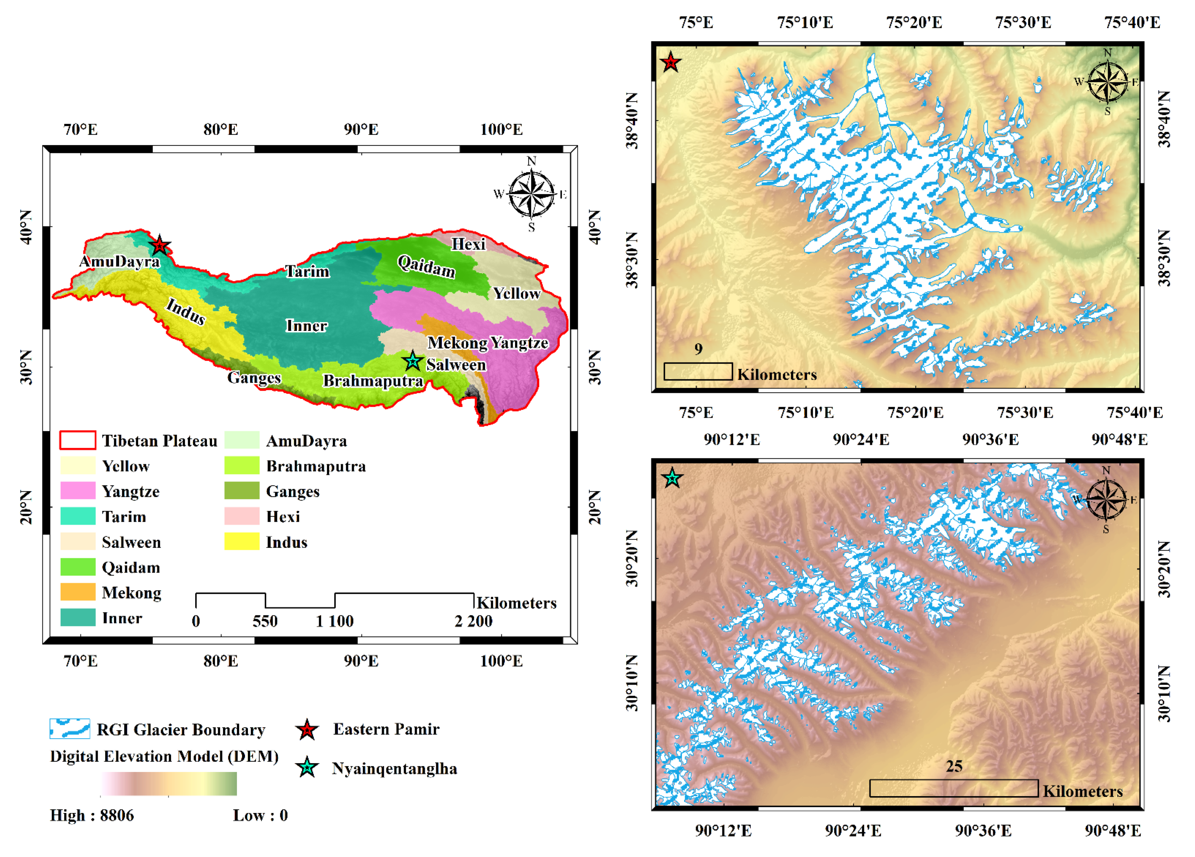
2.1. Research Area

In HMA, mountain glaciers can also be divided into continental glaciers and maritime glaciers. Continental glaciers are mainly developed under continental climatic conditions, and they mainly depend on the cold storage conditions provided by the cold and severe climate to survive, with a low glacier movement rate and a high elevation of terminus. Continental glaciers are one of the main types of glaciers in China, constituting approximately 78% of the country’s glaciers [12]. Maritime glaciers (also known as monsoonal maritime glaciers) are mainly developed in climatic zones influenced by a monsoonal climate and are one of the main types of glaciers in China [12]. They are mainly characterized by high accumulation, high ablation, rapid movement, and a very sensitive response to climate change.

Eastern Pamir [11,56] (Figure 1) mainly comprises mountains and valleys in the northwest–southeast direction. The terrain is complex, with an average elevation of around 5500 m. The highest peak, Kongur Tagh Mountain, is approximately 7649 m above sea level [57]. The large-scale glaciers of the Eastern Pamir are mainly concentrated in the two areas centered on the Muztagh Ata–Kongur Tagh in the southeast. The other mountains host primarily small-scale glaciers, which are continental glaciers.

The glaciers in the western section of the Nyainqentanglha [58,59] Mountains (Figure 1) are continental glaciers. The eastern part of the mountain range is significantly affected by the southwestern Indian Ocean monsoon, with a great deal of precipitation, low snow line, and concentrated glaciers. It is the largest maritime glacier concentration area in China and one of the strongest centers of glacial action in the middle and low latitudes of the earth.

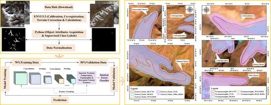
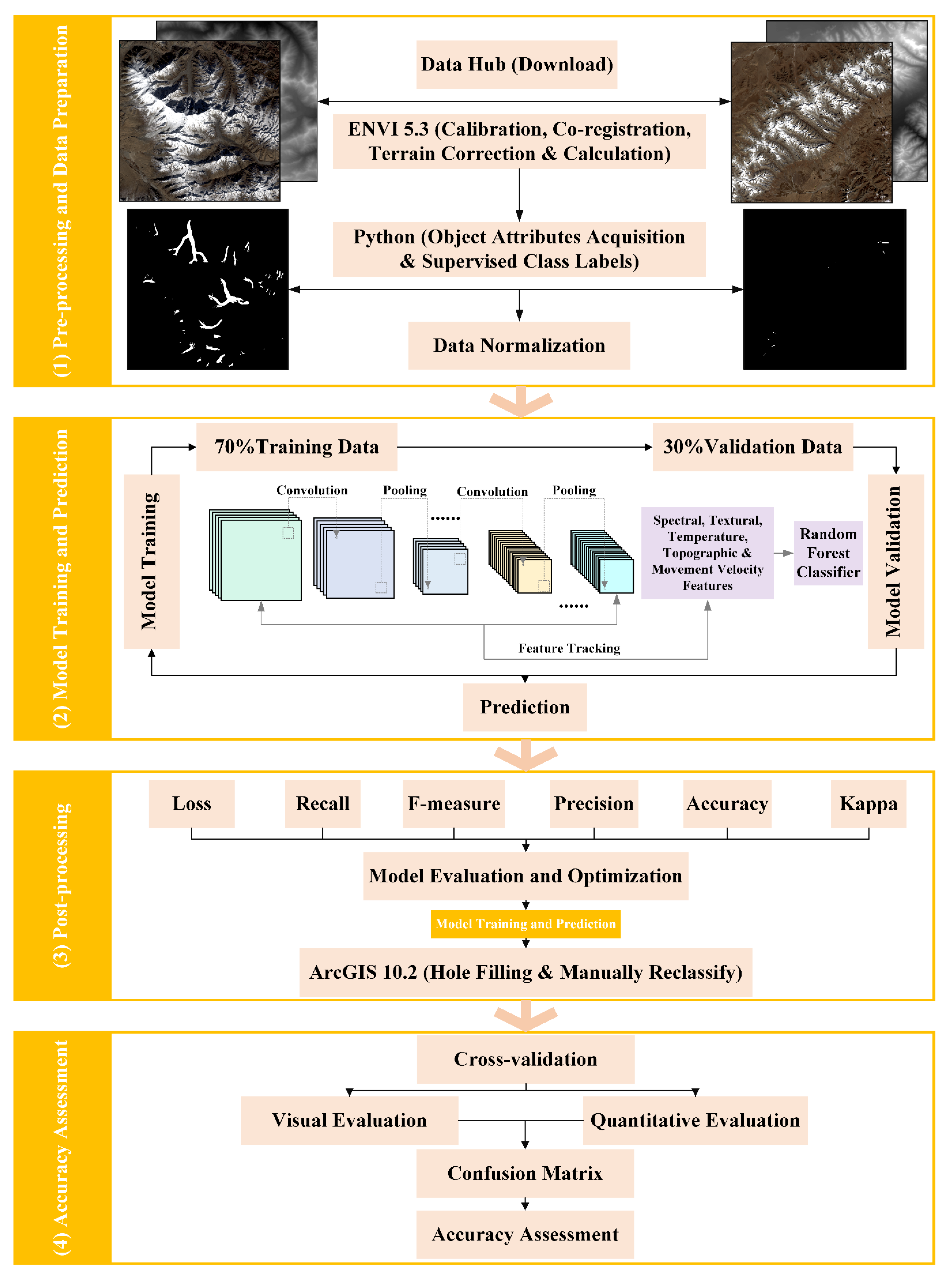
2.2. Dataset Acquisition and Pre-Processing

Summer is usually the best season to identify glaciers from images because most seasonal snow melts during this season. However, for the HMA area, owing to the differences in climate and topography between the various basins, the acquisition time of the images cannot be generalized [60]. With the help of historical Google Earth images, we selected images with as little cloud coverage and seasonal snow as possible from the images that match the best seasons as our final data set, as detailed in

Table 1. Data used for glacier mapping.

Data	Acquisition Time (YearMonthDay)	Bands	Resolution (m)
Landsat 8	Eastern Pamir 20171020	OLI (B1, B2, B3, B4, B5, B6, and B7)	30
	Nyainqentanglha 20171023
Landsat 8	Eastern Pamir 20171020	TIRS (B10)	100
	Nyainqentanglha 20171023
ASTER GDEM V2	2009	Estimation of terrain elevation	30
The Randolph Glacier Inventory: Version 6.0 (RGI 6.0)	2017	Estimation of glacier area change
The second glacier inventory dataset of China (CGI2)	2006–2011	Estimation of glacier area change
A dataset of glacier inventory of West China in 2018 (WCGI)	2018	Estimation of glacier area change

. Additionally, Landsat 8 scenes of World Reference System 2 both used for Eastern Pamir (path 149 and row 33) and Nyainqentanglha (path 138 and row 39) can be freely downloaded from https://earthexplorer.usgs.gov/, (accessed on 2 July 2021) and the Geospatial Data Cloud site (http://www.gscloud.cn), (accessed on 2 July 2021) for ASTER GDEM V2 data. The second glacier inventory dataset for China was obtained from the Institute of Tibetan Plateau Research, the Chinese Academy of Sciences. Further, the Randolph Glacier Inventory is available from GLIMS (https://www.glims.org/), (accessed on 2 July 2021). A dataset of the glacier inventory of West China in 2018 is available from http://www.csdata.org/p/551/, (accessed on 2 July 2021). These inventory datasets were applied to estimate the effectiveness of the glacier boundary detection, based on the RF–CNN algorithm.

Before the classification of glaciers, the original remote sensing data must be pre-processed. The specific steps of this process include the following:

(1)

Perform radiometric and atmospheric correction on the spectral data of Landsat 8 images.

(2)

The band calculation tool of the ENVI software is used to normalize the data of each band, and the normalized difference vegetation index (NDVI) [61,62], normalized difference water index (NDWI) [63,64], and normalized difference snow index (NDSI) [26,65] are calculated. It also identifies the coastal/aerosol, red, green, and blue bands, along with the near-infrared (NIR) and mid-infrared (SWIR-1 and SWIR-2) bands. The texture features (mean) [11] based on spectral data are then calculated by the statistical method of the grey-scale co-occurrence matrix (GLCM) proposed in the early 1970s by R. Haralick et al. [66]. Temperature characteristics (LST) are automatically obtained by identifying image metadata information through the surface temperature inversion tool of the ENVI software and obtaining atmospheric profile parameters. The glacier movement data are obtained by tracking the displacement of the glacier surface features between the two phases of Landsat 8 images based on the image cross-correlation method of frequency domain transformation in the COSI-Corr software package [67]. The calculation of terrain features is based on DEM data to obtain the elevation, slope, aspect, and shaded relief. The above feature data (spectral features + textural features + temperature features + topographic features + movement velocity features) are separately output as a grayscale image, which results in 23 grayscale images.

(3)

Load the 23 grayscale images and create a new debris-covered glacier vector file according to the visual interpretation method based on 23 grayscale images showing the extent of glaciers through ArcGIS software. The processed glacier vector file is binarized to finally obtain a label file of the remote sensing image glacier distribution.

(4)

Utilize the OpenCV-Python library function in Python to read the 23 processed grayscale images and corresponding label files, and use the sliding window to crop the images; use the ‘imgaug’ library function to obtain the expanded dataset of all the cropped images according to the data enhancement method by operations such as panning and flipping; finally, through linear mapping of each dimensional feature into the target range [−1, 1], the normalized dataset is obtained, and all the normalized images are divided to obtain a training set, a validation set, and a test set.

2.3. Input Feature Analysis for Classification

The velocity of glacier movement is a key factor for understanding the nature of glaciers and quantifying glacier changes, and it is also an important metric for glacier dynamics [4]. A frequency domain algorithm was used in Landsat 8 OLI images (panchromatic band, 15 m resolution) taken approximately one year apart between the two periods to calculate the correlation coefficient in the COSI-Corr software, with the reference window set to 128 and the search window set to 32, to obtain the glacier movement velocity data (Figure 2). Figure 2 shows the velocity for debris-covered glaciers in the study area. The Karayaalak Glacier conforms to the characteristics of a fast-moving glacier, where the lateral branches move fast (particularly the western) while the main glacier trunk has a much lower speed [68], which is mainly due to the many small supraglacial lakes in the east branch of the Karayaalak Glacier (Figure 3). It is generally believed that the supraglacial lakes accelerate glacier movement [15]. The surface velocity of the tongue part of the Qimgan Glacier does not conform to the characteristics of normal glacier flow. According to Google Earth images and a study conducted by Scherler [69], this area is a dead ice area covered in surface debris (Figure 3), indicating that the deep surface debris-covered area may no longer be active. It should be noted that the feature tracking of steep-slope areas is affected by their topography and other factors, leading to significant uncertainty. In summary, although the glacier movement velocity is useful to ascertain the surface debris area since the glacier movement velocity does not conform to a uniform law, we also need to refer to other variables to fully identify and extract debris-covered glacier areas.

The correlations shown in Figure 4 are the correlation coefficients of the variables for the classification of debris-covered glaciers. When the correlation coefficient p is greater than 0.05, the relationship between the two is strong. According to an analysis by Lu [11], the mean in image texture features plays a decisive role in the mapping of glaciers. Therefore, to avoid model overfitting, only the mean is used here to represent texture features. According to saliency relationships, it can be seen in Figure 4 that—among the classification variables of debris-covered glaciers—SWIR1, SWIR2, and their respective mean values have a strong influence. Further, NDVI, NDSI, and LST also play important roles. This is primarily because the optical band plays a crucial role in all variables, and the exponential features and texture features generated by it respond to it simultaneously. Terrain features and glacier movement velocity features are equally important and play an auxiliary role in the classification of debris-covered glaciers. The importance of these two types of features takes into account the control of topographic factors, so they are also related. We calculated the eigenvector value relating to the feature vector, which represents the contribution of each variable to the debris-covered glacier classification. We observe that the eigenvalues of almost all variables are positive. The greater the positive value of strong reflection, the better the effect of strong absorption. This is in line with the requirements of debris-covered glacier classification.

3. Methodology

In traditional remote sensing image segmentation methods, feature extraction and model establishment are achieved manually [70,71]. However, for the segmentation of specific targets in remote sensing images, the object-relational mapping between the feature space and the segmentation target is high-dimensional and strongly nonlinear. Therefore, effectively constructing this type of model through manual methods is difficult. To this end, various learning-based remote sensing image segmentation methods can help to undertake high-dimensional, strongly nonlinear mapping through sample learning.

3.1. Random Forest Classification

The random forest (RF) remote sensing image segmentation method is a classifier built based on multiple decision trees. Each decision tree classifies the sampled data set using the selected features and finally combines the classification results of each decision tree through a voting mechanism [49]. The entire construction process of the RF model uses randomly selected training samples and input features to generate and train each decision tree. After training, the test set samples are applied to the already trained classification model, and each decision tree will obtain the corresponding classification results. These results are recorded through voting, and the category with the most votes will be the final result.

Glacier mapping using RF models to achieve target segmentation of glacier remote sensing images includes the following:

(1)

Decompose the input Landsat 8 images and DEM data; extract the data’s spectral features, index features, texture features, temperature features, topographic features, and glacier movement speed features to obtain a 24-dimensional data set.

(2)

Randomly scramble the data set and construct attribute sets separately. Select 70% of the samples as the labeled sample set, and the rest are unlabeled sample sets. Use the same loss function for the unlabeled and labeled samples to build the initial RF model.

(3)

Initialize the number of training iterations, select a certain number of label samples to train the classifier, take all the unlabeled samples with high confidence values, and give each label a value. Then, add it to the label set and update the label sample set. The latter label sample set is used as the training set for the semi-supervised training of the RF model to obtain a new RF model.

(4)

By introducing unlabeled data and adding all unlabeled sample data to the optimization goal, the initial value of the data misclassification rate of the overall model is given to control the optimization. When the misclassification rate of the entire out-of-bag data set is zero, the optimal RF model is obtained.

(5)

According to the category label matrix, each pixel of the glacier data based on remote sensing images and digital elevation models is classified; the classified image is output, and the classification accuracy rate is calculated.

The technical process of debris-covered glacier classification based on the RF classifier is shown in Figure 5.

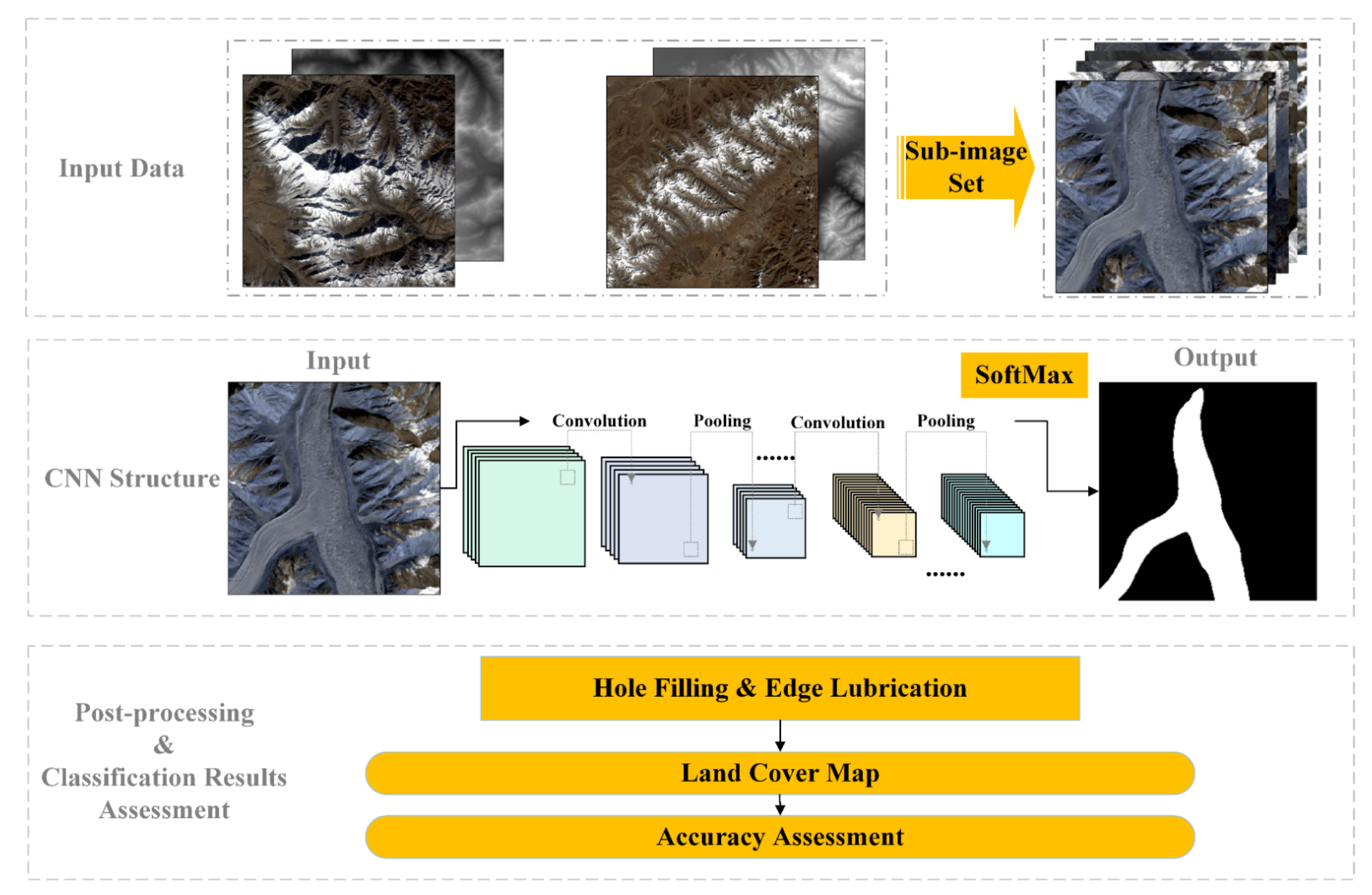
3.2. Convolutional Neural Network Classification

The convolutional neural network (CNN) remote sensing image segmentation method performs semantic segmentation of an image—that is, it classifies each pixel. Therefore, its basis is still the image classification problem based on the combination of the scale space and the spectral relationship of the remote sensing image feature extraction [72]. A CNN primarily comprises a convolutional layer and a pooling layer. The essence of a CNN is to construct multiple filters that can extract data features, and to extract these data structure features through convolution and pooling operations. Convolutional layer neurons extract features by acquiring local information and then combining higher layers to obtain global information. The pooling layer is based on the convolutional layer, which down-samples the extracted data features to improve the generalization of the extracted data.

Glacier mapping using the CNN model to achieve the target segmentation of glacier remote sensing images includes the following steps:

(1)

Use the ‘TensorFlow’ and ‘Keras’ packages in Python to build a CNN framework to construct a remote sensing image glacier segmentation model based on deep learning [73,74]. The glacier segmentation model based on remote sensing images has 24 inputs as training samples, including 23 grayscale images and 1 corresponding label file.

(2)

According to the calculation performance of the computer’s graphics card and the number of model parameters, set the training batch size = 128 and learning rate = 0.001, use the training function and the training set to iteratively train the remote sensing image glacier segmentation model, and use the validation set and test set to verify and test the remote sensing image glacier segmentation model after each round of training, respectively. When the remote sensing image glacier segmentation model converges, save the trained remote sensing image glacier segmentation model.

(3)

After outputting the segmentation results of the trained remote sensing image glacier segmentation model, the segmentation results are fine-tuned using the guided filter (GF) [75] and conditional random field (CRF) model [76]. Among them, GF uses the label file as a guide map, and uses the original image as the input image to optimize the boundary of the glacier extraction results to eliminate salt-and-pepper noise. The binary potential function in the CRF constrains the color and position between any two pixels, making it easier for pixels with similar colors and adjacent positions to have the same classification. Further, edges are smoothed according to the smoothness between adjacent pixels.

The technical process for debris-covered glacier classification based on an RF–CNN classifier is shown in Figure 6.

3.3. RF–CNN Classification

Relying on only one classifier cannot guarantee the best classification results. Leveraging the corresponding advantages of RF and CNN models, a combination of these two strategies has the potential to improve the final classification performance. Therefore, we build an RF–CNN composite classifier herein.

Glacier mapping using the RF algorithm based on the CNN model (RF–CNN) to achieve target segmentation of glacier remote sensing images includes the following steps:

(1)

Create a training dataset for the study area, and use samples and sample labels as the training data set;

(2)

First, establish a CNN model; then, use the samples and sample labels in step (1) to train the model, and save the model for later use;

(3)

Use the CNN model in step (2) to extract the feature layers of the study area—that is, extract the deep features;

(4)

Extract the shallow features of Landsat 8 images and DEM in the study area, including spectral features, index features, texture features, temperature features, topographic features, and glacier movement speed features;

(5)

Perform multi-feature combination for the deep features extracted in step (3) and the shallow features extracted in step (4);

(6)

Use RFs to perform semantic segmentation on the combined features in step (5) to achieve glacier segmentation based on remote sensing images.

This study uses a two-dimensional convolution (Conv 2D) method to process the data set, and uses a sliding window crop with a repetition rate of 0 to crop the experimental data into data blocks and input them into the network. Subsequently, geometric transformations are performed on the training data (including horizontal, vertical, and diagonal flipping). Data enhancement operations are then used to automatically extract various features of the remote sensing images. Before pooling (MaxPooling 2D), an activation function is needed to increase the nonlinear characteristics of the model. The activation function utilizes the SoftMax function to improve the generalization ability of the network. The technical process of debris-covered glacier classification based on the RF–CNN classifier is shown in Figure 7, and the RF–CNN model parameter settings are given in

Table 2. RF–CNN model parameter settings.

Name	Explanation	Value
N_estimators	Maximum number of weak learners (decision trees).	1000
Criterion	Criteria for evaluating features when dividing decision trees. The options are ‘Gini’ for Gini impurities and ‘entropy’ for information gain.	Gini
Max_features	Maximum number of features considered when dividing decision trees.	None
Max_depth	Decision tree maximum depth.	None
Min_samples_split	Minimum number of samples required for internal node subdivision.	10
Min_samples_leaf	Minimum number of samples for leaf nodes.	1
Training Threshold Contribution	Determines the contribution of internal weights related to the activation node level.	0.9
Training Rate	The larger the parameter value, the faster the training. speed, but it also increases the swing or causes the training result to not converge.	0.2
Training Momentum	The function of this parameter is to cause the weight to change in the current direction.	0.9
Training RMS Exit Criteria	At this specific value of RMS error, the training should stop.	0.1
Number of Hidden Layers	The number of hidden layers used.	1
Number of Training Iterations	The number of iterations used for training.	1000

.

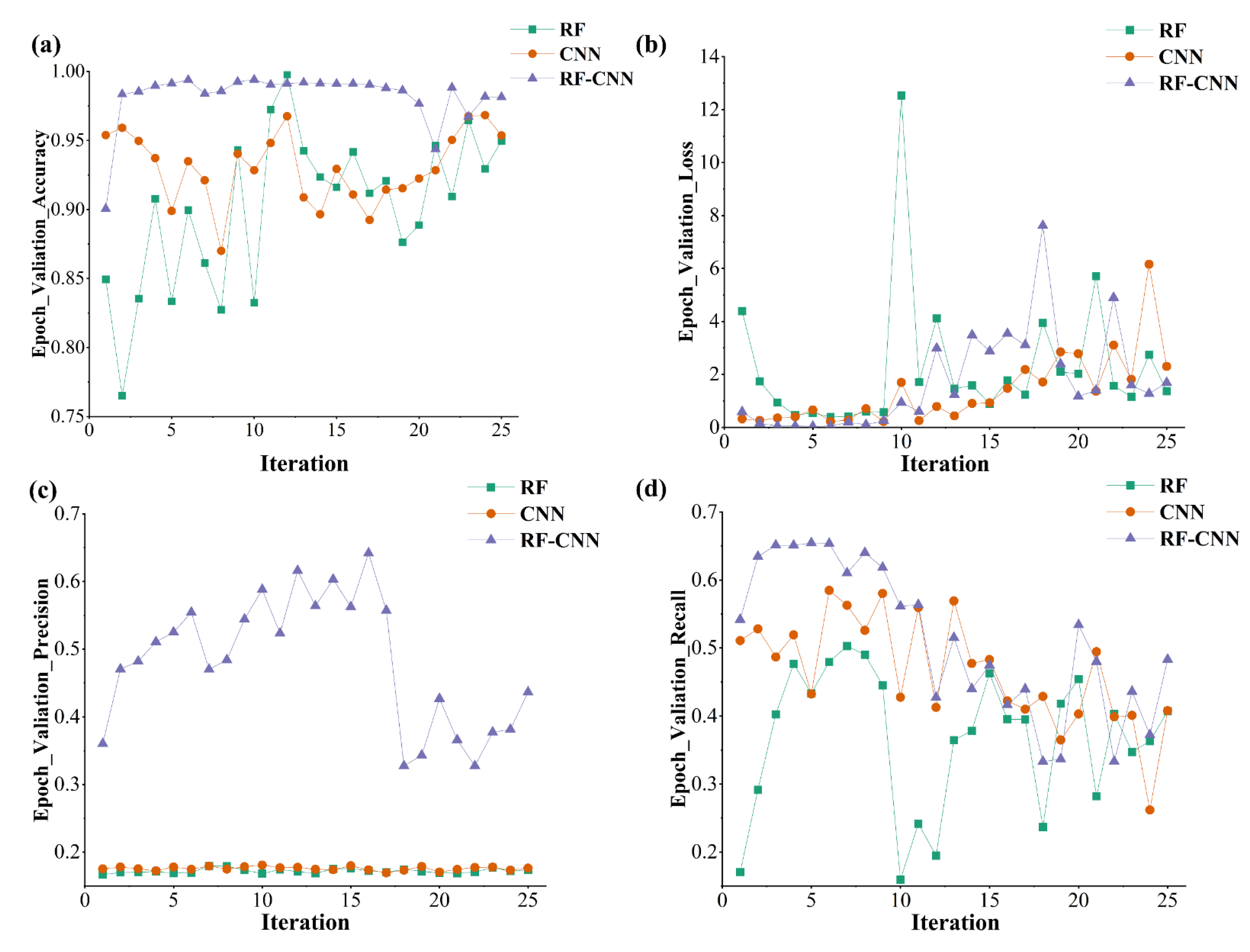
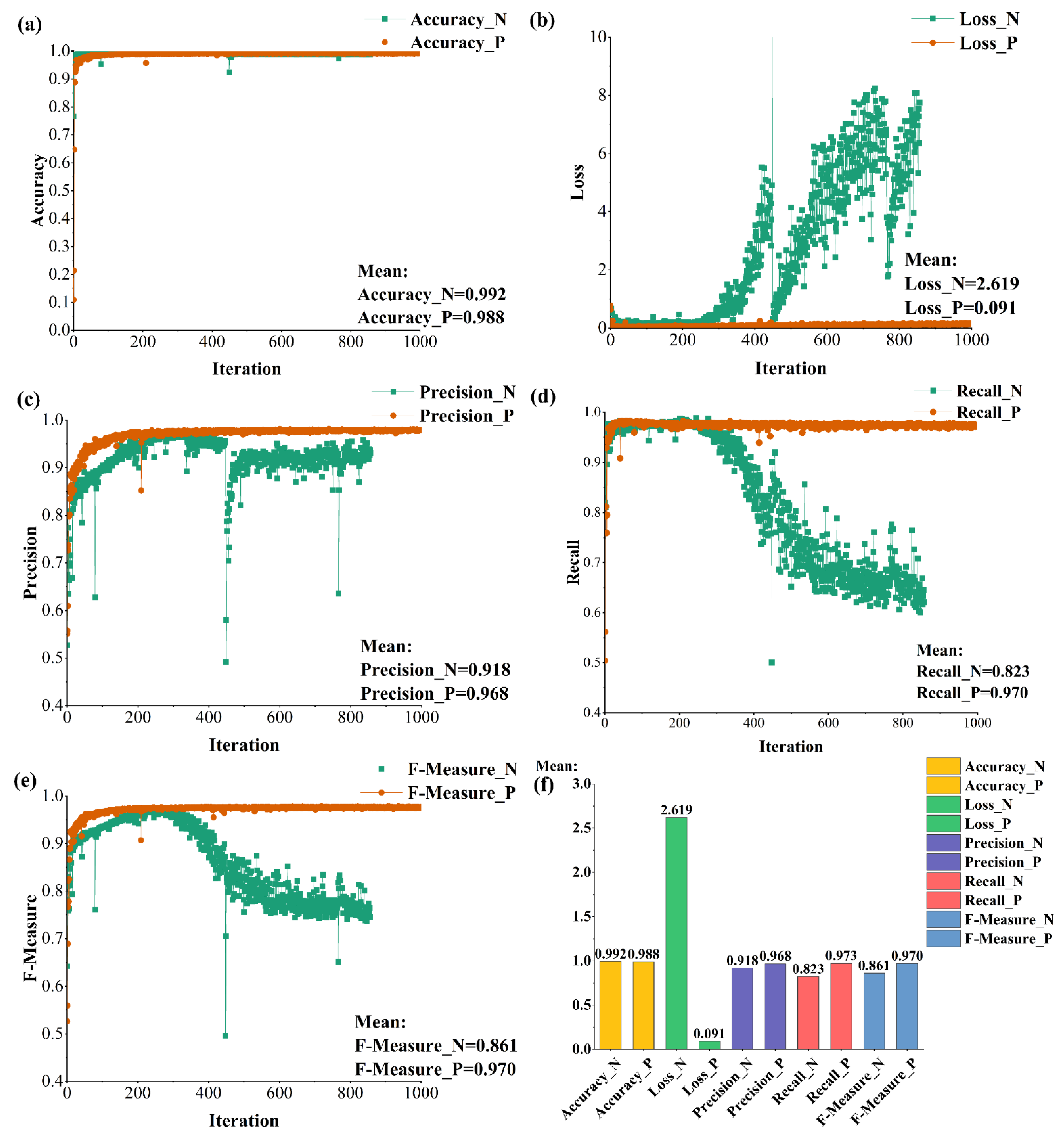
3.4. Selection of Classification Metrics

The deep learning evaluation standard consists of TP, FN, FP, and TN (

Table 3. Deep learning evaluation criteria.

Confusion Matrix		Prediction
		1	0
Real	1	TP	FN
	0	FP	TN

).

T = True and F = False, indicating whether the prediction is correct; P = Positive and N = Negative, indicating whether the prediction result is positive or negative.

TP = True Positive: the number of positive classes predicted by the actual positive class; FN = False Negative: the number of negative classes predicted by the actual positive class.

FP = False Positive: the number of positive classes predicted by the actual negative class; TN = True Negative: the number of negative classes predicted by the actual negative class.

The following formulas (Equations (1) and (2)) help to calculate the expected value through the error matrix:

$$\begin{array}{c}T{P}_{expected}=\frac{\left(TP+FP\right)\times \left(TP+FN\right)}{TP+FP+TN+FN}\end{array}$$

(1)

$$\begin{array}{c}T{N}_{expected}=\frac{\left(TN+FN\right)\times \left(FP+TN\right)}{FP+TP+FN+TN}\end{array}$$

(2)

In remote sensing image segmentation, the recall rate, precision rate, and F-measure are commonly used as segmentation performance evaluation indicators [70,71]. The recall rate represents the ratio of pixels divided into glaciers to actual glacier pixels. A high recall rate indicates better glacier extraction; however, this value cannot discern whether the background is more likely to be mistakenly classified as a glacier. The precision rate represents the ratio of pixels that are correctly segmented into glaciers to all pixels that are segmented into glaciers, which indicates the accuracy of glacier segmentation without considering the background of remote sensing images. The F-measure is a comprehensive performance indicator that strikes a balance between the recall rate and precision rate. A higher F-measure value indicates that the recall rate is higher when the precision rate is higher, which means that the actual segmentation accuracy is higher. The specific experimental performance index calculation formula is shown in

Table 4. Performance metrics based on the error matrix.

Measure Name	Formula
Recall	$\mathrm{Recall}=\frac{TP}{TP+FN}$
Precision	$\mathrm{Precision}=\frac{TP}{TP+FP}$
Accuracy	$\mathrm{Accuracy}=\frac{TP+TN}{TP+TN+FN+FP}$
F-measure	$\mathrm{F}-\mathrm{Measure}=2\times \frac{\mathrm{Precision}\times \mathrm{Recall}}{\mathrm{Precision}+\mathrm{Recall}}$
Kappa	$\mathrm{Kappa}=\frac{\left(TP+TN\right)-\left(T{P}_{expected}+T{N}_{expected}\right)}{\left(TP+FP+TN+FN\right)-\left(T{P}_{expected}+T{N}_{expected}\right)}$

.

4. Results

We characterize the quality of model training using the recall, loss, precision, accuracy, and F-measure values of the batch, epoch, and epoch_valiation. Taking the same iteration 25 times as an example, it is found that the learning rate of the RF model is too low and the training time is too long. It is necessary to increase the learning rate and retrain the model. The CNN model performance dropped sharply initially, but it soon returned to its original level. In the later stages, the learning rate is too large, failing to fit the results adequately. Therefore, the learning rate should be reduced and the next few rounds of training should be retrained. By adjusting the hyperparameters of the RF–CNN model, optimization is achieved (Figure 8, Figure 9 and Figure 10). Each sample in a single-label classification task has only one category. If the category is predicted, the classification is correct, and if it is not predicted, it is recorded as a classification error. Therefore, the most intuitive indicator is accuracy, which denotes the accuracy rate. The accuracy rate of the models that we trained (RF, CNN, and RF–CNN) is extremely close to 100% (Figure 8, Figure 9 and Figure 10), which directly indicates that the constructed model is suitable for the classification of debris-covered glaciers. Furthermore, the accuracy rate of the RF-CNN model is better than that of the other two models, which is in line with our expectations. When we iterate the data 1000 times, the root mean square (RMS) value begins to oscillate around 0.829, which means that the overfitting phenomenon has been greatly alleviated, and the model can obtain good generalization performance.

For automatic glacier classification based on remote sensing images, the results usually contain many small spots or holes. To improve the accuracy of image classification, we eliminated or reclassified these small holes. The distribution map of the debris after classification is shown in Figure 11.

The classification performance of the classifier is evaluated using selected validation samples. The validation sample was selected based on the Landsat 8 images listed in Table 1. Pixel-based classification assessment indicators include the overall accuracy, Kappa coefficient, user’s accuracy, and producer’s accuracy, based on the classification confusion matrix [77]. We calculate the accuracy of classification by comparing the position of each test pixel with its corresponding position in the classification image, the results of which are given in

Table 5. Accuracy assessment.

Eastern Pamir	RF	CNN	RF-CNN
Overall Accuracy	97.60%	96.34%	98.14%
Kappa Coefficient	0.96	0.95	0.97
User’s Accuracy	91.59%	87.96%	97.90%
Producer’s Accuracy	97.17%	98.69%	98.33%
Nyainqentanglha
Overall Accuracy	99.31%	99.06%	97.62%
Kappa Coefficient	0.98	0.97	0.94
User’s Accuracy	92.53%	78.75%	90.60%
Producer’s Accuracy	98.86%	97.53%	74.54%

. In general, the RF method performs best overall, not the RF-CNN method. Both its Kappa coefficient and user/producer’s accuracy is higher. However, the RF-CNN method can provide a plausible reference value for the extraction of debris-covered glaciers. The Eastern Pamir and Nyainqentanglha regions are obviously different, and we pay special attention to the relational mapping between the intensity of the debris coverage and the construction of the machine learning model to compare the size of the debris coverage and the quality of the model training in different areas.

The results of model training differ slightly from sample to sample. In Eastern Pamir, the total area occupied by the glaciers was 605.117 km², of which 85.398 km² was covered in debris and 519.718 km² was not. Debris-covered glaciers in Nyainqentanglha were mainly distributed between 4000 and 6000 m, with an area of approximately 126.736 km². The possible reason for this is that the sample sizes in Eastern Pamir and Nyainqentanglha are different. Eastern Pamir was involved in the training and testing of 7499 samples, while Nyainqentanglha was involved in the training and testing of only 3099 samples. The fact is that the debris coverage rate in Nyainqentanglha is indeed not as high as that in Eastern Pamir. It is clear that the size of the sample directly determines the result (Figure 12). In areas with more surface debris, sufficient labels and sample data are provided, and the trained model performs better. From the surface debris data, Eastern Pamir provided more training data than Nyainqentanglha in this experiment, so the results for the former are more accurate.

Furthermore, the cloud coverage, snow coverage, and terrain shadow coverage of the glacier surface are all specific indicators that affect the classification results. These factors are mainly determined by the quality of the image, which is determined by the time taken by the sensor to acquire the image, illumination conditions, and climatic conditions. We have mitigated the influence of cloud coverage when selecting remote sensing images (the cloud coverage is less than 10%), primarily to eliminate the clouds over the glacier and obtain its true spectral properties. Further, our study is focused on summer, when the snow coverage is the lowest in the year. Terrain shadow coverage is mainly determined by the sun azimuth and sun altitude. Particularly for mountain glaciers with undulating terrain, such as Eastern Pamir and Nyainqentanglha, the phenomenon of shadows obscuring the glacier can only be reduced, not eliminated. Future research should focus on the impact of these shadow areas on automatic glacier extraction.

5. Discussion

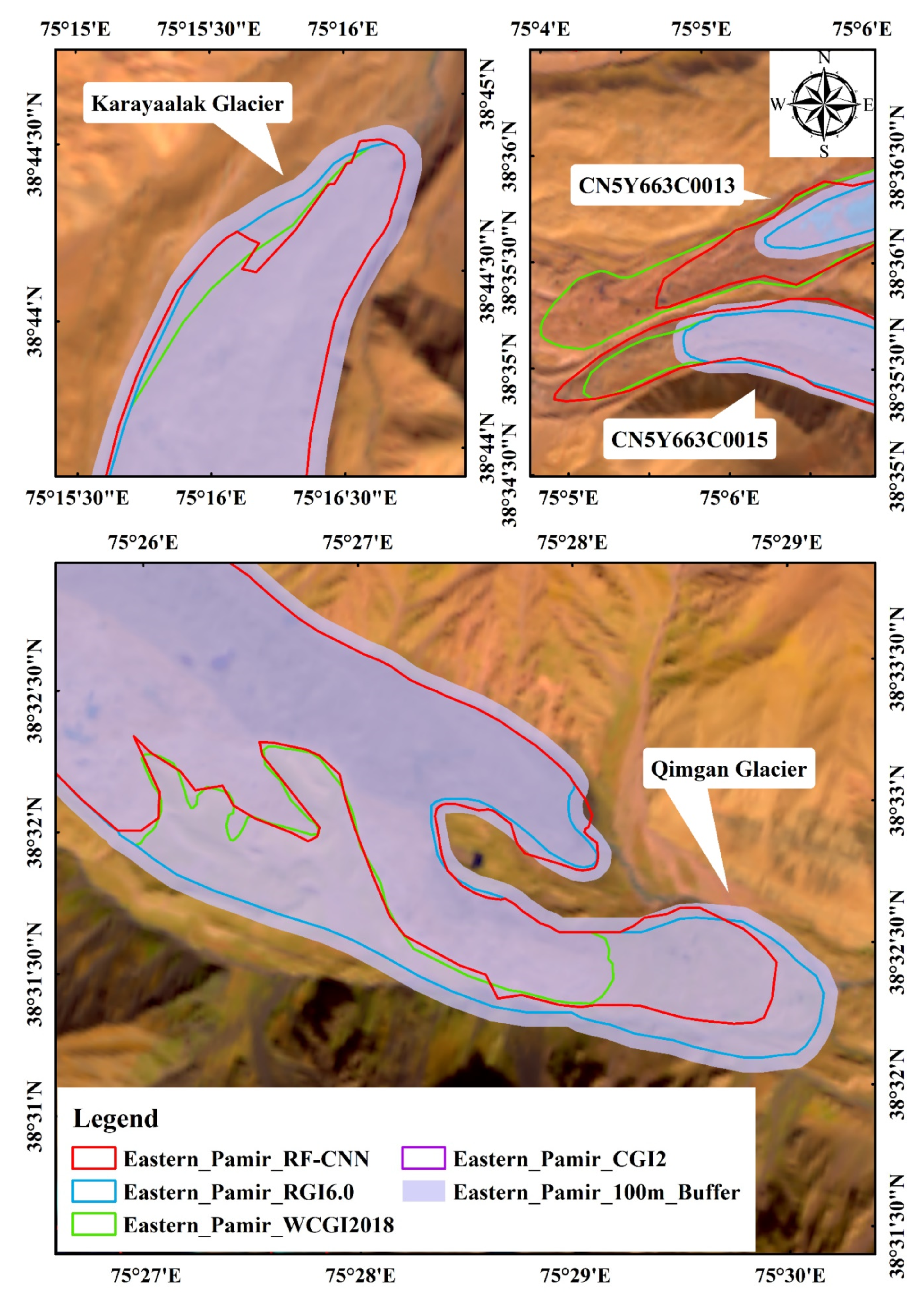
5.1. Comparison with Existing Methods and Inventories

We use the three kinds of glacier inventory data (CGI 2, RGI 6.0, and WCGI 2018) as the analysis object of the experimental results.

Firstly, the scopes of the two types of glacier inventory data (RGI 6.0 and CGI2) are nearly the same in Eastern Pamir and Nyainqentanglha, so we primarily use RGI 6.0 for visual analysis, which considers the reference value of RGI in worldwide cryosphere research. According to statistics, WCGI2018 shows 461.448 km² of debris-covered glacier area in Eastern Pamir, but 462.521 km² of debris-covered glacier is found in RGI 6.0 and CGI2. The area of these debris-covered glaciers—for the most part—does not change; only a few glaciers exhibit slight changes (an area of less than 3 km²) owing to the greater response of large glaciers to the climate and terrain [1,60]. Further, WCGI2018 shows 6.128 km² of debris-covered glacier in Nyainqentanglha, but 6.197 km² of debris-covered glacier is found in RGI 6.0 and CGI2. Considering that WCGI2018 is also a manually drawn glacier contour based on CGI2, there is not much difference in terms of value; any variations could be due to human error caused by technical personnel’s subjective understanding of glaciers.

Secondly, when we conduct quantitative analysis, we randomly select 19 debris-covered glaciers as the research object (

Table 6. Comparison of the debris-covered glacier area derived from the automatic extraction algorithms and from other inventories.

Glacier Name	Existing Methods and Inventories (km2)
	RGI 6.0	CGI 2	WCGI 2018	STD.	Mean	RF-CNN
G075254E38623N	115.162	115.162	114.833	0.155	115.052	115.588
G075133E38690N	11.557	11.557	11.481	0.036	11.532	11.699
G075146E38607N	17.207	17.207	17.420	0.100	17.278	17.904
G075262E38523N	10.365	10.365	10.599	0.110	10.443	10.846
G075400E38636N	9.934	9.934	9.853	0.038	9.907	9.934
G075339E38560N	86.631	86.631	83.998	1.241	85.753	84.859
G075304E38449N	22.950	22.950	22.914	0.017	22.938	23.192
G075321E38480N	26.468	26.468	26.468	0	26.468	26.469
G075457E38631N	13.901	13.901	13.882	0.009	13.895	13.930
G075486E38594N	9.346	9.346	9.464	0.056	9.385	9.519
G090600E30388N	27.354	27.354	27.298	0.026	27.335	27.417
G090618E30355N	7.133	7.133	7.105	0.013	7.124	7.229
G090071E29968N	4.762	4.762	4.668	0.044	4.731	4.672
G090039E29949N	3.048	3.048	2.943	0.049	3.013	3.051
G090040E29912N	5.444	5.444	5.438	0.003	5.442	5.717

). We used an evaluation tool named the ‘round robin’ method, proposed by Paul [78], to compare the area of debris-covered glaciers from RGI 6.0, CGI 2, and WCGI 2018 data with our RF-CNN results, taking into consideration that there are objective deviations in the judgment criteria of the three types of glacier inventory data. Finally, the average areas of the above three inventories are calculated as the criteria for evaluating the RF-CNN model, and the standard deviation of the glacier area is used as an indicator to measure the change in glacier area. In general, the area of the glacier trained by the RF-CNN model is larger than the area of the glacier inventory data of the above three datasets. The closer the standard deviation of the glacier area is to 0, the less the change in glacier area; this trend often appears in the small glaciers evaluated in Table 6. This is because large glaciers respond more severely to the combined effect of climate and topography than small glaciers [7,69].

Thirdly, taking Eastern Pamir as an example (Figure 13), the glacier boundary of RGI 6.0 is used as the visual judgment standard, and a buffer of 100 m is used as the error interval to identify the accuracy of RF-CNN for glacier extraction. We select four debris-covered glaciers (the Karayaalak Glacier, CN5Y663C0013, CN5Y663C0015, and the Qimgan Glacier) to demonstrate the performance of the RF-CNN model. The results obtained in this paper are all within the range of the buffer—that is, within the range of error. Regarding the Karayaalak Glacier, it is mentioned in the literature that there is no advancement at the terminus [68], which is consistent with our results. The CN5Y663C0013 and CN5Y663C0015 glaciers have significant glacier surges, which closely matches the results of WCGI 2018. This also implies that glacier extraction based on machine learning can support research into glacier advancement. The key problem when analyzing the Qimgan Glacier is the detection of the active and inactive debris-covered glaciers. Figure 3 shows the presence of dead ice at the end of the Qimgan Glacier. The overall velocity of the dead ice is very small, and it is difficult to visually interpret through remote sensing images. The glacial boundaries of RGI 6.0 and CGI2 both contain all portions of the debris area, but it is obvious that WCGI 2018 includes a part of the dead ice. However, Figure 13 shows that the integration of multiple remote sensing image features can accurately extract the debris area, irrespective of whether there is dead ice in the debris area.

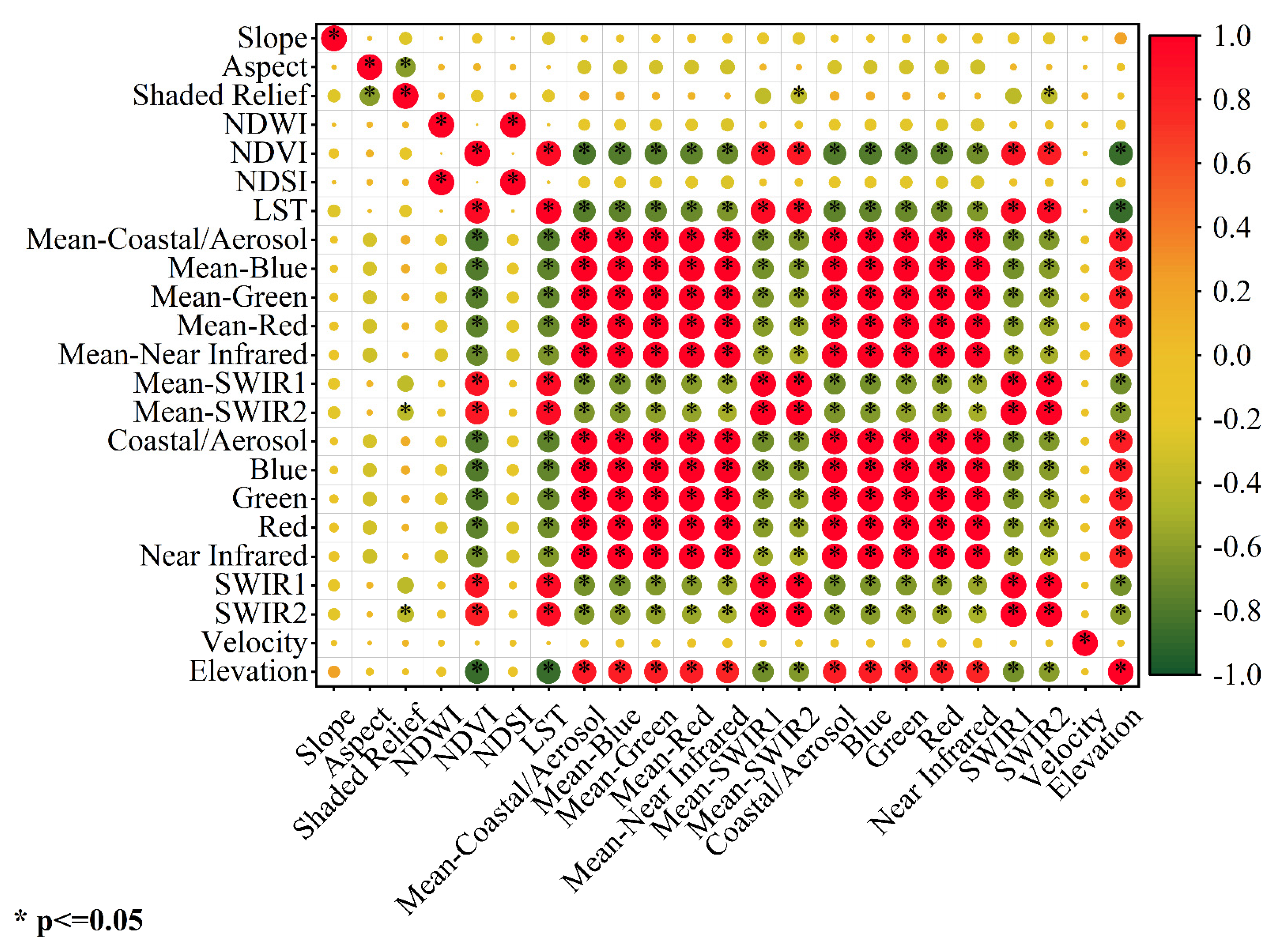
5.2. Feature Analysis

The correlation coefficient method assigns weights based on the repetitiveness of information between characteristic variables. In categorical data, there is a certain correlation between the selected feature variables. The correlation coefficient method not only avoids allocating excess weights to certain aspects of the data due to data duplication but also objectively reflects the importance of the feature variables [79]. Although the values of correlation coefficients obtained after model training differ, they all exhibit a consistent trend, as shown in Figure 14, Figure 15 and Figure 16. It is important to note that positive and negative values are equally important in the correlation coefficient graph. Among all the feature values, spectral features and texture features play a decisive role in the classification of debris-covered glaciers, because these two features are dependent on the spectral value of the optical image. Next, in terms of importance, are the three index characteristics (NDSI, NDVI, and NDWI) and LST, and the terrain features derived from the DEMs also had high correlation coefficients. The correlation between terrain features is not very significant. The glacier movement velocity is also affected by topographical factors, especially in the Eastern Pamir area, where the terrain is undulating [11], but its effect is also not significant.

It is worth noting that, although different studies on glacier mapping currently use different feature variables, these findings contribute in several ways to our understanding of detection at glacier boundaries and provide a basis for more in-depth research.

5.3. Limitations

The classification accuracy of the RF-CNN method is 98.14%, which is considered to be within the appropriate range [77], indicating that debris-covered glaciers can be extracted. However, this classification accuracy is affected—to a certain extent—by the model parameters and the accuracy of the sample set. The model parameters used in the experiment and the accuracy of the sample set are not discussed in detail. It is necessary to gradually explore the best glacier extraction model, the optimum parameters, and the best sample set in future work. Further, owing to the insufficient sample size in the Eastern Pamir (continental glaciers) and the Nyainqentanglha Mountains (maritime glaciers), the model trained using this deep learning framework is not suitable for complex mountain-shaded glaciers. A large number of compound glacier samples can be added to train the RF-CNN model to improve the accuracy for identifying mountain-shaded glaciers (continental glaciers and maritime glaciers). Because the glacier data set used in this experiment is not sufficiently large, the superiority of deep learning in comparison to traditional machine learning methods (such as RF and CNN) is not clear when processing large-scale sample sets. However, RF-CNN also has the advantage of high accuracy, where its accuracy does not depend on the choice of threshold. This means that it is a simple and feasible automatic method for glacier extraction.

6. Conclusions

This research uses Landsat and DEM as data sources, comparing and improving upon different classifier construction strategies (RF, CNN, and RF-CNN) to obtain multiple single-classifier outputs with certain differences, and then performing decision-level fusion of these outputs to obtain the final debris-covered glacier classification result. In general, the RF method performs best overall, while the RF-CNN method can provide a promising reference value for the extraction of debris-covered glaciers. This result helps to select the optimum classifier and improves the overall classification accuracy, striking a better balance between the classification effects of different methods.

The development of a machine learning method (RF-CNN) can effectively suppress classification uncertainty and further improve the generalization performance of the classifier is important. Combining various classification models also helped to mitigate the challenges regarding detection of the active and inactive debris-covered glaciers. Further, we analyzed the advantages and disadvantages of composite classification models in debris-covered glacier classification, and found that the performance of the machine learning model and the results of the final debris-covered glacier extraction are strongly dependent on the intensity of the debris coverage: the higher the proportion of surface debris coverage in the area, the more accurate the result, and vice versa. This can help to improve the glacier classification method and create conditions for rapid glacier inventory.

In subsequent research on glacier classification, more samples should be extracted to optimize the RF-CNN model. Based on the statistical characteristics of each pixel level of remotely sensed SAR images, this method of fine-tuning the network trained with optical images is not suitable for SAR image classification. In future work, the RF-CNN network model should be further improved to facilitate glacier classification while considering SAR images.

References

1. Paul, F.; Bolch, T.; Kääb, A.; Nagler, T.; Nuth, C.; Scharrer, K.; Shepherd, A.; Strozzi, T.; Ticconi, F.; Bhambri, R.; et al. The Glaciers Climate Change Initiative: Methods for Creating Glacier Area, Elevation Change and Velocity Products. Remote Sens. Environ. 2015, 162, 408–426. [Google Scholar] [CrossRef] [Green Version]
2. Zhou, Z.; Han, N.; Liu, J.; Yan, Z.; Xu, C.; Cai, J.; Shang, Y.; Zhu, J. Glacier Variations and Their Response to Climate Change in an Arid Inland River Basin of Northwest China. J. Arid Land 2020, 12, 357–373. [Google Scholar] [CrossRef]
3. Ye, Q.; Zong, J.; Tian, L.; Cogley, J.G.; Song, C.; Guo, W. Glacier Changes on the Tibetan Plateau Derived from Landsat Imagery: Mid-1970s–2000–13. J. Glaciol. 2017, 63, 273–287. [Google Scholar] [CrossRef] [Green Version]
4. Blöthe, J.H.; Halla, C.; Schwalbe, E.; Bottegal, E.; Trombotto Liaudat, D.; Schrott, L. Surface Velocity Fields of Active Rock Glaciers and Ice-debris Complexes in the Central Andes of Argentina. Earth Surf. Process. Landf. 2021, 46, 504–522. [Google Scholar] [CrossRef]
5. Zhao, Q.; Ding, Y.; Wang, J.; Gao, H.; Zhang, S.; Zhao, C.; Xu, J.; Han, H.; Shangguan, D. Projecting Climate Change Impacts on Hydrological Processes on the Tibetan Plateau with Model Calibration against the Glacier Inventory Data and Observed Streamflow. J. Hydrol. 2019, 573, 60–81. [Google Scholar] [CrossRef]
6. Regine, H.; Rasul, G.; Adler, C.; Cáceres, B.; Gruber, S.; Hirabayashi, Y.; Jackson, M. High Mountain Areas. In IPCC Special Report on the Ocean and Cryosphere in a Changing Climate; IPCC: Geneva, Switzerland, 2019. [Google Scholar]
7. Immerzeel, W.W.; Van Beek, L.P.; Bierkens, M.F. Climate Change Will Affect the Asian Water Towers. Science 2010, 328, 1382–1385. [Google Scholar] [CrossRef] [PubMed]
8. Immerzeel, W.W.; Lutz, A.F.; Andrade, M.; Bahl, A.; Biemans, H.; Bolch, T.; Hyde, S.; Brumby, S.; Davies, B.J.; Elmore, A.C.; et al. Importance and Vulnerability of the World’s Water Towers. Nature 2020, 577, 364–369. [Google Scholar] [CrossRef]
9. Nie, Y.; Pritchard, H.D.; Liu, Q.; Hennig, T.; Wang, W.; Wang, X.; Liu, S.; Nepal, S.; Samyn, D.; Hewitt, K.; et al. Glacial Change and Hydrological Implications in the Himalaya and Karakoram. Nat. Rev. Earth Environ. 2021, 2, 91–106. [Google Scholar] [CrossRef]
10. Liu, S.; Wu, T.; Wang, X.; Wu, X.; Yao, X.; Liu, Q.; Zhang, Y.; Wei, J.; Zhu, X. Changes in the Global Cryosphere and Their Impacts: A Review and New Perspective. Sci. Cold Arid. Reg. 2020, 12, 343–354. [Google Scholar] [CrossRef]
11. Lu, Y.; Zhang, Z.; Huang, D. Glacier Mapping Based on Random Forest Algorithm: A Case Study over the Eastern Pamir. Water 2020, 12, 3231. [Google Scholar] [CrossRef]
12. Liu, S.; Yao, X.; Guo, W.; Xu, J.; Shangguan, D.; Wei, J.; Bao, W.; Wu, L. The contemporary glaciers in China based on the Second Chinese Glacier Inventory. Acta Geogr. Sin. 2015, 70, 3–16. [Google Scholar] [CrossRef]
13. Zhao, L.; Ding, R.; Moore, J.C. Glacier Volume and Area Change by 2050 in High Mountain Asia. Glob. Planet. Chang. 2014, 122, 197–207. [Google Scholar] [CrossRef]
14. Zhang, Z.; Liu, S.; Jiang, Z.; Shangguan, D.; Wei, J.; Guo, W.; Xu, J.; Zhang, Y.; Zhang, S.; Huang, D. Glacier Variations at Xinqingfeng and Malan Ice Caps in the Inner Tibetan Plateau Since 1970. Remote Sens. 2020, 12, 421. [Google Scholar] [CrossRef] [Green Version]
15. Brun, F.; Wagnon, P.; Berthier, E.; Jomelli, V.; Maharjan, S.B.; Shrestha, F.; Kraaijenbrink, P.D.A. Heterogeneous Influence of Glacier Morphology on the Mass Balance Variability in High Mountain Asia. J. Geophys. Res. Earth 2019, 124, 1331–1345. [Google Scholar] [CrossRef]
16. Huo, D.; Chi, Z.; Ma, A. Modeling Surface Processes on Debris-Covered Glaciers: A Review with Reference to the High Mountain Asia. Water 2021, 13, 101. [Google Scholar] [CrossRef]
17. Miles, K.E. Hydrology of Debris-Covered Glaciers in High Mountain Asia. Earth Sci. Rev. 2020, 207, 103212. [Google Scholar] [CrossRef]
18. Wu, K.; Liu, S.; Xu, J.; Zhu, Y.; Liu, Q.; Jiang, Z.; Wei, J. Spatiotemporal Variability of Surface Velocities of Monsoon Temperate Glaciers in the Kangri Karpo Mountains, Southeastern Tibetan Plateau. J. Glaciol. 2021, 67, 186–191. [Google Scholar] [CrossRef]
19. Buchroithner, M.F.; Bolch, T. An Automated Method to Delineate the Ice Extension of the Debris-Covered Glaciers at Mt. Everest Based on ASTER Imagery. In Proceedings of the 9th International Symposium on High Mountain Remote Sensing Cartography, Graz, Austria, 14–22 September 2006. [Google Scholar]
20. Biddle, D. Mapping Debris-Covered Glaciers in the Cordillera Blanca, Peru: An Object-Based Image Analysis Approach. Master’s Thesis, University of Louisville, Louisville, KY, USA, 2015. [Google Scholar]
21. Racoviteanu, A.E.; Nicholson, L.; Glasser, N.F. Surface Composition of Debris-Covered Glaciers across the Himalaya Using Spectral Unmixing and Multi-Sensor Imagery. Cryosphere Discuss. 2021, 1–48. [Google Scholar] [CrossRef]
22. Fleischer, F.; Otto, J.; Junker, R.R.; Hölbling, D. Evolution of Debris Cover on Glaciers of the Eastern Alps, Austria, between 1996 and 2015. Earth Surf. Process. Landf. 2021, esp.5065. [Google Scholar] [CrossRef]
23. Xie, F.; Liu, S.; Wu, K.; Zhu, Y.; Gao, Y.; Qi, M.; Duan, S.; Saifullah, M.; Tahir, A.A. Upward Expansion of Supra-Glacial Debris Cover in the Hunza Valley, Karakoram, During 1990∼2019. Front. Earth Sci. 2020, 8, 308. [Google Scholar] [CrossRef]
24. Robson, B.A.; Bolch, T.; MacDonell, S.; Hölbling, D.; Rastner, P.; Schaffer, N. Automated Detection of Rock Glaciers Using Deep Learning and Object-Based Image Analysis. Remote Sens. Environ. 2020, 250, 112033. [Google Scholar] [CrossRef]
25. Zhang, J.; Li, J.; Menenti, M.; Hu, G. Glacier Facies Mapping Using a Machine-Learning Algorithm: The Parlung Zangbo Basin Case Study. Remote Sens. 2019, 11, 452. [Google Scholar] [CrossRef] [Green Version]
26. Huang, L.; Li, Z.; Zhou, J.M.; Zhang, P. An Automatic Method for Clean Glacier and Nonseasonal Snow Area Change Estimation in High Mountain Asia from 1990 to 2018. Remote Sens. Environ. 2021, 258, 112376. [Google Scholar] [CrossRef]
27. Pandey, A.; Rai, A.; Gupta, S.K.; Shukla, D.P.; Dimri, A.P. Integrated Approach for Effective Debris Mapping in Glacierized Regions of Chandra River Basin, Western Himalayas, India. Sci. Total Environ. 2021, 779, 146492. [Google Scholar] [CrossRef]
28. Yousuf, B.; Shukla, A.; Arora, M.K.; Bindal, A.; Jasrotia, A.S. On Drivers of Subpixel Classification Accuracy—An Example from Glacier Facies. IEEE J STARS 2020, 13, 601–608. [Google Scholar] [CrossRef]
29. Hoeser, T.; Bachofer, F.; Kuenzer, C. Object Detection and Image Segmentation with Deep Learning on Earth Observation Data: A Review—Part II: Applications. Remote Sens. 2020, 12, 3053. [Google Scholar] [CrossRef]
30. Hoeser, T.; Kuenzer, C. Object Detection and Image Segmentation with Deep Learning on Earth Observation Data: A Review-Part I: Evolution and Recent Trends. Remote Sens. 2020, 12, 1667. [Google Scholar] [CrossRef]
31. Mohammadimanesh, F.; Salehi, B.; Mahdianpari, M.; Gill, E.; Molinier, M. A New Fully Convolutional Neural Network for Semantic Segmentation of Polarimetric SAR Imagery in Complex Land Cover Ecosystem. ISPRS J. Photogramm. Remote Sens. 2019, 151, 223–236. [Google Scholar] [CrossRef]
32. Hoekstra, M.; Jiang, M.; Clausi, D.A.; Duguay, C. Lake Ice-Water Classification of RADARSAT-2 Images by Integrating IRGS Segmentation with Pixel-Based Random Forest Labeling. Remote Sens. 2020, 21, 1425. [Google Scholar] [CrossRef]
33. Abdollahi, A.; Pradhan, B.; Shukla, N.; Chakraborty, S.; Alamri, A. Deep Learning Approaches Applied to Remote Sensing Datasets for Road Extraction: A State-Of-The-Art Review. Remote Sens. 2020, 12, 1444. [Google Scholar] [CrossRef]
34. Dirscherl, M.; Dietz, A.J.; Kneisel, C.; Kuenzer, C. A Novel Method for Automated Supraglacial Lake Mapping in Antarctica Using Sentinel-1 SAR Imagery and Deep Learning. Remote Sens. 2021, 13, 197. [Google Scholar] [CrossRef]
35. Cordeiro, M.C.R.; Martinez, J.-M.; Peña-Luque, S. Automatic Water Detection from Multidimensional Hierarchical Clustering for Sentinel-2 Images and a Comparison with Level 2A Processors. Remote Sens. Environ. 2021, 253, 112209. [Google Scholar] [CrossRef]
36. Lv, X.; Ming, D.; Chen, Y.; Wang, M. Very High Resolution Remote Sensing Image Classification with SEEDS-CNN and Scale Effect Analysis for Superpixel CNN Classification. Int. J. Remote Sens. 2018, 40, 506–530. [Google Scholar] [CrossRef]
37. Marochov, M.; Stokes, C.R.; Carbonneau, P.E. Image Classification of Marine-Terminating Outlet Glaciers Using Deep Learning Methods. Cryosphere Discuss. 2020, 1–45. [Google Scholar] [CrossRef]
38. Nagapawan, Y.V.R.; Prakash, K.B.; Kanagachidambaresan, G.R. Convolutional Neural Network. In Programming with TensorFlow: Solution for Edge Computing Applications; Prakash, K.B., Kanagachidambaresan, G.R., Eds.; EAI/Springer Innovations in Communication and Computing; Springer International Publishing: Cham, Switzerland, 2021; pp. 45–51. [Google Scholar]
39. Bera, S.; Shrivastava, V.K. Analysis of Various Optimizers on Deep Convolutional Neural Network Model in the Application of Hyperspectral Remote Sensing Image Classification. Int. J. Remote Sens. 2020, 41, 2664–2683. [Google Scholar] [CrossRef]
40. Nijhawan, R.; Das, J.; Balasubramanian, R. A Hybrid CNN + Random Forest Approach to Delineate Debris Covered Glaciers Using Deep Features|SpringerLink. J. Indian Soc. Remote Sens. 2018, 46, 981–989. [Google Scholar] [CrossRef]
41. Xie, Z.; Haritashya, U.K.; Asari, V.K.; Young, B.; Bishop, M.P.; Kargel, J.S. Mapping Himalayan and Karakoram Glaciers Using Deep Learning Approach. AGU Fall Meet. Abstr. 2019, 2019, C51B-1272. [Google Scholar]
42. Xie, Z.; Haritashya, U.K.; Asari, V.K.; Young, B.W.; Bishop, M.P.; Kargel, J.S. GlacierNet: A Deep-Learning Approach for Debris-Covered Glacier Mapping. IEEE Access 2020, 8, 83495–83510. [Google Scholar] [CrossRef]
43. Xie, Z.; Haritashya, U.K.; Asari, V.K.; Young, B.W.; Bishop, M.P.; Kargel, J.S. Corrections to GlacierNet: A Deep-Learning Approach for Debris-Covered Glacier Mapping. IEEE Access 2020, 8, 136794. [Google Scholar] [CrossRef]
44. Liu, W.; Chen, X.; Ran, J.; Liu, L.; Wang, Q.; Xin, L.; Li, G. LaeNet: A Novel Lightweight Multitask CNN for Automatically Extracting Lake Area and Shoreline from Remote Sensing Images. Remote Sens. 2021, 13, 56. [Google Scholar] [CrossRef]
45. Petrovska, B.; Zdravevski, E.; Lameski, P.; Corizzo, R.; Štajduhar, I.; Lerga, J. Deep Learning for Feature Extraction in Remote Sensing: A Case-Study of Aerial Scene Classification. Sensors 2020, 20, 3906. [Google Scholar] [CrossRef]
46. Mohajerani, Y.; Wood, M.; Velicogna, I.; Rignot, E. Detection of Glacier Calving Margins with Convolutional Neural Networks: A Case Study. Remote Sens. 2019, 11, 74. [Google Scholar] [CrossRef] [Green Version]
47. Breiman, L. Random Forests. Mach. Learn. 2001, 45, 5–32. [Google Scholar] [CrossRef] [Green Version]
48. Pal, M. Random Forest Classifier for Remote Sensing Classification. Int. J. Remote Sens. 2005, 26, 217–222. [Google Scholar] [CrossRef]
49. Belgiu, M.; Drăguţ, L. Random Forest in Remote Sensing: A Review of Applications and Future Directions. ISPRS J. Photogramm. Remote Sens. 2016, 114, 24–31. [Google Scholar] [CrossRef]
50. Khan, A.A.; Jamil, A.; Hussain, D.; Taj, M.; Jabeen, G.; Malik, M.K. Machine-Learning Algorithms for Mapping Debris-Covered Glaciers: The Hunza Basin Case Study. IEEE Access 2020, 8, 12725–12734. [Google Scholar] [CrossRef]
51. Alifu, H.; Vuillaume, J.-F.; Johnson, B.A.; Hirabayashi, Y. Machine-Learning Classification of Debris-Covered Glaciers Using a Combination of Sentinel-1/-2 (SAR/Optical), Landsat 8 (Thermal) and Digital Elevation Data. Geomorphology 2020, 369, 107365. [Google Scholar] [CrossRef]
52. Alpaydin, E. Introduction to Machine Learning; MIT Press: Cambridge, MA, USA, 2020. [Google Scholar]
53. Martins, V.S.; Kaleita, A.L.; Gelder, B.K.; da Silveira, H.L.F.; Abe, C.A. Exploring Multiscale Object-Based Convolutional Neural Network (Multi-OCNN) for Remote Sensing Image Classification at High Spatial Resolution. ISPRS J. Photogramm. Remote Sens. 2020, 168, 56–73. [Google Scholar] [CrossRef]
54. Wang, L.; Bai, C.; Ming, J. Current Status and Variation since 1964 of the Glaciers around the Ebi Lake Basin in the Warming Climate. Remote Sens. 2021, 13, 497. [Google Scholar] [CrossRef]
55. Wang, G.; Liu, Y.; Shen, H.; Zhou, S.; Liu, J.; Sun, H.; Tao, Y. Glacier Area Monitoring Based on Deep Learning and Multi-Sources Data. In Proceedings of the 10th International Conference on Computer Engineering and Networks, Xi’an, China, 16–18 October 2020; Liu, Q., Liu, X., Shen, T., Qiu, X., Eds.; Springer: Singapore, 2021; pp. 409–418. [Google Scholar]
56. Zhang, Z.; Xu, J.; Liu, S.; Guo, W.; Wei, J.; Feng, T. Glacier Changes since the Early 1960s, Eastern Pamir, China. J. Mt. Sci. 2016, 13, 276–291. [Google Scholar] [CrossRef]
57. Zhang, X.; Wang, X.; Liu, S.; Guo, W.; Wei, J. Altitude Structure Characteristics of the Glaciers in China Based on the Second Chinese Glacier Inventory. Acta Geogr. Sin. 2017, 72, 397–406. [Google Scholar] [CrossRef]
58. Bolch, T.; Yao, T.; Kang, S.; Buchroithner, M.F.; Scherer, D.; Maussion, F.; Huintjes, E.; Schneider, C. A Glacier Inventory for the Western Nyainqentanglha Range and the Nam Co Basin, Tibet, and Glacier Changes 1976–2009. Cryosphere 2010, 4, 419–433. [Google Scholar] [CrossRef] [Green Version]
59. Wu, K.; Liu, S.; Jiang, Z.; Xu, J.; Wei, J. Glacier Mass Balance over the Central Nyainqentanglha Range during Recent Decades Derived from Remote-Sensing Data. J. Glaciol. 2019, 65, 422–439. [Google Scholar] [CrossRef] [Green Version]
60. Sakai, A.; Nuimura, T.; Fujita, K.; Takenaka, S.; Nagai, H.; Lamsal, D. Climate Regime of Asian Glaciers Revealed by GAMDAM Glacier Inventory. Cryosphere 2015, 9, 865–880. [Google Scholar] [CrossRef] [Green Version]
61. Defries, R.S.; Townshend, J.R.G. NDVI-Derived Land Cover Classifications at a Global Scale. Int. J. Remote Sens. 2007, 15, 3567–3586. [Google Scholar] [CrossRef]
62. Huang, C.; Zhang, C.; He, Y.; Liu, Q.; Li, H.; Su, F.; Liu, G.; Bridhikitti, A. Land Cover Mapping in Cloud-Prone Tropical Areas Using Sentinel-2 Data: Integrating Spectral Features with Ndvi Temporal Dynamics. Remote Sens. 2020, 12, 1163. [Google Scholar] [CrossRef] [Green Version]
63. Watson, C.S.; King, O.; Miles, E.S.; Quincey, D.J. Optimising NDWI Supraglacial Pond Classification on Himalayan Debris-Covered Glaciers. Remote Sens. Environ. 2018, 217, 414–425. [Google Scholar] [CrossRef]
64. Liang, L.; Huang, T.; Di, L.; Geng, D.; Yan, J.; Wang, S.; Wang, L.; Li, L.; Chen, B.; Kang, J. Influence of Different Bandwidths on LAI Estimation Using Vegetation Indices. IEEE J. STARS 2020, 13, 1494–1502. [Google Scholar] [CrossRef]
65. Singh, D.K.; Thakur, P.K.; Naithani, B.P.; Kaushik, S. Quantifying the Sensitivity of Band Ratio Methods for Clean Glacier Ice Mapping. Spat. Inf. Res. 2020. [Google Scholar] [CrossRef]
66. Haralick, R.M.; Shanmugam, K.; Dinstein, I. Textural Features for Image Classification. IEEE Trans. Syst. Man Cybern. 1973, 6, 610–621. [Google Scholar] [CrossRef] [Green Version]
67. Leprince, S.; Ayoub, F.; Klinger, Y.; Avouac, J.-P. Co-Registration of Optically Sensed Images and Correlation (COSI-Corr): An Operational Methodology for Ground Deformation Measurements. In Proceedings of the 2007 IEEE International Geoscience and Remote Sensing Symposium, Barcelona, Spain, 23–28 June 2007; IEEE: Barcelona, Spain, 2007; pp. 1943–1946. [Google Scholar]
68. Shangguan, D.; Liu, S.; Ding, Y.; Guo, W.; Xu, B.; Xu, J.; Jiang, Z. Characterizing the May 2015 Karayaylak Glacier Surge in the Eastern Pamir Plateau Using Remote Sensing. J. Glaciol. 2016, 62, 944–953. [Google Scholar] [CrossRef] [Green Version]
69. Scherler, D.; Bookhagen, B.; Strecker, M.R. Spatially Variable Response of Himalayan Glaciers to Climate Change Affected by Debris Cover. Nat. Geosci. 2011, 4, 156–159. [Google Scholar] [CrossRef]
70. Wang, Y.; Lv, H.; Deng, R.; Zhuang, S. A Comprehensive Survey of Optical Remote Sensing Image Segmentation Methods. Can. J. Remote Sens. 2020, 46, 501–531. [Google Scholar] [CrossRef]
71. Geng, Y.; Tao, C.; Shen, J.; Zhou, Z. High-Resolution Remote Sensing Image Semantic Segmentation Based on Semi-Supervised Full Convolution Network Method. Acta Geod. Cartogr. Sin. 2020, 49, 499–508. [Google Scholar] [CrossRef]
72. Zhao, X.; Gao, L.; Chen, Z.; Zhang, B.; Liao, W.; Yang, X. An Entropy and MRF Model-Based CNN for Large-Scale Landsat Image Classification. IEEE Geosci. Remote Sens. 2019, 16, 1145–1149. [Google Scholar] [CrossRef]
73. Li, W.; Zhang, X.; Peng, Y.; Dong, M. Spatiotemporal Fusion of Remote Sensing Images Using a Convolutional Neural Network with Attention and Multiscale Mechanisms. Int. J. Remote Sens. 2021, 42, 1973–1993. [Google Scholar] [CrossRef]
74. Wang, J.; Zheng, Y.; Wang, M.; Shen, Q.; Huang, J. Object-Scale Adaptive Convolutional Neural Networks for High-Spatial Resolution Remote Sensing Image Classification. IEEE J STARS 2021, 14, 283–299. [Google Scholar] [CrossRef]
75. Kaplan, N.H.; Erer, I. Remote Sensing Image Enhancement via Robust Guided Filtering. In Proceedings of the 2019 9th International Conference on Recent Advances in Space Technologies (RAST), Istanbul, Turkey, 11–14 June 2019; IEEE: Istanbul, Turkey, 2019; pp. 447–450. [Google Scholar]
76. Zhong, Y.; Wang, J.; Zhao, J. Adaptive Conditional Random Field Classification Framework Based on Spatial Homogeneity for High-Resolution Remote Sensing Imagery. Remote Sens. Lett. 2020, 11, 515–524. [Google Scholar] [CrossRef]
77. Congalton, R.G.; Green, K. Assessing the Accuracy of Remotely Sensed Data: Principles and Practices, 3rd ed.; CRC Press: Boca Raton, FL, USA, 2019. [Google Scholar]
78. Paul, F.; Barrand, N.E.; Baumann, S.; Berthier, E.; Bolch, T.; Casey, K.; Frey, H.; Joshi, S.P.; Konovalov, V.; Bris, R.L.; et al. On the Accuracy of Glacier Outlines Derived from Remote-Sensing Data. Ann. Glaciol. 2013, 54, 171–182. [Google Scholar] [CrossRef] [Green Version]
79. Cohen, J.; Cohen, P.; West, S.G.; Aiken, L.S. Applied Multiple Regression/Correlation Analysis for the Behavioral Sciences; Routledge: New York, NY, USA, 2013. [Google Scholar]
Figure 1. Typical topographic features in High Mountain Asia and an overview of the glacier research areas.
Remotesensing 13 02595 g001
Figure 2. Analysis of velocity for debris-covered glaciers. (a) Eastern Pamir and (b) Nyainqentanglha.
Remotesensing 13 02595 g002
Figure 3. Typical distribution of debris in the study area. The background is Google Earth images; the red line is our vectorized debris-covered glacier vector file. (a) detail view of the Karayaalak glacier; (b) detail view of the Qimgan glacier and (c) detail view of the Xibu glacier.
Remotesensing 13 02595 g003
Figure 4. Analysis of the correlation of variables for the classification of debris-covered glaciers. The colors and shapes in the graph represent the magnitude of the correlation coefficient. Specifically, a darker color represents a strong feature correlation and a smaller graph represents a strong correlation.
Remotesensing 13 02595 g004
Figure 5. Process of debris-covered glacier classification based on the RF classifier.
Remotesensing 13 02595 g005
Figure 6. Technical process for debris-covered glacier classification based on the CNN classifier.
Remotesensing 13 02595 g006
Figure 7. Technical process for debris-covered glacier classification based on the RF–CNN classifier.
Remotesensing 13 02595 g007
Figure 8. Batch performance index extracted for debris-covered glaciers based on different models (RF: random forest; CNN: convolutional neural network; and RF-CNN: RF training based on CNNs). (a) represents batch accuracy of three models; (b) represents batch loss of three models; (c) represents batch precision of three models; and (d) represents batch recall of three models.
Remotesensing 13 02595 g008
Figure 9. Epoch performance index extracted for debris-covered glaciers based on different models (RF: random forest; CNN: convolutional neural network; and RF-CNN: RF training based on CNNs). (a) represents epoch accuracy of three models; (b) represents epoch loss of three models; (c) represents epoch precision of three models; and (d) represents epoch recall of three models.
Remotesensing 13 02595 g009
Figure 10. Epoch_Valiation performance index extracted for debris-covered glaciers based on different models (RF: random forest; CNN: convolutional neural network; and RF-CNN: RF training based on CNNs). (a) represents epoch valiation accuracy of three models; (b) represents epoch valiation loss of three models; (c) represents epoch valiation precision of three models; and (d) represents epoch valiation recall of three models.
Remotesensing 13 02595 g010
Figure 11. Distribution map of the debris after classification: (a) Eastern Pamir and (b) Nyainqentanglha.
Remotesensing 13 02595 g011
Figure 12. Comparison of experimental performance indicators extracted for Eastern Pamir and Nyainqentanglha debris-covered glaciers based on the RF-CNN model (P: Eastern Pamir and N: Nyainqentanglha). (a) represents the accuracy of the RF-CNN model; (b) represents the loss of the RF-CNN model; (c) represents the precision of the RF-CNN model; (d) represents the recall of the RF-CNN model; (e) represents the f-measure of the RF-CNN model and (f) represents the mean value of each indicator of the RF-CNN model.
Remotesensing 13 02595 g012
Figure 13. Results of RF-CNN classification (red lines) in Eastern Pamir compared with those of the three inventories. CGI 2 (purple lines), RGI 6.0 (blue lines), and WCGI 2018 (green lines) with a false color band combination image were acquired on 20 October 2017. R = shortwave infrared band (band 6), G = near-infrared band (band 5), and B = blue band (band 2).
Remotesensing 13 02595 g013
Figure 14. Analysis of the correlation of variables in the RF model for the classification of debris-covered glaciers. * (p ≤ 0.05) denotes a significant correlation.
Remotesensing 13 02595 g014
Figure 15. Analysis of the correlation of variables in the CNN model for the classification of debris-covered glaciers. * (p ≤ 0.05) denotes a significant correlation.
Remotesensing 13 02595 g015
Figure 16. Analysis of the correlation of variables in the RF-CNN model for the classification of debris-covered glaciers. * (p ≤ 0.05) denotes a significant correlation.
Remotesensing 13 02595 g016