Hyperspectral Remote Sensing Images Deep Feature Extraction Based on Mixed Feature and Convolutional Neural Networks

Abstract

To achieve effective deep fusion features for improving the classification accuracy of hyperspectral remote sensing images (HRSIs), a pixel frequency spectrum feature is presented and introduced to convolutional neural networks (CNNs). Firstly, the fast Fourier transform is performed on each spectral pixel to obtain the amplitude spectrum, i.e., the pixel frequency spectrum feature. Then, the obtained pixel frequency spectrum is combined with the spectral pixel to form a mixed feature, i.e., spectral and frequency spectrum mixed feature (SFMF). Several multi-branch CNNs fed with pixel frequency spectrum, SFMF, spectral pixel, and spatial features are designed for extracting deep fusion features. A pre-learning strategy, i.e., basic single branch CNNs are used to pre-learn the weights of a multi-branch CNN, is also presented for improving the network convergence speed and avoiding the network from getting into a locally optimal solution to a certain extent. And after reducing the dimensionality of SFMF by principal component analysis (PCA), a 3-dimensionality (3-D) CNN is also designed to further extract the joint spatial-SFMF feature. The experimental results of three real HRSIs show that adding the presented frequency spectrum feature into CNNs can achieve better recognition results, which in turn proves that the presented multi-branch CNNs can obtain the deep fusion features with more discriminant information.

1. Introduction

Hyperspectral remote sensing images (HRSIs) contain rich spectral and spatial information and have the characteristics of high spectral resolution and large amounts of data and have been applied to many fields [1,2,3,4,5]. It is difficult for traditional shallow models to achieve satisfactory classification results.

At present, convolutional neural networks (CNNs) have shown excellent performance on computer vision tasks [6,7], and CNNs terrain classification methods using the spectral pixel and spatial features of HRSIs have achieved remarkable results. Hu et al. [8] input spectral pixel information into a CNN for feature extraction and classification, but this method does not use spatial information. Spatial information is also important for the effective classification of HRSIs because adjacent pixels are more likely to belong to the same category. A method using spectral and spatial information is proposed (Yue et al.) [9], this method firstly uses principal component analysis (PCA) for dimensionality reduction of HRSIs, and then a CNN is used for feature extraction and classification by inputting the spatial neighborhoods of the several first principal components, but the spectral information of pixels is not fully used.

CNNs are also combined with other methods to perform HRSIs feature extraction and classification. Zhao et al. combined balanced local discriminant embedding (BLDE) and CNN [10], the spectral and spatial features were extracted by BLDE and CNN, respectively. Nevertheless, the deep spectral features extracted by CNN have better discriminative ability compared with the shallow spectral features extracted by BLDE. To solve the problem of the small number of training samples with class labels for HRSIs, Neagoe et al. [11] proposed a classification method combining CNN and GAN. A method combining CNN and ConvLSTM inputs the shallow, middle, and deep spatial features extracted by CNN into different ConvLSTMs to achieve feature fusion (Feng et al.) [12]. A two-branch CNN was designed to execute the spectral and spatial feature extractions by two branches respectively, and the resulted deep features of the two branches were jointly fed into a fully connected layer for classification (Yang et al.) [13], which showed the effectiveness of deep feature fusion based on multi-branches CNNs.

3-dimensionality (3-D) CNNs naturally utilize the spectral pixel and spatial features of HRSIs simultaneously, but the high spectral dimensionality will increase the learning complexity of 3-D CNN. A combination method first uses the incremental PCA to reduce the dimensionality of the spectral band and then uses 3-D CNN to extract deeper features (Ahmad) [14]. Chen et al. used 3-D CNN to extract the joint spectral-spatial features at the same time [15], which was time-consuming. Sellami et al. combined unsupervised band selection and 3-D CNN to find multiple sets containing similar bands for solving the redundancy problem of spectral bands [16]. Yu et al. presented a combination method of 2-D CNN and 3-D CNN [17], which firstly used a 2-dimensionality (2-D) CNN to extract spatial features and then used a 3-D CNN to extract the joint spectral-spatial features, PCA was also used after the 2-D CNN step to reduce the learning computational quantity of the 3-D CNN. And some other methods, such as (Sellami et al.) [18] and (Gao et al.) [19], also used dimensionality reduction methods along the spectral bands before the learning process of 3-D CNNs for reducing the time consumption.

In this paper, a pixel frequency spectrum feature is presented and introduced to CNNs for HRSIs deep feature extraction and classification. Fast Fourier transform (FFT) is used to extract the amplitude spectrum of each spectral pixel as the frequency spectrum feature. By FFT, a spectral pixel curve is expressed as the summation of a series of trigonometric functions with different frequencies, and each component of a pixel frequency spectrum describes the contribution of the corresponding trigonometric function. Thus, each frequency spectrum component reflects part of the overall character of the corresponding spectral pixel. Introducing the frequency spectrum feature into CNNs has the following advantages: (1) A pixel frequency spectrum is the embodiment of a spectral pixel curve in the frequency domain, and the differences among the spectral bands of a spectral pixel can be reflected by the pixel frequency spectrum. (2) CNNs have the insufficiency that the overall characteristics of input samples are lost by the limitation of the receptive field, while the presented pixel frequency spectrum feature has the merit of overall representing a spectral pixel curve.

The presented frequency spectrum feature is combined with the spectral pixel feature to form a mixed feature, i.e., spectral and frequency spectrum mixed feature (SFMF). Then we present two two-branch CNNs, i.e., Two-CNN_SFMF-spa and Two-CNN_fre-spe, to jointly learn the SFMF-spatial and frequency spectrum-spectral features, respectively; a three-branch CNN, i.e., Three-CNN, to jointly learn the spectral-frequency spectrum-spatial features, and a combination of 3-D CNN and PCA (3-D CNN-PCA) to further extract joint SFMF-spatial features, the CNNs with different structures used in this paper is to verify the effectiveness of introducing frequency spectrum features. The following improvements are also made in this paper: (1) Considering that each frequency spectrum component reflects part of the overall character of a spectral pixel, and the traditional small convolution kernels in CNNs can only detect the local information, therefore a large full-size convolution kernel is used in the network branch fed with the frequency spectrum feature. (2) A pre-learning strategy is presented, i.e., the basic single branch CNN is used to pre-learn the weights of the branches of the multi-branch CNNs, which can avoid multi-branch CNNs from falling into a locally optimal solution to a certain extent and improve the training speed.

Comparing with the above state-of-the-art methods, the presented approach can extract efficient deep fusion features of HRSIs by introducing the pixel frequency spectrum feature to CNNs, which brings more discriminant information to terrain classification comparing with only using the spectral pixel and spatial features. The experimental results based on three real HRSIs show that the presented method is effective compared with the basic CNN using the spectral feature and the Two-CNN_spe-spa using the spectral and spatial features and that adding the presented frequency spectrum feature into CNNs can improve the terrain classification accuracy.

2. Proposed Pixel Frequency Spectrum Feature and Feature Mixing

The pixel frequency spectrum feature is presented and introduced to CNNs and is combined with the spectral pixel feature to form a mixed feature SFMF.

2.1. Proposed Pixel Frequency Spectrum Feature

In this paper, the frequency spectrum of a pixel is obtained by the FFT of the spectral pixel, and then the amplitude spectrum is taken as the pixel frequency spectrum feature. Each frequency spectrum component of a spectral pixel can represent part of the overall character of the corresponding spectral pixel curve, therefore the frequency spectrum feature is introduced into CNNs for further deep feature extraction.

Assuming the spectral resolution of an HRSI is N, let $\mathit{x}=[x_0,x_1,\dots ,x_{N-1}]$ represent a sample in the original spectral space where $\mathit{x}\in {\mathfrak{R}}^N$, N is the number of spectral bands. Performing FFT on $\mathit{x}$ by

$$u_k={\displaystyle \sum _{n=0}^{N-1}{x}_n{e}^{-j2\pi k/N}}, k=0,1,\dots ,N-1$$

(1)

where $u_k$ is the k-th frequency spectrum component of pixel $\mathit{x}$, each frequency spectrum component can be represented by the polar coordinate $u_k=\left|u_k\right|e^{j{\varphi }_k}$, $\left|u_k\right|$ is the amplitude spectrum, ${\varphi }_k$ is the phase spectrum. The presented pixel frequency spectrum feature is $f=[\left|u_0\right|,\left|u_1\right|,\dots ,\left|u_{N-1}\right|]$.

The presented frequency spectrum feature is further combined with the spectral pixel feature to form a mixed feature SFMF.

2.2. Proposed Spectral and Frequency Spectrum Mixed Feature

A direct combination method is used to mix multiple features to form a mixed feature in this paper [20]. The direct combination of multiple features can completely retain the original multiple features in the resulting mixed feature, which is conducive to further feature extraction by CNNs. Let the spectral pixel is represented as $\mathit{s}=[s_0,s_1,\dots ,s_{N-1}]$, and the presented pixel frequency spectrum is $\mathit{f}=[f_0,f_1,\dots ,f_{N-1}]$, where N is the spectral dimension, the resulting spectral and frequency spectrum mixed feature (SFMF) vector m by direct combination is

$$\begin{array}{ll}\mathit{m}& =\mathit{s}\otimes \mathit{f}\\ & =[s_0,s_1,\dots ,s_{N-1},f_0,f_1,\dots ,f_{N-1}]\end{array}$$

(2)

where “$\otimes$” represents the concatenation of features. SFMF contains both spectral pixel and frequency spectrum information, compared with individual spectral or frequency spectrum features, the presented SFMF contains more class separability information, which is more conducive to HRSIs terrains classification.

3. Proposed Multi-Branch CNN Models, 3-D CNN-PCA Model, and Training Strategy

In this paper, three multi-branch CNN models which consist of several branches of the basic CNN and a 3-D CNN-PCA model are proposed, the multi-branch networks and 3-D CNN-PCA model are used to verify the effectiveness of introducing the frequency spectrum feature into the classification of HRSIs, and a pre-learning training strategy is also presented.

3.1. Basic CNN

The basic CNN which constructs the presented multi-branch CNNs consists of the input layer, convolution layers, pooling layers, and fully connected layers.

The basic CNN has a cascade structure and can represent the features of the original image hierarchically [21,22]. When 1-dimensionality (1-D) data, such as the presented SFMF, are input into the basic CNN, the convolution and pooling are both 1-D operation. After convolution, the i-th feature map of the q-th layer can be expressed as

$${\mathit{x}}_i^q={\displaystyle \sum _{j}g\left({\mathit{w}}_{i,j}^q\ast {\mathit{x}}_j^{q-1}+b_i^q\right)}$$

(3)

where ${\mathit{x}}_j^{q-1}\in {\mathfrak{R}}^{p\times 1}$ is the j-th feature map of the $(q-1)$-th layer with the size of $p\times 1$, and connected to it is the i-th feature map of the q-th convolution layer. ${\mathit{w}}_{i,j}^q\in {\mathfrak{R}}^{w\times 1}$ is the convolution kernel of ${\mathit{x}}_j^{q-1}$, $b_j^q$ is the bias of the corresponding convolution kernel, “$\ast$” represents the convolution operation, and the size of ${\mathit{x}}_i^q$ obtained after the convolution operation is $(p-w+1)\times 1$. $f(·)$ is a nonlinear activation function, such as the sigmoid function.

The pooling type is maximum pooling. In the final fully connected layer the network results are predicted. The feature vector learned through the q-th fully connected layer is

$${\mathit{x}}^q=g({\mathit{W}}^q·{\mathit{x}}^{q-1}+{\mathit{b}}^q)$$

(4)

where ${\mathit{W}}^q$ is the weight matrix connecting the q-th layer and the $(q-1)$-th layer, ${\mathit{x}}_{}^{q-1}$ is the feature vector of the $(q-1)$-th layer, and ${\mathit{b}}^q$ is the bias vector of the q-th layer.

CNNs have the local connection and weight sharing advantages and can effectively extract deep features [23,24,25]. The features extracted by CNN have multiple levels, low-level features are learned by lower layers, while the higher-level features with better discrimination and robustness are learned by the deeper layers [26]. In this paper, the basic CNN is used to verify the validity of the presented SFMF and pre-learn the weights of the multi-branch CNNs presented in Section 3.2.

3.2. Proposed Multi-Branch CNNs

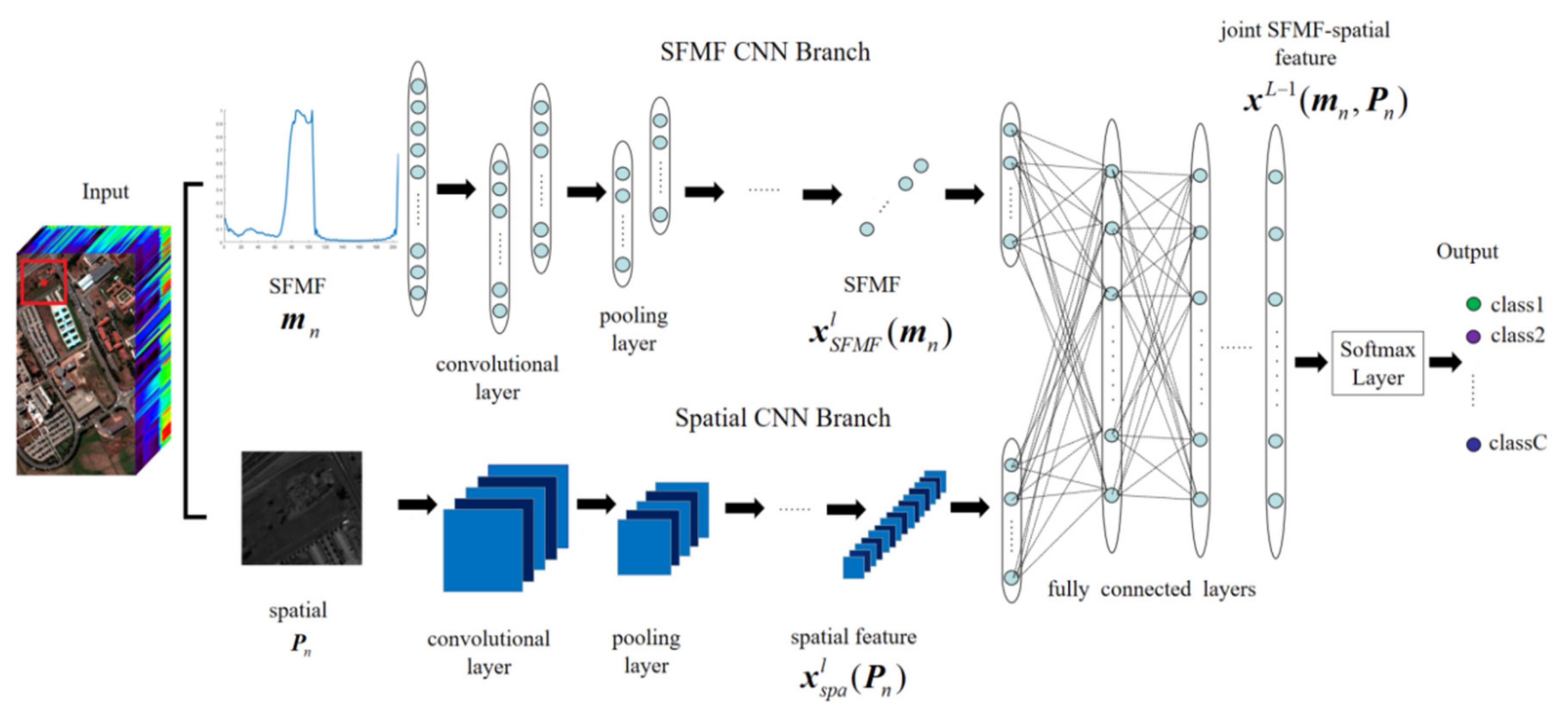
3.2.1. Proposed Two-Branch CNNs

We present two two-branch CNNs, i.e., Two-CNN_SFMF-spa and Two-CNN_fre-spe, to jointly learn the SFMF-spatial and frequency spectrum-spectral features, respectively. Shown in Figure 1 is the Two-CNN_SFMF-spa whose two branches are fed into the presented SFMF and spatial feature respectively, each branch has l convolution and pooling layers and L fully connected layers.

The SFMF of the n-th pixel is denoted as ${\mathit{m}}_n$. In the branch fed into the presented SFMF, the convolution and pooling layers are all 1-D, ${\mathit{x}}_{SFMF}^l({\mathit{m}}_n)$ is the output after the l layers’ convolution and pooling operations, which can be regarded as the results of further extracted SFMF. In the other branch fed into the spatial feature, to fuse the spatial information of all bands and suppress noise, the images on all spectral bands were averaged in the experiment, and then the neighborhood pixels of the n-th pixel, i.e., spatially adjacent patch $\mathit{P}(n)\in {\mathfrak{R}}^{r\times r}$ (r is the patch size, and in the experiment, the patch size is 21 × 21), is the input. The patch size is selected considering both the data structure and the network depth, under the condition of the same network depth, a smaller patch size will speed up the learning process while the recognition accuracy will decrease, or vice versa. The adjacent patch is a 2-dimensionality (2-D) information, so the convolution and pooling operations in this branch are all 2-D, and the output ${\mathit{x}}_{spa}^l({\mathit{P}}_n)$ can be regarded as the results of further extracted spatial feature.

To obtain the joint SFMF-spatial feature, ${\mathit{x}}_{SFMF}^l({\mathit{m}}_n)$ and ${\mathit{x}}_{spa}^l({\mathit{P}}_n)$ are mixed, i.e., are directly jointed, and fed into the first fully connected layer, the output of the first fully connected layer is

$${\mathit{x}}^1({\mathit{m}}_n,{\mathit{P}}_n)=g\{{\mathit{W}}^1·[{\mathit{x}}_{SFMF}^l({\mathit{m}}_n)\otimes {\mathit{x}}_{spa}^l({\mathit{P}}_n)]+{\mathit{b}}^1\}$$

(5)

where ${\mathit{W}}^1$ and ${\mathit{b}}^1$ are the weight matrix and bias of the first fully connected layer respectively, the output of the penultimate fully connected layer can be regarded as the extracted fusion deep SFMF-spatial feature, and the probability distribution of each category is predicted by inputting this feature into the softmax regression layer. The expression for the probability distribution is

$$\mathit{p}(n)=\frac{1}{{\displaystyle \sum _{k=1}^C{e}^{{\mathit{W}}_k^L{\mathit{x}}^{L-1}({\mathit{m}}_n,{\mathit{P}}_n)}}}\left[\begin{array}{c}{e}^{{\mathit{W}}_1^L{\mathit{x}}^{L-1}({\mathit{m}}_n,{\mathit{P}}_n)}\\ e^{{\mathit{W}}_2^L{\mathit{x}}^{L-1}({\mathit{m}}_n,{\mathit{P}}_n)}\\ ⋮\\ e^{{\mathit{W}}_C^L{\mathit{x}}^{L-1}({\mathit{m}}_n,{\mathit{P}}_n)}\end{array}\right]$$

(6)

where C is the number of categories and $\mathit{p}(n)$ is a vector with C elements, representing the probability that the n-th pixel belongs to each category. ${\mathit{W}}_k^L$ is the k-th row of the weight matrix of the softmax regression layer.

In the same way, we also construct the Two-CNN_fre-spe whose two branches are fed with the presented frequency spectrum feature ${\mathit{f}}_n$ and the spectral pixel feature ${\mathit{s}}_n$ respectively. After l layers 1-D convolution and pooling operations, two branches respectively output features ${\mathit{x}}_{fre}^l({\mathit{f}}_n)$ and ${\mathit{x}}_{spe}^l({\mathit{s}}_n)$ which are mixed and fed into the fully connected layers, and the output of the first fully connected layer is

$${\mathit{x}}^1({\mathit{f}}_n,{\mathit{s}}_n)=g\{{\mathit{W}}^1·[{\mathit{x}}_{fre}^l({\mathit{f}}_n)\otimes {\mathit{x}}_{spe}^l({\mathit{s}}_n)]+{\mathit{b}}^1\}$$

(7)

which is the fusion feature of the extracted deep frequency spectrum and spectral pixel features. Similarly, the classification of HRSIs can be completed after the softmax layer.

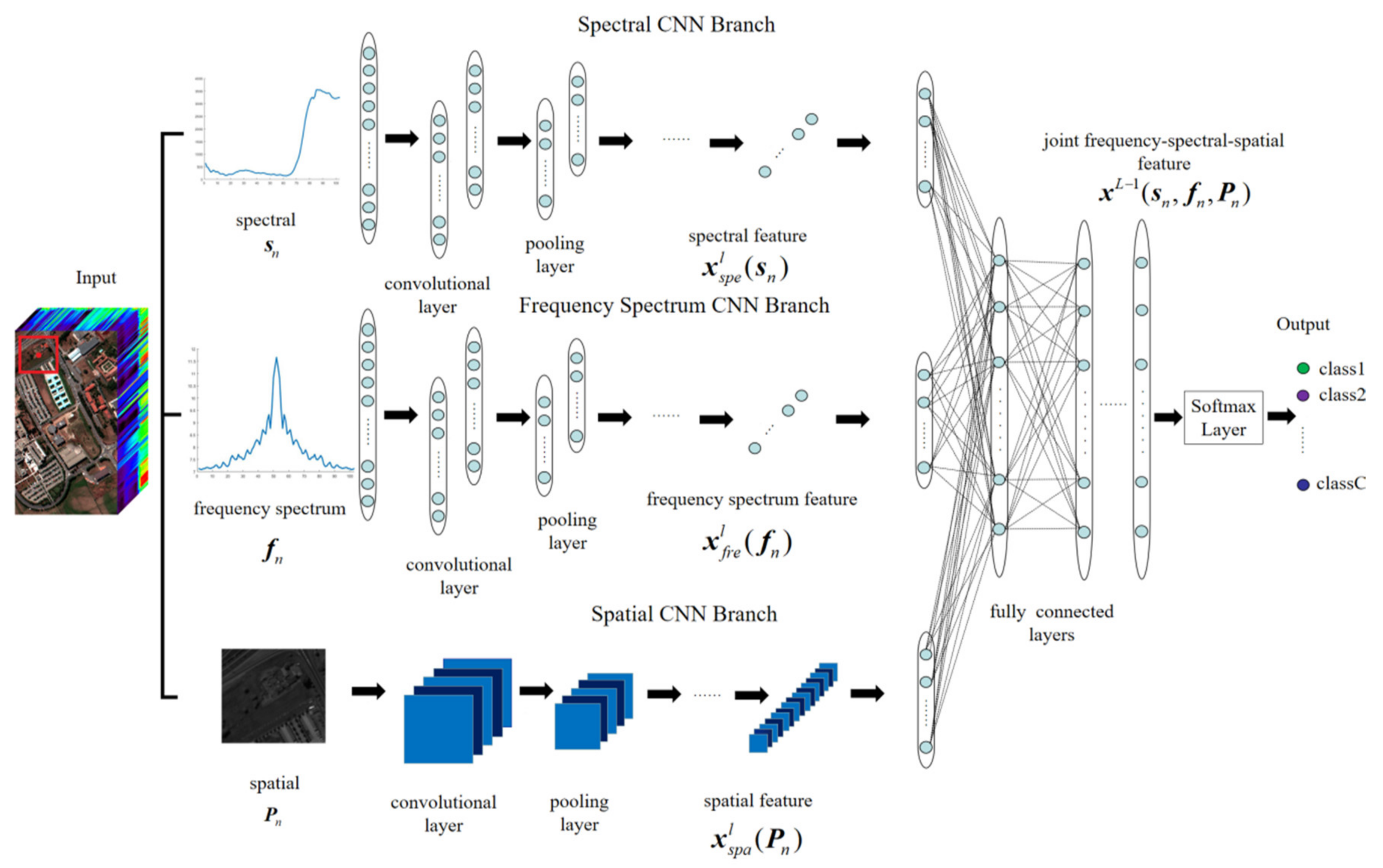
3.2.2. Proposed Three-Branch CNN

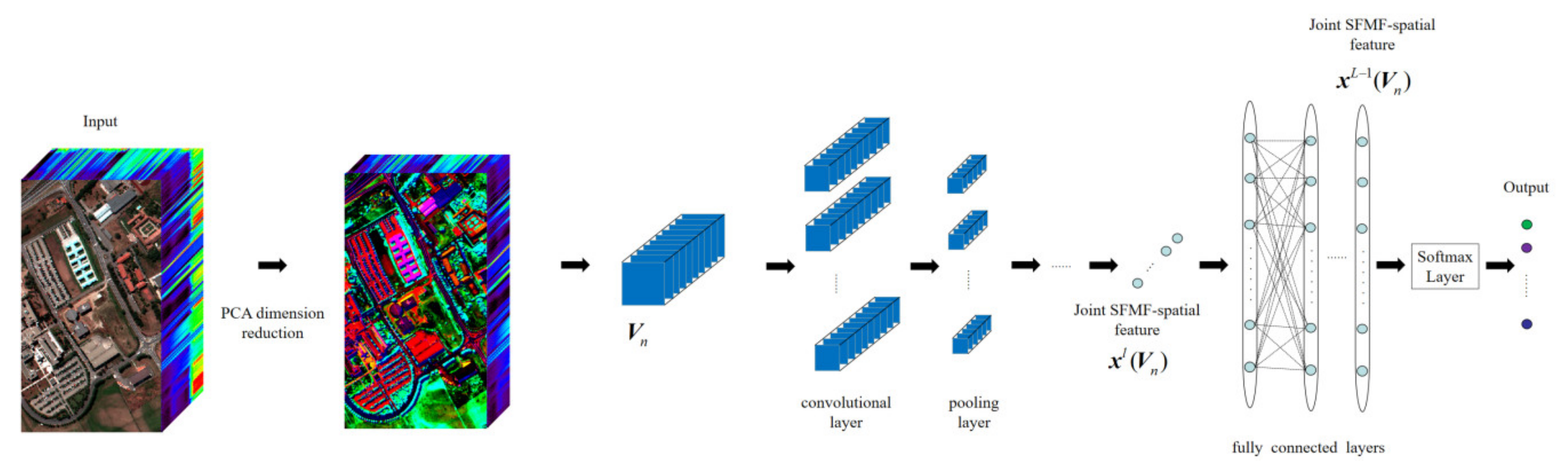
We present a three-branch CNN, i.e., Three-CNN, to jointly learn the spectral-frequency spectrum-spatial features, the detailed architecture is shown in Figure 2.

For the n-th pixel, the resulted outputs of the three branches are respectively denoted as ${\mathit{x}}_{spe}^l({\mathit{s}}_n)$, ${\mathit{x}}_{fre}^l({\mathit{f}}_n)$, and ${\mathit{x}}_{spa}^l({\mathit{P}}_n)$, which are the extracted deep spectral, frequency spectrum, and spatial features respectively. After mixing the resulted deep features of each branch by direct jointing them, we have spectral, frequency spectrum, and spatial mixed feature, and it is put into the fully connected layer for further feature extraction, and the output of the first fully connected layer is

$${\mathit{x}}^1({\mathit{s}}_n,{\mathit{f}}_n,{\mathit{P}}_n)=g\{{\mathit{W}}^1·[{\mathit{x}}_{spe}^l({\mathit{s}}_n)\otimes {\mathit{x}}_{fre}^l({\mathit{f}}_n)\otimes {\mathit{x}}_{spa}^l({\mathit{P}}_n)]+{\mathit{b}}^1\}$$

(8)

which is the fusion deep feature of the spectral, frequency spectrum, and spatial. The output of the penultimate fully connected layer can be regarded as the extracted fusion deep spectral-frequency spectrum-spatial feature. After the processing of the softmax regression layer, the probability distribution of each category can be obtained to complete the classification. The presented three-CNN comprehensively uses spectral, frequency spectrum, and spatial features, and the resulted deep fusion feature conceives much more nonlinear discriminant information than those resulting from the CNNs fed with not all of the three original features.

3.3. 3-D CNN-PCA

An HRSI is a joint spectral-spatial image, its data have a 3-D structure that contains spatial continuity information and spectral continuity information of the targets. The traditional 2-D CNN can extract the spatial features of HRSIs but does not make full use of the spectral feature. A 3-D CNN-PCA model is presented to extract the joint SFMF-spatial feature, 3-D CNN-PCA firstly uses PCA to perform dimensionality reduction along the SFMF, and then sends the reduced SFMF-spatial cube to a 3-D CNN for further deep feature extraction and classification. PCA is used to reduce information redundancy while reducing computational complexity.

In this paper, the structure of the presented 3-D CNN-PCA model that extracts the joint SFMF-spatial feature is shown in Figure 3.

After the dimensionality reduction by PCA, the pixel cube composed of the reduced SFMF features of the n-th pixel and its adjacent pixels, i.e., $\mathit{V}(n)\in {\mathfrak{R}}^{h\times w\times l}$ (h, w, l are the height, width, and length of the cube respectively) is used as the input of the 3-D CNN. For the n-th pixel, the resulted outputs obtained after 3-D convolution operation and pooling operation is ${\mathit{x}}^l({\mathit{V}}_n)$, which is the extracted deep joint SFMF-spatial feature, and it is put into the fully connected layer for further feature extraction, and the output of the first fully connected layer is

$${\mathit{x}}^1({\mathit{V}}_n)=g[{\mathit{W}}^1·{\mathit{x}}_{}^l({\mathit{V}}_n)+{\mathit{b}}^1]$$

(9)

which is a deeper feature of extracted joint SFMF-spatial feature. After the softmax layer, the terrain classification is completed.

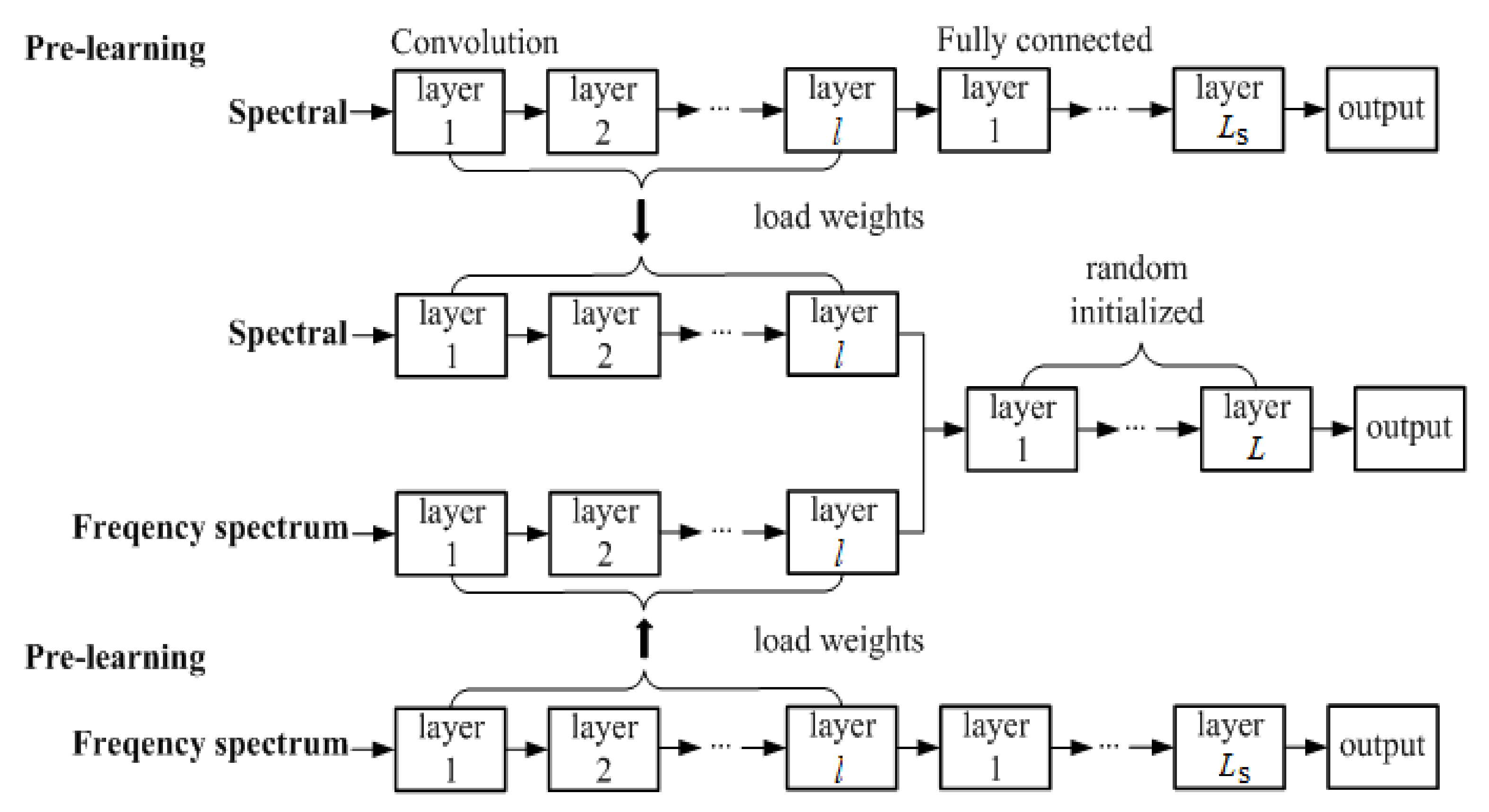
3.4. Proposed Pre-Learning Strategy

A pre-learning strategy is proposed for training the presented multi-branch CNNs. All convolution kernels and biases in a CNN need to be trained with the training data $\left\{{\mathit{m}}_n,{\mathit{s}}_n,{\mathit{f}}_n,{\mathit{P}}_n,c(n)\right\}$,$n=0,1,\dots ,N$. The loss function of the softmax regression layer is

$$J(\theta )=-\frac{1}{N}{\displaystyle \sum _{n=1}^N{\displaystyle \sum _{k=1}^{C}1\{k=c(n)\}\log p_k(n)}}$$

(10)

where N is the number of training samples; $c(n)$ is the class label of the n-th training sample; $p_k(n)$ is the k-th element of $\mathit{p}(n)$ which is the probability that the n-th pixel is assigned to the k-th class; $1\{·\}$ is an indicative function, the result is 1 if the conditions in parentheses are met, otherwise, it is 0. $\theta$ represents the set of convolution kernels, weight matrices, and the bias values to be trained.

The common methods of CNN weight initialization include Gaussian distribution initialization, Uniform distribution initialization, and Xavier initialization [27]. However, the above initialization methods are all random initialization methods that meet certain rules, which have no pertinence to the input data and need a long time to train and adjust the parameters.

The presented pre-learning strategy is: using the same training data to train a basic single-branch CNN, and then the low-level weights, the values of the convolution kernels, and the biases of the convolution layers are all taken as the initialization values of the corresponding branch in a multi-branch CNN. Shown in Figure 4 is a Two-CNN training schematic diagram with the spectral pixel and frequency spectrum as inputs.

As shown in Figure 4, the sizes of the convolution kernels, convolution layers, and pooling layers in the two-branch network are the same as the sizes of those in each single-branch network; $L\mathrm{s}$ is the number of the fully connected layers in each single-branch CNN. The weights and biases values of the trained spectral and the frequency spectrum single-branch CNNs are used to initialize the two-branch CNN. The initialization values get by the pre-learning method are more targeted to the input data, which can speed up the convergence rate of the multi-branch network and prevent the network from falling into a locally optimal solution to a certain extent.

4. Experiment Results

Using same training samples and testing samples, the experimental results of the basic CNN fed with frequency spectrum feature (CNN_fre), the experimental results of the basic CNN fed with spectral feature (CNN_spe), basic CNN fed with the presented SFMF (CNN_SFMF), presented Two-CNN_fre-spe, presented Two-CNN_SFMF-spa, Two-CNN fed with spectral and spatial features (Two-CNN_spe-spa), presented 3-D CNN-PCA fed with the HRSIs containing SFMF feature (3-D CNN-PCA_SFMF-spa), and 3-D CNN and PCA combination method fed with the original HRSI (3-D CNN-PCA_spe-spa) are compared.

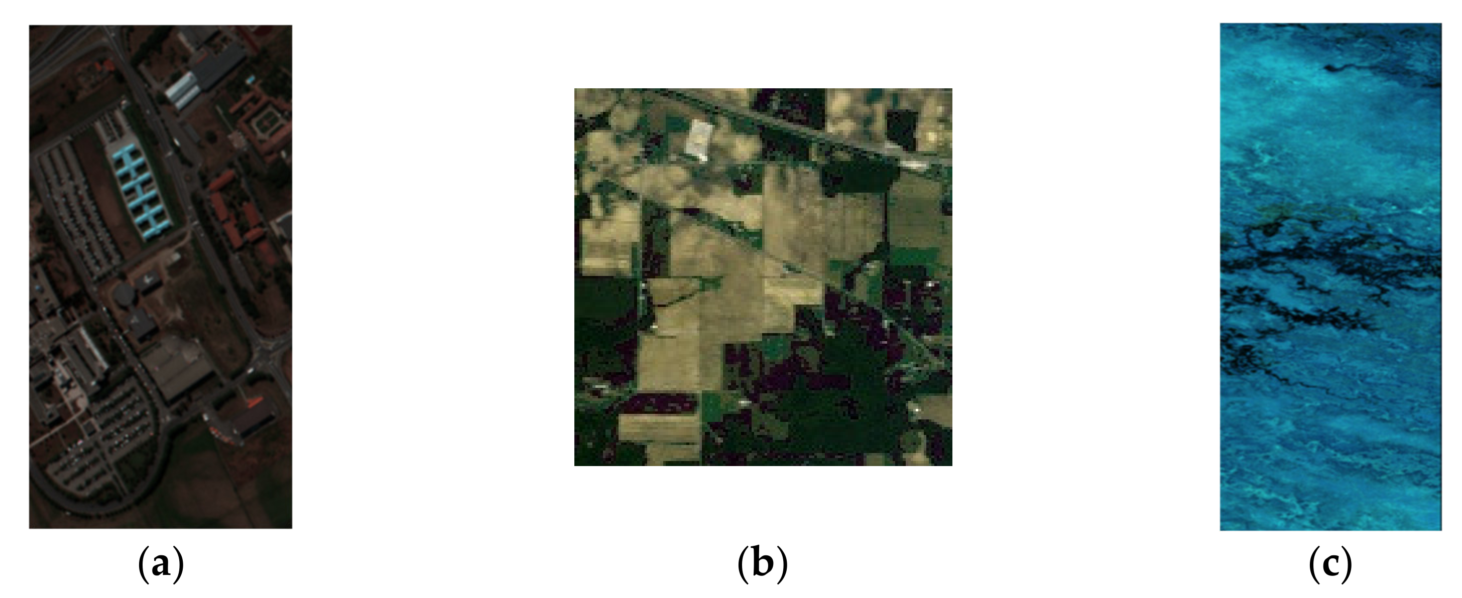
4.1. Experiment Datasets

In this paper, three real HRSIs were used for the experiments, namely Pavia University, Indian Pines, and Botswana. Shown in Figure 5 are the RGB false-color images of the three HRSIs.

Pavia University HRSI was imaged by a reflective optics system imaging spectrometer (ROSIS) in Pavia City, Italy in 2003. After eliminating the noise and water absorption bands, 103 spectral bands were retained. It has 9 ground objects, with a total data size of 610 × 340.

Indian Pines HRSI was taken in 1992 in Indiana by the airborne visible/infrared imaging spectrometer (AVIRIS). It has 220 spectral bands and contains 16 kinds of terrain, the image size is 145 × 145.

Botswana HRSI was acquired by NASA EO-1 satellite in Okavango Delta, Botswana on 31 May 2001. After eliminating the water absorption and noise bands, 145 bands were retained.

4.2. CNNs Structure Design and Parameter Setting

The structure and parameter settings of CNNs have an important impact on the final results, but it is difficult to determine them theoretically. The complexity of network structure has a lower limit, that is, its complexity must exceed the complexity of the problem. Based on ensuring sufficient complexity, the network structure should make the data information flow efficiently in the network. For adequately dimensioning the minimum number l of convolution and pooling layers and the number L of fully connected layers, we design the lower limit of network structure through the interpretation of data information structure, hence the hierarchy in the results changes with the data sets.

Table 1. Architecture of basic CNN and 3-D CNN on each dataset.

Layer Name			I1	C2 S3	C4 S5	C6 S7	C8 S9	C10 S11	F12	F13	O14
Kernel Size	Pavia	Spectral/ SFMF	1 × 103/ 1 × 206	1 × 8 1 × 2	1 × 7 1 × 2	1 × 8 1 × 2	-	-	F	F	1 × 9
		Spatial	21 × 21	3 × 3 2 × 2	3 × 3 2 × 2	-	-	-			1 × 9
		Fre. spectrum	1 × 103	1 × 103	-	-	-	-			1 × 9
		SFMF-Spa.	21 × 21 × 80	3 × 3 × 3 2 × 2 × 2	3 × 3 × 3 2 × 2 × 2	-	-	-			1 × 9
		Spectral-Spa.	21 × 21 × 40	3 × 3 × 3 2 × 2 × 2	3 × 3 × 3 2 × 2 × 2	-	-	-			1 × 9
	Indian	Spectral/ SFMF	1 × 220/ 1 × 440	1 × 5 1 × 2	1 × 5 1 × 2	1 × 4 1 × 2	1 × 5 1 × 2	1 × 4 1 × 2			1 × 16
		Spatial	21 × 21	3 × 3 2 × 2	3 × 3 2 × 2	-	-	-			1 × 16
		Fre. spectrum	1 × 220	1 × 220	-	-	-	-			1 × 16
		SFMF-Spa.	21 × 21 × 175	3 × 3 × 3 2 × 2 × 2	3 × 3 × 3 2 × 2 × 2	-	-	-			1 × 16
		Spectral-Spa.	21 × 21 × 100	3 × 3 × 3 2 × 2 × 2	3 × 3 × 3 2 × 2 × 2	-	-	-			1 × 16
	Bot	Spectral/ SFMF	1 × 145/ 1 × 290	1 × 8 1 × 2	1 × 7 1 × 2	1 × 8 1 × 2	-	-			1 × 14
		Spatial	21 × 21	3 × 3 2 × 2	3 × 3 2 × 2	-	-	-			1 × 14
		Fre. spectrum	1 × 145	1 × 145	-	-	-	-			1 × 14
		SFMF-Spa.	21 × 21 × 30	3 × 3 × 3 2 × 2 × 2	3 × 3 × 3 2 × 2 × 2	-	-	-			1 × 14
		Spectral-Spa.	21 × 21 × 90	3 × 3 × 3 2 × 2 × 2	3 × 3 × 3 2 × 2 × 2	-	-	-			1 × 14
FeatureMap	Pavia	Spectral/ SFMF	1	6	12	24	-	-	256	-	9
		Spatial	1	30	30	-	-	-	400	400	9
		Fre. spectrum	1	103	-	-	-	-	256	-	9
		SFMF-Spa.	1	6	12	-	-	-	256	-	9
		Spectral-Spa.	1	6	12	-	-	-	256	-	9
	Indian	Spectral/ SFMF	1	6	12	24	48	96	256	-	16
		Spatial	1	30	30	-	-	-	256	256	16
		Fre. spectrum	1	220	-	-	-	-	256	-	16
		SFMF-Spa.	1	6	12	-	-	-	256	-	16
		Spectral-Spa.	1	6	12	-	-	-	256	-	16
	Bot	Spectral/ SFMF	1	6	12	24	-	-	256	-	14
		Spatial	1	6	12	-	-	-	256	-	14
		Fre. spectrum	1	145	-	-	-	-	256	-	14
		SFMF-Spa.	1	6	12	-	-	-	256	-	14
		Spectral-Spa.	1	6	12	-	-	-	256	-	14

shows the architectures of the CNNs for the three data sets, “Pavia”, “Indian”, “Bot”, “Freq.”, and “Spa.” are the abbreviations of “Pavia University”, “Indian Pines”, “Botswana”, “Frequency”, and “Spatial” respectively. I, C, S, F, and O represent the input layer, convolution layers, pooling layers, fully connected layers, and output layer, respectively. For example, C2 is the convolution layer which is the second layer in the whole neural network. In this paper, the convolution kernel and weight initializations of the basic CNNs use the Glorot uniform method, the bias is initialized to 0, the learning rate in the optimization algorithm Adam [28] is set to 0.001, and the batch size in the experiments is 5.

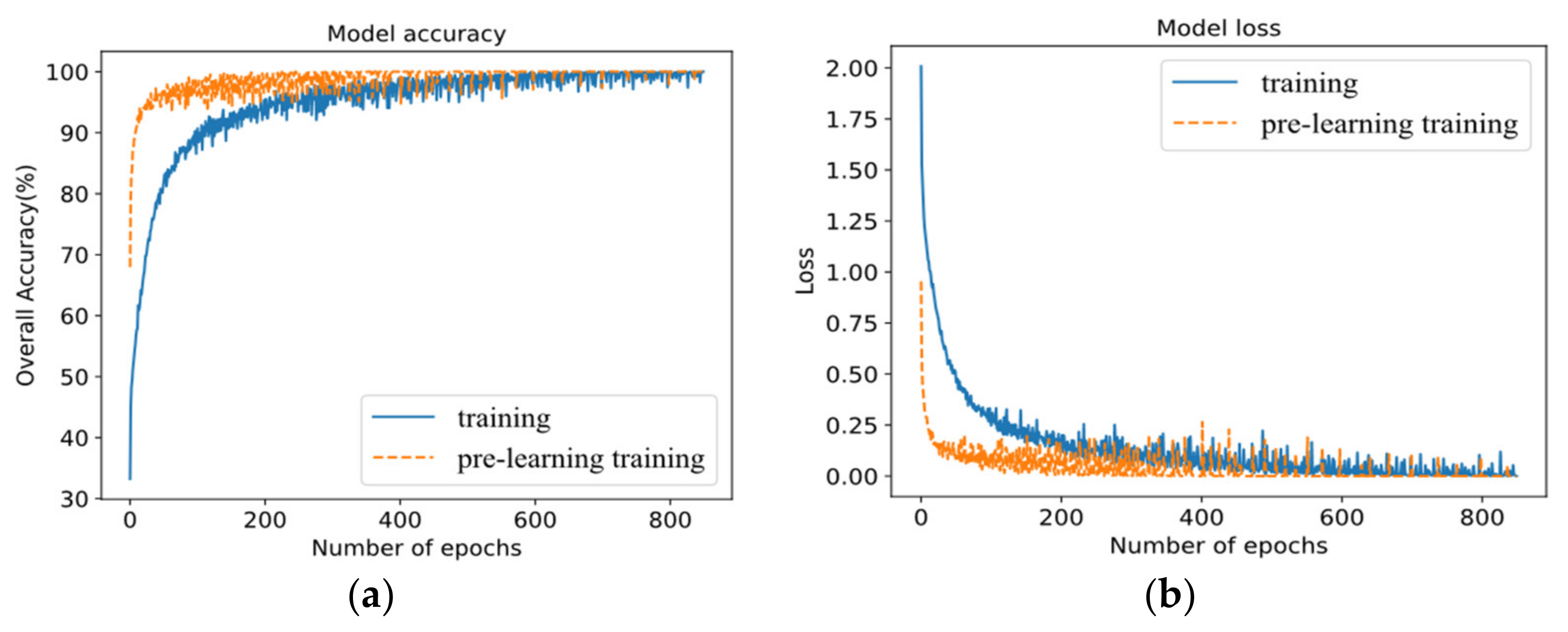
4.3. Effectiveness Analysis of Proposed Pre-Learning Training Strategy

To verify the effectiveness of the proposed pre-learning training strategy, 20% labeled samples of Indian Pines image are randomly selected as training data, under the condition of the same training data, the convergence speed of the overall accuracy, and the loss of the two-branch CNN model using the presented pre-learning training strategy are compared with those of the same two-branch CNN model not using the pre-learning training strategy. Figure 6 shows the comparison of different training strategies on Two-CNNfre-spe.

Figure 6 shows that the two-branch CNN using the presented pre-learning training strategy converges faster during training, which proves that the pre-learning training strategy can effectively accelerate the convergence speed of network training and prevent the network from falling into the local optimal solution to a certain extent.

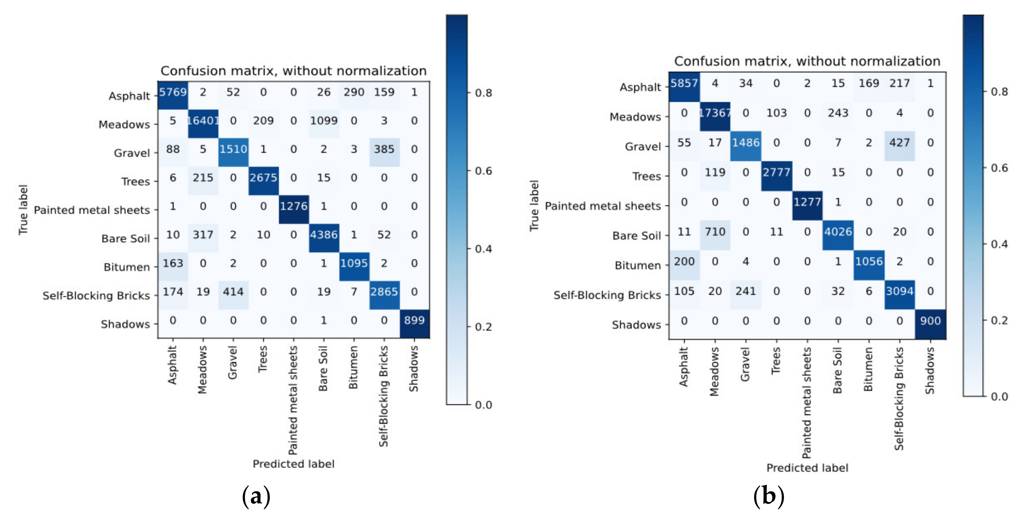
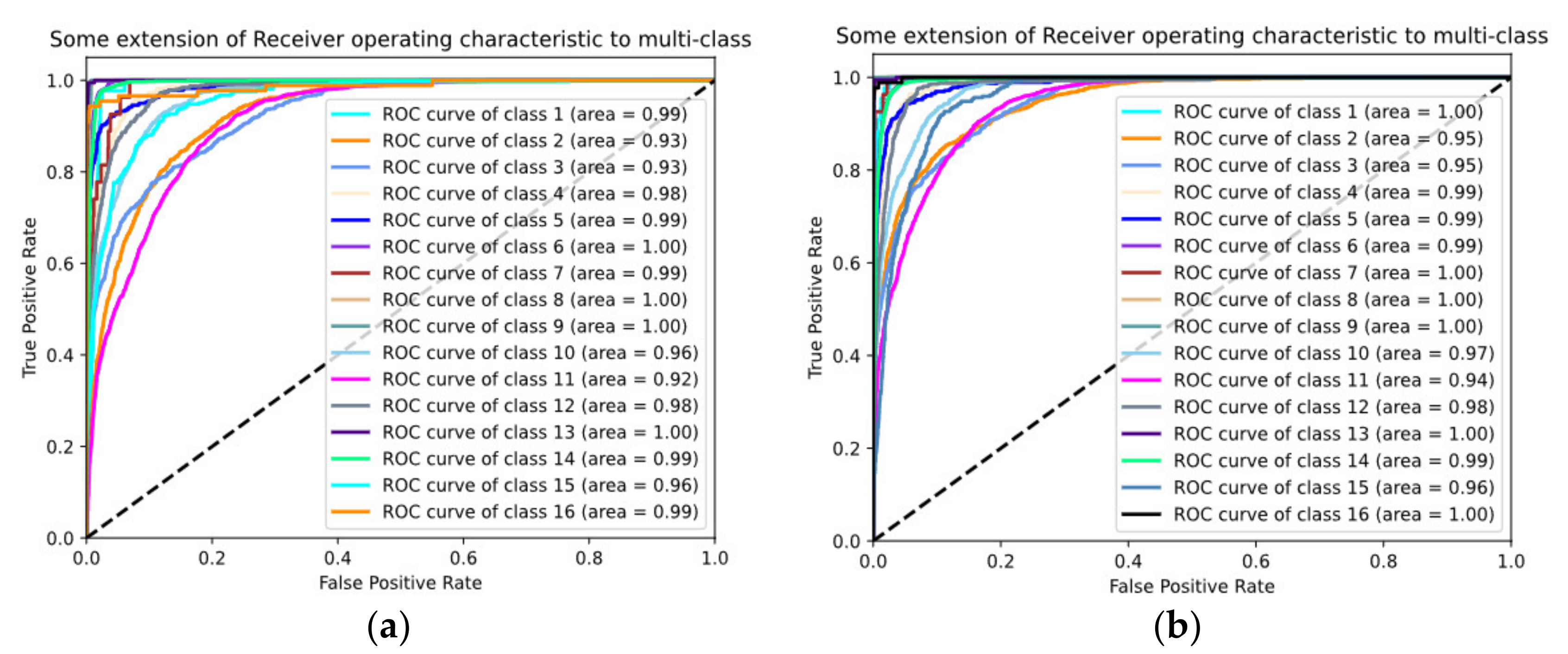
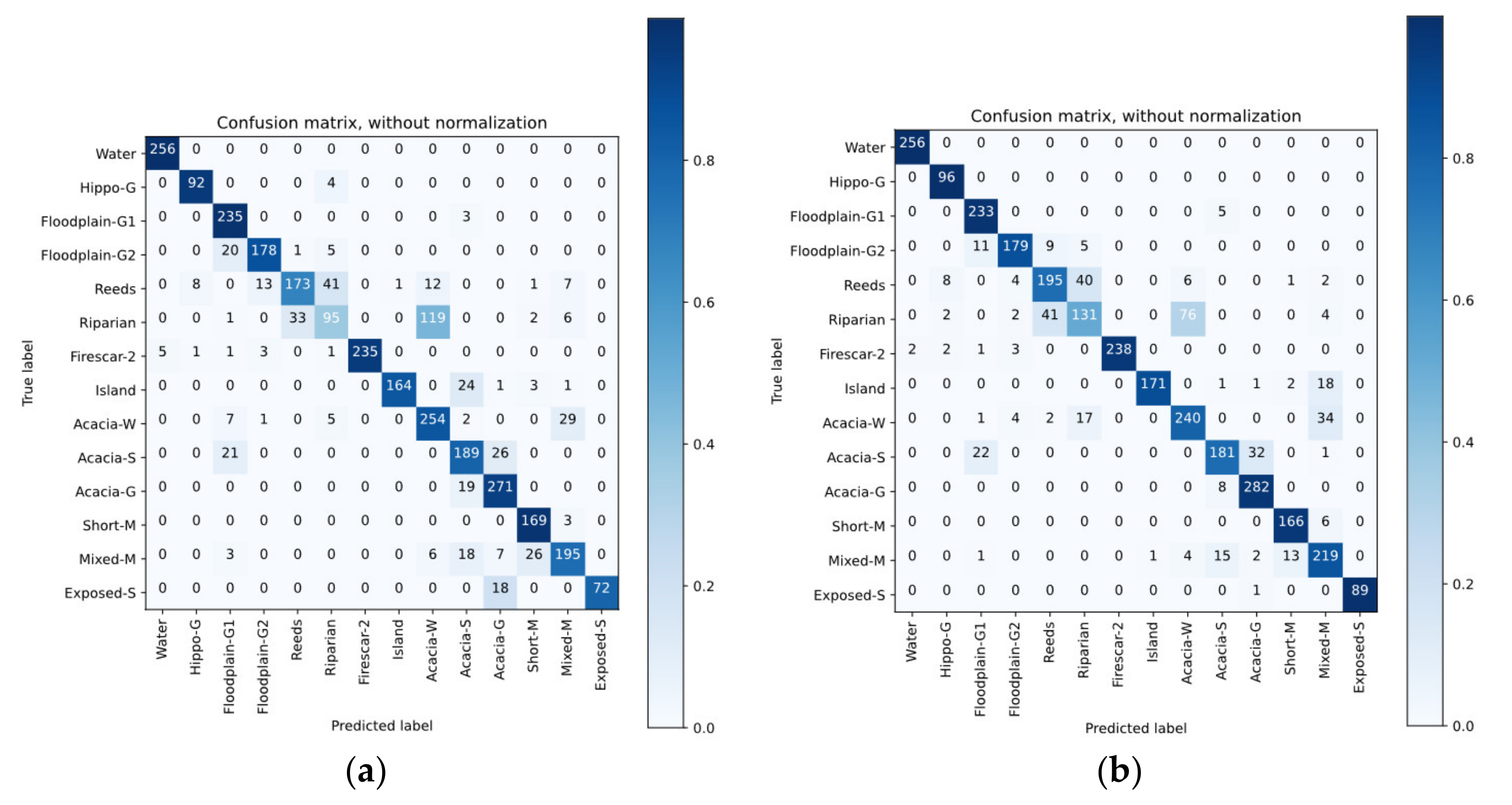
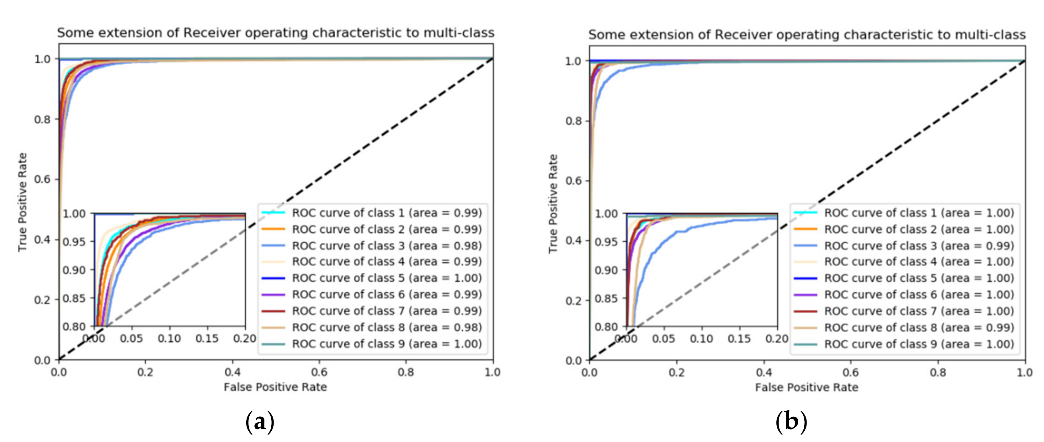
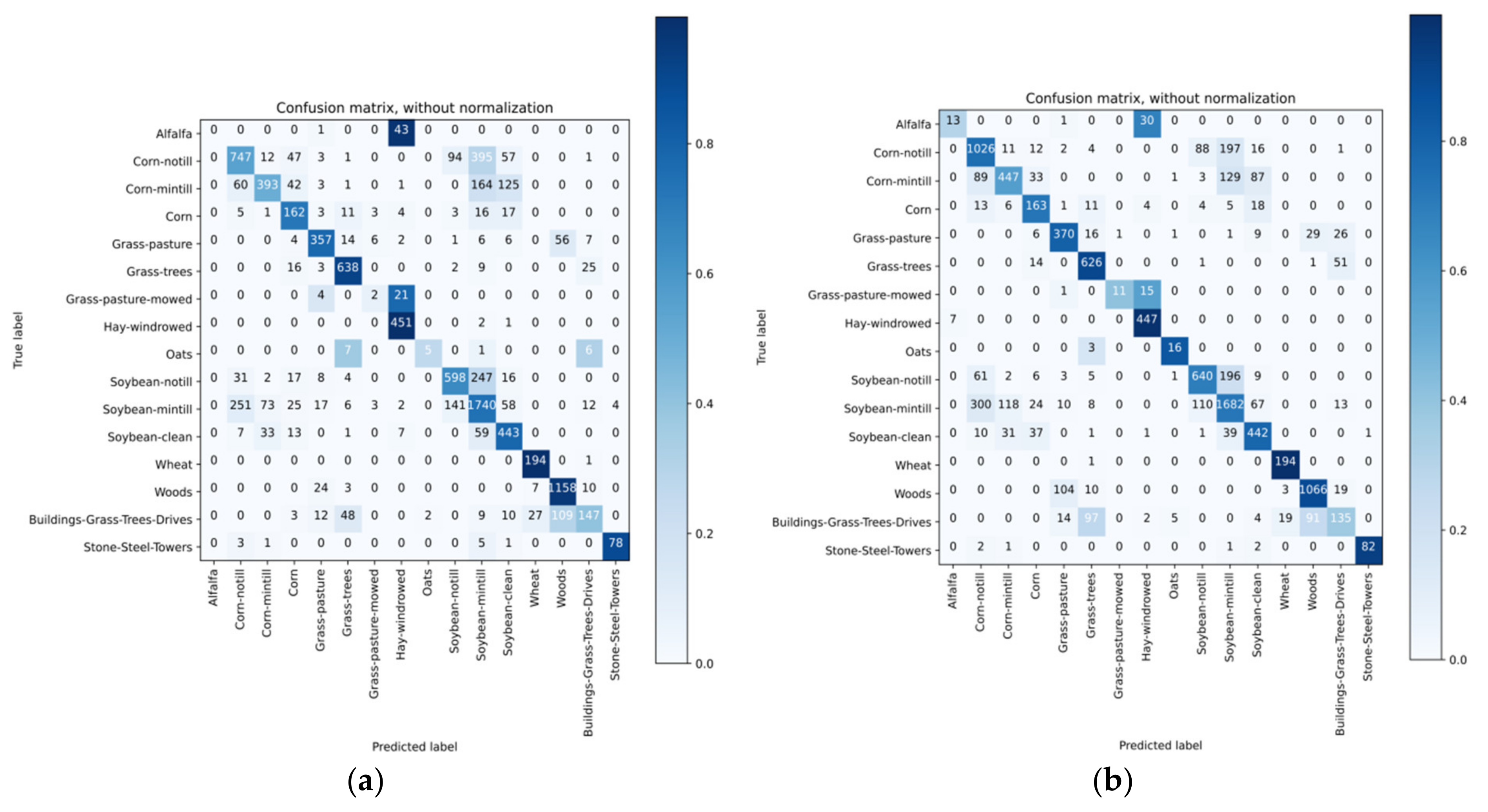
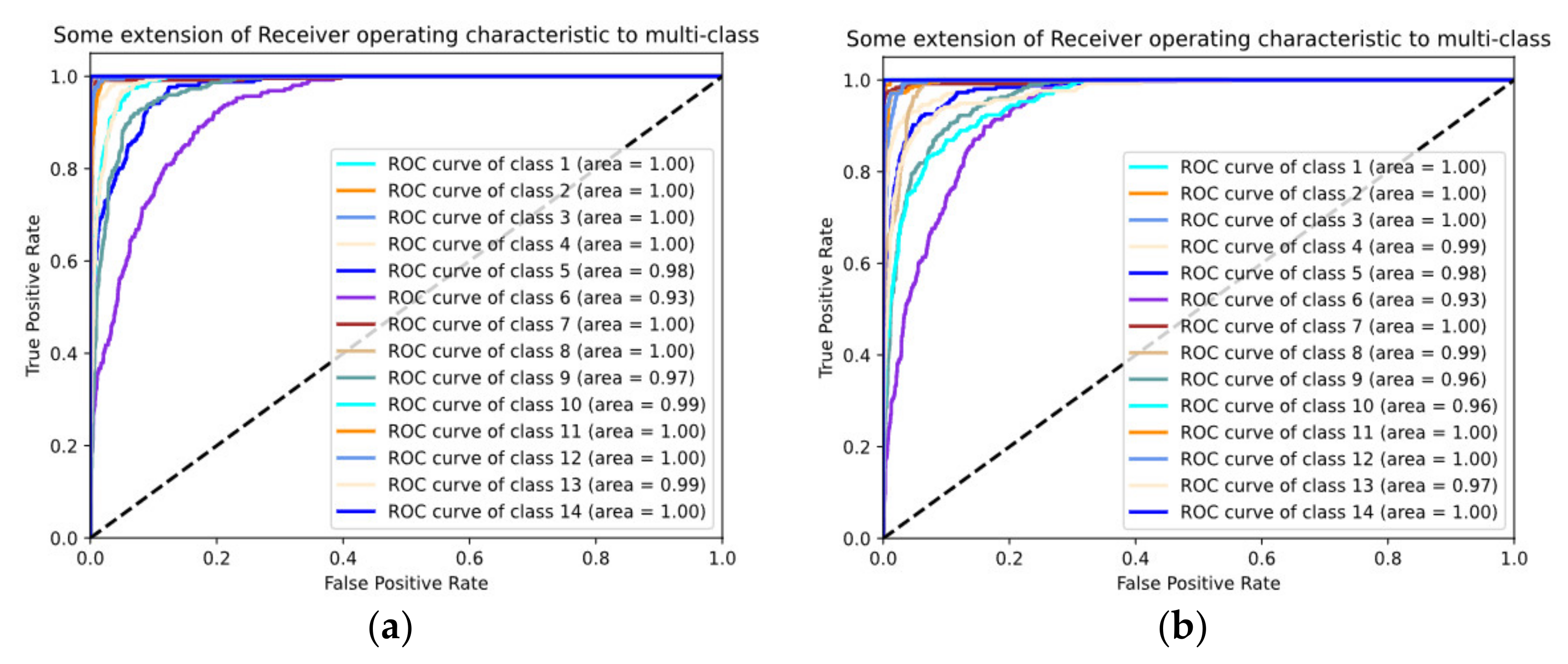
4.4. Classification Results

In the experiments, for each HRSI, 5%, 10%, and 20% of the labeled samples of each class are randomly selected as the training samples, and the rest are testing samples. The average overall accuracy (AOA) of ten runs and the standard deviation (SD), confuse matrix, and receiver operating characteristic (ROC) curve are used to evaluate the performance of the network. AOA is the average of the ratio of the number of correctly recognized samples to that of all samples, and the computational cost of each model is given, "M" represents a million operations. All programs in the experiment were implemented in Python, and the CNN models were constructed using the Tensorflow-based deep learning framework Keras. All multi-branch CNNs are trained by the presented pre-learning training strategy. The optimal recognition result of each column is shown in boldface.

It can be seen from

Table 2. Classification results of Pavia University image.

Ratio of Training Samples	5%	10%	20%	Computational Cost
	AOA(%) ± SD(%)	AOA(%) ± SD(%)	AOA(%) ± SD(%)
CNNfre	89.62 ± 0.42	91.73 ± 0.34	92.41 ± 0.29	2.19 M
CNNspe	91.32 ± 1.32	93.06 ± 0.61	93.98 ± 0.50	5.74 M
CNNSFMF	92.83 ± 0.70	94.07 ± 0.36	94.65 ± 0.36	22.32 M
Two-CNNfre-spe	93.65 ± 0.03	94.99 ± 0.03	95.74 ± 0.03	21.39 M
Two-CNNspe-spa	93.24 ± 0.30	96.36 ± 0.71	98.54 ± 0.34	111.44 M
Two-CNNSFMF-spa	93.41 ± 0.13	96.73 ± 0.20	98.67 ± 0.05	228.41 M
Three-CNN	93.39 ± 0.16	96.62 ± 0.18	98.55 ± 0.22	122.63 M
3-D CNN-PCAspe-spa	98.37 ± 0.20	98.74 ± 1.13	99.77 ± 0.06	910.15 M
3-D CNN-PCASFMF-spa	98.51 ± 0.20	99.12 ± 0.14	99.78 ± 0.05	3695.57 M

that under 5%, 10%, and 20% training data, the AOAs of CNN_fre are 1.7%, 1.33%, and 1.57% lower than those of CNN_spe, which shows that the sole frequency spectrum feature is not better than the sole spectral feature; the AOA is increased 1.51, 1.01, and 0.67 percentage points by CNN_SFMF respectively compared with CNN_spe; the AOA is increased by 2.33, 1.93 and 1.76 percentage points by Two-CNN_fre-spe respectively compared with CNN_spe; the AOA is increased by 0.14, 0.38, and 0.01 percentage points by 3-D CNN-PCA_SFMF-spa respectively compared with 3-D CNN-PCA_spe-spa. Multi-branch CNNs fully use different features, and finally can obtain fusion deep features. By comparing the multi-branch CNNs fed with the spatial feature and 3-D CNN-PCA_spe-spa, it is found that introducing the frequency spectrum feature can also obtain better classification accuracy. Comparing the SDs of the experimental results, we can see that the SDs of the experimental results obtained by the methods adding the presented frequency spectrum feature are smaller, indicating that the classification results of the methods adding the frequency spectrum feature are more stable. By comparing the computational cost of each model, it can be concluded that the addition of frequency spectrum features can improve the classification efficiency of the model and slightly increase the calculational cost of the model.

Figure 7 and Figure 8 are the confusion matrixes and ROC curves of the CNN_spe and CNN_SFMF methods under 5% training data of the Pavia University dataset. The diagonal value in the confusion matrix represents the number of pixels correctly classified in the testing data. Figure 7 shows that there are 964 more diagonal pixels in the confusion matrix of CNN_SFMF which uses the presented spectral and frequency spectrum mixed feature than those in the confusion matrix of CNN_spe which only uses the spectral feature. The area under the ROC curve can be used to indicate the classification efficiency of the model. The larger the area, the better the classification efficiency. Figure 8 shows that the area of the ROC curve of each class of CNN_SFMF is larger than that of CNN_spe.

According to

Table 3. Classification results of Indian Pines image.

Ratio of Training Samples	5%	10%	20%	Computational Cost
	AOA(%) ± SD(%)	AOA(%) ± SD(%)	AOA(%) ± SD(%)
CNNfre	63.39 ± 0.21	70.31 ± 0.39	76.84 ± 0.57	21.30 M
CNNspe	74.44 ± 1.28	81.22 ± 2.30	85.75 ± 1.46	18.44 M
CNNSFMF	77.06 ± 1.64	83.15 ± 1.36	86.11 ± 0.82	68.71 M
Two-CNNfre-spe	78.28 ± 0.24	83.42 ± 0.22	87.56 ± 0.31	125.48 M
Two-CNNspe-spa	64.50 ± 1.16	85.91 ± 0.33	95.52 ± 0.35	238.18 M
Two-CNNSFMF-spa	68.25 ± 0.20	87.87 ± 0.74	95.55 ± 0.29	502.88 M
Three-CNN	64.77 ± 1.19	86.01 ± 0.85	95.63 ± 0.14	345.22 M
3-D CNN-PCAspe-spa	93.16 ± 0.42	97.37 ± 0.11	99.00 ± 0.17	5790.30 M
3-D CNN-PCASFMF-spa	94.67 ± 0.42	97.63 ± 0.25	99.07 ± 0.16	17,811.00 M

under 5%, 10%, and 20% training data, the AOAs of CNN_fre are 11.05, 10.91, and 8.91 percentage points lower than those of CNN_spe; the AOAs of CNN_SFMF are 2.62, 1.93, and 0.36 percentage points higher than those of CNN_spe; the AOAs of Two-CNN_fre-spe are 3.84, 2.20, and 1.81 percentage points higher than those of CNN_spe; the AOAs of 3D-CNN-PCA_SFMF-spa are 1.51, 0.26, and 0.07 percentage points higher than those of 3-D CNN-PCA_spe-spa. By comparing with the multi-branch CNNs fed with the spatial feature, it is found that introducing the frequency spectrum feature obtains better classification accuracy.

Figure 9 and Figure 10 are the confusion matrixes and ROC curves of the CNN_spe and CNN_SFMF methods under the 5% training data of the Indian Pines dataset. Figure 9 shows that the confusion matrix of CNN_SFMF has 247 more diagonal pixels than the confusion matrix of CNN_spe. Figure 10 shows that the area of the ROC curve of each class of CNN_SFMF is larger than that of CNN_spe.

According to

Table 4. Classification results of Botswana image.

Ratio of Training Samples	5%	10%	20%	Computational Cost
	AOA(%) ± SD(%)	AOA(%) ± SD(%)	AOA(%) ± SD(%)
CNNfre	83.19 ± 0.29	89.09 ± 0.71	91.93 ± 0.17	6.10 M
CNNspe	85.88 ± 1.47	89.39 ± 1.28	93.35 ± 0.62	11.28 M
CNNSFMF	87.08 ± 0.41	91.37 ± 0.47	93.74 ± 0.75	43.40 M
Two-CNNfre-spe	86.98 ± 0.29	91.43 ± 0.47	94.63 ± 0.26	42.14 M
Two-CNNspe-spa	63.84 ± 0.71	84.59 ± 0.62	91.50 ± 0.37	40.21 M
Two-CNNSFMF-spa	65.07 ± 0.75	84.87 ± 1.07	92.21 ± 0.29	100.59 M
Three-CNN	72.47 ± 1.42	85.17 ± 0.70	93.19 ± 0.28	71.06 M
3-D CNN-PCAspe-spa	90.84 ± 0.87	98.15 ± 0.48	99.68 ± 0.20	4684.49 M
3-D CNN-PCASFMF-spa	93.41 ± 0.87	98.63 ± 0.44	99.70 ± 0.11	506.36 M

under 5%, 10%, and 20% training data, the AOAs of CNN_fre are respectively 2.69%, 0.3%, and 1.42% less than those of CNN_spe; the AOAs of CNN_SFMF are respectively 1.20%, 1.98%, and 0.39% better than those of CNN_spe; the AOAs of Two-CNN_fre-spe are respectively 1.10%, 2.04%, and 1.28% better than those of CNN_spe; the AOAs of 3-D CNN-PCA_SFMF-spa are respectively 2.57%, 0.48%, and 0.02% better than those of 3-D CNN-PCA_spe-spa. By comparing with the multi-branch CNNs fed with the spatial feature and 3-D CNN-PCA, it is found that introducing the frequency spectrum feature obtains better classification accuracy. We can see that the SDs of the experimental results of the methods adding the frequency spectrum feature are smaller than those of the other methods. It also can be seen that the addition of the frequency spectrum feature can improve the classification efficiency and slightly increase the computational cost.

Figure 11 and Figure 12 are the confusion matrixes and ROC curves of the CNN_spe and CNN_SFMF methods under the 5% training data of the Botswana dataset. Figure 11 shows that there are 98 more diagonal pixels in the confusion matrix of CNN_SFMF than those in the confusion matrix of CNN_spe. Figure 12 shows that the area of the ROC curve of each class of CNN_SFMF is also larger than that of CNN_spe.

4.5. Discussion of Classification Results

From the above experimental results, it can be concluded that the addition of the frequency spectrum feature can effectively improve the classification accuracy of HRSIs. The addition of the frequency dimension would not bring with other classifiers including those based on more complex CNN architecture, because with the addition of dimension the discriminant information is also added, such that the classification accuracy will be improved using the classifiers with the same complexity. Compared with the other two datasets, the Indian Pines dataset has the most obvious improvement in classification accuracy, followed by the Pavia University dataset, and the Botswana dataset has a relatively small improvement in classification accuracy. Taking CNN_spe and Two-CNN_fre-spe as examples, under 5%, 10% and 20% of the training samples, the classification accuracy of Two-CNN_fre-spe is 2.62%, 2.00%, and 1.47% higher than that of CNN_spe on average for the Indian Pines dataset, Pavia University dataset, and Botswana dataset, respectively. From the classification accuracies of different datasets under 5%, 10%, and 20% training data, it can be concluded that the addition of the frequency spectrum feature in the case of fewer training samples can generally improve the classification accuracy. However, compared with the other two datasets, the number of labeled samples in Botswana is too small, although the addition of the frequency spectrum feature increases the classification information, it also leads to some overfitting, which leads to a relatively small improvement in classification accuracy.

The experimental results show that adding the presented frequency spectrum feature into CNNs can bring more separability information and obtain better classification accuracy, and the classification results are usually more stable. The presented multi-branch CNNs, i.e., Two-CNN_SFMF-spa, Two-CNN_fre-spe, and Three-CNN, based on pre-learning training strategy also get better classification results, this is because these multi-branch CNNs can extract more discriminative deep fusion features by employing several single branches of convolution and pooling layers. Compared with the ordinary CNNs methods using spectral pixel and spatial features, Two-CNN_SFMF-spa and Three-CNN employ the spectral pixel, pixel frequency spectrum, and spatial features to get the deep fusion features with more discriminative information.

The intrinsic reason behinds this is that the improvement of classification rate is achieved at the cost of a certain complexity in the architecture that follows the feature extraction. The addition of the frequency spectrum feature into CNNs comprises two steps, i.e., the classical shallow feature extraction and deep feature extraction. The frequency spectrum feature can be taken as the product of feature extraction by classical shallow learning. The presented SFMF feature is more complicated than the original spectral pixel feature because it combines spectral pixel and frequency spectrum features. When the frequency spectrum feature or the SFMF feature is imported to CNNs, the learning mechanism of CNNs naturally results in the corresponding deep feature, which is the outcome of deep learning.

5. Conclusions

In this paper, a deep feature extraction method for HRSIs based on mixed features and CNNs is proposed. The pixel frequency spectrum feature is presented and a mixed feature, i.e., SFMF is also presented. Several multi-branch CNNs fed with pixel frequency spectrum, SFMF, spectral pixel, and spatial features are also presented with a presented pre-learning training strategy, and a 3-D CNN-PCA_SFMF-spa method is presented to verify the effectiveness of introducing frequency spectrum feature. The experimental results on three real HRSIs show that adding frequency spectrum feature into CNN can effectively improve the classification accuracy and the presented multi-branch CNNs and 3-D CNN-PCA_SFMF-spa can extract more discriminative deep fusion features of HRSIs.

References

1. Tong, Q.; Xue, Y.; Zhang, L. Progress in Hyperspectral Remote Sensing Science and Technology in China over the Past Three Decades. IEEE J. Sel. Top. Appl. Earth Obs. Remote Sens. 2014, 7, 70–91. [Google Scholar] [CrossRef]
2. Zeng, S.; Wang, Z.; Gao, C.; Kang, Z. Hyperspectral Image Classification With Global–Local Discriminant Analysis and Spatial–Spectral Context. IEEE J. Sel. Top. Appl. Earth Obs. Remote Sens. 2019, 11, 5005–5018. [Google Scholar] [CrossRef]
3. Liu, J.; Guo, X.; Liu, Y. Hyperspectral remote sensing image feature extraction based on spectral clustering and subclass discriminant analysis. Remote Sens. Lett. 2020, 11, 166–175. [Google Scholar] [CrossRef]
4. Sakarya, U. Hyperspectral dimension reduction using global and local information based linear discriminant analysis. ISPRS Ann. Photogramm. Remote Sens. Spat. Inf. Sci. 2014, II-7, 61–66. [Google Scholar] [CrossRef] [Green Version]
5. Cui, X.; Zheng, K.; Gao, L.; Zhang, B. Multiscale Spatial-Spectral Convolutional Network with Image-Based Framework for Hyperspectral Imagery Classification. Remote Sens. 2019, 11, 2220. [Google Scholar] [CrossRef] [Green Version]
6. Guo, H.; Bai, H.; Zhou, Y.; Li, W. DF-SSD: A deep convolutional neural network-based embedded lightweight object detection frame work for remote sensing imagery. J. Appl. Remote Sens. 2020, 14, 014521. [Google Scholar] [CrossRef]
7. Fricker, G.; Ventura, J.; Wolf, J.; North, M.; Davis, F.; Franklin, J. A Convolutional Neural Network Classifier Identifies Tree Species in Mixed-Conifer Forest from Hyperspectral Imagery. Remote Sens. 2019, 11, 2326. [Google Scholar] [CrossRef] [Green Version]
8. Hu, W.; Huang, Y.; Li, W.; Li, H. Deep Convolutional Neural Networks for Hyperspectral Image Classification. J. Sens. 2015, 2015, 1–12. [Google Scholar] [CrossRef] [Green Version]
9. Yue, J.; Zhao, W.; Mao, S.; Liu, H. Spectral–spatial classifification of hyperspectral images using deep convolutional neural networks. Remote Sens. Lett. 2015, 6, 468–477. [Google Scholar] [CrossRef]
10. Zhao, W.; Du, S. Spectral–Spatial Feature Extraction for Hyperspectral Image Classification: A Dimension Reduction and Deep Learning Approach. IEEE Trans. Geosci. Remote Sens. 2016, 54, 4544–4554. [Google Scholar] [CrossRef]
11. Neagoe, V.; Diaconescu, P. CNN Hyperspectral Image Classification Using Training Sample Augmentation with Generative Adversarial Networks. In Proceedings of the 2020 13th International Conference on Communications (COMM), Bucharest, Romania, 18–20 June 2020; pp. 515–519. [Google Scholar]
12. Feng, J.; Wu, X.; Chen, J.; Zhang, X.; Tang, X.; Li, D. Joint Multilayer Spatial-Spectral Classification of Hyperspectral Images Based on CNN and Convlstm. In Proceedings of the IGARSS 2019—2019 IEEE International Geoscience and Remote Sensing Symposium, Yokohama, Japan, 28 July–2 August 2019; pp. 588–591. [Google Scholar]
13. Yang, J.; Zhao, Y.; Chan, J. Learning and Transferring Deep Joint Spectral–Spatial Features for Hyperspectral Classification. IEEE Trans. Geosci. Remote Sens. 2017, 55, 4729–4742. [Google Scholar] [CrossRef]
14. Ahmad, M. A fast 3D CNN for hyperspectral image classifification. arXiv 2020, arXiv:2004.14152. [Google Scholar]
15. Chen, Y.; Jiang, H.; Li, C.; Ghamisi, P. Deep Feature Extraction and Classification of Hyperspectral Images Based on Convolutional Neural Networks. IEEE Trans. Geosci. Remote Sens. 2016, 54, 6232–6251. [Google Scholar] [CrossRef] [Green Version]
16. Sellami, A.; Abbes, A.; Barra, V.; Farah, R. Fused 3-D spectral-spatial deep neural networks and spectral clustering for hyperspectral image classification. Pattern Recognit. Lett. 2020, 138, 594–600. [Google Scholar] [CrossRef]
17. Yu, C.; Han, R.; Song, M.; Liu, C.; Chang, C. A Simplified 2D-3D CNN Architecture for Hyperspectral Image Classification Based on Spatial–Spectral Fusion. IEEE J. Sel. Top. Appl. Earth Observ. Remote Sens. 2020, 13, 2485–2501. [Google Scholar] [CrossRef]
18. Sellami, A.; Farah, M.; Farah, I.; Solaiman, B. Hyperspectral imagery classification based on semi-supervised 3-D deep neural network and adaptive band selection. Expert Syst. Appl. 2019, 129, 246–259. [Google Scholar] [CrossRef]
19. Gao, H.; Yao, D.; Yang, Y.; Li, C.; Liu, H.; Hua, Z. Multiscale 3-D-CNN based on spatial–spectral joint feature extraction for hyperspectral remote sensing images classification. J. Electron. Imaging 2020, 29, 013007. [Google Scholar] [CrossRef]
20. Li, F.; Wang, J.; Lan, R.; Liu, Z. Hyperspectral image classification using multi-feature fusion. Opt. Laser Technol. 2019, 110, 176–183. [Google Scholar] [CrossRef]
21. Carranza-García, M.; García-Gutiérrez, J.; Riquelme, J.C. A Framework for Evaluating Land Use and Land Cover Classification Using Convolutional Neural Networks. Remote Sens. 2019, 11, 274. [Google Scholar] [CrossRef] [Green Version]
22. Wang, B.; Huang, C.; Tao, J.; Luo, J. Interpreting deep convolutional neural network classification results indirectly through the preprocessing feature fusion method in ship image classification. J. Appl. Remote Sens. 2020, 14, 016510. [Google Scholar] [CrossRef]
23. Feng, J.; Chen, J.; Liu, L.; Cao, X. CNN-Based Multilayer Spatial–Spectral Feature Fusion and Sample Augmentation with Local and Nonlocal Constraints for Hyperspectral Image Classification. IEEE J. Sel. Top. Appl. Earth Obs. Remote Sens. 2019, 12, 1299–1313. [Google Scholar] [CrossRef]
24. Wang, L.; Liu, M.; Liu, X.; Wu, L. Pretrained convolutional neural network for classifying rice-cropping systems based on spatial and spectral trajectories of Sentinel-2 time series. J. Appl. Remote Sens. 2020, 14, 014506. [Google Scholar] [CrossRef]
25. Zhang, Q.; Zhang, M.; Chen, T.; Sun, Z.; Ma, Y.; Yu, B. Recent advances in convolutional neural network acceleration. Neurocomputing 2019, 323, 37–51. [Google Scholar] [CrossRef] [Green Version]
26. Zeiler, M.; Taylor, G.; Fergus, R. Adaptive deconvolutional networks for mid and high level feature learning. In Proceedings of the IEEE International Conference on Computer Vision, ICCV 2011, Barcelona, Spain, 6–13 November 2011; pp. 2018–2025. [Google Scholar]
27. Shen, D.; Wu, G.; Suk, H. Deep Learning in Medical Image Analysis. Annu. Rev. Biomed. Eng. 2017, 19, 221–248. [Google Scholar] [CrossRef] [Green Version]
28. Che, Z.; Purushotham, S.; Cho, K.; Songtag, D.; Liu, Y. Recurrent Neural Networks for Multivariate Time Series with Missing Values. Sci. Rep. 2018, 8, 6085. [Google Scholar] [CrossRef] [Green Version]
Figure 1. The architecture of proposed two-branch CNN Two-CNNSFMF-spa.
Remotesensing 13 02599 g001
Figure 2. Architecture of proposed three-branch CNN Three-CNN.
Remotesensing 13 02599 g002
Figure 3. Architecture of 3-D CNN-PCA.
Remotesensing 13 02599 g003
Figure 4. Schematic diagram of the proposed pre-learning strategy.
Remotesensing 13 02599 g004
Figure 5. RGB false-color image of HRSIs: (a) Pavia University, (b) Indian Pines, and (c) Botswana.
Remotesensing 13 02599 g005
Figure 6. Comparison of different training strategies: (a) Accuracy convergence speed and (b) Loss convergence speed of Two-CNNfre-spe.
Remotesensing 13 02599 g006
Figure 7. Comparison of confusion matrix under Pavia University 5% training data: (a) CNNspe (b) CNNSFMF.
Remotesensing 13 02599 g007
Figure 8. Comparison of ROC curve under Pavia University 5% training data: (a) CNNspe (b) CNNSFMF.
Remotesensing 13 02599 g008
Figure 9. Comparison of confusion matrix under Indian Pines 5% training data: (a) CNNspe (b) CNNSFMF.
Remotesensing 13 02599 g009
Figure 10. Comparison of ROC curve under Indian Pines 5% training data: (a) CNNspe (b) CNNSFMF.
Remotesensing 13 02599 g010
Figure 11. Comparison of confusion matrix under Botswana 5% training data: (a) CNNspe (b) CNNSFMF.
Remotesensing 13 02599 g011
Figure 12. Comparison of ROC curve under Botswana 5% training data: (a) CNNspe (b) CNNSFMF.
Remotesensing 13 02599 g012