
An Operational Framework for Mapping Irrigated Areas at Plot Scale Using Sentinel-1 and Sentinel-2 Data

 ,
,  ,
,  ,
, 
Abstract
:1. Introduction
2. Materials
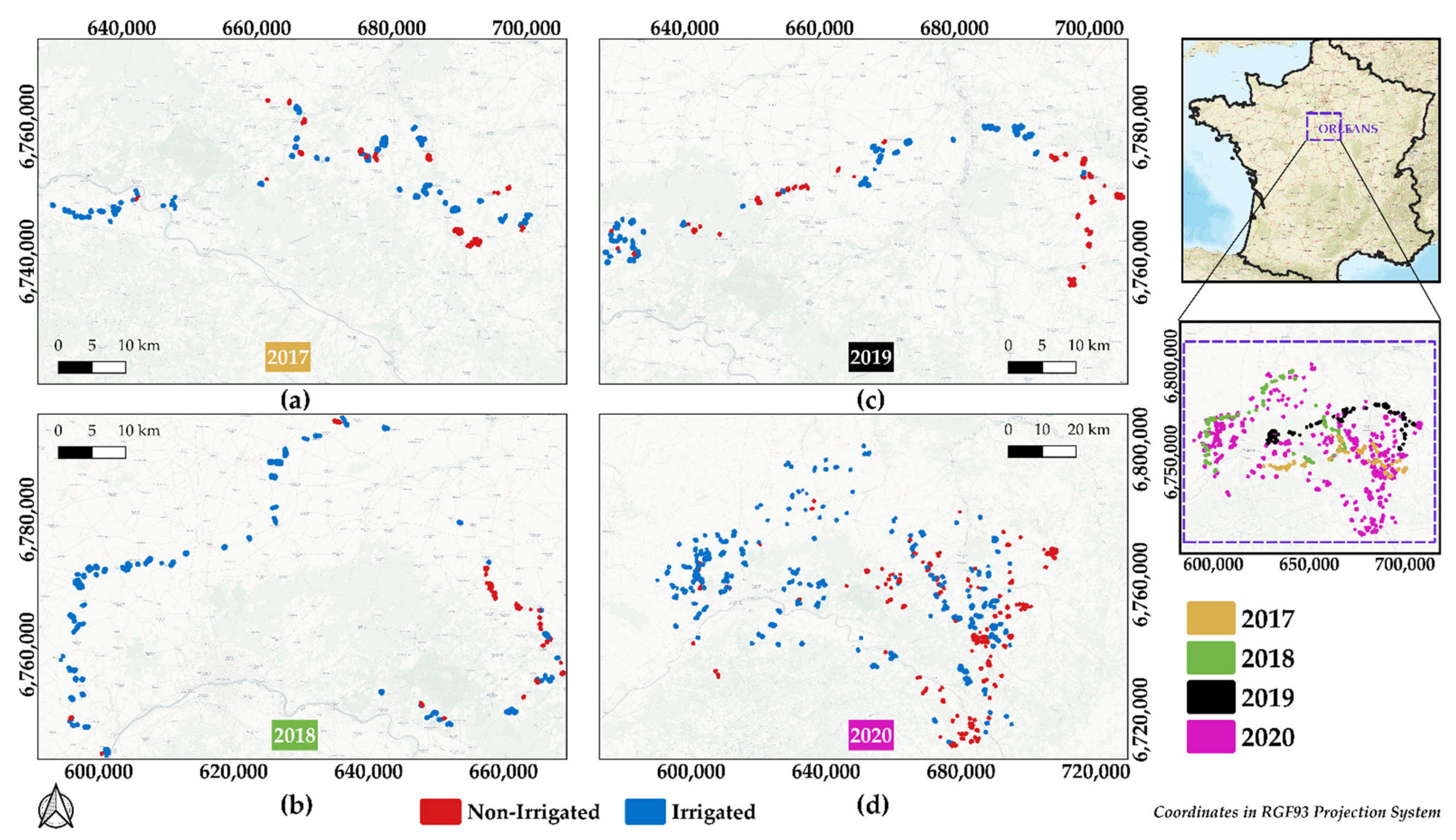
2.1. Study Site
2.2. Field Campaigns
2.3. RPG Data
2.4. Sentinel-1 SAR Data
2.5. Sentinel-2 Optical Data
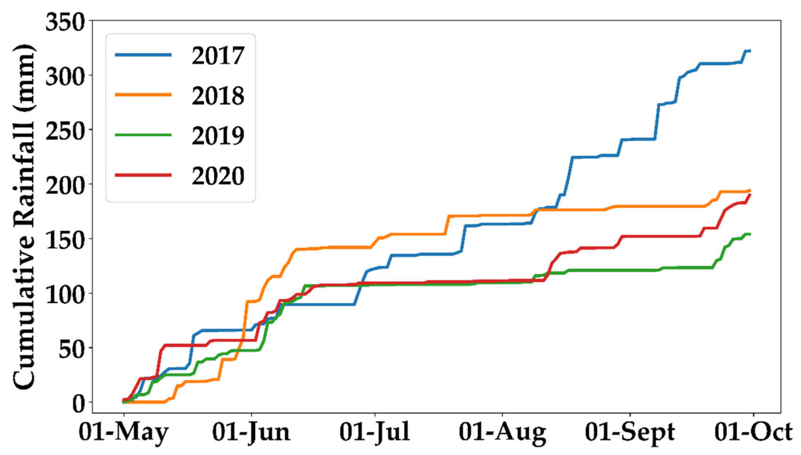
2.6. Global Precipitation Mission (GPM) Data
3. Methods
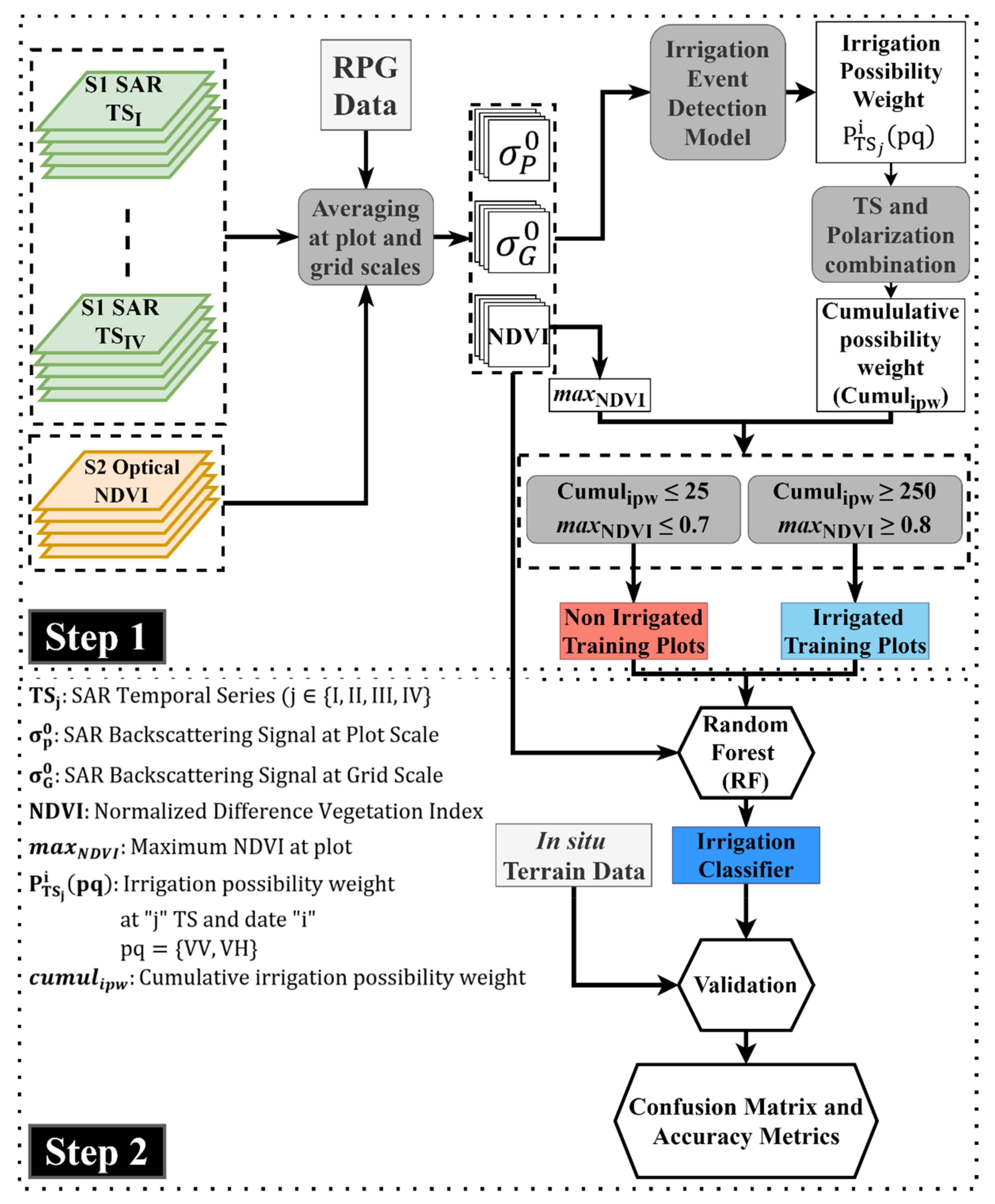
3.1. Overview
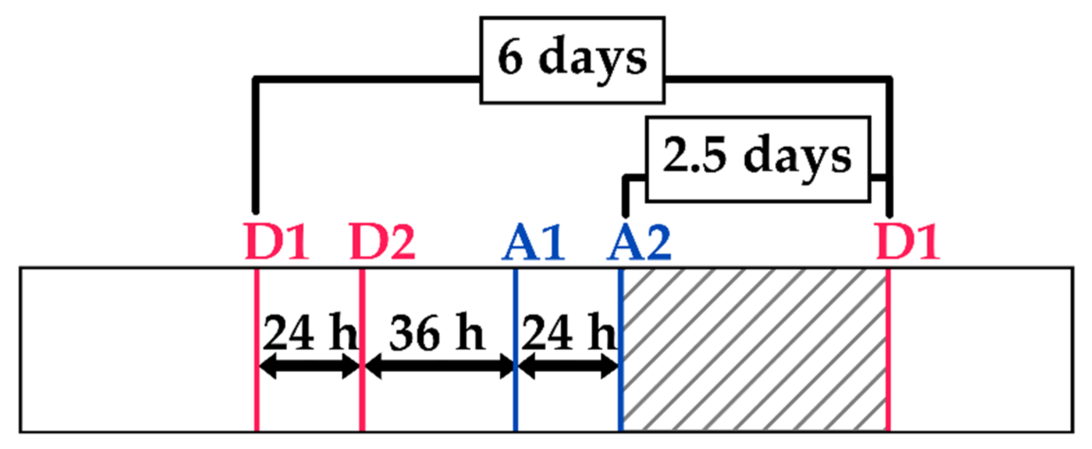
3.2. Sentinel-1 Data
3.3. Sentinel-2 Data
3.4. Training Dataset Selection Criteria
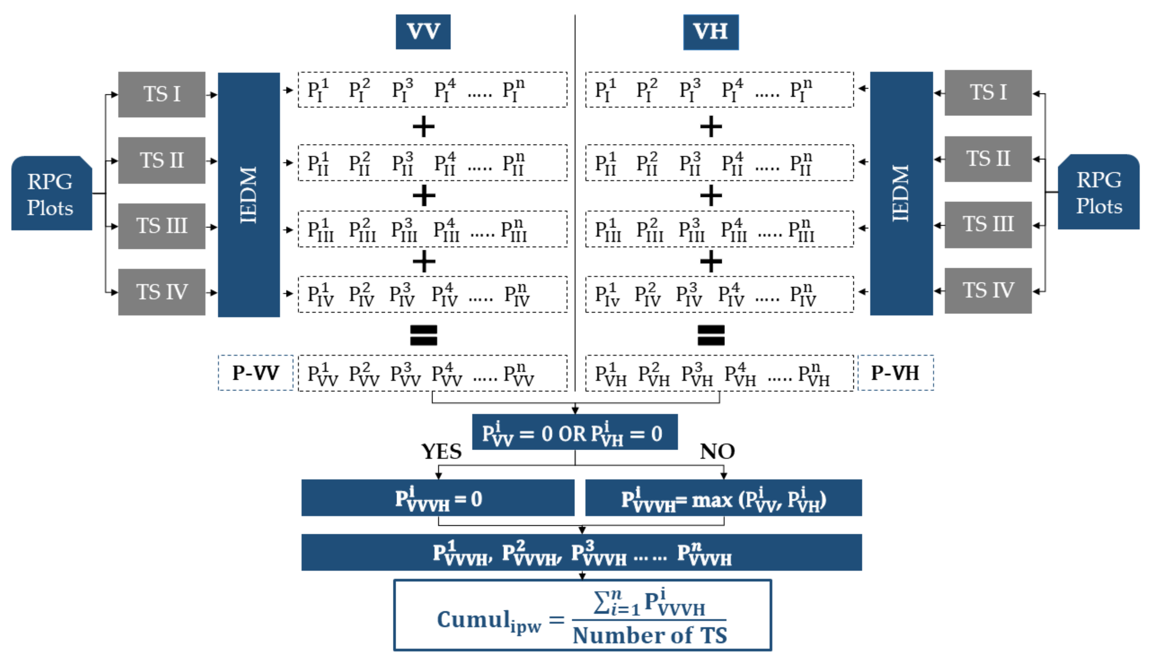
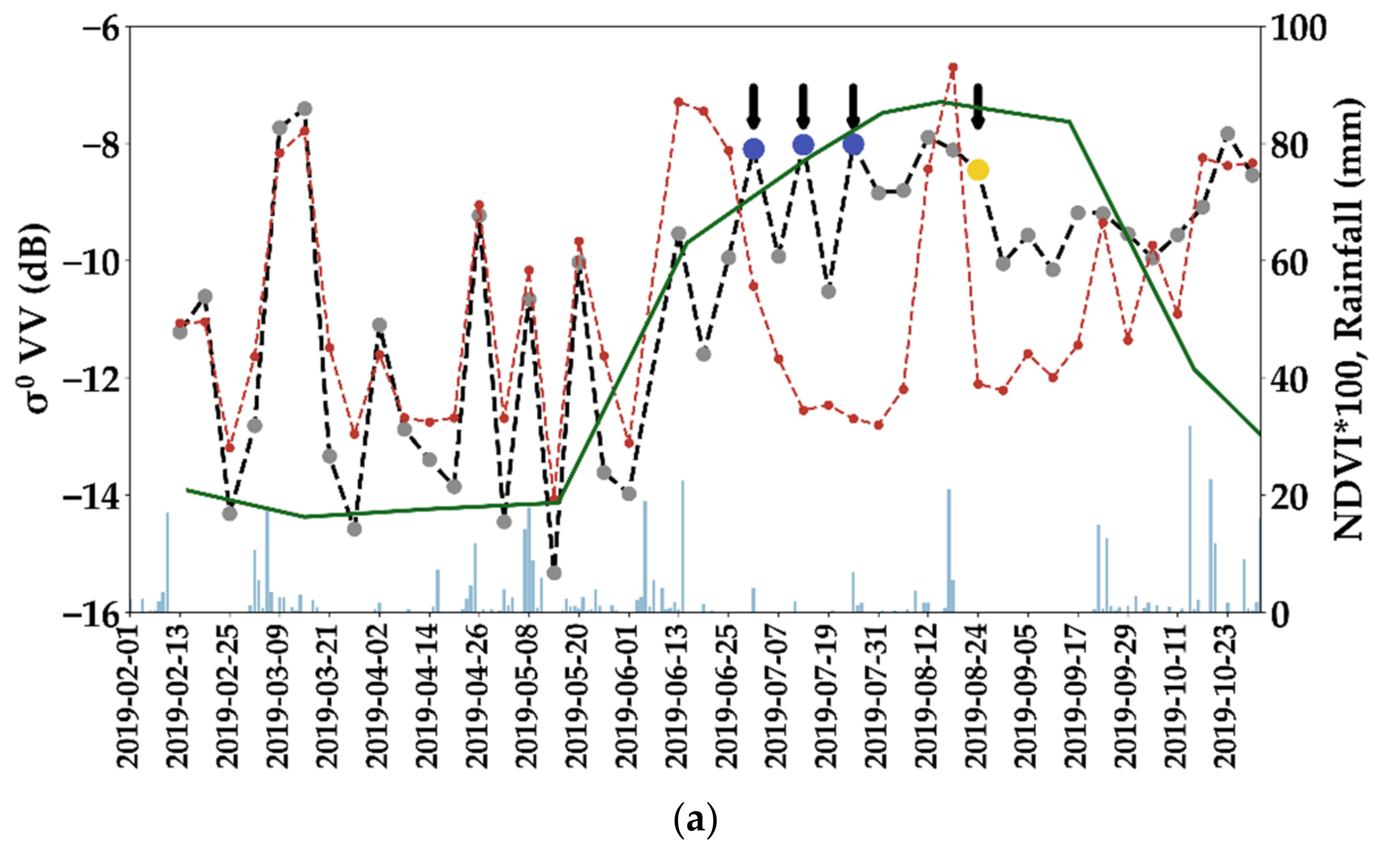
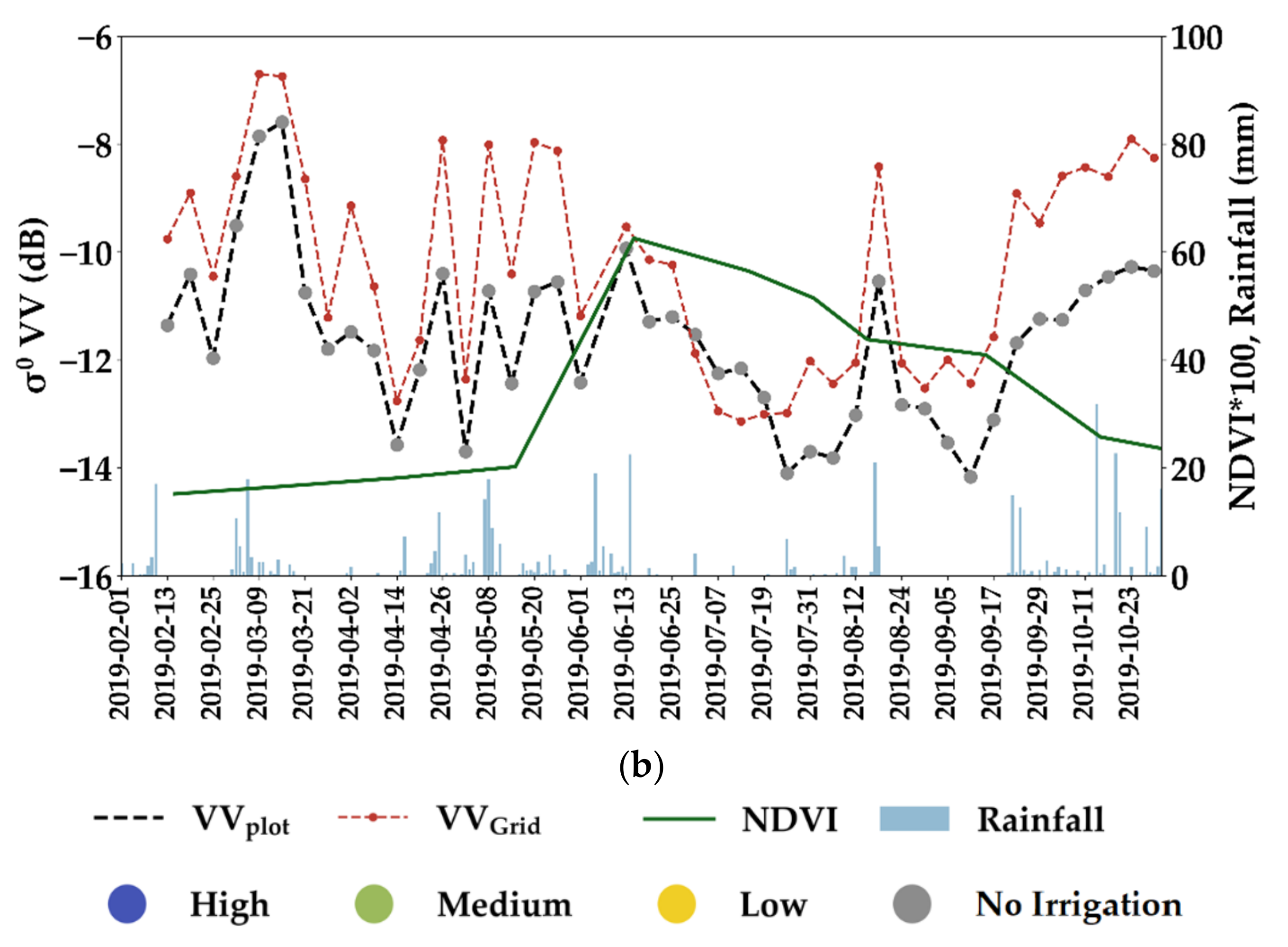
3.4.1. Irrigation Possibility Metric
3.4.2. Maximum NDVI Metric
3.4.3. Selection Criteria of Irrigated/Non-Irrigated Plots
3.5. Random Forest Classifier
3.5.1. Training Phase
3.5.2. Validation and Assessment Phase
4. Results
4.1. Irrigated vs. Non-Irrigated Plots
4.2. Comparison of Irrigation Derived Metrics Using In Situ Data
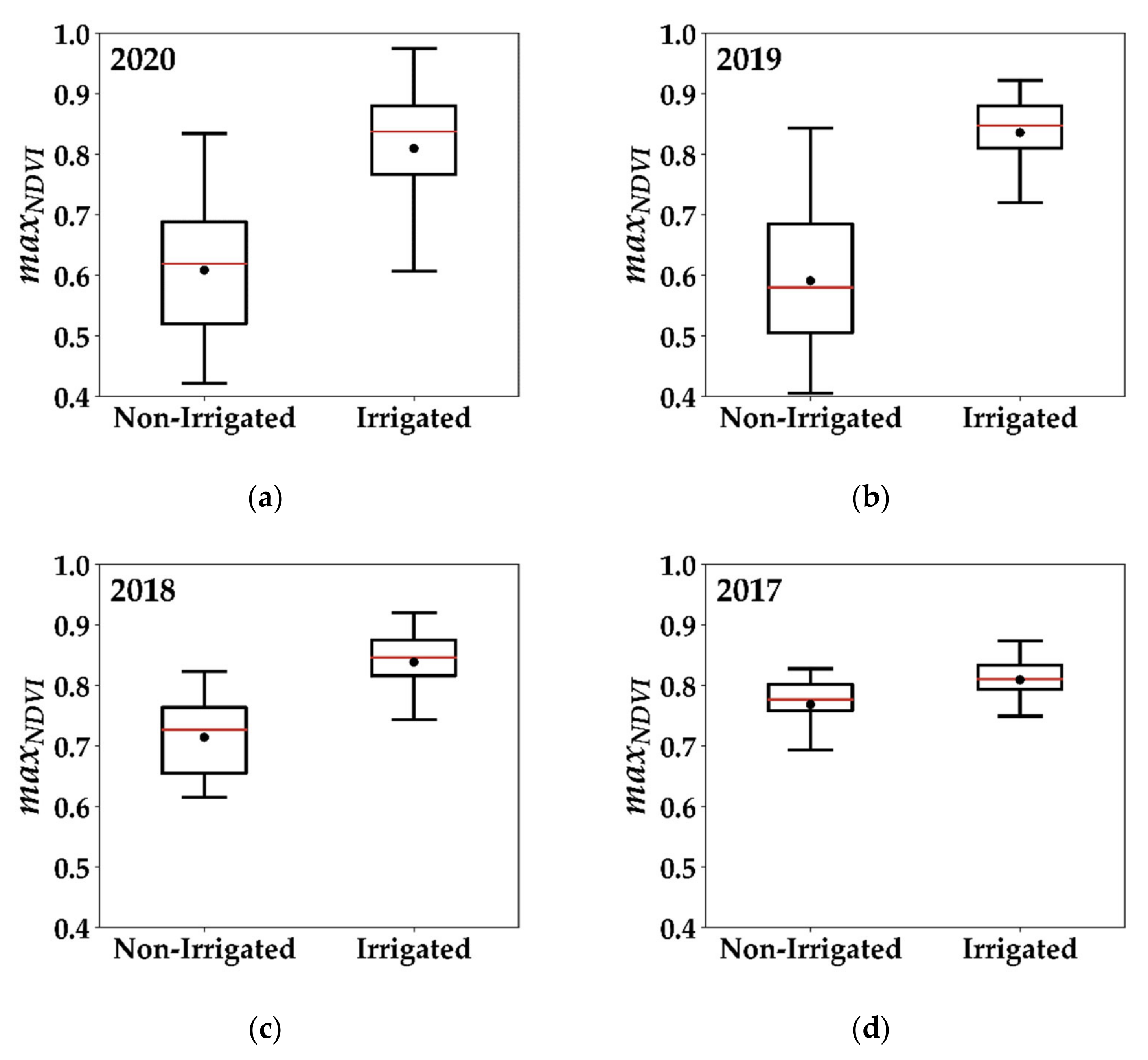
4.2.1. Maximum NDVI Value
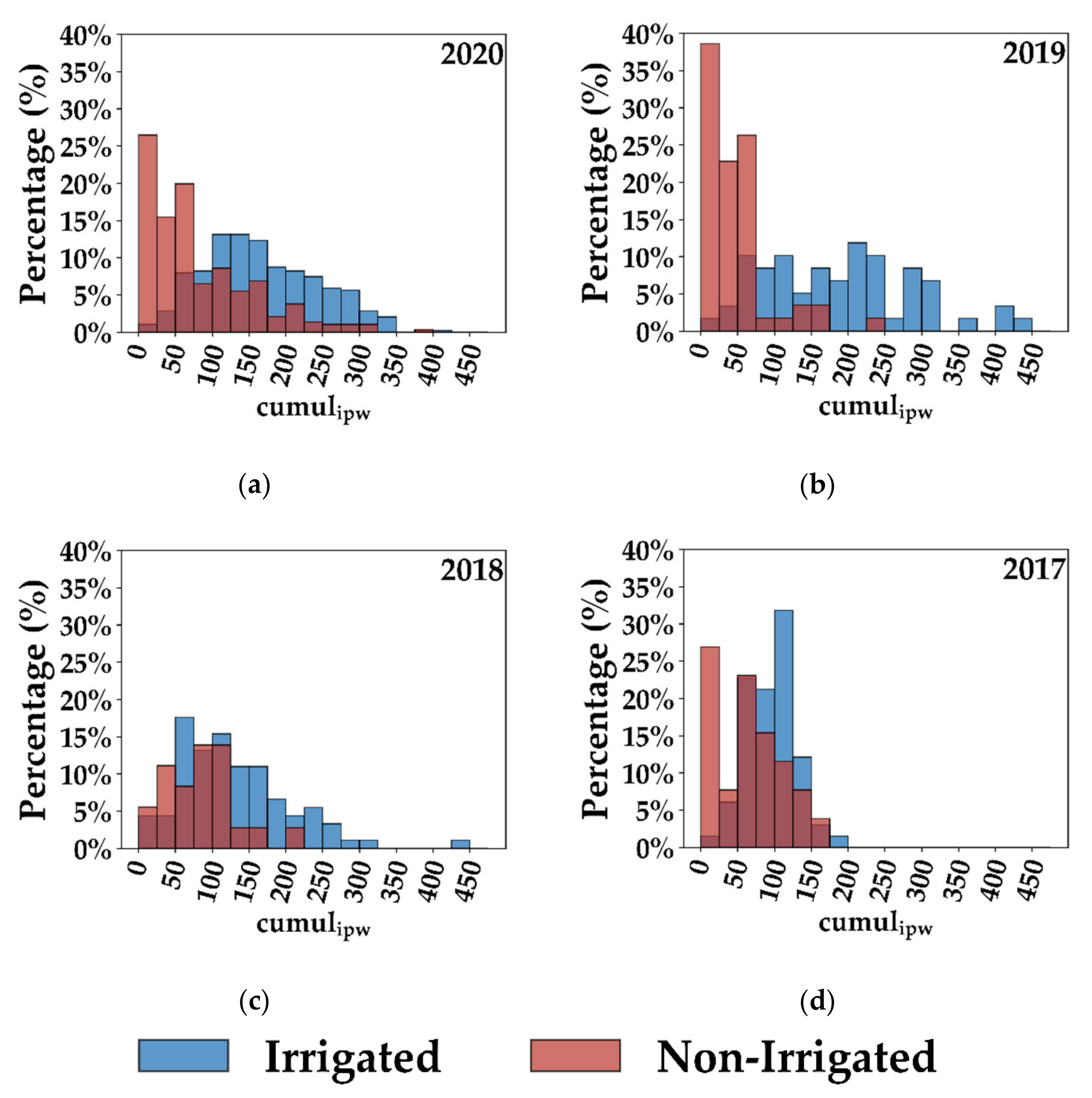
4.2.2. IEDM Cumulative Irrigation
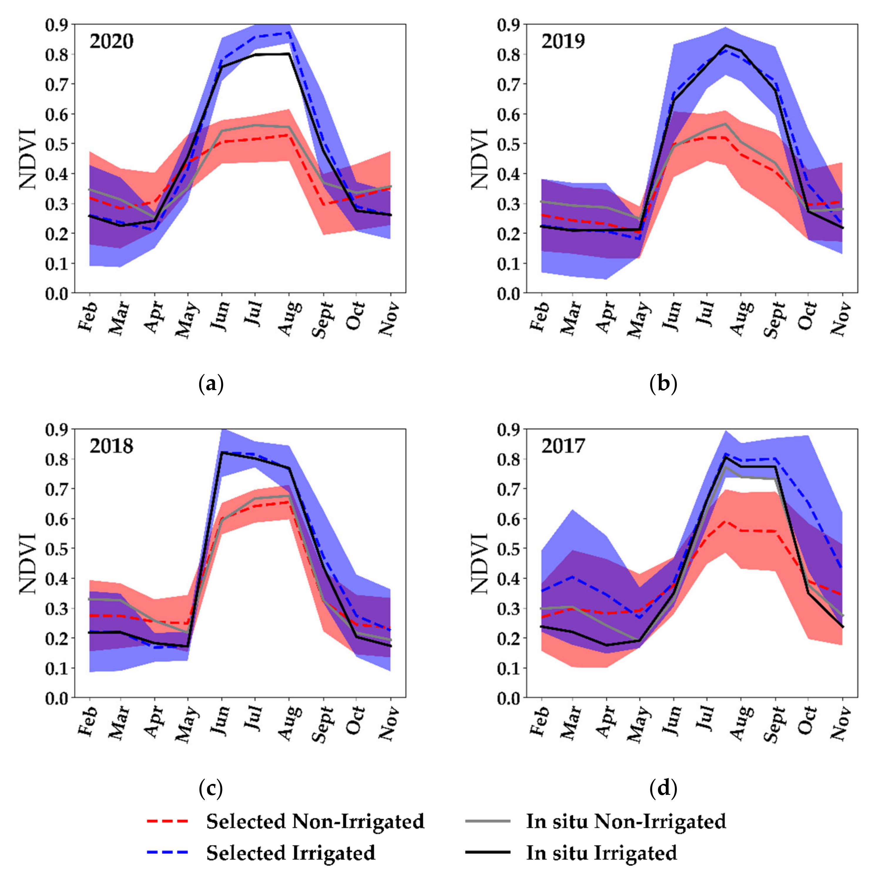
4.3. S2IM Selected Training Data
4.4. Random Forests Classification Results
4.5. Method Generalization
4.6. Thresholds Sensitivity Analysis
5. Discussion
5.1. Classification Accuracies and Rainfall Data
5.2. Limitations of
5.2.1. Threshold Values and Reference Data Selection
5.2.2. Irrigation Mapping in Humid and Dry Areas
6. Conclusions
Author Contributions
Funding
Data Availability Statement
Acknowledgments
Conflicts of Interest
References
- Grillakis, M.G. Increase in severe and extreme soil moisture droughts for Europe under climate change. Sci. Total Environ. 2019, 660, 1245–1255. [Google Scholar] [CrossRef] [PubMed]
- Harkness, C.; Semenov, M.A.; Areal, F.; Senapati, N.; Trnka, M.; Balek, J.; Bishop, J. Adverse weather conditions for UK wheat production under climate change. Agric. For. Meteorol. 2020, 282–283, 107862. [Google Scholar] [CrossRef] [PubMed]
- Richardson, K.J.; Lewis, K.H.; Krishnamurthy, P.K.; Kent, C.; Wiltshire, A.J.; Hanlon, H.M. Food security outcomes under a changing climate: Impacts of mitigation and adaptation on vulnerability to food insecurity. Clim. Chang. 2018, 147, 327–341. [Google Scholar] [CrossRef] [Green Version]
- Jamshidi, S.; Zand-Parsa, S.; Pakparvar, M.; Niyogi, D. Evaluation of Evapotranspiration over a Semiarid Region Using Multiresolution Data Sources. J. Hydrometeorol. 2019, 20, 947–964. [Google Scholar] [CrossRef]
- Tilman, D.; Balzer, C.; Hill, J.; Befort, B.L. Global food demand and the sustainable intensification of agriculture. Proc. Natl. Acad. Sci. USA 2011, 108, 20260–20264. [Google Scholar] [CrossRef] [Green Version]
- Scanlon, B.R.; Zhang, Z.; Save, H.; Sun, A.; Schmied, H.M.; van Beek, L.P.H.; Wiese, D.N.; Wada, Y.; Long, D.; Reedy, R.C.; et al. Global models underestimate large decadal declining and rising water storage trends relative to GRACE satellite data. Proc. Natl. Acad. Sci. USA 2018, 115, E1080–E1089. [Google Scholar] [CrossRef] [PubMed] [Green Version]
- FAO. Water for Sustainable Food and Agriculture; FAO: Rome, Italy, 2017; ISBN 978-92-5-109977-3. [Google Scholar]
- Bruinsma, J. The Resource Outlook to 2050: By How Much Do Land, Water and Crop Yields Need to Increase by 2050. Expert Meet. How Feed World 2009, 2050, 24–26. [Google Scholar]
- Portmann, F.T.; Siebert, S.; Döll, P. MIRCA2000-Global monthly irrigated and rainfed crop areas around the year 2000: A new high-resolution data set for agricultural and hydrological modeling. Glob. Biogeochem. Cycles 2010, 24. [Google Scholar] [CrossRef]
- Ozdogan, M.; Yang, Y.; Allez, G.; Cervantes, C. Remote Sensing of Irrigated Agriculture: Opportunities and Challenges. Remote Sens. 2010, 2, 2274–2304. [Google Scholar] [CrossRef] [Green Version]
- Siebert, S.; Döll, P.; Hoogeveen, J.; Faures, J.-M.; Frenken, K.; Feick, S. Development and validation of the global map of irrigation areas. Hydrol. Earth Syst. Sci. 2005, 9, 535–547. [Google Scholar] [CrossRef]
- Thenkabail, P.S.; Dheeravath, V.; Biradar, C.M.; Gangalakunta, O.R.P.; Noojipady, P.; Gurappa, C.; Velpuri, M.; Gumma, M.; Li, Y. Irrigated Area Maps and Statistics of India Using Remote Sensing and National Statistics. Remote Sens. 2009, 1, 50–67. [Google Scholar] [CrossRef] [Green Version]
- El Hajj, M.; Baghdadi, N.; Belaud, G.; Zribi, M.; Cheviron, B.; Courault, D.; Hagolle, O.; Charron, F. Irrigated Grassland Monitoring Using a Time Series of TerraSAR-X and COSMO-SkyMed X-Band SAR Data. Remote Sens. 2014, 6, 10002–10032. [Google Scholar] [CrossRef] [Green Version]
- Pageot, Y.; Baup, F.; Inglada, J.; Baghdadi, N.; Demarez, V. Detection of Irrigated and Rainfed Crops in Temperate Areas Using Sentinel-1 and Sentinel-2 Time Series. Remote Sens. 2020, 12, 3044. [Google Scholar] [CrossRef]
- Gao, Q.; Zribi, M.; Escorihuela, M.J.; Baghdadi, N.; Segui, P.Q. Irrigation Mapping Using Sentinel-1 Time Series at Field Scale. Remote Sens. 2018, 10, 1495. [Google Scholar] [CrossRef] [Green Version]
- Bazzi, H.; Baghdadi, N.; Ienco, D.; El Hajj, M.; Zribi, M.; Belhouchette, H.; Escorihuela, M.J.; Demarez, V. Mapping Irrigated Areas Using Sentinel-1 Time Series in Catalonia, Spain. Remote Sens. 2019, 11, 1836. [Google Scholar] [CrossRef] [Green Version]
- Segarra, J.; Buchaillot, M.L.; Araus, J.L.; Kefauver, S.C. Remote Sensing for Precision Agriculture: Sentinel-2 Improved Features and Applications. Agronomy 2020, 10, 641. [Google Scholar] [CrossRef]
- Ndikumana, E.; Minh, D.H.T.; Baghdadi, N.; Courault, D.; Hossard, L. Deep Recurrent Neural Network for Agricultural Classification using multitemporal SAR Sentinel-1 for Camargue, France. Remote Sens. 2018, 10, 1217. [Google Scholar] [CrossRef] [Green Version]
- Fayad, I.; Baghdadi, N.; Bazzi, H.; Zribi, M. Near Real-Time Freeze Detection over Agricultural Plots Using Sentinel-1 Data. Remote Sens. 2020, 12, 1976. [Google Scholar] [CrossRef]
- Bazzi, H.; Baghdadi, N.; El Hajj, M.; Zribi, M.; Minh, D.H.T.; Ndikumana, E.; Courault, D.; Belhouchette, H. Mapping Paddy Rice Using Sentinel-1 SAR Time Series in Camargue, France. Remote Sens. 2019, 11, 887. [Google Scholar] [CrossRef] [Green Version]
- Ienco, D.; Interdonato, R.; Gaetano, R.; Minh, D.H.T. Combining Sentinel-1 and Sentinel-2 Satellite Image Time Series for land cover mapping via a multi-source deep learning architecture. ISPRS J. Photogramm. Remote Sens. 2019, 158, 11–22. [Google Scholar] [CrossRef]
- Kamthonkiat, D.; Honda, K.; Turral, H.; Tripathi, N.K.; Wuwongse, V. Discrimination of irrigated and rainfed rice in a tropical agricultural system using SPOT VEGETATION NDVI and rainfall data. Int. J. Remote Sens. 2005, 26, 2527–2547. [Google Scholar] [CrossRef]
- Biggs, T.W.; Thenkabail, P.S.; Gumma, M.K.; Scott, C.; Parthasaradhi, G.R.; Turral, H.N. Irrigated area mapping in heterogeneous landscapes with MODIS time series, ground truth and census data, Krishna Basin, India. Int. J. Remote Sens. 2006, 27, 4245–4266. [Google Scholar] [CrossRef]
- Xiang, K.; Ma, M.; Liu, W.; Dong, J.; Zhu, X.; Yuan, W. Mapping Irrigated Areas of Northeast China in Comparison to Natural Vegetation. Remote Sens. 2019, 11, 825. [Google Scholar] [CrossRef] [Green Version]
- Naser, M.; Khosla, R.; Longchamps, L.; Dahal, S. Using NDVI to Differentiate Wheat Genotypes Productivity Under Dryland and Irrigated Conditions. Remote Sens. 2020, 12, 824. [Google Scholar] [CrossRef] [Green Version]
- Pervez, M.S.; Brown, J.F. Mapping Irrigated Lands at 250-m Scale by Merging MODIS Data and National Agricultural Statistics. Remote Sens. 2010, 2, 2388–2412. [Google Scholar] [CrossRef] [Green Version]
- Chen, Y.; Lu, D.; Luo, L.; Pokhrel, Y.; Deb, K.; Huang, J.; Ran, Y. Detecting irrigation extent, frequency, and timing in a heterogeneous arid agricultural region using MODIS time series, Landsat imagery, and ancillary data. Remote Sens. Environ. 2018, 204, 197–211. [Google Scholar] [CrossRef]
- Karakizi, C.; Karantzalos, K.; Vakalopoulou, M.; Antoniou, G. Detailed Land Cover Mapping from Multitemporal Landsat-8 Data of Different Cloud Cover. Remote Sens. 2018, 10, 1214. [Google Scholar] [CrossRef] [Green Version]
- Maselli, F.; Chiesi, M.; Angeli, L.; Fibbi, L.; Rapi, B.; Romani, M.; Sabatini, F.; Battista, P. An improved NDVI-based method to predict actual evapotranspiration of irrigated grasses and crops. Agric. Water Manag. 2020, 233, 106077. [Google Scholar] [CrossRef]
- Baghdadi, N.; Chaaya, J.A.; Zribi, M. Semiempirical Calibration of the Integral Equation Model for SAR Data in C-Band and Cross Polarization Using Radar Images and Field Measurements. IEEE Geosci. Remote Sens. Lett. 2010, 8, 14–18. [Google Scholar] [CrossRef] [Green Version]
- Baghdadi, N.N.; EL Hajj, M.; Zribi, M.; Fayad, I. Coupling SAR C-Band and Optical Data for Soil Moisture and Leaf Area Index Retrieval Over Irrigated Grasslands. IEEE J. Sel. Top. Appl. Earth Obs. Remote Sens. 2015, 9, 1229–1243. [Google Scholar] [CrossRef] [Green Version]
- Baghdadi, N.; Zribi, M.; Loumagne, C.; Ansart, P.; Anguela, T.P. Analysis of TerraSAR-X data and their sensitivity to soil surface parameters over bare agricultural fields. Remote Sens. Environ. 2008, 112, 4370–4379. [Google Scholar] [CrossRef] [Green Version]
- El Hajj, M.; Baghdadi, N.; Zribi, M.; Bazzi, H. Synergic Use of Sentinel-1 and Sentinel-2 Images for Operational Soil Moisture Mapping at High Spatial Resolution over Agricultural Areas. Remote Sens. 2017, 9, 1292. [Google Scholar] [CrossRef] [Green Version]
- EL Hajj, M.; Baghdadi, N.; Zribi, M.; Belaud, G.; Cheviron, B.; Courault, D.; Charron, F. Soil moisture retrieval over irrigated grassland using X-band SAR data. Remote Sens. Environ. 2016, 176, 202–218. [Google Scholar] [CrossRef] [Green Version]
- Bazzi, H.; Baghdadi, N.; El Hajj, M.; Zribi, M.; Belhouchette, H. A Comparison of Two Soil Moisture Products S2MP and Copernicus-SSM Over Southern France. IEEE J. Sel. Top. Appl. Earth Obs. Remote Sens. 2019, 12, 3366–3375. [Google Scholar] [CrossRef]
- Baghdadi, N.; Saba, E.; Aubert, M.; Zribi, M.; Baup, F. Evaluation of Radar Backscattering Models IEM, Oh, and Dubois for SAR Data in X-Band Over Bare Soils. IEEE Geosci. Remote Sens. Lett. 2011, 8, 1160–1164. [Google Scholar] [CrossRef]
- Bousbih, S.; Zribi, M.; El Hajj, M.; Baghdadi, N.; Lili-Chabaane, Z.; Gao, Q.; Fanise, P. Soil Moisture and Irrigation Mapping in A Semi-Arid Region, Based on the Synergetic Use of Sentinel-1 and Sentinel-2 Data. Remote Sens. 2018, 10, 1953. [Google Scholar] [CrossRef] [Green Version]
- Bazzi, H.; Baghdadi, N.; Fayad, I.; Charron, F.; Zribi, M.; Belhouchette, H. Irrigation Events Detection over Intensively Irrigated Grassland Plots Using Sentinel-1 Data. Remote Sens. 2020, 12, 4058. [Google Scholar] [CrossRef]
- Bazzi, H.; Baghdadi, N.; Fayad, I.; Zribi, M.; Belhouchette, H.; Demarez, V. Near Real-Time Irrigation Detection at Plot Scale Using Sentinel-1 Data. Remote Sens. 2020, 12, 1456. [Google Scholar] [CrossRef]
- Nasrallah, A.; Baghdadi, N.; El Hajj, M.; Darwish, T.; Belhouchette, H.; Faour, G.; Darwich, S.; Mhawej, M. Sentinel-1 Data for Winter Wheat Phenology Monitoring and Mapping. Remote Sens. 2019, 11, 2228. [Google Scholar] [CrossRef] [Green Version]
- El Hajj, M.; Baghdadi, N.; Bazzi, H.; Zribi, M. Penetration Analysis of SAR Signals in the C and L Bands for Wheat, Maize, and Grasslands. Remote Sens. 2018, 11, 31. [Google Scholar] [CrossRef] [Green Version]
- Zhu, X.X.; Tuia, D.; Mou, L.; Xia, G.-S.; Zhang, L.; Xu, F.; Fraundorfer, F. Deep Learning in Remote Sensing: A Comprehensive Review and List of Resources. IEEE Geosci. Remote Sens. Mag. 2017, 5, 8–36. [Google Scholar] [CrossRef] [Green Version]
- Talukdar, S.; Singha, P.; Mahato, S.; Pal, S.; Liou, Y.-A.; Rahman, A. Land-Use Land-Cover Classification by Machine Learning Classifiers for Satellite Observations—A Review. Remote Sens. 2020, 12, 1135. [Google Scholar] [CrossRef] [Green Version]
- Bazzi, H.; Ienco, D.; Baghdadi, N.; Zribi, M.; Demarez, V. Distilling Before Refine: Spatio-Temporal Transfer Learning for Mapping Irrigated Areas Using Sentinel-1 Time Series. IEEE Geosci. Remote Sens. Lett. 2020, 17, 1909–1913. [Google Scholar] [CrossRef]
- Huffman, G.; Bolvin, D.; Braithwaite, D.; Hsu, K.; Joyce, R.; Xie, P. Integrated Multi-Satellite Retrievals for GPM (IMERG), Version 4.4.; NASA’s Precipitation Processing Center: Greenbelt, MD, USA, 2014. [Google Scholar]
- Inglada, J.; Vincent, A.; Arias, M.; Tardy, B.; Morin, D.; Rodes, I. Operational High Resolution Land Cover Map Production at the Country Scale Using Satellite Image Time Series. Remote Sens. 2017, 9, 95. [Google Scholar] [CrossRef] [Green Version]
- Aubert, M.; Baghdadi, N.; Zribi, M.; Douaoui, A.; Loumagne, C.; Baup, F.; El Hajj, M.; Garrigues, S. Analysis of TerraSAR-X data sensitivity to bare soil moisture, roughness, composition and soil crust. Remote Sens. Environ. 2011, 115, 1801–1810. [Google Scholar] [CrossRef] [Green Version]
- Baghdadi, N.; El Hajj, M.; Choker, M.; Zribi, M.; Bazzi, H.; Vaudour, E.; Gilliot, J.-M.; Ebengo, D.M. Potential of Sentinel-1 Images for Estimating the Soil Roughness over Bare Agricultural Soils. Water 2018, 10, 131. [Google Scholar] [CrossRef] [Green Version]
- Brisco, B.; Brown, R.; Koehler, J.; Sofko, G.; McKibben, M. The diurnal pattern of microwave backscattering by wheat. Remote Sens. Environ. 1990, 34, 37–47. [Google Scholar] [CrossRef]
- Van Emmerik, T.; Steele-Dunne, S.C.; Judge, J.; van de Giesen, N. Impact of Diurnal Variation in Vegetation Water Content on Radar Backscatter from Maize During Water Stress. IEEE Trans. Geosci. Remote Sens. 2015, 53, 3855–3869. [Google Scholar] [CrossRef]
- Ji, L.; Peters, A.J. Assessing vegetation response to drought in the northern Great Plains using vegetation and drought indices. Remote Sens. Environ. 2003, 87, 85–98. [Google Scholar] [CrossRef]
- Kawabata, A.; Ichii, K.; Yamaguchi, Y. Global Monitoring of Interannual Changes in Vegetation Activities Using NDVI and Its Relationships to Temperature and Precipitation. Int. J. Remote Sens. 2001, 22, 1377–1382. [Google Scholar] [CrossRef]
- Potter, C.S.; Brooks, V. Global analysis of empirical relations between annual climate and seasonality of NDVI. Int. J. Remote Sens. 1998, 19, 2921–2948. [Google Scholar] [CrossRef]
- Wulder, M.A.; Hall, R.J.; Coops, N.; Franklin, S. High Spatial Resolution Remotely Sensed Data for Ecosystem Characterization. Bioscience 2004, 54, 511–521. [Google Scholar] [CrossRef] [Green Version]
- Wardlow, B.D.; Egbert, S.L. Large-area crop mapping using time-series MODIS 250 m NDVI data: An assessment for the U.S. Central Great Plains. Remote Sens. Environ. 2008, 112, 1096–1116. [Google Scholar] [CrossRef]
- Brown, J.F.; Pervez, S. Merging remote sensing data and national agricultural statistics to model change in irrigated agriculture. Agric. Syst. 2014, 127, 28–40. [Google Scholar] [CrossRef] [Green Version]
- Joseph, A.; van der Velde, R.; O’Neill, P.; Lang, R.; Gish, T. Effects of corn on C- and L-band radar backscatter: A correction method for soil moisture retrieval. Remote Sens. Environ. 2010, 114, 2417–2430. [Google Scholar] [CrossRef]
- Demarez, V.; Helen, F.; Marais-Sicre, C.; Baup, F. In-Season Mapping of Irrigated Crops Using Landsat 8 and Sentinel-1 Time Series. Remote Sens. 2019, 11, 118. [Google Scholar] [CrossRef] [Green Version]


| Year | Irrigated | Non-Irrigated | Total | Average Area (ha) |
|---|---|---|---|---|
| 2017 | 66 | 26 | 92 | 10.96 |
| 2018 | 91 | 36 | 127 | 10.34 |
| 2019 | 59 | 57 | 116 | 8.35 |
| 2020 | 395 | 291 | 686 | 7.18 |
| Total | 611 | 410 | 1021 | 8.00 |
| Year | Non-Irrigated Plots | Irrigated Plots | Total RPG Plots |
|---|---|---|---|
| 2020 | 1486 | 2209 | 19,938 |
| 2019 | 1033 | 614 | 15,958 |
| 2018 | 1441 | 1176 | 14,161 |
| 2017 | 852 | 289 | 23,599 |
| Total | 4812 | 4288 | 73,656 |
| Year | Method | OA | F_score | F_score_irr | F_score_nirr |
|---|---|---|---|---|---|
| 2020 | 84.3% | 84.1% | 86.4% | 81.3% | |
| RF in situ | 89.0% | 87.5% | 90.2% | 88.1% | |
| 2019 | 93.0% | 92.8% | 93.0% | 92.5% | |
| RF in situ | 91.3% | 91.3% | 91.2% | 91.3% | |
| 2018 | 81.8% | 82.2% | 86.8% | 70.0% | |
| RF in situ | 88.0% | 86.9% | 92.0% | 73.6% | |
| 2017 | 72.8% | 74.0% | 78.1% | 62.0% | |
| RF in situ | 78.3% | 76.5% | 85.7% | 53.7% |
| Training | |||||
|---|---|---|---|---|---|
| Validation | 2017 | 2018 | 2019 | 2020 | |
| 2017 | 61.3% | 65.1% | 65.8% | ||
| 2018 | 68.6% | 54.2% | 51.5% | ||
| 2019 | 67.1% | 53.4% | 67.4% | ||
| 2020 | 62.2% | 61.7% | 60.9% | ||
| Threshold Test | Non-Irrigated Threshold ≤ | Irrigated Threshold ≥ | F_score 2019 | F_score 2017 |
|---|---|---|---|---|
| Initial | 25 | 250 | 0.93 | 0.74 |
| Test 1 | 50 | 225 | 0.93 | 0.74 |
| Test 2 | 75 | 200 | 0.92 | 0.66 |
| Test 3 | 100 | 175 | 0.92 | 0.66 |
Publisher’s Note: MDPI stays neutral with regard to jurisdictional claims in published maps and institutional affiliations. |
© 2021 by the authors. Licensee MDPI, Basel, Switzerland. This article is an open access article distributed under the terms and conditions of the Creative Commons Attribution (CC BY) license (https://creativecommons.org/licenses/by/4.0/).
Share and Cite
Bazzi, H.; Baghdadi, N.; Amin, G.; Fayad, I.; Zribi, M.; Demarez, V.; Belhouchette, H. An Operational Framework for Mapping Irrigated Areas at Plot Scale Using Sentinel-1 and Sentinel-2 Data. Remote Sens. 2021, 13, 2584. https://doi.org/10.3390/rs13132584
Bazzi H, Baghdadi N, Amin G, Fayad I, Zribi M, Demarez V, Belhouchette H. An Operational Framework for Mapping Irrigated Areas at Plot Scale Using Sentinel-1 and Sentinel-2 Data. Remote Sensing. 2021; 13(13):2584. https://doi.org/10.3390/rs13132584
Chicago/Turabian StyleBazzi, Hassan, Nicolas Baghdadi, Ghaith Amin, Ibrahim Fayad, Mehrez Zribi, Valérie Demarez, and Hatem Belhouchette. 2021. "An Operational Framework for Mapping Irrigated Areas at Plot Scale Using Sentinel-1 and Sentinel-2 Data" Remote Sensing 13, no. 13: 2584. https://doi.org/10.3390/rs13132584
APA StyleBazzi, H., Baghdadi, N., Amin, G., Fayad, I., Zribi, M., Demarez, V., & Belhouchette, H. (2021). An Operational Framework for Mapping Irrigated Areas at Plot Scale Using Sentinel-1 and Sentinel-2 Data. Remote Sensing, 13(13), 2584. https://doi.org/10.3390/rs13132584