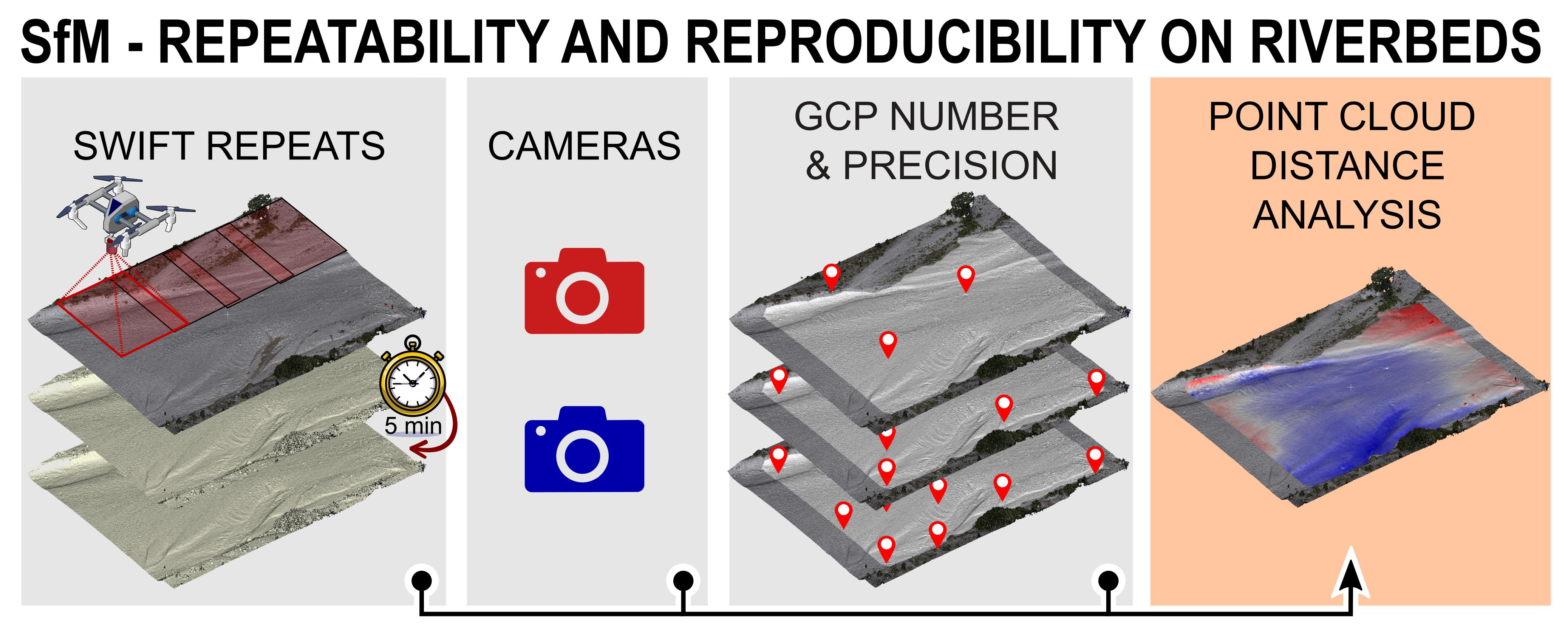
Assessing Repeatability and Reproducibility of Structure-from-Motion Photogrammetry for 3D Terrain Mapping of Riverbeds

Abstract

Structure-from-Motion (SfM) photogrammetry is increasingly employed in geomorphological applications for change detection, but repeatability and reproducibility of this methodology are still insufficiently documented. This work aims to evaluate the influence of different survey acquisition and processing conditions, including the camera used for image collection, the number of Ground Control Points (GCPs) employed during Bundle Adjustment, GCP coordinate precision and Unmanned Aerial Vehicle flight mode. The investigation was carried out over three fluvial study areas characterized by distinct morphology, performing multiple flights consecutively and assessing possible differences among the resulting 3D models. We evaluated both residuals on check points and discrepancies between dense point clouds. Analyzing these metrics, we noticed high repeatability (Root Mean Square of signed cloud-to-cloud distances less than 2.1 cm) for surveys carried out under the same conditions. By varying the camera used, instead, contrasting results were obtained that appear to depend on the study site characteristics. In particular, lower reproducibility was highlighted for the surveys involving an area characterized by flat topography and homogeneous texturing. Moreover, this study confirms the importance of the number of GCPs entering in the processing workflow, with different impact depending on the camera used for the survey.

1. Introduction

Every measurement process, with any technology, is always affected by errors, which, if not properly considered, lead to inevitable biased or wrong evaluations of the phenomenon under study. This problem is particularly relevant in the context of Change Detection (CD), which aims at recognizing differences in the state of an object over time [1,2], allowing to quantify, e.g., the effects of natural or anthropogenic events on the environment morphology. Initially based only on 2D images, in the last decades, CD has been witnessing a revolution thanks to the increasing availability of very high resolution (VHR) 3D data, provided by efficient remote sensing techniques, such as photogrammetry, Light Detection and Ranging (LiDAR) or Interferometric Synthetic Aperture Radar (InSAR). Among them, Structure-from-Motion (SfM) photogrammetry coupled with the use of Unmanned Aerial Vehicles (also known as Uncrewed Aerial Vehicles—UAVs) proved to be one of the most efficient, cost-effective technologies to generate high-quality surface reconstruction of a variety of environments [3,4].

Born from the combination of photogrammetric principles and computer vision algorithms, SfM is extensively employed for geomorphological applications, ranging from landslide [5,6] and glacier monitoring [7,8] to river channel morphology inspection [9,10] or archaeology 3D reconstructions [11,12], just to name a few. The growing use of this technique is due to several factors, including cost-effectiveness, high temporal frequency of the surveys, ease of use and automation of data processing [13]. Generating a 3D model of an area to capture its state at a certain time is often considered a simple task, that apparently requires only off-the-shelf instruments (i.e., commercial drones, consumer-grade cameras and fully automated photogrammetric software) and little training. However, to reliably detect and quantify temporal surface changes avoiding false positives [14], a deep knowledge of the data processing steps and of the uncertainties affecting the model is mandatory. To this end, several papers in the literature compared the SfM results with other VHR acquisition techniques, such as terrestrial or airborne laser scanning [3,15], or evaluated SfM accuracy on a discrete set of points, whose coordinates are measured through Global Navigation Satellite System (GNSS) [16,17]. These experiments showed centimeter to decimeter discrepancies of the SfM technique versus the compared technologies, depending on survey parameters (e.g., flight design, camera characteristics and georeferencing strategies). Moreover, some works highlighted also a dependency on the photogrammetic software used in image processing [10,18,19]. Comparing SfM results with regard to other (possibly more accurate) surveying techniques can provide an estimate of measurement accuracy and potential systematic errors, but it is not able to capture precision and repeatability [20]. The latter are fundamental aspects to quantify digital elevation model (DEM) uncertainties, which significantly affect surface change detection.

Two main approaches can be employed to estimate the precision of SfM photogrammetry. In recent years, the numerical method proposed in [21] has found extensive spread in geomorphology. It is based on Monte Carlo simulations to generate precision maps, i.e., repeated bundle adjustments are performed to evaluate the spatial variability of precision, which is influenced by photogrammetric and georeferencing conditions. This valuable tool enables the analytical assessment of error distribution for a specific survey, thus allowing to estimate the confidence intervals for detecting surface changes. However, the aforementioned simulation procedure could potentially neglect some influencing factors [20], leading to optimistic results [22]. The alternative approach is represented by the comparison of repeated surveys of the same area, performed under the same conditions during periods when no surface changes occur [20,23]. Although time-consuming, this methodology can give a comprehensive insight into the features that affect the spatial variation of precision provided by SfM photogrammetry.

Leveraging on repeated UAV surveys, in this work, we perform an extensive evaluation of SfM repeatability, defined as the variation that can be expected when surveying the same area under similar conditions (i.e., same camera, flight path, illumination conditions) within a short time interval [20,24]. Moreover, we investigate SfM reproducibility, meaning measurement variation under different conditions, by performing image acquisitions with different cameras and UAVs. In the literature, several researches demonstrate the role of GCPs on accuracy and precision of DEMs derived from SfM photogrammetry [16,23,25]. In this study, the influence of GCPs is analyzed on the one hand using different number of GCPs, and, on the other hand, exploiting 3D ground coordinates characterized by different precision. Finally, different field sites are considered, in order to evaluate how the topographic characteristics of monitored surfaces can influence the survey precision.

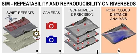
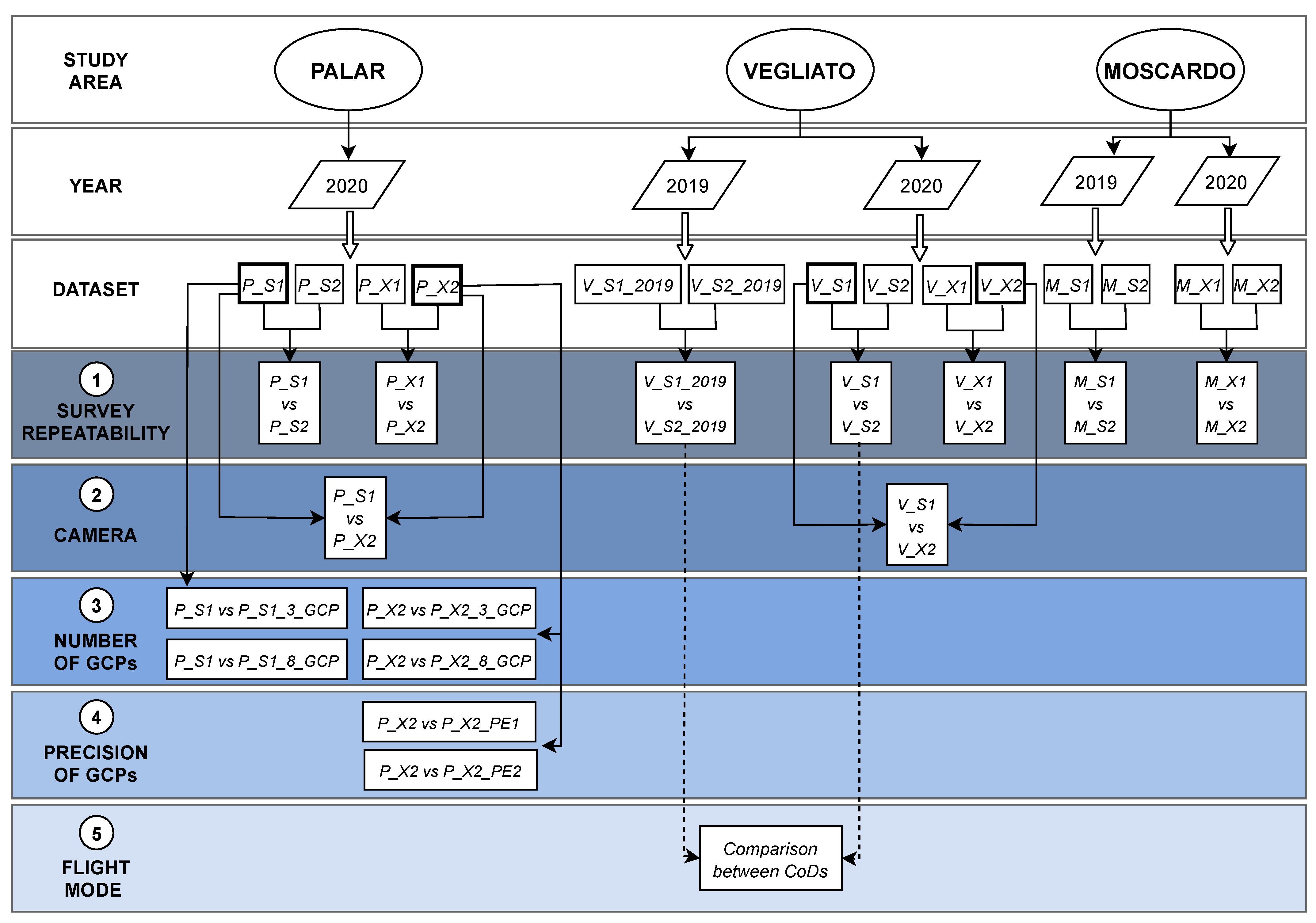
2. Materials and Methods

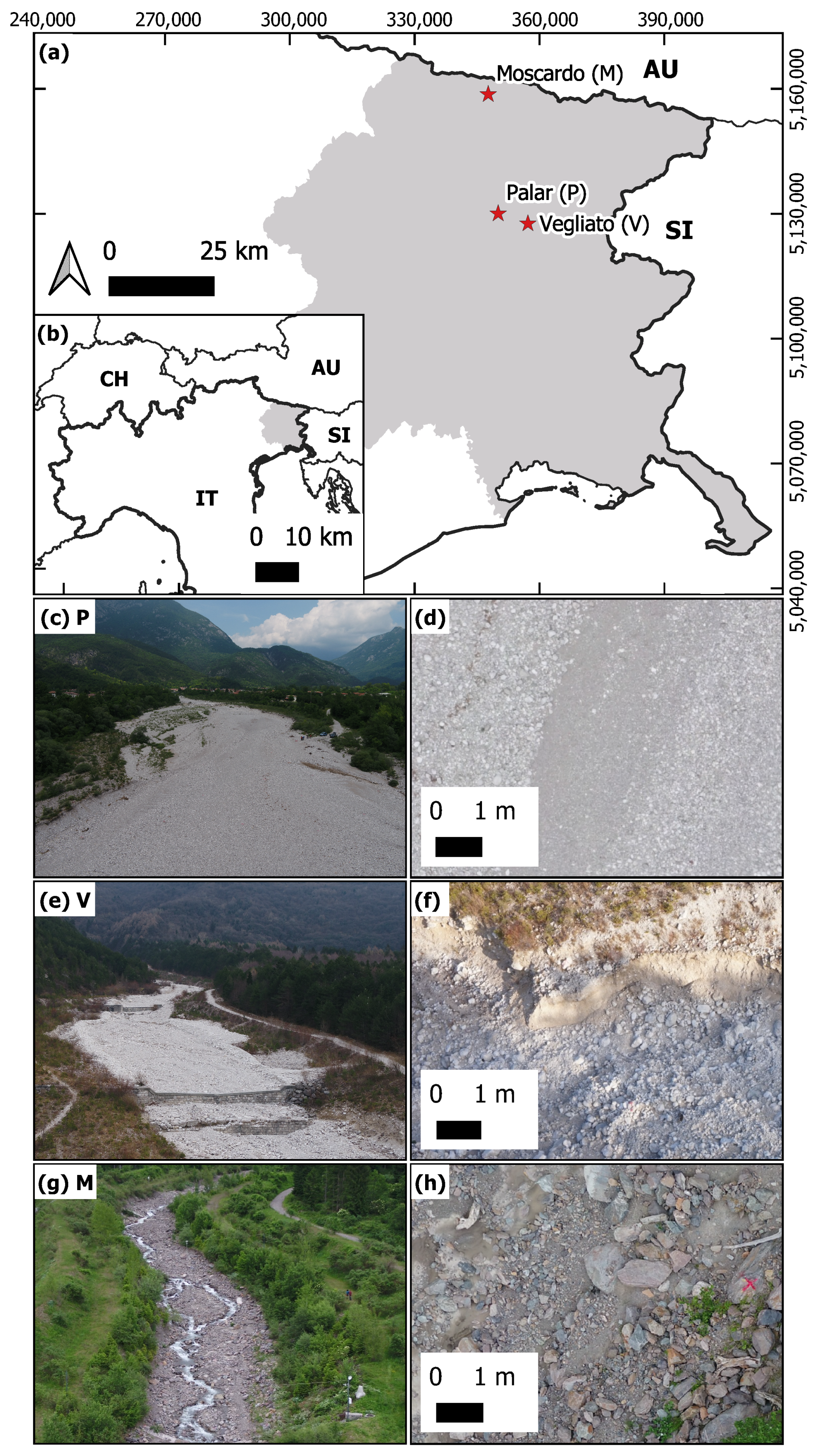
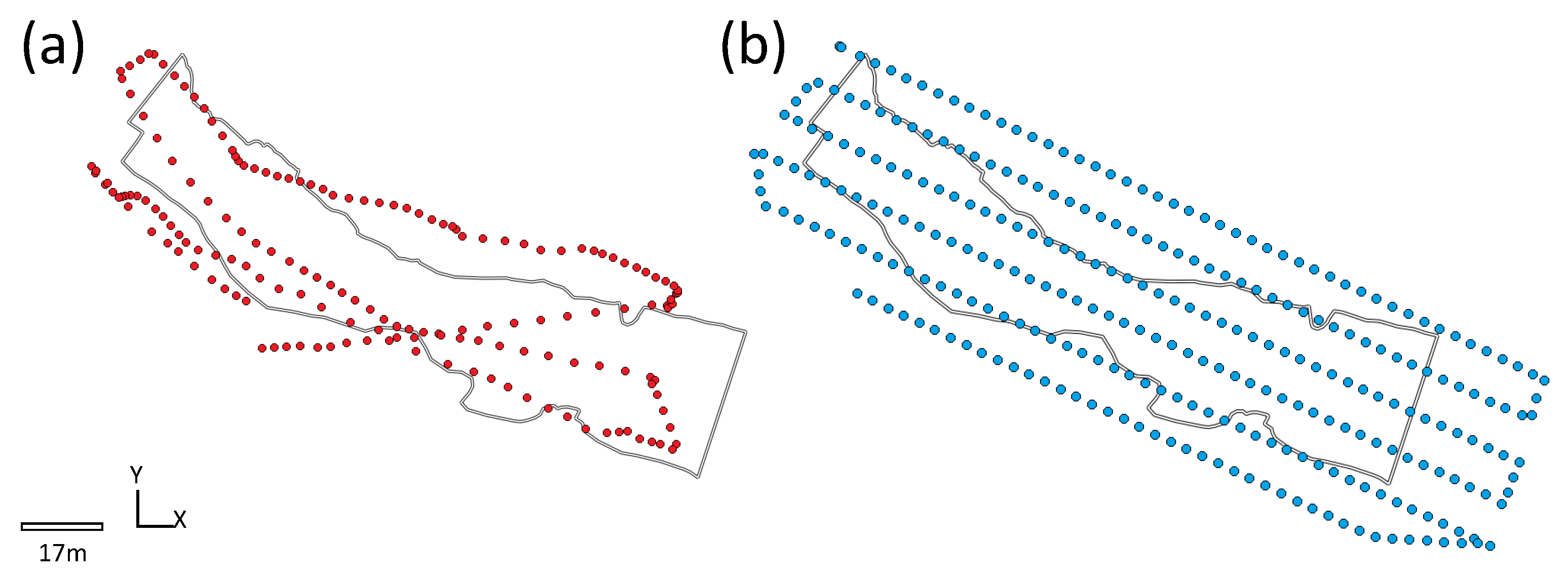
2.1. Study Areas

Three reaches (Figure 1a,b) located in Friuli Venezia Giulia region (North-east Italy) were selected as study areas due to their different geomorphological characteristics.

The first site (Palar—P) comprises 0.50 ha of the Palar Torrent (Figure 1c—46°18′31.15″N, 13°3′11.03″E) and it is mainly characterised by gentle slope bed (0.5%) with homogeneous small granulometry (Figure 1d). The second area (Vegliato—V) covers 0.41 ha of the Vegliato Torrent (Figure 1e—46°17′15.50″N, 13°8′47.95″E). This site shows more heterogeneous morphologies due to the presence of torrent control works (i.e., three check dams), river banks and fluvial terraces (Figure 1f) and the reach has a slope of 16%. The third study site (Moscardo—M) is located within the Moscardo catchment (Figure 1g—46°33′50.53″N, 13°0′43.60″E) and has an extension of 0.12 ha with a slope of 12%. This last one presents high heterogeneity in terms of roughness pattern and granulometry, with size ranging from sand to gigantic boulders, as shown in Figure 1h. This is mainly due to debris-flow events which reach very frequently the study area [26]. These particular events influence the reach morphology and cause the presence of different sediment size, from clay particles to boulders (diameter > 1 m).

2.2. Data Acquisition

Image data collection over the three study areas was carried out with two different cameras, whose characteristics are reported in

Table 1. Characteristics of the cameras employed for the surveys.

Sensor Model	Company	Resolution [MP]	Sensor Dimension [mm]	Focal Length [mm]	Image Resolution [px]
$\alpha$5000	SONY	20.0	15.4 × 23.2	20	5456 × 3632
X5S	DJI	20.8	17.3 × 13	25	5280 × 3956

.

Two different UAVs were used, each allowing different flight modes: (i) DJI Matrice210v2 quadcopter, which enables planned flight mode; and (ii) Neutech Airvision NT-4C octorotor (manual flight). The X5S camera is natively installed on the DJI Matrice210v2 quadcopter, while the Sony camera was attached to the gimbal holder using a dedicated aluminum bar specifically crafted. The same Sony camera was attached to the NT-4C octorotor using a two axis gimbal. The installations were made assuring the camera stability along with an elastic suppression of vibrations.

Nadir images were collected with an optimal overlap of 80% in flight direction and an overlap between adjacent flight-lines of 70%. All UAV surveys performed in the same day were conducted consecutively with an interval of at most 5 min, in order to guarantee the same illumination conditions. Features characterizing each survey are reported in

Table 2. Details of data acquisition. Study site: P = Palar; V = Vegliato; M = Moscardo. Camera: S = Sony $\alpha$5000; X = X5S. Drone: MT = Matrice, NT4 = NT-4C. Flight mode: Mnl = Manual, Pln = Planned. The last four columns report the number of acquired images (Images), the number of Ground Control Points (GCPs) used in the Bundle Adjustment process, the number of Control Points (CPs) considered for results evaluation purposes and the design Ground Sampling Distance (GSD), respectively.

Study Site	Camera	Dataset	Date	Drone	Flight Mode	Flight Altitude [m a.g.l.]	Images	GCPs	CPs	GSD [mm/px]
P	S	P_S1	13 June 2020	NT4	Mnl	25	167	15	17	7
	S	P_S2	13 June 2020	NT4	Mnl	25	150	15	17	7
	X	P_X1	13 June 2020	MT	Pln	25	161	15	17	5
	X	P_X2	13 June 2020	MT	Pln	25	169	15	17	5
V	S	V_S1_2019	16 December 2019	NT4	Mnl	35	217	15	15	10
	S	V_S2_2019	16 December 2019	NT4	Mnl	35	167	15	15	10
	S	V_S1	17 December 2020	MT	Pln	35	281	15	16	10
	S	V_S2	17 December 2020	MT	Pln	35	285	15	16	10
	X	V_X1	17 December 2020	MT	Pln	35	191	15	16	8
	X	V_X2	17 December 2020	MT	Pln	35	191	15	16	8
M	S	M_S1	10 June 2019	NT4	Mnl	25	155	14	12	7
	S	M_S2	10 June 2019	NT4	Mnl	25	142	14	12	7
	X	M_X1	12 June 2020	MT	Pln	25	197	15	14	5
	X	M_X2	12 June 2020	MT	Pln	25	199	15	14	5

.

In all study areas, Ground Control Points (GCPs) and Check Points (CPs) were measured with a geodetic class GNSS receiver (GS07, Leica, Heerbrugg, Switzerland) set to collect GPS (C/A, L2C, Z track on P2 codes, L1 and L2 phases), Glonass (C/A, P2 codes, L1C and L2P phases) and Galileo (E1, E5b codes and L1, L7 phases) signal observables. This ensured good satellite geometry conditions, in terms of low Dilution of Precision (DOP) parameters, also in the presence of significant sky obstructions. The GCP surveys were carried out in stop&go Post-Processed Kinematic (PPK) mode, paying attention to avoid complete losses of lock of the signal while moving around in the field, in order to guarantee an uninterrupted kinematic session linking the various GCPs. Point positions were also collected in Network Real-Time Kinematic (NRTK) mode for comparison and as a real time prediction of the achieved accuracy, while acquiring raw observations of codes and phases of visible satellites for post-processing purposes.

For every GCP the occupation time lasted from 45 to 150 s, with the antenna pole kept stable by an adjustable bipod, in order to obtain a 3D estimated precision better than 1 cm. The selected reference system for the datasets was RDN2008/UTM zone 33 (EPSG:6708). Both GCPs and CPs were uniformly distributed inside the study areas to prevent and mitigate systematic errors in the photogrammetric model [27].

2.3. Data Processing

In order to generate a 3D model for each survey, the Structure-from-Motion algorithm implemented in the Metashape software (v 1.6.4 build 10928, Agisoft LLC, St. Petersburg, Russia) was applied to process each set of collected images, simultaneously estimating exterior orientation parameters and camera calibration. In fact, no information related to interior parameters were available, and self-calibration was performed to compute, for each survey, focal length f, principal point position $(c_x,c_y)$, affinity ($b_1$), non-orthogonality ($b_2$), radial $(k_1,k_2,k_3,k_4)$ and tangential distortion parameters $(p_1,p_2)$. The estimated SfM solution was then refined (and georeferenced) exploiting the surveyed GCPs, that were used as constraints in the final bundle adjustment step. The number of GCPs employed for each image set is shown in Table 2. GNSS raw data were processed in PPK mode using the Leica GeoOffice software (LGO v 8.4, Leica Geosystems, Switzerland) referring measures to a nearby Continuously Operating Reference Station (CORS), ZUOF, for the Moscardo site and to a virtual reference station inside the study area for the Vegliato and Palar cases. The reference station data were provided in RINEX format from the GNSS networks services operating in the Friuli Venezia Giulia Region (FVG Marussi, INOGS FredNet and HxGN SmartNet). In this way, the final GCP coordinates were estimated based primarily on the PPK solutions, obtaining GCP positions with accuracy and precision of approximately 10 mm, significantly more reliable than those obtained in NRTK. We therefore used this value to set the “marker accuracy” parameter in Metashape, in order to assign proper weights to the GCP observations in the bundle adjustment [25].

A dense point cloud was then generated via the Multi-View Stereo algorithm of Metashape, exploiting the half-resolution version of the original images and applying mild filtering to remove noisy points. Furthermore, vegetation and wet surfaces were manually removed from the obtained dense point cloud to avoid biased results in the final comparisons.

For each study site, distances between point clouds generated from different image sets were computed using the M3C2 distance plugin (Multiscale Model to Model Cloud Comparison) [28] available in the Cloud Compare software (v. 2.9.1, GPL software, retrieved from http://www.cloudcompare.org, (accessed on 19 January 2021)). For each pair of compared clouds, the resulted CoD (Cloud of Difference) was rasterized at 0.02 m grid resolution for statistical analysis and visualisation purposes. Surveys performed on the same day over the same study area were conducted consecutively within short time intervals; therefore, no surface changes occurred during data collection. Distances highlighted by the cloud-to-cloud comparisons can thus be ascribed to differences arising during the photogrammetric pipeline (including image collection). Figure 2 illustrates the analyses carried out for each study area.

As already mentioned in Section 1, survey repeatability was tested comparing the results provided by two data acquisitions performed consecutively with the same camera. Moreover, for the Palar and Vegliato areas, the SfM reproducibility was assessed based on repeated data collection with two distinct cameras (within short time interval) and analyzing the differences between the derived point clouds (Figure 2—block 2).

The effects of GCPs on the precision of the final model were instead evaluated choosing the Palar area as study case. In fact, due to its flat topography and homogeneous texture, this site potentially represents the most challenging scenario for SfM reconstruction, where the benefits provided by the use of GCPs could be more relevant. In particular, one image set acquired with the $\alpha$5000 Sony camera and one collected with the Zenmuse X5S were considered and processed from scratch using two subsets of GCPs in the bundle adjustment (3 and 8 GCPs, respectively). The resulting point clouds (P_S1_3_GCP and P_S1_8_GCP for the Sony camera; P_X2_3_GCP and P_X2_8_GCP for the X5S camera) were compared with the corresponding reference ones (P_S1 and P_X2, respectively) obtained with 15 GCPs (Figure 2—block 3). The photogrammetric model can be influenced not only by the number of GCPs introduced as constraints in the bundle adjustment, but also by the GCP coordinate precision. To test this aspect, we synthetically generated two more cases for the P_X2 dataset, in which the GNSS coordinates of the 15 GCPs were perturbed by adding random Gaussian noise of zero mean and standard deviation $\sigma$. In the first one (P_X2_PE1), ${\sigma }_{xy}=1$ cm and ${\sigma }_z=2$ cm were employed for the planimetric and altimetric components, respectively, while in the latter (P_X2_PE2) ${\sigma }_{xy}=2$ cm and ${\sigma }_z=4$ cm were selected (Figure 2—block 4).

Finally, the impact of UAV flight mode was analyzed for the Vegliato study area comparing two CoDs resulting from the surveys conducted in 2019 and 2020 (Figure 2—block 5). The models and the corresponding CoDs were derived from datasets acquired with the same camera (Sony) and at the same flight altitude (35 m agl). However, the 2019 surveys (dubbed V_S1_2019 and V_S2_2019) were performed with the NT-4C octorotor in manual flight mode, whereas the images acquired in 2020 were captured using the planned flight mode provided by the DJI Matrice210v2 quadcopter. We highlight that, for this test, only an indirect analysis on the CoDs was possible. In fact, a direct comparison between models deriving from different flight modes was impractical due to surface changes that occurred between the 2019 and 2020 data collections.

3. Results

Hereinafter, the results for each dataset and the comparisons among the obtained models are reported in detail.

Table 3. Estimated camera parameter values for all datasets. In the last column the actual mean GSD is reported, computed after the image orientation stage.

Study Site	Dataset	f [px]	${\mathit{c}}_{\mathit{x}}$ [px]	${\mathit{c}}_{\mathit{y}}$ [px]	${\mathit{b}}_1$ [–]	${\mathit{b}}_2$ [–]	${\mathit{k}}_1$ [$·{10}^{-2}$]	${\mathit{k}}_2$ [$·{10}^{-2}$]	${\mathit{k}}_3$ [$·{10}^{-2}$]	${\mathit{k}}_4$ [$·{10}^{-2}$]	${\mathit{p}}_1$ [$·{10}^{-3}$]	${\mathit{p}}_2$ [$·{10}^{-3}$]	Reprj. err. [px]	GSD [mm/px]
P	P_S1	4780.6	−24.0	2.7	−0.28	−0.23	−15.2	11.4	5.1	−3.6	−0.8	0.7	0.66	9
	P_S1_8_GCP	4791.4	−24.0	2.5	−0.28	−0.19	−15.2	11.6	5.1	−3.6	−0.8	0.7	0.67	9
	P_S1_3_GCP	4791.2	−24.0	2.5	−0.28	−0.19	−15.2	11.6	5.1	−3.6	−0.8	0.7	0.67	9
	P_S2	4818.8	−24.2	0.3	−0.28	0.83	−15.5	11.7	5.6	−3.7	−0.2	1.2	0.72	10
	P_X1	4459.0	46.7	18.9	−6.66	0.3	0.6	−4.5	12.9	−10.9	2.3	1.0	0.85	5
	P_X2	4385.1	50.4	18.9	−6.93	0.44	0.5	−3.9	10.9	−9.1	2.2	0.9	0.82	5
	P_X2_8_GCP	4378.1	49.8	18.9	−7.31	0.46	0.6	−4.5	12.4	−10.3	2.2	0.9	0.76	5
	P_X2_3_GCP	4383.5	49.6	18.8	−7.42	0.46	0.8	−4.5	12.6	−10.5	2.2	0.9	0.76	5
	P_X2_PE1	4396.9	49.3	18.7	−7.42	0.48	0.6	−4.5	12.7	−10.6	2.2	0.9	0.76	5
	P_X2_PE2	4400.5	49.2	18.6	−7.42	0.48	0.6	−4.6	12.8	−10.7	2.2	0.9	0.76	5
V	V_S1_2019	4814.8	−12.6	3.9	−0.28	1.08	−15.8	13.3	1.6	0.1	−0.7	1.1	0.70	7
	V_S2_2019	4809.9	−11.2	3.4	−0.28	0.27	−15.4	11.4	7.1	−5.7	−0.4	1.5	0.69	8
	V_S1	4801.7	−25.6	7.3	−0.28	−0.33	−15.4	11.3	6.8	−5.3	−0.6	1.1	0.69	7
	V_S2	4781.6	−33.7	−19.8	−0.28	0.83	−15.2	11.0	7.0	−5.5	−0.6	1.1	0.69	7
	V_X1	4526.2	43.8	4.6	−7.06	−0.17	−0.2	−0.2	2.1	−1.0	2.3	0.4	0.91	7
	V_X2	4578.9	39.9	5.2	−7.72	0.47	−0.5	0.2	0.6	0.9	2.1	0.4	0.87	7
M	M_S1	4812.5	−25.0	4.9	−0.28	0.83	−15.5	13.2	1.3	0.1	−0.8	1.0	1.22	8
	M_S2	4808.4	−26.2	12.7	−0.28	0.83	−15.7	13.7	0.5	0.1	−0.7	0.4	1.24	7
	M_X1	4543.2	42.8	15.0	−5.52	−1.93	−0.03	−1.3	5.0	−4.3	2.2	0.9	0.92	6
	M_X2	4541.2	43.1	14.4	−6.54	−1.47	−0.1	−0.3	1.1	0.3	2.2	0.8	0.88	6

summarizes the computed camera parameter values, that were estimated via self-calibration as previously described. It is possible to notice the variability of the focal length f estimated for consecutive surveys performed with the same camera, that reaches 74 pixels (1.7%) for the X5S datasets over the Palar area. We reported also the mean GSD computed for each image set after the SfM process. This can differ from the nominal value (Table 2) for two main reasons. Image acquisitions with the NT-4C octorotor, in fact, were performed in manual flight mode, which made it difficult to meet the design flight altitude. For the planned flights, instead, a constant altitude (above see level) had to be set in the UAV control unit, preventing the design flight altitude (above ground level) from being respected for the whole surveyed area.

The model accuracy was investigated analyzing at first the residuals on the CPs (i.e., the differences between GNSS-measured coordinates and photogrammetric ones), that give an indication also on possible georeferencing errors. In

Table 4. Residuals on Check Points (in cm). Mean value $\mu$ and standard deviation $\sigma$ are reported for each component $(X,Y,Z)$ and for the total 3D error. For the latter, mean and standard deviation are reported also as a function of the average GSD.

Study Site	Dataset	${\mathit{\mu }}_{\mathit{X}}$ [cm]	${\mathit{\sigma }}_{\mathit{X}}$ [cm]	${\mathit{\mu }}_{\mathit{Y}}$ [cm]	${\mathit{\sigma }}_{\mathit{Y}}$ [cm]	${\mathit{\mu }}_{\mathit{Z}}$ [cm]	${\mathit{\sigma }}_{\mathit{Z}}$ [cm]	${\mathit{\mu }}_{3\mathit{D}}$ [cm]	${\mathit{\sigma }}_{3\mathit{D}}$ [cm]	${\mathit{\mu }}_{3\mathit{D}}$ [GSD]	${\mathit{\sigma }}_{3\mathit{D}}$ [GSD]
P	P_S1	0.2	1.1	−0.5	1.5	0.0	1.3	2.1	0.8	2.4	1.0
	P_S1_8_GCP	0.3	1.0	−0.6	1.4	−0.1	1.2	2.0	0.8	2.3	1.0
	P_S1_3_GCP	−0.2	0.6	−0.5	2.0	0.5	1.2	2.2	0.9	2.5	1.1
	P_S2	0.4	1.2	−0.5	1.8	0.0	1.0	2.3	0.7	2.2	0.6
	P_X1	0.0	2.3	−0.2	2.5	−0.3	2.8	4.0	1.5	7.1	2.7
	P_X2	0.3	2.2	−0.1	2.6	0.4	2.8	4.0	1.8	7.7	3.5
	P_X2_8_GCP	−0.5	2.5	−0.2	2.0	−0.6	3.4	4.3	1.8	8.3	3.6
	P_X2_3_GCP	0.5	2.3	−0.4	2.3	−5.0	6.6	7.3	5.0	14.1	9.8
	P_X2_PE1	0.2	2.3	−0.1	2.4	0.1	3.0	4.0	1.7	7.8	3.3
	P_X2_PE2	0.4	2.3	−0.3	2.3	0.2	2.9	4.0	1.6	7.7	3.2
V	V_S1_2019	−0.1	1.1	0.0	1.3	0.4	1.1	1.8	0.8	2.7	1.3
	V_S2_2019	−0.6	2.0	−0.1	1.4	0.3	1.2	2.5	1.0	3.1	1.3
	V_S1	−0.1	0.8	−0.1	0.6	−0.7	1.4	1.5	1.0	2.1	1.5
	V_S2	0.0	0.8	−0.2	0.6	−0.2	0.9	1.2	0.6	1.8	0.9
	V_X1	0.3	1.6	−0.2	0.9	0.1	1.7	2.0	1.6	2.7	2.1
	V_X2	−0.1	1.0	−0.1	0.9	−0.9	1.8	2.1	0.9	2.9	1.3
M	M_S1	0.6	0.8	−0.3	0.6	0.2	1.5	1.8	0.5	2.2	0.6
	M_S2	0.4	0.7	−0.4	0.7	0.9	1.6	1.9	0.9	2.8	1.3
	M_X1	0.5	0.9	−0.3	0.5	−0.3	1.9	1.9	1.2	3.2	2.1
	M_X2	0.4	0.8	−0.3	0.5	−0.1	1.8	1.7	1.1	2.8	1.8

, the mean value $\mu$ and standard deviation $\sigma$ for CP residuals are reported for each dataset, showing both the signed residuals for the three components $(X,Y,Z)$ and the total 3D error. For the latter, the statistics are expressed also as a function of the average GSD. In the following sections, we will discuss in detail the results on CP residuals reported in Table 4.

As further figure of merit, we evaluated the distances between dense point clouds (CoDs) for precision assessment. Figure 3, Figure 4 and Figure 5 illustrate the M3C2 distance between pairs of models for the three study areas, while

Table 5. Summary statistics of M3C2 distance values for all the compared point clouds. Mean ±  standard deviation and RMS are reported (in cm).

Study Site	Reference Set	Compared Set	$\mathit{\mu }\pm \mathit{\sigma }$ [cm]	RMS [cm]
P	P_S1	P_S2	−0.1 ± 1.3	1.3
	P_X2	P_X1	−0.6 ± 0.8	1.0
	P_S1	P_X2	0.4 ± 2.6	2.6
	P_S1	P_S1_3_GCP	0.3 ± 0.8	0.9
	P_S1	P_S1_8_GCP	−0.1 ± 0.3	0.3
	P_X2	P_X2_3_GCP	−6.0 ± 8.3	10.3
	P_X2	P_X2_8_GCP	−0.7 ± 1.0	1.2
	P_X2	P_X2_PE1	−0.2 ± 0.5	0.6
	P_X2	P_X2_PE2	−0.2 ± 0.8	0.8
V	V_S1_2019	V_S2_2019	0.5 ± 1.2	1.3
	V_S1	V_S2	0.6 ± 0.7	1.0
	V_X1	V_X2	−1.7 ± 1.3	2.1
	V_S1	V_X2	0.2 ± 1.5	1.5
M	M_S1	M_S2	−0.6 ± 1.2	1.4
	M_X1	M_X2	0.1 ± 0.5	0.5

shows the corresponding statistics.

The outcomes are detailed in the following describing separately (i) survey repeatability and the use of different cameras, (ii) different number of GCPs and varying GCP coordinate precision, and (iii) different flight modes.

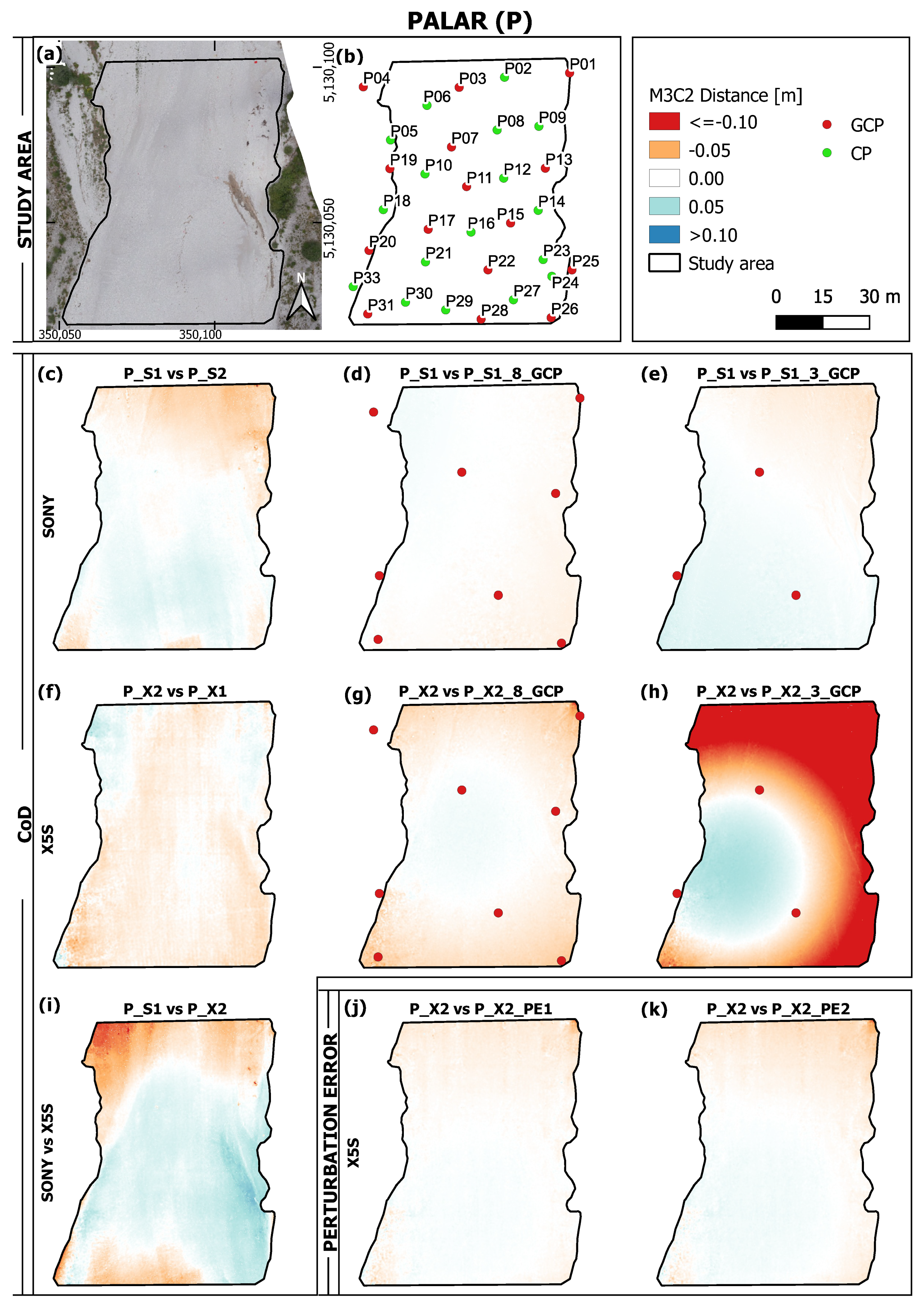
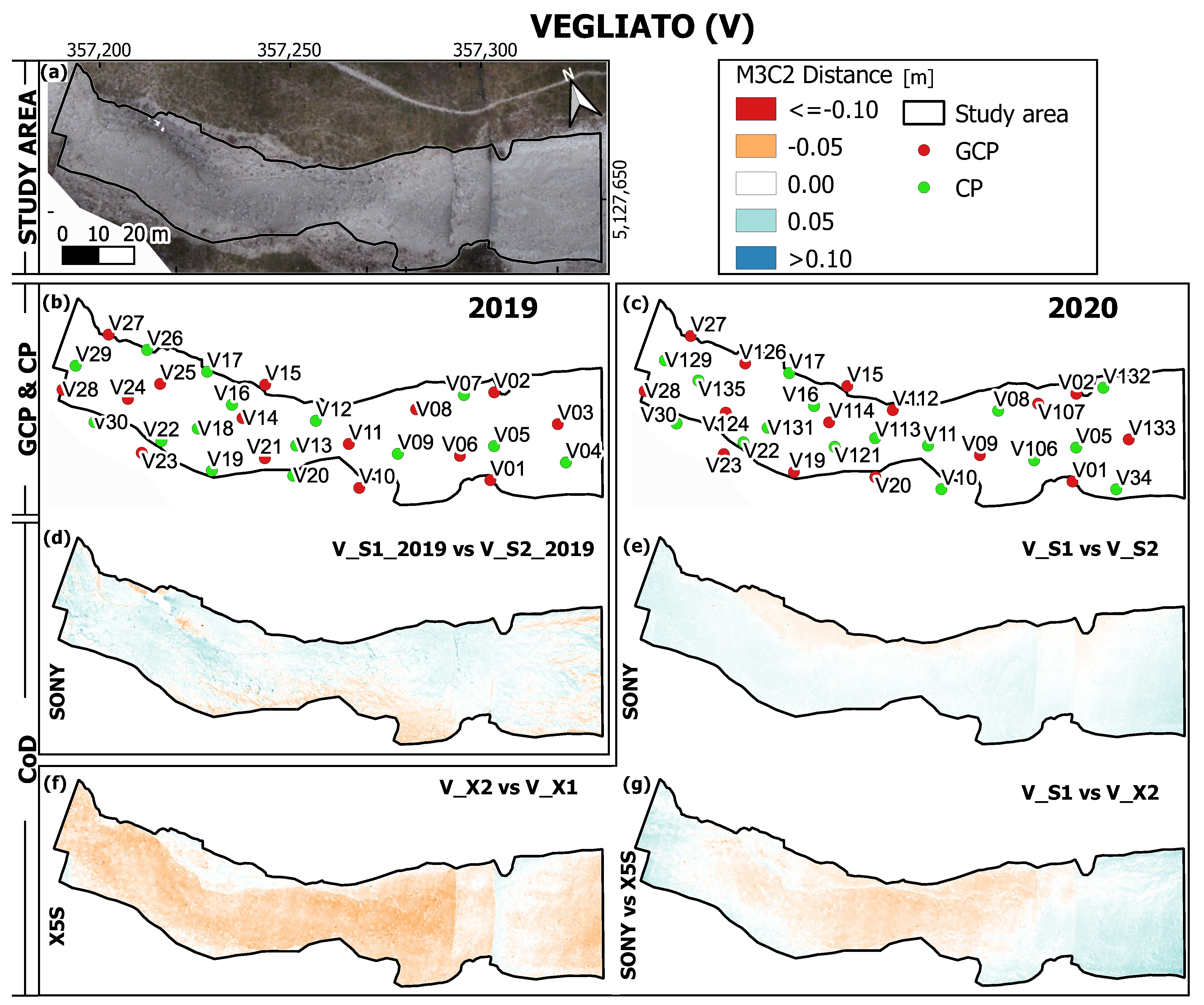
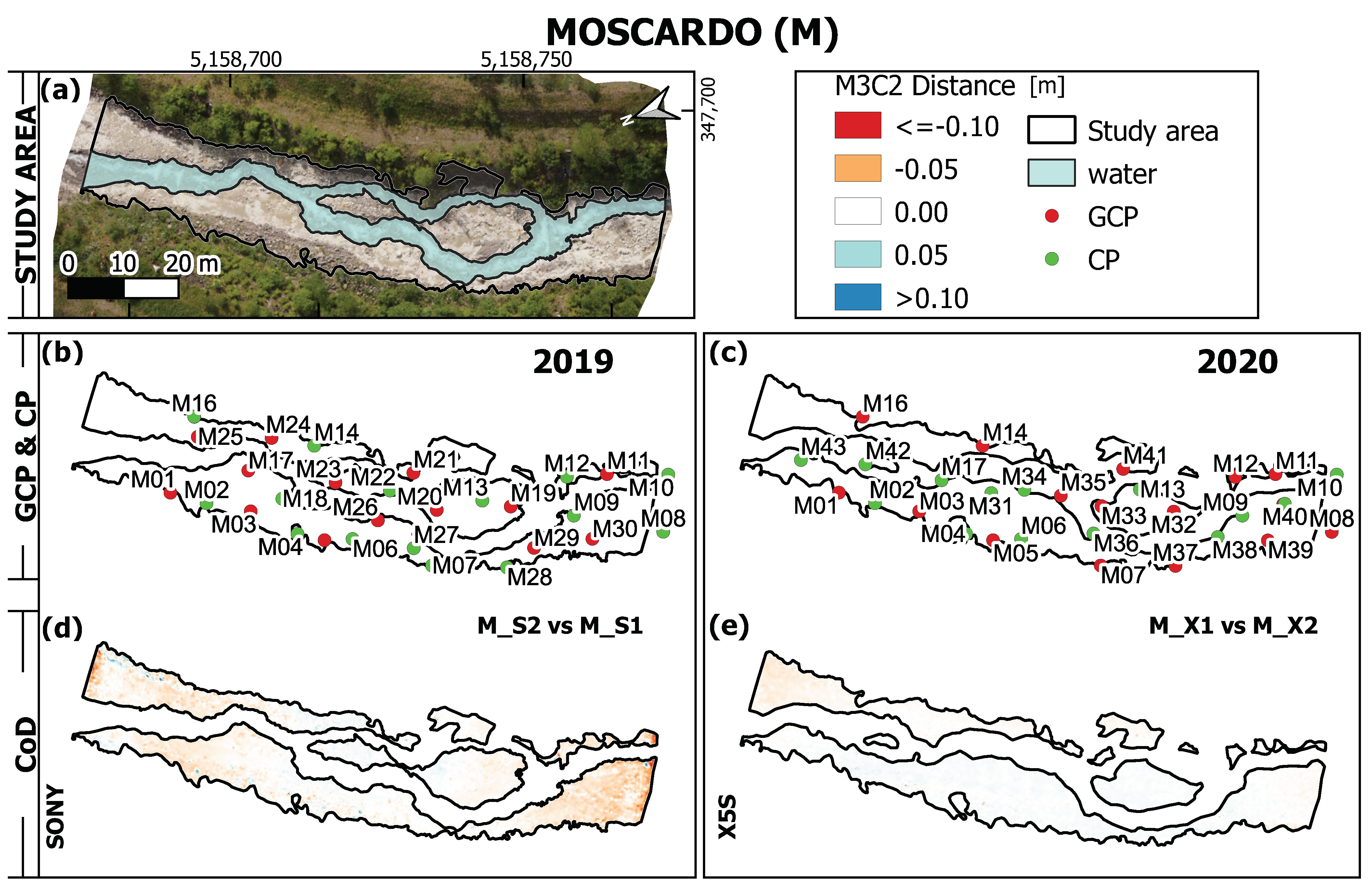
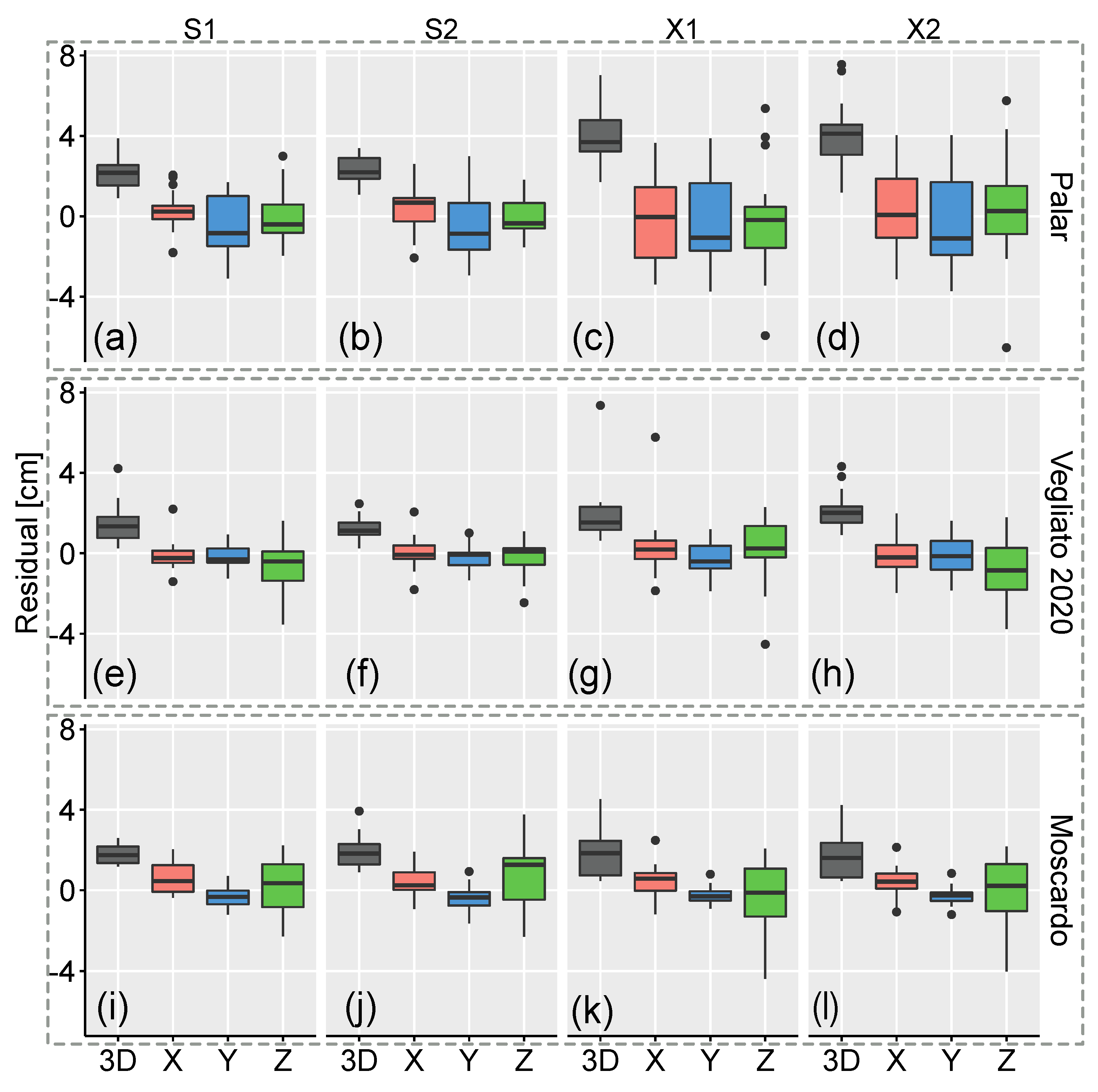
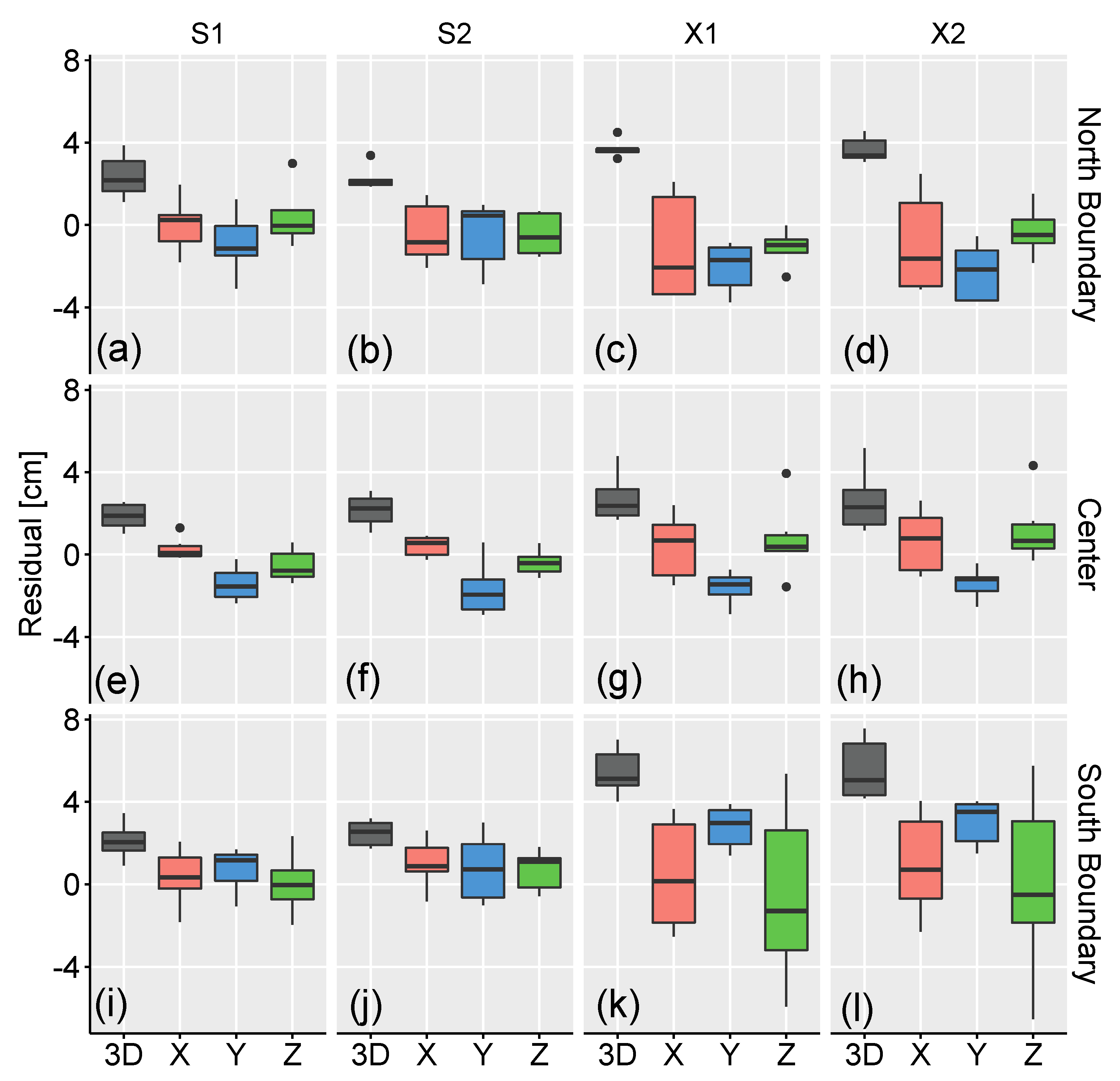
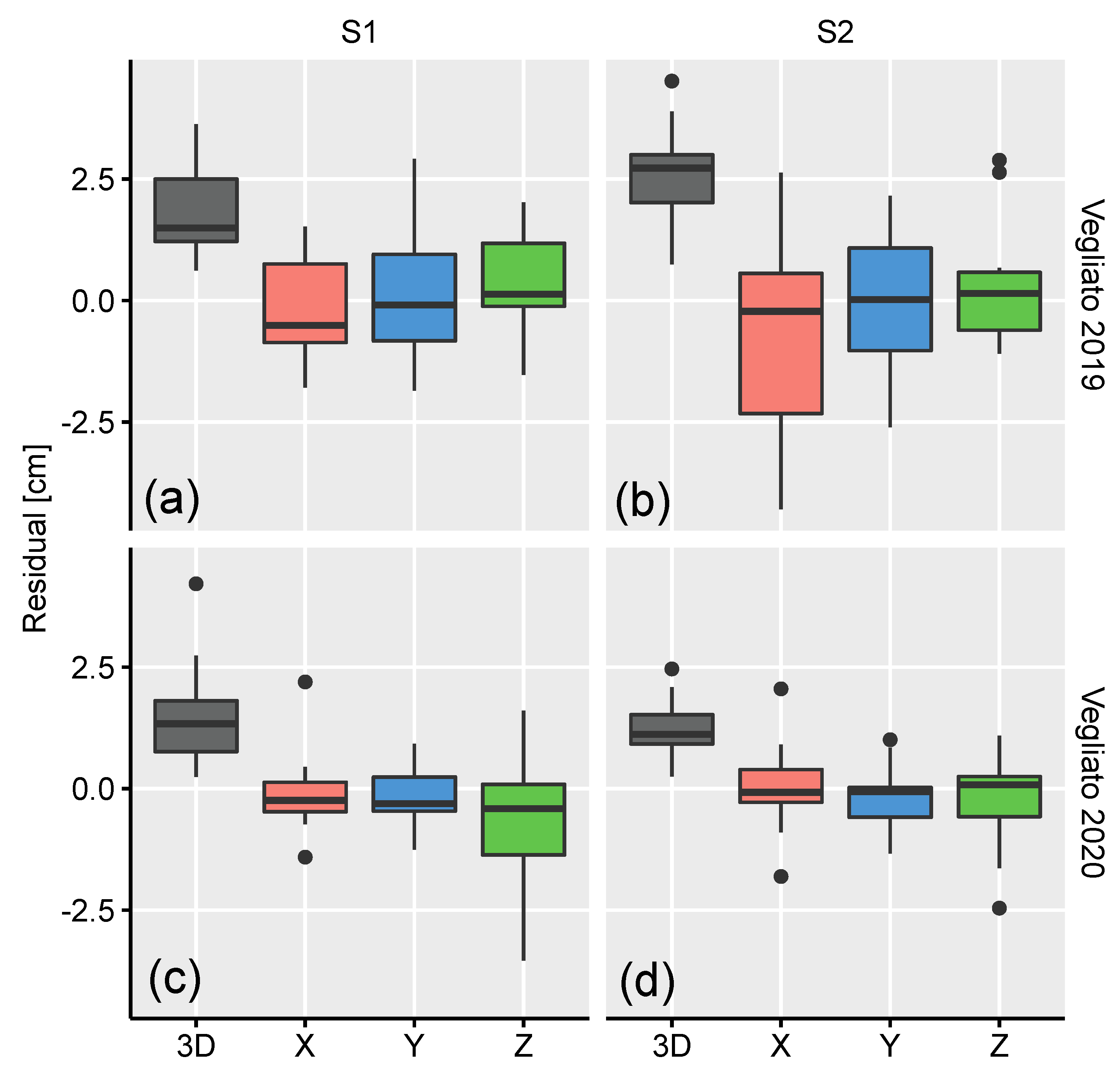
3.1. Assessment of Survey Repeatability and Camera Influence

At first, replicas of the same survey (i.e., performed with the same camera under similar conditions and processed with all available GCPs) are taken into account. As shown by the summary values of Table 4 and further highlighted by the boxplots of the CP residuals reported in Figure 6, for all three study areas datasets acquired with the same equipment lead to equivalent accuracy. For example, for the Palar site the mean 3D error on CPs is 2.1 cm ($\sigma$ = 0.8 cm) for P_S1 and 2.3 ± 0.7 mm for P_S2, respectively, while for the Vegliato area we obtained an average 3D residual of 1.5 ± 1.0 cm for V_S1 and 1.2 ± 0.6 mm for V_S2. Similar behaviour can be appreciated also for the surveys performed with the X5S camera. For instance, the mean absolute error on CPs for the Moscardo area is 1.9 ± 1.2 cm for M_X1 and 1.7 ± 1.1 cm for M_X2. Analogous conclusion can be drawn also considering the residuals expressed as a function of the average GSD: the highest difference can be found between the surveys M_S1 and M_S2, characterized by an average 3D residual on the CPs of 2.2 GSD and 2.8 GSD, respectively.

High coherence between repeated surveys is demonstrated also by the CoDs shown in Figure 3c,f, Figure 4d–f and Figure 5d,f. From the comparisons among dense point clouds, only for the Vegliato study area we notice a mean value of the M3C2 distance that exceeds 1 cm, between V_X1 and V_X2 datasets (−1.7 ± 1.3 cm, see Table 5). In all other cases, repeating the survey with the same camera and using well-distributed GCPs led to average signed distances less than 1 cm and Root Mean Square (RMS) values less than 1.4 cm.

When comparing the results provided by different cameras over the same study area, millimetre differences in terms of average CP residuals can be noticed, except for the Palar study area. In this case, indeed, for the X5S datasets mean and standard deviation are twice the values computed for the Sony image sets. As can be seen from Table 4, the errors grow from 2.1 ± 0.8 cm for P_S1 and 2.3 ± 0.7 cm for P_S2 to 4.0 ± 1.5 cm and 4.0 ± 1.8 cm for the X5S datasets. These discrepancies on CP errors can be noticed also in Figure 6c,d, with the boxplots related to the P_X1 and P_X2 datasets reaching a mean value of 4.0 cm for the 3D residuals, showing high variability both in the $XY$-plane as well as in the altitude component. The lower accuracy that characterises these datasets is revealed also by the average 3D error expressed as a function of the GSD, which reaches 7.7 times the GSD (in the other case studies it is between 2 and 3 times the GSD, see Table 4). To further investigate these outcomes, we divided the CPs according to their location, and computed error statistics for the three subareas considered (Figure 7). The southern region shows greater CP residual values for the X5S datasets, with higher dispersion especially in the Z direction. Analysing the distances between P_S1 and P_X2 point clouds (Figure 3i), instead, it could be noticed that the P_X2 one exhibits a dome-like shape, with positive distances with regard to the P_S1 in the central part of the study sites, and negative values on the boundaries. The RMS for the computed distance is equal to 2.6 cm (Table 5), which represents also the maximum RMS value among all the comparisons made between datasets processed with proper GCP number. These considerations suggest lower accuracy and precision for the P_X1 and P_X2 models.

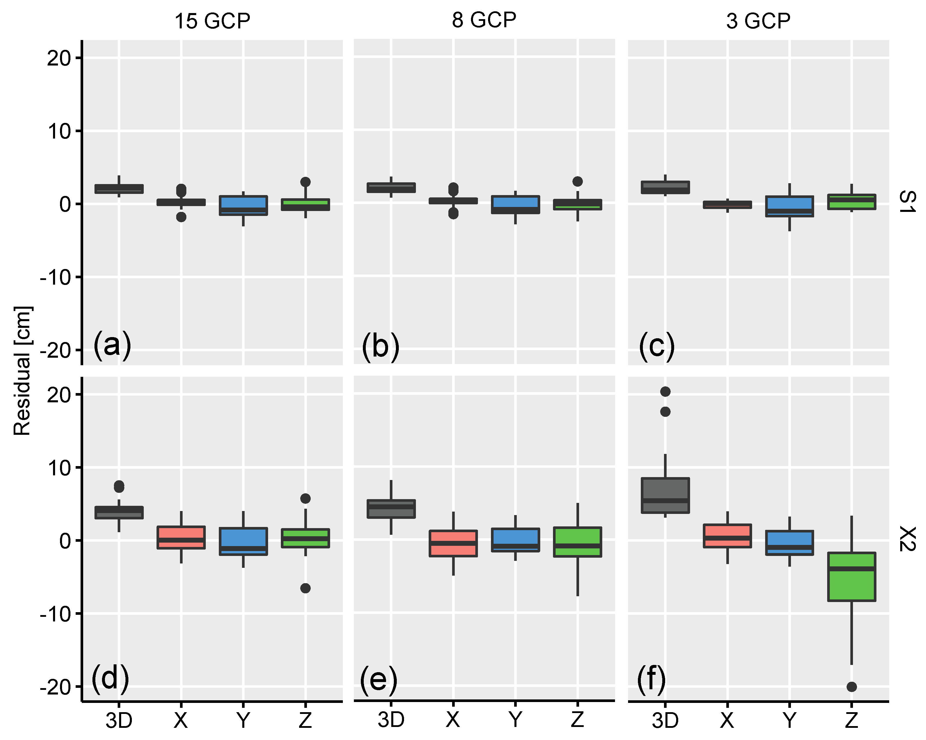
3.2. Assessment of the Effect of the Number and Coordinate Precision of GCPs

As already mentioned in Section 2.2, the influence of the number of GCPs employed in the bundle adjustment was tested in the Palar study site, evaluating the results retrieved with 15, 8 and 3 GCPs. With respect to CP residuals (Figure 8), models generated from the Sony camera dataset show similar behaviour regardless of the number of GCPs, with an average 3D error of 2.1, 2.0 and 2.2 cm for the three cases (15, 8 and 3 GCPs), and a standard deviation of less than 1 cm (see Table 4). Moreover, no significant differences can be noticed in the CoD when comparing the point clouds obtained with 8 GCPs and 15 GCPs (Figure 3d). In fact, the corresponding M3C2 distance is equal to −0.1 ± 0.3 cm, with a RMS of 0.3 cm (Table 5). Analysing the CoD computed from P_S1 and P_S1_3_GCP (Figure 3e), a relative rotation between the two point clouds is slightly visible, which can be due to inaccurate georeferencing of the P_S1_3_GCP model. However, there are still no relevant distances (0.3 ± 0.8 cm on average, RMS is equal to 0.9 cm).

Conversely, GCP density seems to significantly affect the results obtained from the X5S datasets. In the case of 8 GCPs, a small increase in the error affecting all the components can be noticed (from an average 3D residual of 4.0 cm with 15 GCPs to 4.3 cm with 8 GCPs), whereas with only 3 GCPs (that in our case where also not properly distributed) the average residual on the CPs reaches 7.3 ± 5.0 cm, with maximum differences between GNSS and photogrammetric coordinates of 20 cm. Table 4 and Figure 8e also show a large increase of the error in the Z direction, that reaches a mean value of −5.0 cm and a standard deviation of 6.6 cm. The influence of the number of GCPs for the X5S datasets in further highlighted by the comparison between dense point clouds. Figure 3h, in fact, clearly displays decimetre differences (RMS is 10.3 cm) between P_X2 and P_X2_3_GCP, with the model retrieved with only 3 GCPs showing a domed shape. Although to a lesser extent, this behaviour is also visible in the P_X2_8_GCP point cloud. Of course, varying the location and distribution of the 3 GCPs could have significantly changed the results and the error distribution. However, the main goal of this test was to confirm that the minimum number of constraints is usually not sufficient to produce a reliable model.

After having assessed the dependence of the results on the GCP number, it is interesting to verify the influence of the precision of GCP measurements. As explained in Section 2.2, the GNSS coordinates were perturbed adding two different level of Gaussian noise. The consequences are not so relevant: in fact, the 3D residual on the CPs is constant for the three cases (4.0 ± 1.5 cm for P_X2, 4.0 ± 1.6 cm for P_X2_PE1 and 4.0 ± 1.7 cm for P_X2_PE2, see Table 4). Only for the case P_X2_PE2 (Z component perturbed with ${\sigma }_Z=4$ cm) minor distortions in the final model are evident in the form of a dome effect, slightly visible in Figure 3k.

A significant reduction of the model accuracy is instead produced by changing the ‘marker accuracy’ parameter in the bundle adjustment step. We evaluated the results obtained when using the original GCP coordinates but setting this value to 6 cm, noticing also in this case a final model affected by the doming effect. In this situation, the software employs the GCPs as softer constraints, reducing their positive effect on the final bundle adjustment solution.

3.3. Assessment of UAV Flight Mode Impact

To investigate the impact of manual and planned flights, in the Vegliato study area, we compared the results obtained for the Sony datasets acquired with the NT-4C UAV in 2019 and with the DJI Matrice in 2020. The flight missions were performed at the same altitude and using the same camera settings. Focusing on the CPs residuals, one can notice slightly higher 3D error variability for the datasets acquired in manual mode (Figure 9), with mean values of 1.8 ± 0.8 cm and 2.5 ± 1.0 cm (corresponding to 2.7 ± 1.3 GSD and 3.1 ± 1.3 GSD) for V_S1_2019 and V_S2_2019, respectively. The average 3D residual decreases to 1.5 ± 1.0 cm and 1.2 ± 0.6 cm (corresponding to 2.1 ± 1.5 GSD and 1.8 ± 0.9 GSD) for the two image sets collected in planned mode, as shown in Table 4. An indirect comparison can be performed also analyzing the CoDs obtained from the two pairs of flights. In the CoD computed from V_S1_2019 and V_S2_2019 models (Figure 4d) higher distances are visible all over the study area, whereas for the planned flights (Figure 4e) major differences between the two replicas are localised out of the GCP perimeter and downstream of the check dams.

To give further insights on how the flight mode can influence the result, in Figure 10 we show image locations for flights V_S2_2019 (manual flight, Figure 10a) and V_S2 (planned flight, Figure 10b). It is easy to notice the more regular image distribution that characterizes the planned flight, which guarantees uniform overlap and sidelap. Although the average tie-point multiplicity (i.e., the ratio between the total number of projections and the number of tracks) is equivalent for both flight modes (3.94 for the manual and 3.80 for the planned flight), the nonuniform coverage of the area of interest could justify the lower accuracy (see CP residuals, Figure 9) and precision (see the corresponding CoDs, Figure 4d for the manual flights and Figure 4e for the planned mode) that affects the models obtained from manual flights.

4. Discussion

Performing repeated surveys under the same conditions can give an insight on SfM precision. This turns out to be essential when estimating surface changes by means of photogrammetric surveys, in order to avoid false positives or to overestimate changes.

Overall, results reported in Section 3.1 show very good survey repeatability, with minor differences (RMS ≤ 2.1 cm) between the point clouds produced with images acquired with the same camera under similar conditions. Moreover, CoDs do not show spatial patterns that could be ascribed to systematic errors. Most of the analyzed surveys performed on different study areas are characterized by similar accuracy, measured in terms of CP residuals. To avoid biased comparisons due to the different GSD associated to each image set, 3D errors were also expressed as a function of the GSD, resulting in a mean 3D residual ranging from 1.8 to 3.1 times the GSD. The only exception is represented by the surveys carried out with the X5S camera over the Palar site. In these cases, CP errors are slightly higher, reaching an average value of 4.0 ± 1.8 cm for the P_X2 case, that corresponds to 7.7 times the GSD.

This case study also highlights the dependence of the results on the camera used. For the Palar surveys, in fact, models derived from the Sony datasets are more accurate, despite the higher GSD that characterizes these image sets. A possible explanation for such behaviour could be found in the different size of the sensors (357 mm² for the Sony and 225 mm² for the X5S camera, respectively), with the Sony camera producing sharper photos. However, it should also be underlined that the differences between models produced with the two cameras are not so significant for the other sites: the roughness that characterizes the surveyed area can therefore, can play an important role in the final accuracy and precision.

In accordance with the outcomes that can be found in several papers [16,23,29,30], the experiments reported in Section 3.2 clearly demonstrate that another factor that can influence SfM accuracy and precision is the number of GCPs employed in the bundle adjustment. A reliable model, indeed, can be obtained when processing the datasets with proper GCP density and distribution, with GCPs placed also on the boundaries or even outside the study reach [9,31,32]. For the cases previously discussed, using all available GCPs resulted in a density of 5 to 10 GCPs per 100 photos, that respects the suggestion given in [16], according to which more than 3 GCPs per 100 photos should be considered to reach high accuracy. When using a smaller number of GCPs (1.8 GCP per 100 photos in our tests) the model retrieved by the SfM algorithm can reveal local distortions or georeferencing inaccuracies, as shown by P_X2_3_GCP and P_S1_3_GCP, respectively (regardless of the choice of the GCP location). Even for this test, the X5S dataset seems to be more affected by the number of GCPs employed than the Sony images. In particular, the P_X2_3_GCP model shows the well-known dome shape, frequently discussed in the literature [22,33]. The dome effect could have also been mitigated by adding oblique images (20–35° camera angle) or two orthogonal strips [29,34].

We would like to underline that, even in the cases where CP residuals are high and the model presents significant distortion (i.e., P_X2_3_GCP), the reprojection error does not increase (0.76 pixel, see Table 3). As already assessed in other works [20,35], this is a further proof that image-space error is not a reliable indicator of the model accuracy.

The uncertainty and inherent variability of the GNSS measurements, acquired with the PPK technique, do not show a significant impact as demonstrated by the results of the tests performed by perturbing the coordinate of the GCPs. This naturally applies as long as the accuracy of the GCPs is better than or equal to the accuracy of the model.

Finally, regarding the influence of the flight mode, experimental evaluation shows slightly higher accuracy for the model retrieved from planned flights with respect to manual ones (using the same camera for image collection). The former mode, in fact, allows to strictly respect design image overlap and to ensure a more homogeneous coverage of the surveyed area (Figure 10), avoiding that some areas are covered by a few frames, which could negatively affect tie-point visibility and the whole SfM process. Nevertheless, commercial drones without a DEM support can only fly in planned mode at a specific altitude above see level, that causes differences in GSD in steep slope areas.

5. Conclusions

Performing multiple UAV surveys under similar conditions within short time intervals and over several study areas allowed to enhance our understanding of SfM precision. The SfM technique showed high repeatability, whereas significant distances on the resulting 3D model can be appreciated when different cameras are used to survey challenging scenarios (i.e., flat surfaces with homogeneous texture). The SfM reproducibility can therefore be a crucial factor that must be taken into account in change detection applications. When high-precision point cloud data are required, we recommend to test model reproducibility (and in particular the effect of adopting different cameras) over different scenarios, since generalizing the results retrieved over a specific study area could be misleading. GCPs remain essential to generate accurate models, and an independent set of CPs should always be measured to objectively assess the quality of the obtained results.

Geomorphological studies and sediment dynamic analyses require periodic data acquisitions for a considerable time; changing instrumentation (e.g., cameras and GNSS receiver) and protocols (e.g., GCP density or flight mode) during a long evaluation period is thus very likely and it could lead to inconsistent results in data comparison. The method employed in this paper, based on repeated surveys, could be valuable to address these issues.

In a future work, we will investigate how SfM accuracy and precision can affect the volume estimate, computed from multi-temporal surveys over areas characterized by surface changes.

References

1. Singh, A. Review article digital change detection techniques using remotely-sensed data. Int. J. Remote Sens. 1989, 10, 989–1003. [Google Scholar] [CrossRef] [Green Version]
2. Qin, R.; Tian, J.; Reinartz, P. 3D change detection—Approaches and applications. ISPRS J. Photogramm. Remote Sens. 2016, 122, 41–56. [Google Scholar] [CrossRef] [Green Version]
3. Westoby, M.J.; Brasington, J.; Glasser, N.F.; Hambrey, M.J.; Reynolds, J.M. Structure-from-Motion photogrammetry: A low-cost, effective tool for geoscience applications. Geomorphology 2012, 179, 300–314. [Google Scholar] [CrossRef] [Green Version]
4. Carrivick, J.L.; Smith, M.W.; Quincey, D.J. Structure from Motion in the Geosciences; John Wiley & Sons: West Sussex, UK, 2016. [Google Scholar]
5. Turner, D.; Lucieer, A.; De Jong, S.M. Time series analysis of landslide dynamics using an unmanned aerial vehicle (UAV). Remote Sens. 2015, 7, 1736–1757. [Google Scholar] [CrossRef] [Green Version]
6. Gomez, C.; Allouis, T.; Lissak, C.; Hotta, N.; Shinohara, Y.; Hadmoko, D.; Vilimek, V.; Wassmer, P.; Lavigne, F.; Setiawan, A.; et al. High-Resolution Point-Cloud for Landslides in the 21st Century: From Data Acquisition to New Processing Concepts. In Workshop on World Landslide Forum; Springer Nature Switzerland AG: Cham, Switzerland, 2020; pp. 199–213. [Google Scholar]
7. Piermattei, L.; Carturan, L.; Blasi, F.d.; Tarolli, P.; Dalla Fontana, G.; Vettore, A.; Pfeifer, N. Suitability of ground-based SfM–MVS for monitoring glacial and periglacial processes. Earth Surf. Dyn. 2016, 4, 425–443. [Google Scholar] [CrossRef] [Green Version]
8. De Marco, J.; Carturan, L.; Piermattei, L.; Cucchiaro, S.; Moro, D.; Dalla Fontana, G.; Cazorzi, F. Minor Imbalance of the Lowermost Italian Glacier from 2006 to 2019. Water 2020, 12, 2503. [Google Scholar] [CrossRef]
9. Cucchiaro, S.; Cavalli, M.; Vericat, D.; Crema, S.; Llena, M.; Beinat, A.; Marchi, L.; Cazorzi, F. Monitoring topographic changes through 4D-structure-from-motion photogrammetry: Application to a debris-flow channel. Environ. Earth Sci. 2018, 77, 1–21. [Google Scholar] [CrossRef]
10. Backes, D.; Smigaj, M.; Schimka, M.; Zahs, V.; Grznárová, A.; Scaioni, M. River Morphology Monitoring of a Small-Scale Alpine Riverbed Using Drone Photogrammetry and LIDAR. Int. Arch. Photogramm. Remote Sens. Spat. Inf. Sci. 2020, 43, 1017–1024. [Google Scholar] [CrossRef]
11. López, J.B.; Jiménez, G.A.; Romero, M.S.; García, E.A.; Martín, S.F.; Medina, A.L.; Guerrero, J.E. 3D modelling in archaeology: The application of Structure from Motion methods to the study of the megalithic necropolis of Panoria (Granada, Spain). J. Archaeol. Sci. Rep. 2016, 10, 495–506. [Google Scholar] [CrossRef]
12. Cucchiaro, S.; Fallu, D.J.; Zhao, P.; Waddington, C.; Cockcroft, D.; Tarolli, P.; Brown, A.G. SfM photogrammetry for GeoArchaeology. In Developments in Earth Surface Processes; Elsevier: Amsterdam, The Netherlands, 2020; Volume 23, pp. 183–205. [Google Scholar]
13. Eltner, A.; Sofia, G. Structure from motion photogrammetric technique. In Developments in Earth Surface Processes; Elsevier: Amsterdam, The Netherlands, 2020; Volume 23, pp. 1–24. [Google Scholar]
14. Cucchiaro, S.; Maset, E.; Cavalli, M.; Crema, S.; Marchi, L.; Beinat, A.; Cazorzi, F. How does co-registration affect geomorphic change estimates in multi-temporal surveys? GIScience Remote Sens. 2020, 57, 611–632. [Google Scholar] [CrossRef]
15. Fonstad, M.A.; Dietrich, J.T.; Courville, B.C.; Jensen, J.L.; Carbonneau, P.E. Topographic structure from motion: A new development in photogrammetric measurement. Earth Surf. Process. Landf. 2013, 38, 421–430. [Google Scholar] [CrossRef] [Green Version]
16. Sanz-Ablanedo, E.; Chandler, J.H.; Rodríguez-Pérez, J.R.; Ordóñez, C. Accuracy of unmanned aerial vehicle (UAV) and SfM photogrammetry survey as a function of the number and location of ground control points used. Remote Sens. 2018, 10, 1606. [Google Scholar] [CrossRef] [Green Version]
17. Meinen, B.U.; Robinson, D.T. Mapping erosion and deposition in an agricultural landscape: Optimization of UAV image acquisition schemes for SfM-MVS. Remote Sens. Environ. 2020, 239, 111666. [Google Scholar] [CrossRef]
18. Remondino, F.; Nocerino, E.; Toschi, I.; Menna, F. A critical review of automated photogrammetric processing of large datasets. Int. Arch. Photogramm. Remote Sens. Spat. Inf. Sci. 2017, 42, 591–599. [Google Scholar] [CrossRef] [Green Version]
19. Cucchiaro, S.; Maset, E.; Fusiello, A.; Cazorzi, F. 4D-SFM photogrammetry for monitoring sediment dynamics in a debris-flow catchment: Software testing and results comparison. Int. Arch. Photogramm. Remote Sens. Spat. Inf. Sci. 2018, 42, 281–288. [Google Scholar] [CrossRef] [Green Version]
20. Goetz, J.; Brenning, A.; Marcer, M.; Bodin, X. Modeling the precision of structure-from-motion multi-view stereo digital elevation models from repeated close-range aerial surveys. Remote Sens. Environ. 2018, 210, 208–216. [Google Scholar] [CrossRef]
21. James, M.R.; Robson, S.; Smith, M.W. 3-D uncertainty-based topographic change detection with structure-from-motion photogrammetry: Precision maps for ground control and directly georeferenced surveys. Earth Surf. Process. Landf. 2017, 42, 1769–1788. [Google Scholar] [CrossRef]
22. James, M.R.; Antoniazza, G.; Robson, S.; Lane, S.N. Mitigating systematic error in topographic models for geomorphic change detection: Accuracy, precision and considerations beyond off-nadir imagery. Earth Surf. Process. Landf. 2020, 45, 2251–2271. [Google Scholar] [CrossRef]
23. Clapuyt, F.; Vanacker, V.; Van Oost, K. Reproducibility of UAV-based earth topography reconstructions based on Structure-from-Motion algorithms. Geomorphology 2016, 260, 4–15. [Google Scholar] [CrossRef]
24. Bartlett, J.; Frost, C. Reliability, repeatability and reproducibility: Analysis of measurement errors in continuous variables. Ultrasound Obstet. Gynecol. Off. J. Int. Soc. Ultrasound Obstet. Gynecol. 2008, 31, 466–475. [Google Scholar] [CrossRef] [PubMed]
25. James, M.R.; Robson, S.; d’Oleire Oltmanns, S.; Niethammer, U. Optimising UAV topographic surveys processed with structure-from-motion: Ground control quality, quantity and bundle adjustment. Geomorphology 2017, 280, 51–66. [Google Scholar] [CrossRef] [Green Version]
26. Marchi, L.; Cazorzi, F.; Arattano, M.; Cucchiaro, S.; Cavalli, M.; Crema, S. Debris flows recorded in the Moscardo catchment (Italian Alps) between 1990 and 2019. Nat. Hazards Earth Syst. Sci. 2021, 21, 87–97. [Google Scholar] [CrossRef]
27. Piermattei, L.; Carturan, L.; Guarnieri, A. Use of terrestrial photogrammetry based on structure-from-motion for mass balance estimation of a small glacier in the Italian alps. Earth Surf. Process. Landf. 2015, 40, 1791–1802. [Google Scholar] [CrossRef]
28. Lague, D.; Brodu, N.; Leroux, J. Accurate 3D comparison of complex topography with terrestrial laser scanner: Application to the Rangitikei canyon (NZ). ISPRS J. Photogramm. Remote Sens. 2013, 82, 10–26. [Google Scholar] [CrossRef] [Green Version]
29. Manfreda, S.; Dvorak, P.; Mullerova, J.; Herban, S.; Vuono, P.; Arranz Justel, J.J.; Perks, M. Assessing the Accuracy of Digital Surface Models Derived from Optical Imagery Acquired with Unmanned Aerial Systems. Drones 2019, 3, 15. [Google Scholar] [CrossRef] [Green Version]
30. Oniga, V.E.; Breaban, A.I.; Pfeifer, N.; Chirila, C. Determining the suitable number of ground control points for UAS images georeferencing by varying number and spatial distribution. Remote Sens. 2020, 12, 876. [Google Scholar] [CrossRef] [Green Version]
31. James, M.R.; Robson, S. Straightforward reconstruction of 3D surfaces and topography with a camera: Accuracy and geoscience application. J. Geophys. Res. Earth Surf. 2012, 117. [Google Scholar] [CrossRef] [Green Version]
32. Eltner, A.; Kaiser, A.; Castillo, C.; Rock, G.; Neugirg, F.; Abellán, A. Image-based surface reconstruction in geomorphometry—merits, limits and developments. Earth Surf. Dyn. 2016, 4, 359–389. [Google Scholar] [CrossRef] [Green Version]
33. James, M.R.; Robson, S. Mitigating systematic error in topographic models derived from UAV and ground-based image networks. Earth Surf. Process. Landf. 2014, 39, 1413–1420. [Google Scholar] [CrossRef] [Green Version]
34. Nesbit, P.R.; Hugenholtz, C.H. Enhancing UAV–SfM 3D Model Accuracy in High-Relief Landscapes by Incorporating Oblique Images. Remote Sens. 2019, 11, 239. [Google Scholar] [CrossRef] [Green Version]
35. Maset, E.; Magri, L.; Toschi, I.; Fusiello, A. Bundle Block Adjustment with Constrained Relative Orientations. ISPRS Ann. Photogramm. Remote Sens. Spat. Inf. Sci. 2020, 2, 49–55. [Google Scholar] [CrossRef]
Figure 1. (a,b) Geographic location of the study areas, (c,d) Palar study area and a detail of the grain size in the riverbed, (e,f) Vegliato area and a portion of the fluvial terraces, (g,h) Moscardo site and a detail of the heterogeneous granulomerty in the channel reach.
Remotesensing 13 02572 g001
Figure 2. Comparisons performed for the three study areas between consecutive surveys to test survey repeatability (1), different cameras (2), various number of GCPs employed in the bundle adjustment (3), different 3D coordinate precision of GCPs (4) and two flight modes (5). The comparisons are labelled according to the names of the used datasets. The dataset characteristics are reported in Table 2.
Remotesensing 13 02572 g002
Figure 3. CoDs of Palar models obtained using different cameras, different number of GCPs and varying GCP coordinate precision. (a) Study area. (b) GCPs (red) and CPs (green) positions. (c,f,i) CoDs derived from Sony and X5S point clouds, exploiting all available GCPs in the bundle adjustment. Comparisons between the reference point cloud and those obtained with 8 and 3 GCPs are reported in (d,e) for Sony image set and (g,h) for X5S camera. In (j,k) the effect of two levels of perturbation error introduced in the GCP coordinates are shown for X5S camera. Distance values are pictured with a red-to-blue gradient.
Remotesensing 13 02572 g003
Figure 4. CoDs of Vegliato datasets collected in different years using different cameras. (a) Study area. (b,c) GCPs (red) and CPs (green) positions for 2019 and 2020 surveys. (d,e) CoDs derived from Sony datasets for 2019 and 2020, respectively, and (f) the one from X5S. The CoD in (g) represents the comparison between the point clouds derived from different cameras (V_S1 vs V_X2). Distance values are pictured with a red-to-blue gradient.
Remotesensing 13 02572 g004
Figure 5. CoDs of Moscardo models. Evaluated datasets were collected in different years using different cameras. (a) Study area (water have been removed to avoid biased comparisons). (b,c) GCPs (red) and CPs (green) positions for 2019 and 2020 surveys. (d) CoD derived from the comparison between M_S1 and M_S2. (f) CoD computed between X5S surveys (M_X1 vs M_X2). Distance values are pictured with a red-to-blue gradient.
Remotesensing 13 02572 g005
Figure 6. Comparison of CP residuals obtained from different surveys and study areas. (ad) Palar, (eh) Vegliato 2020, (il) Moscardo. ‘S’ were surveys performed with the Sony camera, whereas ‘X’ referes to X5S datasets. The 3D total error is reported in grey, while pink, blue and green represents residuals in the X, Y and Z direction, respectively. These results were obtained using all available GCPs for each study area.
Remotesensing 13 02572 g006
Figure 7. Comparison of CPs residuals for Palar study area. Statistics are computed diving the CPs according to their location (Figure 3b) into three areas: (ad) North boundary (including check points P02, P06, P05, P09 and P18), (eh) Center (P08, P10, P12, P16, P14 and P21) and (il) South boundary (P23, P24, P27, P29, P30 and P33). ‘S’ surveys were performed with the Sony camera, whereas ‘X’ refers to X5S datasets. The 3D total error is reported in gray, while pink, blue and green represents residuals in the X, Y and Z direction, respectively. These results were obtained using all available GCPs.
Remotesensing 13 02572 g007
Figure 8. Comparison of CPs residuals for Palar study area using different cameras and different number of GCPs (3, 8 and 15 GCPs). ‘S’ surveys were performed with the Sony camera (ac), whereas ‘X’ refers to X5S datasets (df). The 3D total error is reported in grey, while pink, blue and green represents residuals in the X, Y and Z direction, respectively.
Remotesensing 13 02572 g008
Figure 9. Comparison of CPs residuals for Vegliato study area using manual (a,b) or programmed (c,d) flight mode. Sony camera was employed for data acquisitions. The 3D total error is reported in gray, while pink, blue and green represents residuals in the X, Y and Z direction, respectively.
Remotesensing 13 02572 g009
Figure 10. Image locations for flights (a) V_S2_2019 (manual flight) and (b)V_S2 (planned flight). Please note the more regular image distribution that characterizes the planned flight.
Remotesensing 13 02572 g010