
Integrating Aerial LiDAR and Very-High-Resolution Images for Urban Functional Zone Mapping


Abstract
:
1. Introduction
- To integrate multi-machine learning algorithms and various features, primarily 3D USPs, for enhancing land cover mapping;
- To perform UFZ mapping by coupling 3D USPs and multi-classifiers (MLCs);
- To evaluate the influence of 3D USPs on the classifications of both land covers and UFZs.
2. Study Area and Data
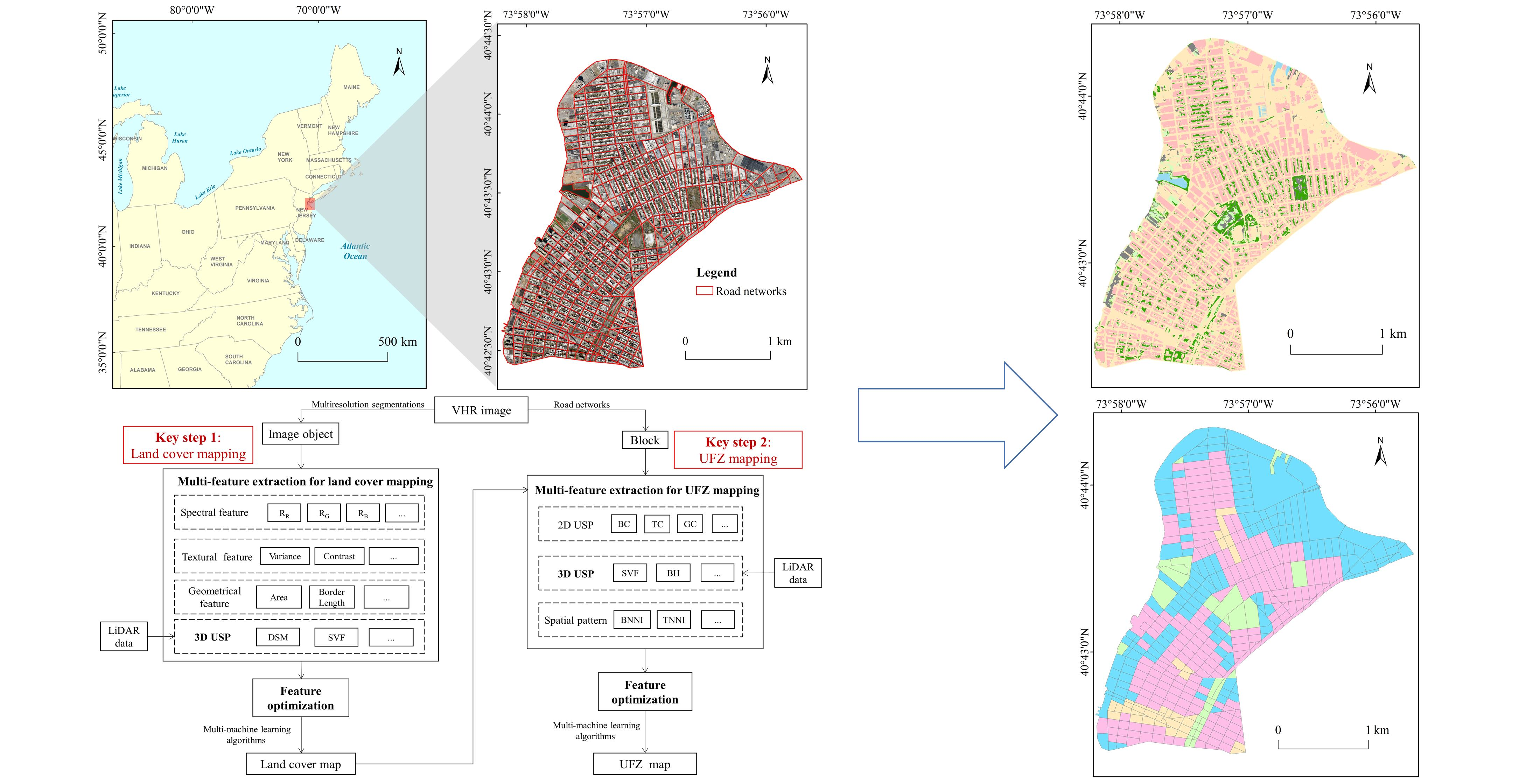
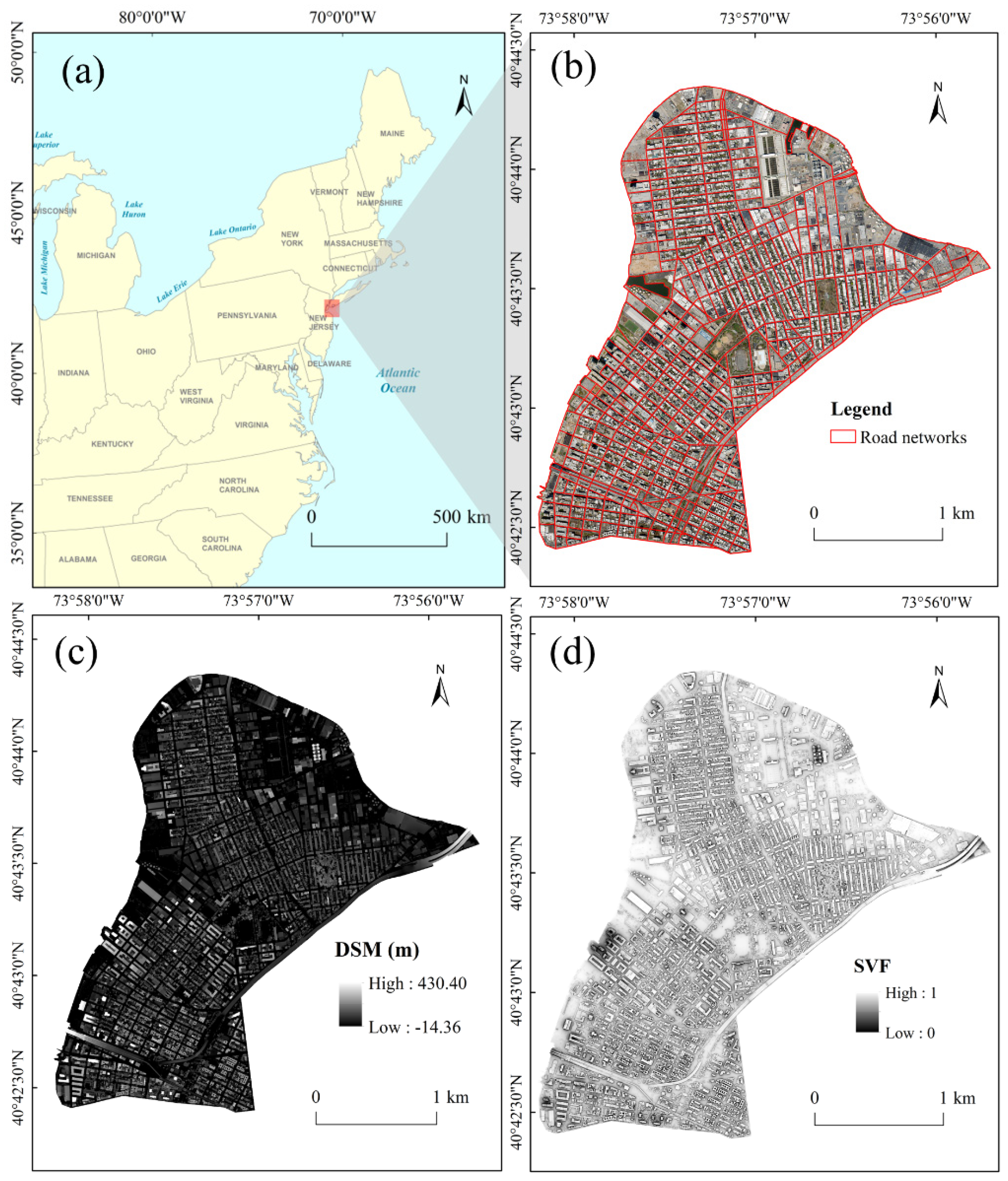
2.1. Study Area
2.2. Data
- VHR images
- LiDAR point clouds
- Road networks and land-lot information
3. Methods
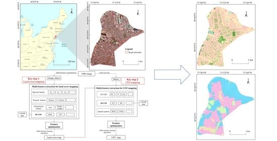
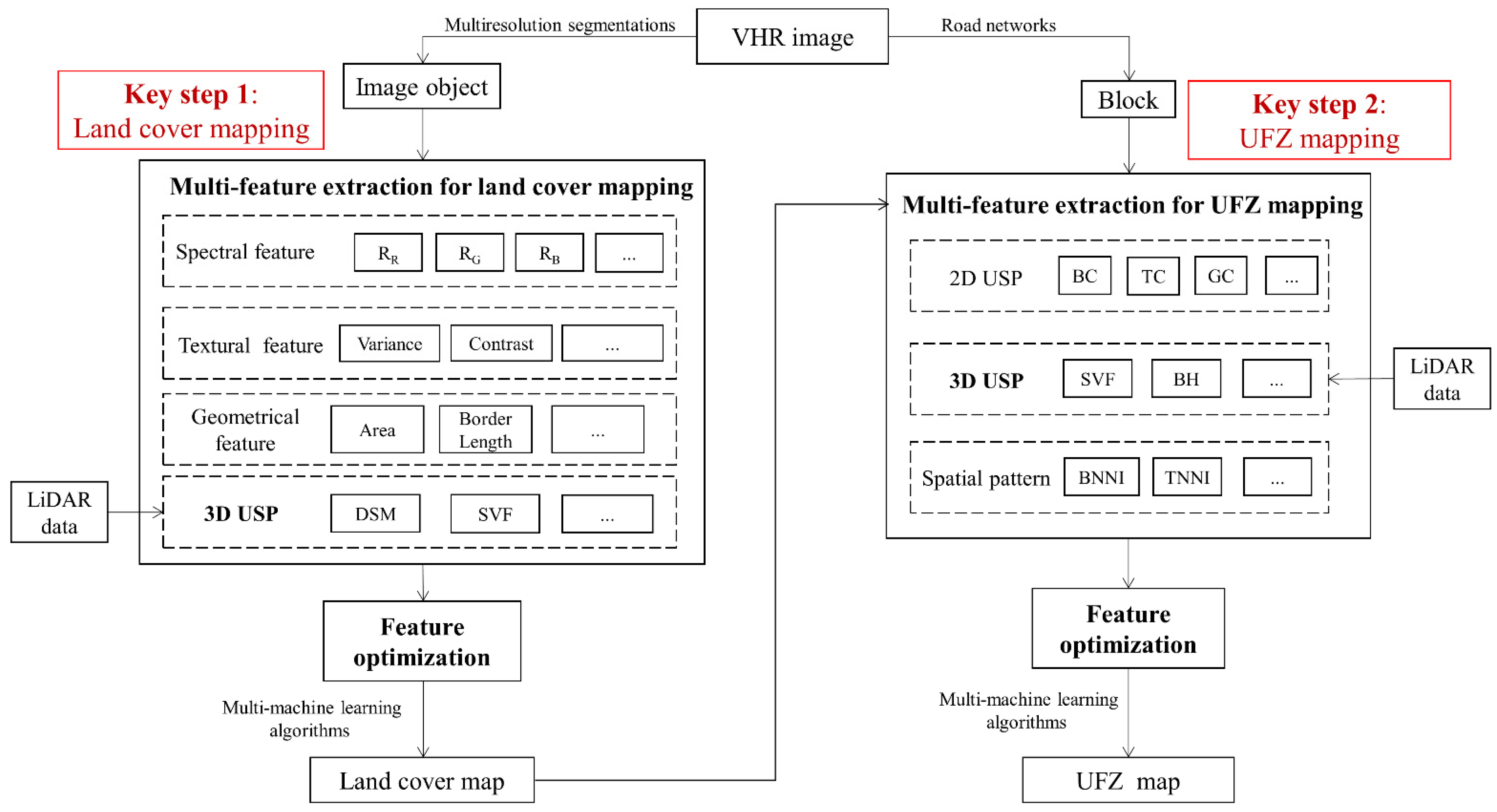
3.1. Overview of the Study Approach
3.2. Land Cover Mapping
3.2.1. Multi-Feature Extraction
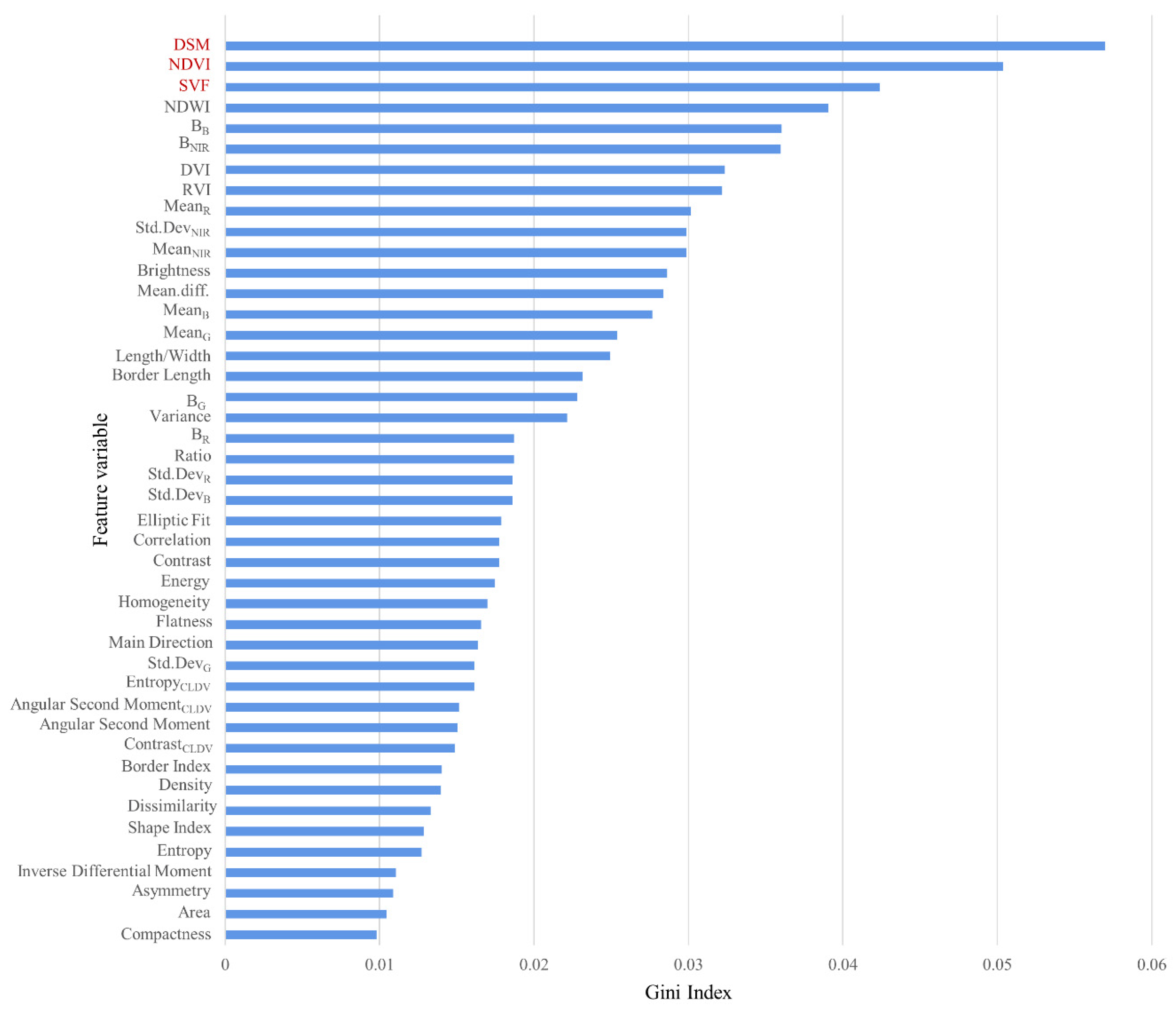
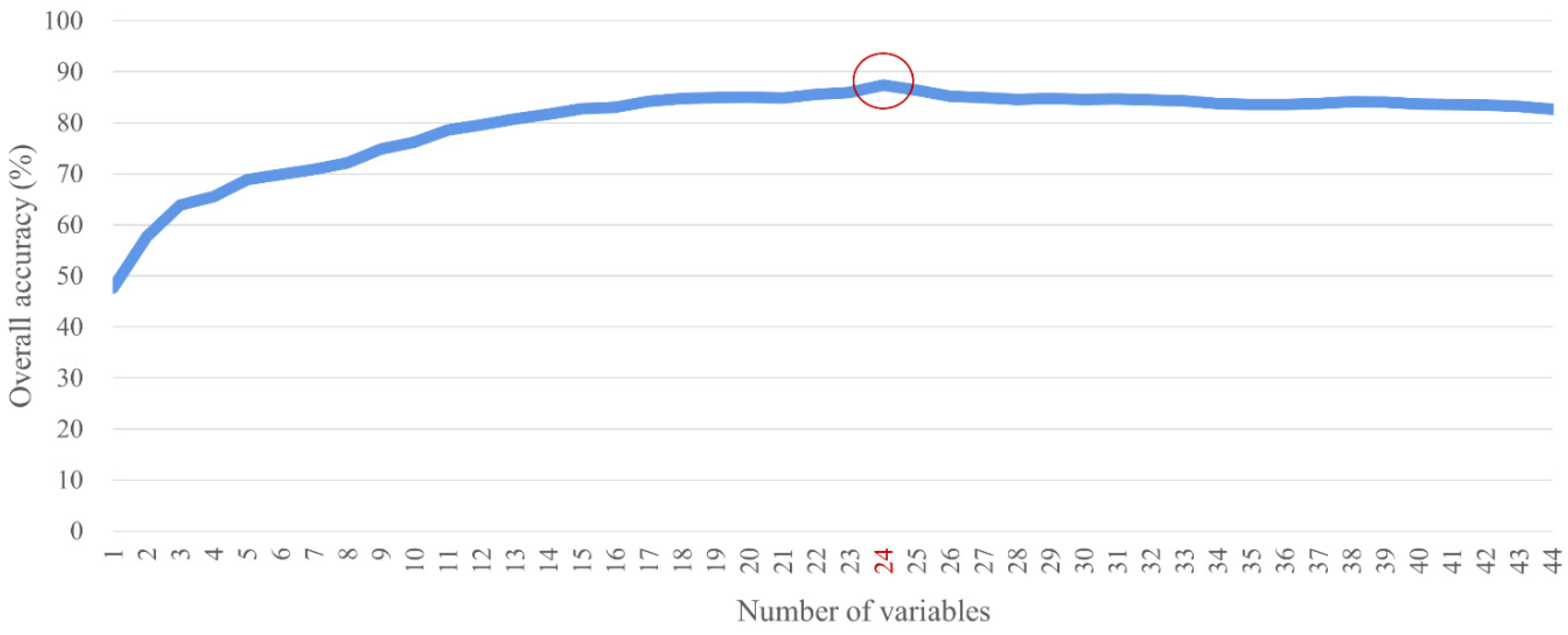
3.2.2. Feature Optimization
3.2.3. The Classifier of Multiple Machine Learning
- (1)
- RF classifier consists of multiple decision trees and can utilize different trees to train samples and predict results. In particular, each tree would yield its predicted result. Then, by counting the vote results in different decision trees, RF integrates their vote results to predict the final results. Therefore, the RF model can significantly improve the classification results compared with a single decision tree. In addition, RF has a good performance for the outlier as well as noise and can effectively avoid overfitting [3,49].
- (2)
- KNN classifier measures the weight of its neighbors when performs a new instance. The classifier labeled objects with different categories according to the weight and is more suitable than other classifiers when the class fields overlaps in the sample set [50].
- (3)
- LDA classifier projects the training sample on a straight line to make project objects of the same class as close as possible; in contrast, heterogeneous sample projection points away from as far as possible. The classifier assumes that all data sets are followed by a normal distribution and can reduce the dimensions of the original data. LDA classifier calculates the probability density of each class sample, and the classification results depend on the maximum probability of each category [51,52].
3.2.4. Classification Post-Processing and Accuracy Evaluation
3.3. UFZ Mapping
3.3.1. Feature Extraction
3.3.2. Experiment Design
4. Results
4.1. Urban Land Cover Mapping
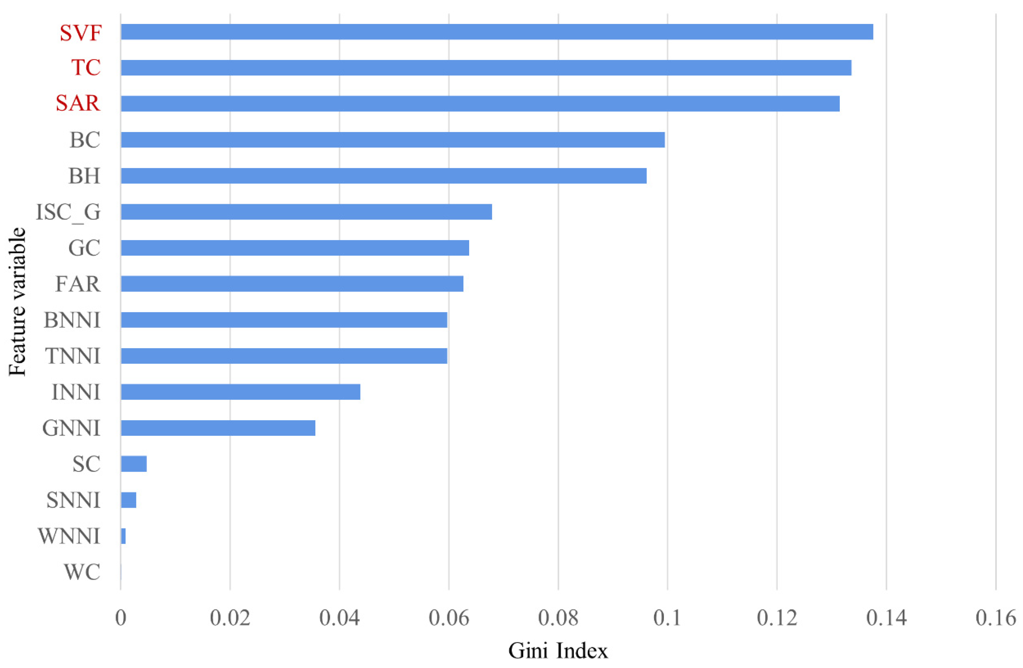
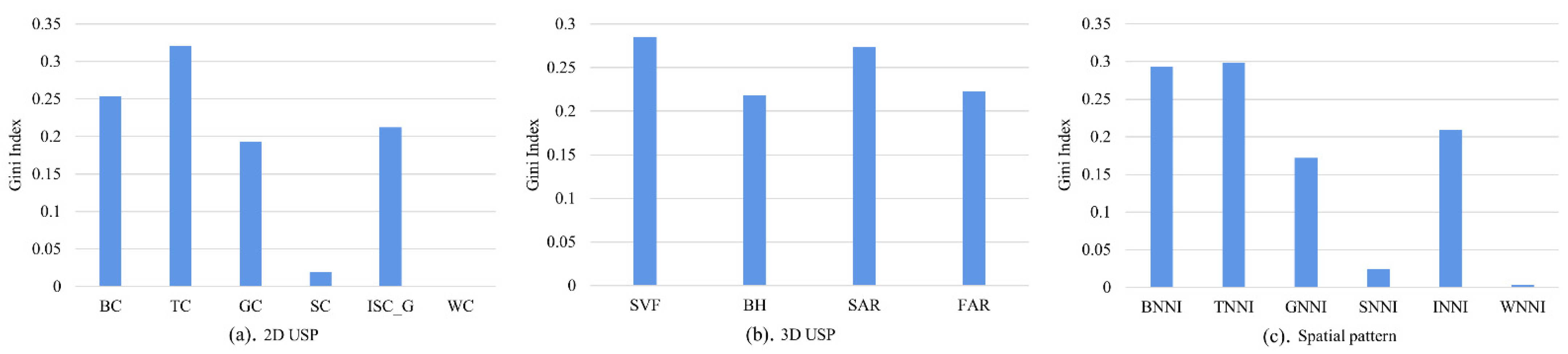
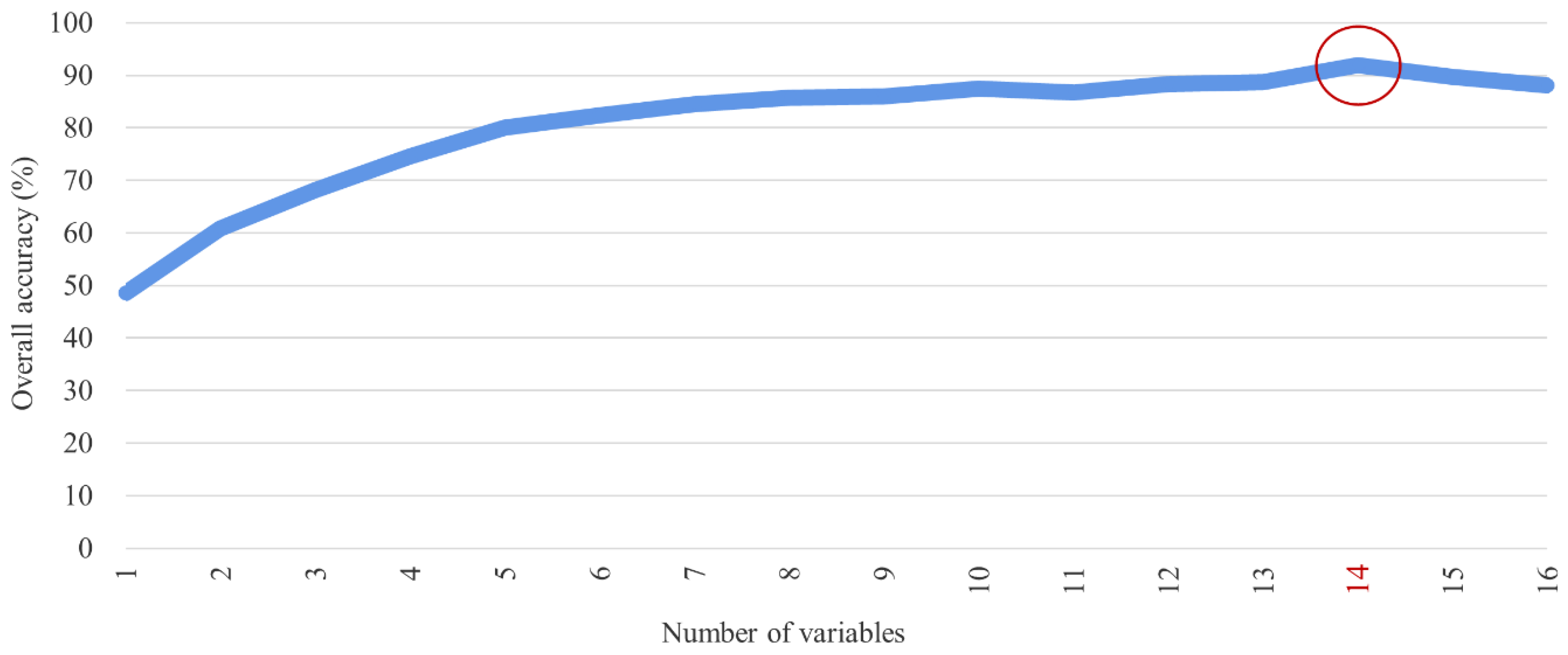
4.1.1. Results of Feature Optimization
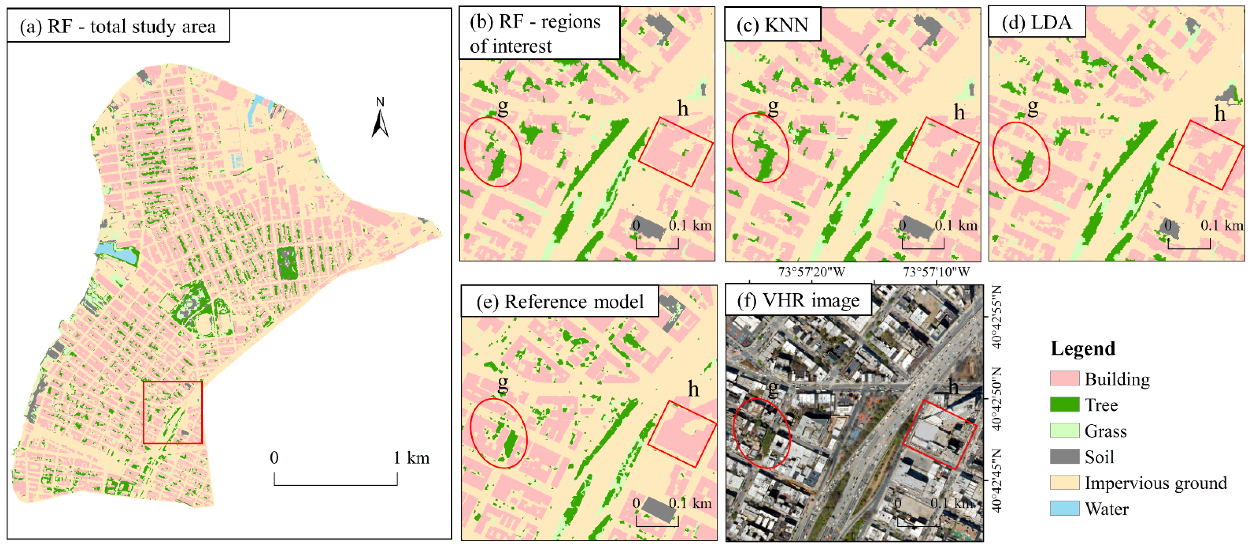
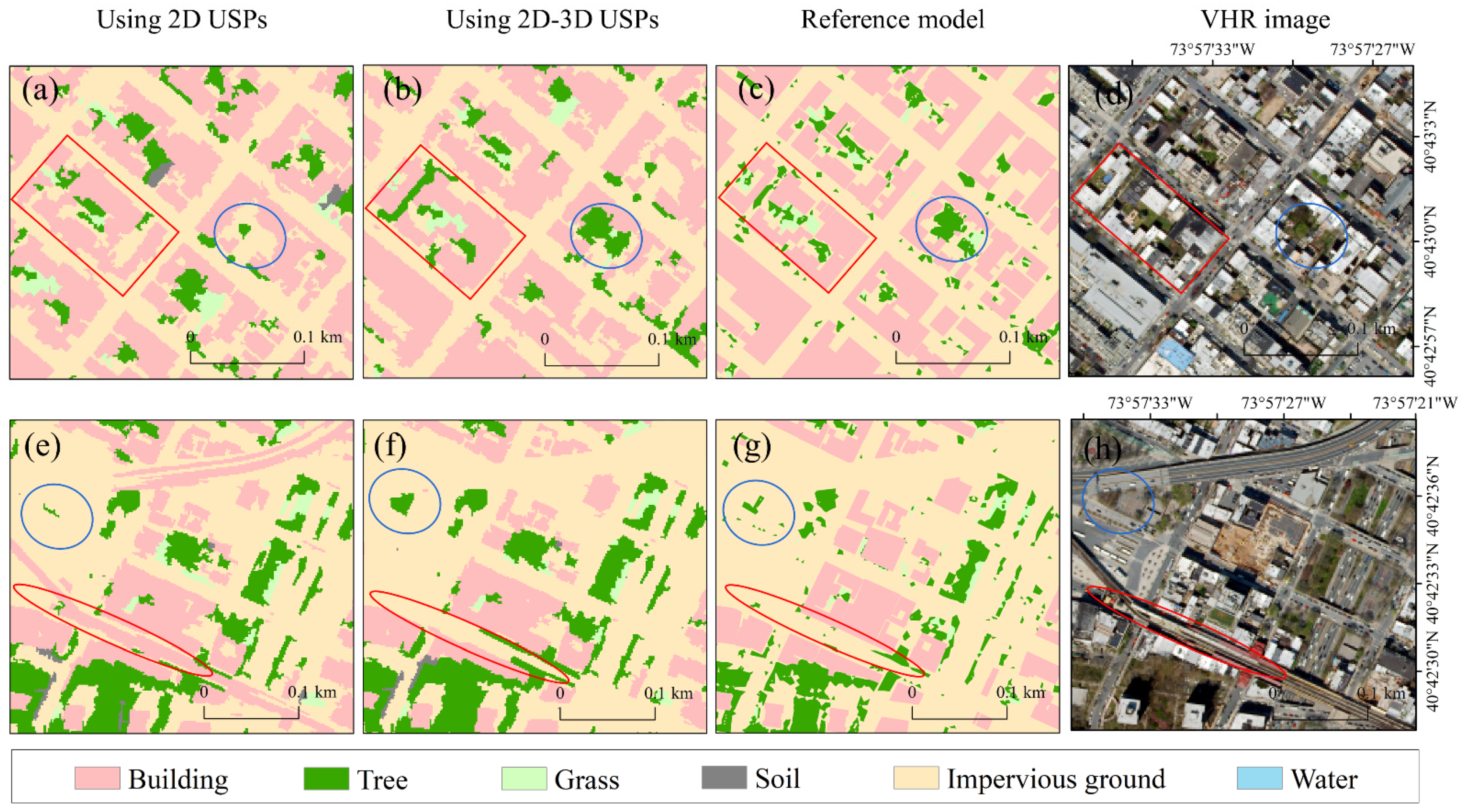
4.1.2. Results of Land Cover Mapping
4.1.3. Advantages of Using 3D USPs to Land-Cover Mapping
4.2. UFZ Mapping
4.2.1. Results of Feature Optimization
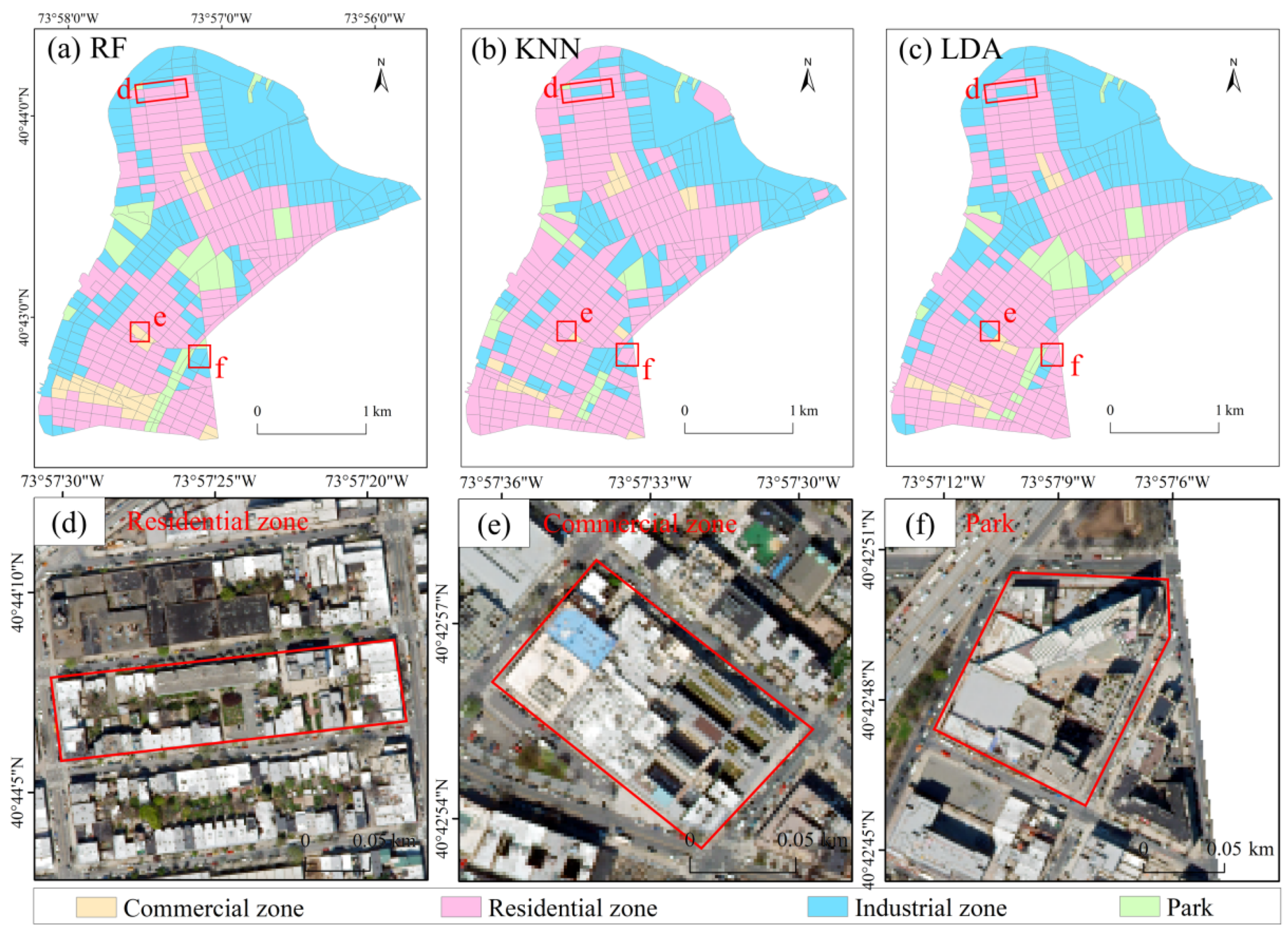
4.2.2. Results of UFZ Mapping
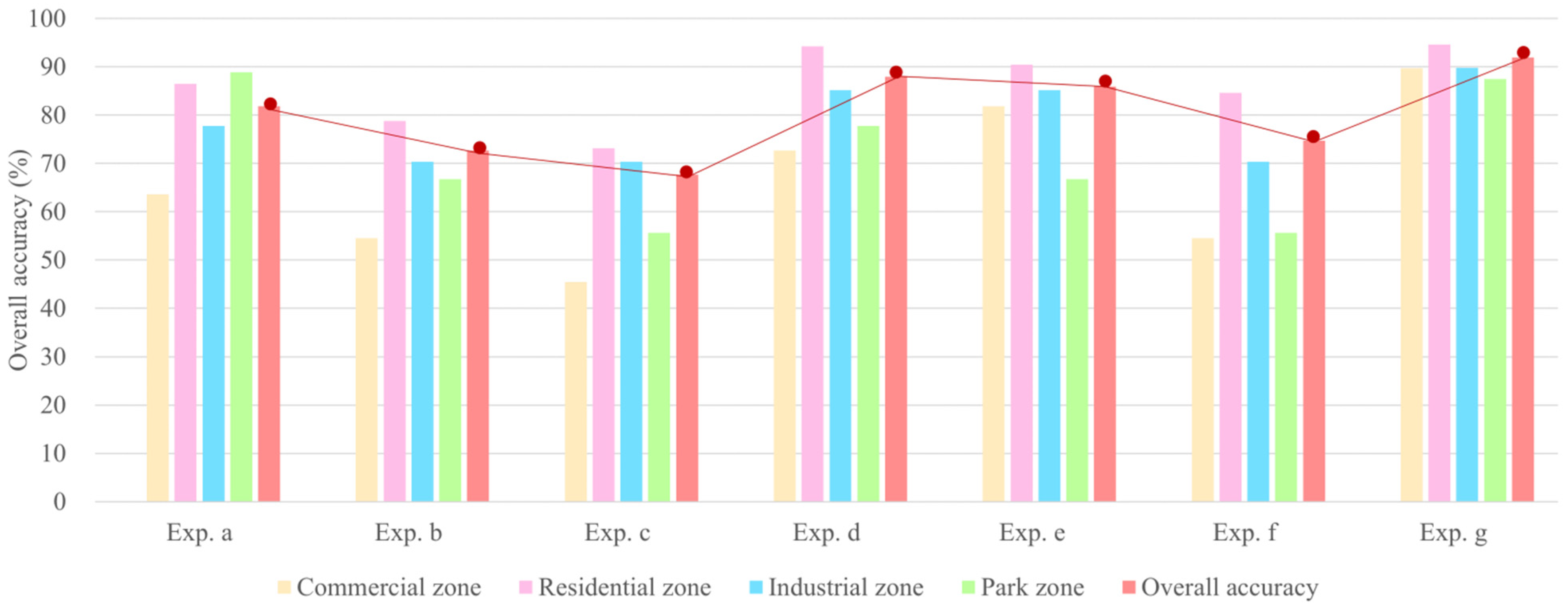
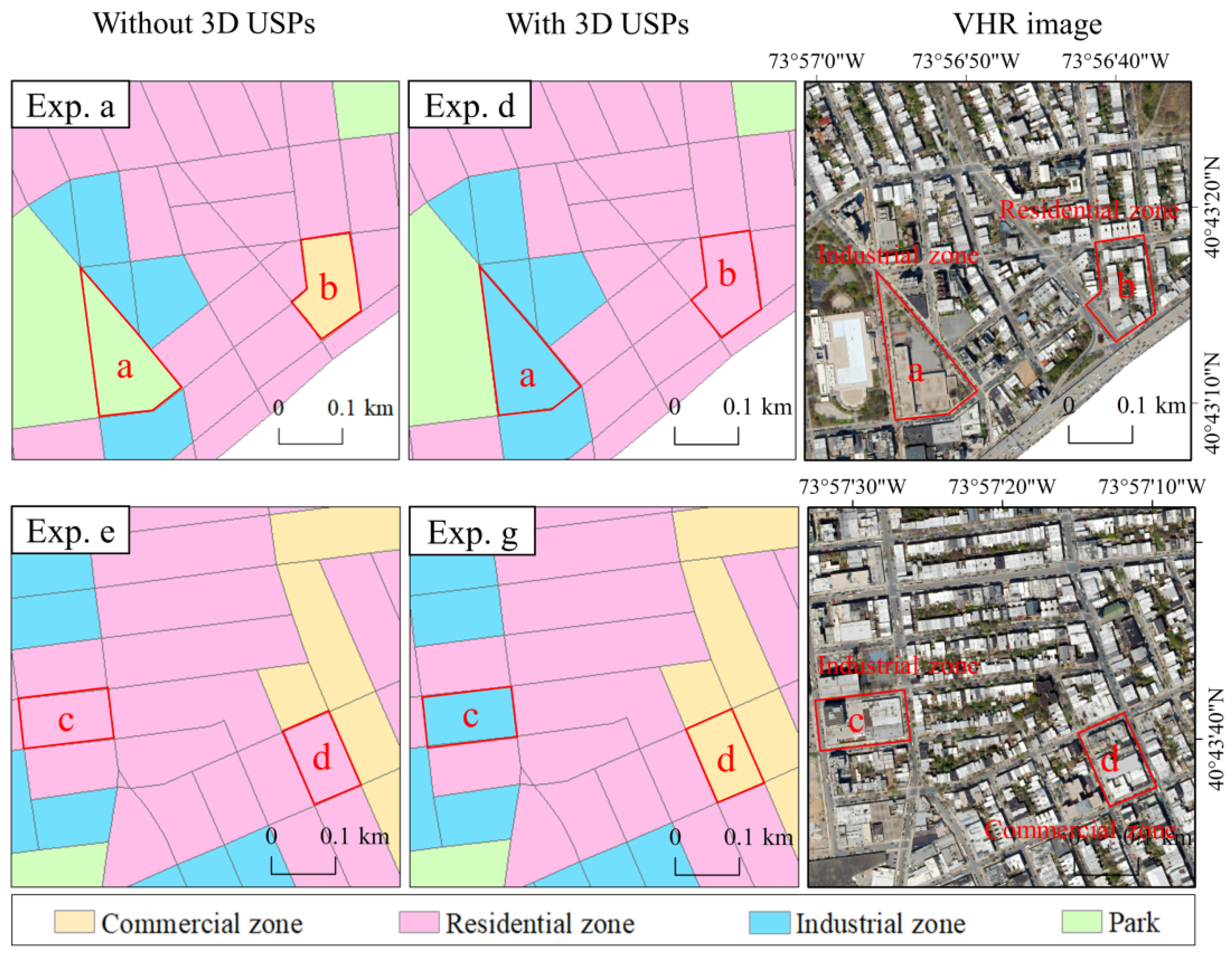
4.2.3. Advantages of Using 3D USPs to UFZ Mapping
5. Discussion
6. Conclusions
Supplementary Materials
Author Contributions
Funding
Institutional Review Board Statement
Informed Consent Statement
Data Availability Statement
Conflicts of Interest
References
- Zhang, X.; Du, S.; Wang, Q. Integrating bottom-up classification and top-down feedback for improving urban land-cover and functional-zone mapping. Remote Sens. Environ. 2018, 212, 231–248. [Google Scholar] [CrossRef]
- Alberti, M.; Weeks, R.; Coe, S. Urban land-cover change analysis in central puget sound. Photogramm. Eng. Remote Sens. 2004, 70, 1043–1052. [Google Scholar] [CrossRef] [Green Version]
- Yao, Y.; Li, X.; Liu, X.; Liu, P.; Liang, Z.; Zhang, J.; Mai, K. Sensing spatial distribution of urban land use by integrating points-of-interest and Google Word2Vec model. Int. J. Geogr. Inf. Sci. 2017, 31, 825–848. [Google Scholar] [CrossRef]
- Kane, K.; Tuccillo, J.; York, A.M.; Gentile, L.; Ouyang, Y. A spatio-temporal view of historical growth in Phoenix, Arizona, USA. Landsc. Urban Plan. 2014, 121, 70–80. [Google Scholar] [CrossRef]
- Zhou, G.; Li, C.; Li, M.; Zhang, J.; Liu, Y. Agglomeration and diffusion of urban functions: An approach based on urban land use conversion. Habitat Int. 2016, 56, 20–30. [Google Scholar] [CrossRef]
- Heiden, U.; Heldens, W.; Roessner, S.; Segl, K.; Esch, T.; Mueller, A. Urban structure type characterization using hyperspectral remote sensing and height information. Landsc. Urban Plan. 2012, 105, 361–375. [Google Scholar] [CrossRef]
- Hu, S.; Wang, L. Automated urban land-use classification with remote sensing. Int. J. Remote Sens. 2012, 34, 790–803. [Google Scholar] [CrossRef]
- Feng, Y.; Du, S.; Myint, S.W.; Shu, M. Do urban functional zones affect land surface temperature differently? A case study of Beijing, China. Remote Sens. 2019, 11, 1802. [Google Scholar] [CrossRef] [Green Version]
- Zhang, X.; Du, S.; Zheng, Z. Heuristic sample learning for complex urban scenes: Application to urban functional-zone mapping with VHR images and POI data. ISPRS J. Photogramm. Remote Sens. 2020, 161, 1–12. [Google Scholar] [CrossRef]
- Xiao, J.; Shen, Y.; Ge, J.; Tateishi, R.; Tang, C.; Liang, Y.; Huang, Z. Evaluating urban expansion and land use change in Shijiazhuang, China, by using GIS and remote sensing. Landsc. Urban Plan. 2006, 75, 69–80. [Google Scholar] [CrossRef]
- Zhang, X.; Du, S.; Wang, Q. Hierarchical semantic cognition for urban functional zones with VHR satellite images and POI data. ISPRS J. Photogramm. Remote Sens. 2017, 132, 170–184. [Google Scholar] [CrossRef]
- Hu, T.; Yang, J.; Li, X.; Gong, P. Mapping urban land use by using landsat images and open social data. Remote Sens. 2016, 8, 151. [Google Scholar] [CrossRef]
- Zhou, W.; Ming, D.; Lv, X.; Zhou, K.; Bao, H.; Hong, Z. SO–CNN based urban functional zone fine division with VHR remote sensing image. Remote Sens. Environ. 2020, 236, 111458. [Google Scholar] [CrossRef]
- Cao, S.; Weng, Q.; Du, M.; Li, B.; Zhong, R.; Mo, Y. Multi-scale three-dimensional detection of urban buildings using aerial LiDAR data. GISci. Remote Sens. 2020, 57, 1125–1143. [Google Scholar] [CrossRef]
- Liu, C.; Huang, X.; Zhu, Z.; Chen, H.; Tang, X.; Gong, J. Automatic extraction of built-up area from ZY3 multi-view satellite imagery: Analysis of 45 global cities. Remote Sens. Environ. 2019, 226, 51–73. [Google Scholar] [CrossRef]
- Huang, X.; Chen, H.; Gong, J. Angular difference feature extraction for urban scene classification using ZY-3 multi-angle high-resolution satellite imagery. ISPRS J. Photogramm. Remote Sens. 2018, 135, 127–141. [Google Scholar] [CrossRef]
- New York City Office of Information Technology Services (NYITS). High-Resolution Orthophotos of Red, Green, Blue, and Near-Infrared Bands. Available online: http://gis.ny.gov/gateway/mg/metadata.cfm (accessed on 1 February 2020).
- New York City Department of Information Technology and Telecommunications (NYCDITT). 2017 ALS Data. Available online: http://gis.ny.gov/elevation/lidar-coverage.htm (accessed on 1 February 2019).
- Shin, H.B. Residential redevelopment and the entrepreneurial local state: The implications of Beijing’s shifting emphasis on urban redevelopment policies. Urban Stud. 2009, 46, 2815–2839. [Google Scholar] [CrossRef] [Green Version]
- Zhao, P.; Lu, B. Transportation implications of metropolitan spatial planning in mega-city Beijing. Int. Dev. Plan. Rev. 2009, 31, 235–261. [Google Scholar] [CrossRef]
- Benz, U.C.; Hofmann, P.; Willhauck, G.; Lingenfelder, I.; Heynen, M. Multi-resolution, object-oriented fuzzy analysis of remote sensing data for GIS-ready information. ISPRS J. Photogramm. Remote Sens. 2004, 58, 239–258. [Google Scholar] [CrossRef]
- Baatz, M.; Schape, A. Multiresolution segmentation: An optimization approach for high quality multi-scale image segmentation. Angew. Geogr. Inf. Verarbeitung. 2000, 12, 12–23. [Google Scholar]
- Burnett, C.; Blaschke, T. A multi-scale segmentation/object relationship modelling methodology for landscape analysis. Ecol. Model. 2003, 168, 233–249. [Google Scholar] [CrossRef]
- Hay, G.J.; Blaschke, T.; Marceau, D.J.; Bouchard, A. A comparison of three image-object methods for the multiscale analysis of landscape structure. ISPRS J. Photogramm. Remote Sens. 2003, 57, 327–345. [Google Scholar] [CrossRef]
- Silveira, M.; Nascimento, J.; Marques, J.S.; Marcal, A.R.S.; Mendonca, T.; Yamauchi, S.; Maeda, J.; Rozeira, J. Comparison of segmentation methods for melanoma diagnosis in dermoscopy images. IEEE J. Sel. Top. Signal Process. 2009, 3, 35–45. [Google Scholar] [CrossRef]
- Drǎguţ, L.; Tiede, D.; Levick, S. ESP: A tool to estimate scale parameter for multiresolution image segmentation of remotely sensed data. Int. J. Geogr. Inf. Sci. 2010, 24, 859–871. [Google Scholar] [CrossRef]
- Peña-Barragán, J.M.; Ngugi, M.K.; Plant, R.E.; Six, J. Object-based crop identification using multiple vegetation indices, textural features and crop phenology. Remote Sens. Environ. 2011, 115, 1301–1316. [Google Scholar] [CrossRef]
- Cleve, C.; Kelly, M.; Kearns, F.R.; Moritz, M. Classification of the wildland–urban interface: A comparison of pixel- and object-based classifications using high-resolution aerial photography. Comput. Environ. Urban Syst. 2008, 32, 317–326. [Google Scholar] [CrossRef]
- Faridatul, M.I.; Wu, B. Automatic classification of major urban land covers based on novel spectral indices. ISPRS Int. J. Geo-Inf. 2018, 7, 453. [Google Scholar] [CrossRef] [Green Version]
- Jiang, Z.; Huete, A.R.; Chen, J.; Chen, Y.; Li, J.; Yan, G.; Zhang, X. Analysis of NDVI and scaled difference vegetation index retrievals of vegetation fraction. Remote Sens. Environ. 2006, 101, 366–378. [Google Scholar] [CrossRef]
- Person, R.L.; Miller, L.D. Remote mapping of standing crop biomass for estimation of the productivity of the short-grass prairie. In Proceedings of the Eighth International Symposium on Remote Sensing of Environment, Ann Arbor, MI, USA, 2–6 October 1972; Volume 2, pp. 1357–1381. [Google Scholar]
- Tucker, C.J. Red and photographic infrared linear combinations for monitoring vegetation. Remote Sens. Environ. 1979, 8, 127–150. [Google Scholar] [CrossRef] [Green Version]
- McFeeters, S.K. The use of the normalized difference water index (NDWI) in the delineation of open water features. Int. J. Remote Sens. 1996, 17, 1425–1432. [Google Scholar] [CrossRef]
- Kim, M.; Warner, T.A.; Madden, M.; Atkinson, D.S. Multi-scale GEOBIA with very high spatial resolution digital aerial imagery: Scale, texture and image objects. Int. J. Remote Sens. 2011, 32, 2825–2850. [Google Scholar] [CrossRef]
- Anys, H.; Bannari, A.; He, D.C.; Morin, D. Texture analysis for the mapping of urban areas using airborne MEIS-II images. In Proceedings of the First International Airborne Remote Sensing Conference and Exhibition, Strasbourg, France, 11–15 September 1994; Volume 3, pp. 231–245. [Google Scholar]
- Haralick, R.M.; Shanmugam, K.; Dinstein, I. Textural features for image classification. IEEE Trans. Syst. Man Cybern. 1973, 3, 610–621. [Google Scholar] [CrossRef] [Green Version]
- Shaban, M.A.; Dikshit, O. Improvement of classification in urban areas by the use of textural features: The case study of Lucknow city, Uttar Pradesh. Int. J. Remote Sens. 2001, 22, 565–593. [Google Scholar] [CrossRef]
- Wu, S.-S.; Qiu, X.; Usery, E.L.; Wang, L. Using geometrical, textural, and contextual information of land parcels for classification of detailed urban land use. Ann. Assoc. Am. Geogr. 2009, 99, 76–98. [Google Scholar] [CrossRef]
- Gomez, C.; Hayakawa, Y.; Obanawa, H. A study of Japanese landscapes using structure from motion derived DSMs and DEMs based on historical aerial photographs: New opportunities for vegetation monitoring and diachronic geomorphology. Geomorphology 2015, 242, 11–20. [Google Scholar] [CrossRef] [Green Version]
- Zakšek, K.; Oštir, K.; Kokalj, Ž. Sky-view factor as a relief visualization technique. Remote Sens. 2011, 3, 398–415. [Google Scholar] [CrossRef] [Green Version]
- Rapidlasso. Lastools Introduction. Available online: https://rapidlasso.com/lastools/lasground/ (accessed on 1 March 2020).
- Strobl, C.; Boulesteix, A.-L.; Augustin, T. Unbiased split selection for classification trees based on the Gini Index. Comput. Stat. Data Anal. 2007, 52, 483–501. [Google Scholar] [CrossRef] [Green Version]
- Zhang, F.; Yang, X. Improving land cover classification in an urbanized coastal area by random forests: The role of variable selection. Remote Sens. Environ. 2020, 251, 112105. [Google Scholar] [CrossRef]
- Mo, Y.; Zhong, R.; Cao, S. Orbita hyperspectral satellite image for land cover classification using random forest classifier. J. Appl. Remote Sens. 2021, 15, 014519. [Google Scholar] [CrossRef]
- Breiman, L. Random forests. Mach. Learn. 2001, 45, 5–32. [Google Scholar] [CrossRef] [Green Version]
- Breiman, L. Statistical modeling: The two cultures (with comments and a rejoinder by the author). Stat. Sci. 2001, 16, 199–231. [Google Scholar] [CrossRef]
- Cover, T.; Hart, P. Nearest neighbor pattern classification. IEEE Trans. Inf. Theory 1967, 13, 21–27. [Google Scholar] [CrossRef]
- Fisher, R.A. The use of multiple measurements in taxonomic problems. Ann. Eugen. 1936, 7, 179–188. [Google Scholar] [CrossRef]
- Pal, M. Random forest classifier for remote sensing classification. Int. J. Remote Sens. 2005, 26, 217–222. [Google Scholar] [CrossRef]
- Ge, G.; Shi, Z.; Zhu, Y.; Yang, X.; Hao, Y. Land use/cover classification in an arid desert-oasis mosaic landscape of China using remote sensed imagery: Performance assessment of four machine learning algorithms. Glob. Ecol. Conserv. 2020, 22, e00971. [Google Scholar] [CrossRef]
- Rao, C.R. The utilization of multiple measurements in problems of biological classification. J. R. Stat. Soc. Ser. B (Methodol.) 1948, 10, 159–193. [Google Scholar] [CrossRef]
- Blei, D.M.; Ng, A.Y.; Jordan, M.I. Latent dirichlet allocation. J. Mach. Learn. Res. 2003, 3, 993–1022. [Google Scholar]
- Stuckens, J.; Coppin, P.; Bauer, M. Integrating contextual information with per-pixel classification for improved land cover classification. Remote Sens. Environ. 2000, 71, 282–296. [Google Scholar] [CrossRef]
- Huang, X.; Wen, D.; Li, J.; Qin, R. Multi-level monitoring of subtle urban changes for the megacities of China using high-resolution multi-view satellite imagery. Remote Sens. Environ. 2017, 196, 56–75. [Google Scholar] [CrossRef]
- Lewis, H.G.; Brown, M. A generalized confusion matrix for assessing area estimates from remotely sensed data. Int. J. Remote Sens. 2001, 22, 3223–3235. [Google Scholar] [CrossRef]
- Scaioni, M.; Höfle, B.; Kersting, A.P.B.; Barazzetti, L.; Previtali, M.; Wujanz, D. Methods from information extraction from lidar intensity data and multispectral lidar technology. ISPRS 2018, 3, 1503–1510. [Google Scholar] [CrossRef] [Green Version]
- Diggle, P.J.; Besag, J.; Gleaves, J.T. Statistical analysis of spatial point patterns by means of distance methods. Biometrics 1976, 32, 659. [Google Scholar] [CrossRef]
- Ri, C.-Y.; Yao, M. Bayesian network based semantic image classification with attributed relational graph. Multimed. Tools Appl. 2015, 74, 4965–4986. [Google Scholar] [CrossRef]
- Yang, G.; Pu, R.; Zhang, J.; Zhao, C.; Feng, H.; Wang, J. Remote sensing of seasonal variability of fractional vegetation cover and its object-based spatial pattern analysis over mountain areas. ISPRS J. Photogramm. Remote Sens. 2013, 77, 79–93. [Google Scholar] [CrossRef]
- Clark, P.J.; Evans, F.C. On some aspects of spatial pattern in biological populations. Science 1955, 121, 397–398. [Google Scholar] [CrossRef] [PubMed]
- Chen, Z.; Xu, B.; Devereux, B. Urban landscape pattern analysis based on 3D landscape models. Appl. Geogr. 2014, 55, 82–91. [Google Scholar] [CrossRef]
- Jike, C.; Wen, F.; Shuan, G.; Wen, Q.; Peijun, D.; Jun, S.; Jia, M.; Jiu, F.; Zi, H.; Long, L.; et al. Separate and combined impacts of building and tree on urban thermal environment from two- and three-dimensional perspectives. Build. Environ. 2021, 194, 107650. [Google Scholar]
- Hermosilla, T.; Palomar-Vázquez, J.; Balaguer-Beser, A.; Balsa-Barreiro, J.; Ruiz, L.A. Using street based metrics to characterize urban typologies. Comput. Environ. Urban Syst. 2014, 44, 68–79. [Google Scholar] [CrossRef] [Green Version]
- Xin, H.; Yang, J.; Li, J.; Wen, D. Urban functional zone mapping by integrating high spatial resolution nighttime light and daytime multi-view imagery. ISPRS J. Photogramm. Remote Sens. 2021, 175, 403–415. [Google Scholar]


| Category | Feature | Description | References |
|---|---|---|---|
| Spectral feature | Spectral information | Red Band (BR), Green Band (BG), Blue Band (BB) and Near-Infrared Band (BNIR) | [29] |
| Normalized Difference Vegetation Index (NDVI) | NDVI = (BNIR − BR)/(BNIR + BR) | [30] | |
| Ratio Vegetation Index (RVI) | RVI = BNIR/BR | [31] | |
| Difference Vegetation Index (DVI) | DVI = BNIR − BR | [32] | |
| Normalized Difference Water Index (NDWI) | NDWI = (BNIR − BG)/(BNIR + BG) | [33] | |
| Meani | Average spectral value of pixels in an object of each layer (i refers to different spectral bands) | [11] | |
| Brightness | The average value of the Meani of the image objects | ||
| Ratio | The ratio of the Meani to the sum of Meani of the image objects | ||
| Mean diff. to neighbor (Mean. diff.) | The difference between the layer average value and its adjacent objects | ||
| Standard Deviation (Std. Dev) | Gray standard deviation of pixels in an object of each layer | ||
| Textural feature | Angular Second Moment | The angular second moment derived from GLCM and GLDV, respectively | [34] |
| Variance | The variance derived from GLCM | ||
| Contrast | The contrast derived from GLCM and GLDV, respectively | ||
| Entropy | The entropy derived from GLCM and GLDV, respectively | [35] | |
| Energy | The energy derived from GLCM | ||
| Correlation | The gray correlation derived from GLCM | [36] | |
| Inverse Differential Moment | The inverse differential moment derived from GLCM | ||
| Dissimilarity | The heterogeneity parameters derived from GLCM | [37] | |
| Homogeneity | The homogeneity derived from GLCM | ||
| Geometrical feature | Area | The area of image objects | [13] |
| Border Length | The perimeter of image objects | ||
| Length/Width | The length-width ratio of the image object’s minimum bounding rectangle (MBR) | ||
| Compactness | The ratio of the area of object’s MBR to the number of pixels within image objects | [38] | |
| Asymmetry | The ratio of the short axis to the long axis of an approximate ellipse of image objects | ||
| Border Index | The ratio of the perimeter of image object to the perimeter of the object’s MBR. | ||
| Density | The ratio of area to radius of image objects | [11] | |
| Elliptic Fit | The fitting degree of eclipse fit | ||
| Main Direction | Eigenvectors of covariance matrix of image objects | ||
| Shape Index | The ratio of perimeter to four times side length | ||
| 3D USP | Digital Surface Model (DSM, Figure 2c) | DSM was produced by using an interpolation algorithm (i.e., binning approach) with all points. | [39] |
| Sky View Factor (SVF, Figure 2d) | Sky view factor refers to the visible degree of sky in the ground level and its values vary from 0 to 1. 0 refers to the sky is not visible; in contrast, 1 refers to the sky is completely visible. | [40] | |
| Flatness (the details can be found in Supplementary Material Figure S1) | Flatness derived from DSM and refers to the flatness of the non-ground points. The points were generated by using the “lasground” filter operation in the LAStools. | [14,41] |
| Category | Number of Training Sample | Number of Verification Sample | Number of Total Samples |
|---|---|---|---|
| Building | 5238 | 1379 | 6617 |
| Tree | 1562 | 407 | 1969 |
| Grass | 1443 | 329 | 1772 |
| Soil | 756 | 224 | 980 |
| Impervious ground | 7267 | 1854 | 9121 |
| Water | 245 | 68 | 313 |
| Confused Classes | Principles | Attributes | Rules a | |
|---|---|---|---|---|
| Impervious ground and soil | Most of the soil and grass are spatially adjacent. Likewise, impervious ground and buildings are spatially contiguous. | Relative border (RB), distance to grass (DG), and distance to building (DB) | Impervious ground soil |
|
| Soil impervious ground |
| |||
| Impervious ground and building | Buildings are always higher than impervious grounds | Relative border (RB) and height (H) | Impervious groundbuilding |
|
| Buildingimpervious ground |
| |||
| Tree and grass | Trees are always higher than grasses | Relative border (RB) and height (H) | Treegrass |
|
| Grasstree |
| |||
| Category | Feature | Description | References |
|---|---|---|---|
| 2D USP | Building coverage (BC) | Total building area divided by block area. | [61] |
| Tree coverage (TC) | Total tree area divided by block area. | ||
| Grass coverage (GC) | Total grass area divided by block area. | [14] | |
| Soil coverage (SC) | Total soil area divided by block area. | ||
| Impervious surface coverage at ground level (ISC_G) | Total impervious surface coverage at ground level divided by block area. | ||
| Water coverage (WC) | Total water area divided by block area. | ||
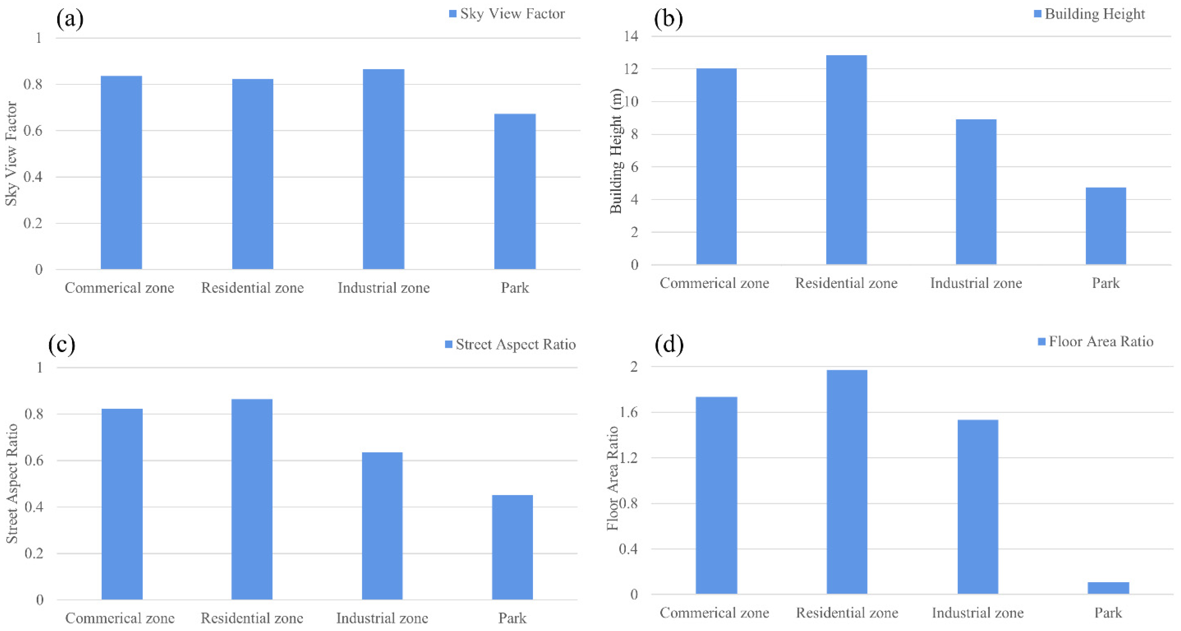
| 3D USP | Sky view factor (SVF) | Sky view factor influenced by building. | [40] |
| Building height (BH) | The height of building | [62] | |
| Street aspect ratio (SAR) | Average building high divided street width | [61] | |
| Floor area ratio (FAR) | Total building floor area divided by block area. | [63] | |
| Spatial pattern | Building Nearest Neighbor Index (BNNI) | The NNI value of buildings | [1] |
| Tree Nearest Neighbor Index (TNNI) | The NNI value of trees | ||
| Grass Nearest Neighbor Index (GNNI) | The NNI value of grasses | ||
| Soil Nearest Neighbor Index (SNNI) | The NNI value of soil lands | [60] | |
| Impervious ground Nearest Neighbor Index (INNI) | The NNI value of impervious grounds | ||
| Water Nearest Neighbor Index (WNNI) | The NNI value of water bodies |
| Experiment | 2D USP | 3D USP | Spatial Pattern Feature |
|---|---|---|---|
| Exp. a | √ | ||
| Exp. b | √ | ||
| Exp. c | √ | ||
| Exp. d | √ | √ | |
| Exp. e | √ | √ | |
| Exp. f | √ | √ | |
| Exp. g | √ | √ | √ |
| Category | RF (%) | KNN (%) | LDA (%) | |||
|---|---|---|---|---|---|---|
| PA | UA | PA | UA | PA | UA | |
| Building | 85.4 | 88.6 | 75.1 | 74.3 | 74.8 | 67.8 |
| Tree | 82.1 | 88.6 | 74.9 | 78.0 | 72.7 | 77.1 |
| Grass | 86.6 | 78.5 | 80.2 | 75.4 | 79.6 | 77.7 |
| Soil | 84.4 | 84.0 | 79.5 | 82.0 | 71.9 | 86.1 |
| Impervious ground | 90.3 | 88.1 | 78.5 | 78.7 | 72.9 | 76.2 |
| Water | 92.6 | 96.9 | 86.8 | 96.7 | 75.0 | 92.7 |
| OA | 87.4 | 77.4 | 74.0 | |||
| Category | RF (%) | KNN (%) | LDA (%) | Average Increase Accuracy (%) | |||
|---|---|---|---|---|---|---|---|
| PA (3D) | PA | PA (3D) | PA | PA (3D) | PA | ||
| Building | 85.4 | 80.6 | 75.1 | 73.5 | 74.8 | 71.4 | 3.3 |
| Tree | 82.1 | 75.2 | 74.9 | 67.3 | 72.7 | 67.1 | 6.7 |
| Grass | 86.6 | 81.5 | 80.2 | 77.8 | 79.6 | 76.3 | 3.6 |
| Soil | 84.4 | 81.7 | 79.5 | 77.7 | 71.9 | 68.3 | 2.7 |
| Impervious ground | 90.3 | 89.5 | 78.5 | 76.8 | 72.9 | 69.7 | 1.9 |
| Water | 92.6 | 91.2 | 86.8 | 83.8 | 75.0 | 73.5 | 2.0 |
| OA | 87.4 | 84.3 | 77.4 | 75.1 | 74.0 | 70.5 | 3.0 |
| Category | RF (%) | KNN (%) | LDA (%) | |||
|---|---|---|---|---|---|---|
| PA | UA | PA | UA | PA | UA | |
| Commercial zone | 89.7 | 78.8 | 72.4 | 61.8 | 75.9 | 73.3 |
| Residential zone | 94.6 | 96.6 | 79.3 | 84.9 | 89.1 | 89.1 |
| Industrial zone | 89.8 | 93.6 | 73.5 | 70.6 | 85.7 | 84.0 |
| Park zone | 87.5 | 88.2 | 68.8 | 73.3 | 75.0 | 85.7 |
| OA | 91.9 | 75.8 | 84.9 | |||
| Method | Data Source | Study Area | OA Value |
|---|---|---|---|
| HSC method [11] | VHR images (0.61m) and POIs | Beijing, China | 90.8% |
| Bottom-up and top-down feedback method [1] | VHR images (0.5 m) | Beijing, China | 84.0% |
| Super object-CNN method [13] | High-resolution images (1.19 m) and POIs | Hangzhou, China | 91.1% |
| Integrating Landsat images and POIs method [12] | Rough resolution images (30m) and POIs | Beijing, China | 81.0% |
| Integrating nighttime light and multi-view imagery method [64] | High-resolution images (5.8m), VHR images (0.92), and POIs | Beijing, China and Wuhan, China | 89.6% (Beijing, China) 85.2% (Wuhan, China) |
| Our method | VHR images (0.3m) and LiDAR data | Brooklyn, New York City, USA | 91.9% |
Publisher’s Note: MDPI stays neutral with regard to jurisdictional claims in published maps and institutional affiliations. |
© 2021 by the authors. Licensee MDPI, Basel, Switzerland. This article is an open access article distributed under the terms and conditions of the Creative Commons Attribution (CC BY) license (https://creativecommons.org/licenses/by/4.0/).
Share and Cite
Sanlang, S.; Cao, S.; Du, M.; Mo, Y.; Chen, Q.; He, W. Integrating Aerial LiDAR and Very-High-Resolution Images for Urban Functional Zone Mapping. Remote Sens. 2021, 13, 2573. https://doi.org/10.3390/rs13132573
Sanlang S, Cao S, Du M, Mo Y, Chen Q, He W. Integrating Aerial LiDAR and Very-High-Resolution Images for Urban Functional Zone Mapping. Remote Sensing. 2021; 13(13):2573. https://doi.org/10.3390/rs13132573
Chicago/Turabian StyleSanlang, Siji, Shisong Cao, Mingyi Du, You Mo, Qiang Chen, and Wen He. 2021. "Integrating Aerial LiDAR and Very-High-Resolution Images for Urban Functional Zone Mapping" Remote Sensing 13, no. 13: 2573. https://doi.org/10.3390/rs13132573
APA StyleSanlang, S., Cao, S., Du, M., Mo, Y., Chen, Q., & He, W. (2021). Integrating Aerial LiDAR and Very-High-Resolution Images for Urban Functional Zone Mapping. Remote Sensing, 13(13), 2573. https://doi.org/10.3390/rs13132573