Article

Modeling of Environmental Impacts on Aerial Hyperspectral Images for Corn Plant Phenotyping

1
Department of Agricultural and Biological Engineering, Purdue University, West Lafayette, IN 47907, USA
2
Health and Crop Sciences Research Laboratory, Sumitomo Chemical Co., Ltd., Takarazuka 665-8555, Hyogo, Japan
3
Department of Agronomy, Purdue University, West Lafayette, IN 47907, USA
*
Author to whom correspondence should be addressed.
Remote Sens. 2021, 13(13), 2520; https://doi.org/10.3390/rs13132520
Submission received: 29 May 2021 / Revised: 21 June 2021 / Accepted: 23 June 2021 / Published: 28 June 2021
(This article belongs to the Special Issue UAVs in Sustainable Agriculture)

Abstract

:
Aerial imaging technologies have been widely applied in agricultural plant remote sensing. However, an as yet unexplored challenge with field imaging is that the environmental conditions, such as sun angle, cloud coverage, temperature, and so on, can significantly alter plant appearance and thus affect the imaging sensor’s accuracy toward extracting plant feature measurements. These image alterations result from the complicated interaction between the real-time environments and plants. Analysis of these impacts requires continuous monitoring of the changes through various environmental conditions, which has been difficult with current aerial remote sensing systems. This paper aimed to propose a modeling method to comprehensively understand and model the environmental influences on hyperspectral imaging data. In 2019, a fixed hyperspectral imaging gantry was constructed in Purdue University’s research farm, and over 8000 repetitive images of the same corn field were taken with a 2.5 min interval for 31 days. Time-tagged local environment data, including solar zenith angle, solar irradiation, temperature, wind speed, and so on, were also recorded during the imaging time. The images were processed for phenotyping data, and the time series decomposition method was applied to extract the phenotyping data variation caused by the changing environments. An artificial neural network (ANN) was then built to model the relationship between the phenotyping data variation and environmental changes. The ANN model was able to accurately predict the environmental effects in remote sensing results, and thus could be used to effectively eliminate the environment-induced variation in the phenotyping features. The test of the normalized difference vegetation index (NDVI) calculated from the hyperspectral images showed that variance in NDVI was reduced by 79%. A similar performance was confirmed with the relative water content (RWC) predictions. Therefore, this modeling method shows great potential for application in aerial remote sensing applications in agriculture, to significantly improve the imaging quality by effectively eliminating the effects from the changing environmental conditions.

1. Introduction

Recent years have seen the rapid growth of remote sensing applications in the field of agriculture [1,2,3]. The advent and advances of low-weight and low-cost imaging platforms, and smart imaging devices resulted in the improved capability of the agricultural data collection. With various sensors such as red-green-blue (RGB), hyperspectral, and thermal cameras carried by these platforms, plant phenotypic properties are captured in images that largely facilitate the process of crop analyses, such as accessing plant biomass, nutrient level, diseases stresses, etc. [1,4,5,6,7,8,9,10]. However, the changing environmental conditions have been reported to significantly impact the imaging results [11]. The intensity of remotely sensed images changes greatly based on when and where the image was captured [12,13,14]. One source of the variation arises from the complicated interactions between the camera’s sensitivity, camera’s view angle, plant canopy geometry, solar zenith angle, solar azimuth angle, and shadows [15,16,17,18]. Another source of variation results from plants’ endogenous stress responses to the environmental conditions, with complicated interactions between their genetic backgrounds, external environments, and treatments [15,19]. All of these, collectively regarded as the environment-induced variation in phenotyping features, affect plants’ final reflectance characteristics.
To reduce the impacts from environment variation, a relatively simple method involves standardizing or fixing the sampling time of the day and restricting imaging to clear conditions without cloud coverage [3,20,21]. Bellvert and Girona [22] suggested that the field phenotypic data should be collected around noon under clear weather conditions. Similarly, unmanned aerial vehicles (UAV) imaging is preferably performed at midday to ensure consistent data collection and analysis [22]. These restrictions could reduce the environmental impacts on the data, but they also significantly inhibit the imaging window and flexibilities. Practically speaking, performing the imaging at a fixed time is difficult, as many procedures, such as equipment setup, need to be completed before imaging and the field environment is naturally uncontrollable and unpredictable. These challenges often result in the collection of remote sensing data at different times of the day under varying environmental conditions. Therefore, the correction of the impact of different imaging time and varying environmental conditions to improve the quality of agricultural remote sensing is critically important to study.
Most aerial remote sensing systems require imaging white reference panels beside the target plants so that the sensing data are calibrated against reference values to remove the illumination variation between images [23]. White reference calibration is effective in compensating different lighting conditions, but these reference images do not precisely reflect the bidirectional reflectance (BRDF) on the leaf surface. Variations from the changes in leaf angles and the plant’s endogenous responses remain. An existing calibration method, the combined PROSPECT leaf optical properties model and SAIL canopy bidirectional reflectance model (PROSAIL) [24], enables the prediction of the plant canopy spectral reflectance changes caused by the changing environmental conditions [17,24]. However, the model usually does not meet the accuracy requirement in plant phenotyping remote sensing [25]. Furthermore, the PROSAIL prediction theoretically requires three input variables, including leaf structure parameter, photosynthetic pigment concertation, and water content, which are difficult and costly to measure in remote sensing practices [26].
Another potential solution arises from the use of different regression methods to predict and compensate for the environmental effects. For example, a correction model with the polynomial regression method was developed to predict the crop reflectance as a function of solar zenith angle, time of day, and instantaneous clearness index (ICI). The capability of the model in reducing the diurnal variation with green normalized difference vegetation index (GNDVI) and some individual bands [27] was tested. However, that model only calibrates the imaging time and ambient lighting factors, while many more environmental condition changes, such as temperature and wind speed, also impact the imaging result. Moreover, the plant data was collected on a small portion of the leaf by a handheld radiometer with four bands, which may not properly simulate airborne remote sensing platforms carrying hyperspectral or multispectral cameras. The simple polynomial regression model could successfully describe the changes in data over three consecutive days. However, it may fail to represent the general pattern on other days when the plants are at different stages of their growth cycle. Therefore, a comprehensive environmental impact analysis for general aerial remote sensing images is still critically needed. This analysis requires the continuous collection of crop images at various plant stages through different environmental conditions, a task that has proven challenging with existing airborne remote sensing systems.
On the modeling method side, the artificial neural network (ANN) models, as opposed to conventional regression models, has received considerable attention because of its ability to learn the features directly from the raw data without prior knowledge and human effort in feature design [28]. Due to their better data utilization capacity, ANN models have outperformed conventional methods for solving regression problems in many ways [29]. For example, researchers have achieved high accuracies and efficiencies on modeling multivariable and time-series datasets [30,31,32]. Given the previous successful applications, an ANN model can prove a reliable and efficient alternative for modeling the environment-induced effects in remote sensing data.
This article introduced the research work of correcting the aerial remote sensing results by modeling and analyzing the effects from the changing field environmental conditions, such as sun radiation, solar zenith angle, humidity, temperature, and wind speed. There are three major objectives in the work of this article:
  • Collect time-series hyperspectral images of two varieties of corn plants with three nitrogen treatments from V4 to R1 every 2.5 min throughout the whole growing season, along with synchronized environmental condition data.
  • Build a prediction model for the environment-induced variation in each of the measured phenotyping features (e.g., NDVI and RWC) with time-series decomposition and ANN method.
  • Evaluate the performance of the trained ANN models and their effects in removing the environmental noise by comparing the variances in the phenotyping features (e.g., NDVI and RWC) before and after the model correction.

2. Materials and Methods

2.1. Experiment Design and Data Collection

To analyze the environmentally induced variation in phenotyping data, hyperspectral images of the crops and environmental data were collected from a corn field in the Purdue University Agronomy Center for Research and Education (ACRE). Two genotypes (B73 × Mo17 and P1105AM) of corn (Zea mays L.) were grown in the summer of 2019. Each genotype was treated with three different nitrogen (N) solutions: high N with 56 kg/ha (32 mL, 28-0-0 in 1L water), medium N with 28 kg/ha (16 mL, 28-0-0 in 1L water), and low N with 0 kg/ha (water). In total, six experimental plots existed, with one of two corn genotypes treated with one of three nitrogen levels; each plot had around 25 plant replicates. The abbreviation for each experimental plot is listed in Table 1.
Hyperspectral images of corn plants were continuously acquired using the Purdue field VNIR hyperspectral imaging gantry system [33]. To capture the instant environmental effects on the images, imaging frequency was set at 2.5 min. Starting from the vegetative growth stage, V4, the continuous imaging occurred for 31 consecutive days until the plants reached the reproductive stage, R1 (Figure 1). Every day, imaging started at 8:00 am and ended at 7:30 pm. In total, we collected 8631 hyperspectral images of the same crop field (Table 2) for this study. After data collection, the hyperspectral images were further processed to measure the plant phenotyping features of interest, including the reflectance spectrum, NDVI, and predicted RWC for each experimental plot. The reflectance spectrum was obtained from the averaged data of plant tissues using the image segmentation algorithm highlighted in [34]. The NDVI was calculated from the spectrum by following Equation (1) [35,36]. The plant’s RWC was predicted with the pretrained partial least squares regression (PLSR) model [33].
N D V I = R 800 n m R 650 n m R 800 n m + R 650 n m
In addition to the hyperspectral imaging data, a local miniature weather station (Ambient Weather, Chandler, AZ, USA) was installed within the experimental plots to collect real-time time-tagged environmental data. The environmental data included air temperature ( ), solar radiation (W/m2), wind speed (m/s), sun zenith angle (degree), humidity (%), and diurnal time (min) (Table 2).

2.2. Time Series Decomposition for Environment-Induced Variation

The phenotyping data from 31 days were collected to provide enough images under various environmental conditions. However, besides the instant environmental effects, the plant growth change and other day-by-day gradual weather changes also contributed to the variation among the images. These different components of variation need to be clearly separated before we can focus on modeling the instant environmental effects. As most of the field environment factors fluctuate over the course of a single day [37,38], we hypothesized that the higher frequency environment-induced variation could be identified by removing the lower frequency variation as the day-to-day trend. Thus, a time series decomposition method was applied, decomposing the original time-series phenotyping signal into two major parts: day-to-day trend ( T t ) and daily instant changes ( D t ) (Equation (2)). More specifically, T t is calculated with the locally estimated scatterplot smoothing (LOESS) method [39]. By fitting a non-parametric regression curve on the scattered plot of the data, the day-to-day changing trend can be extracted from the raw signal [40]. This trend mostly reflects the changes in the plant growth stage and general weather conditions over the 31 days of imaging. The daily instant changes ( D t ) were calculated by subtracting the day-to-day trend ( T t ) from the raw signal. D t contains the higher frequency variation components mostly caused by the plant’s circadian behavior and environmental condition changes such as sun angle, solar radiation, and temperature changes during the day. In this study, D t was used as the output of the proposed model.
R a w   t i m e   s e r i e s   m e a s u r e m e n t s = T t + D t

2.3. Environmental Data Transformation and Selection

To generate more discriminatory power in higher-dimensional feature spaces besides the original environmental variables (temperature, solar zenith angle, wind speed, etc.) for improved model accuracy, a feature transformation was performed by taking the square and square root of the measurements of the original environment factors [41]. These new non-linear variables have proven more effective in modeling environment variation [27]. Finally, the transformed variables were combined with the original variables for further processing.
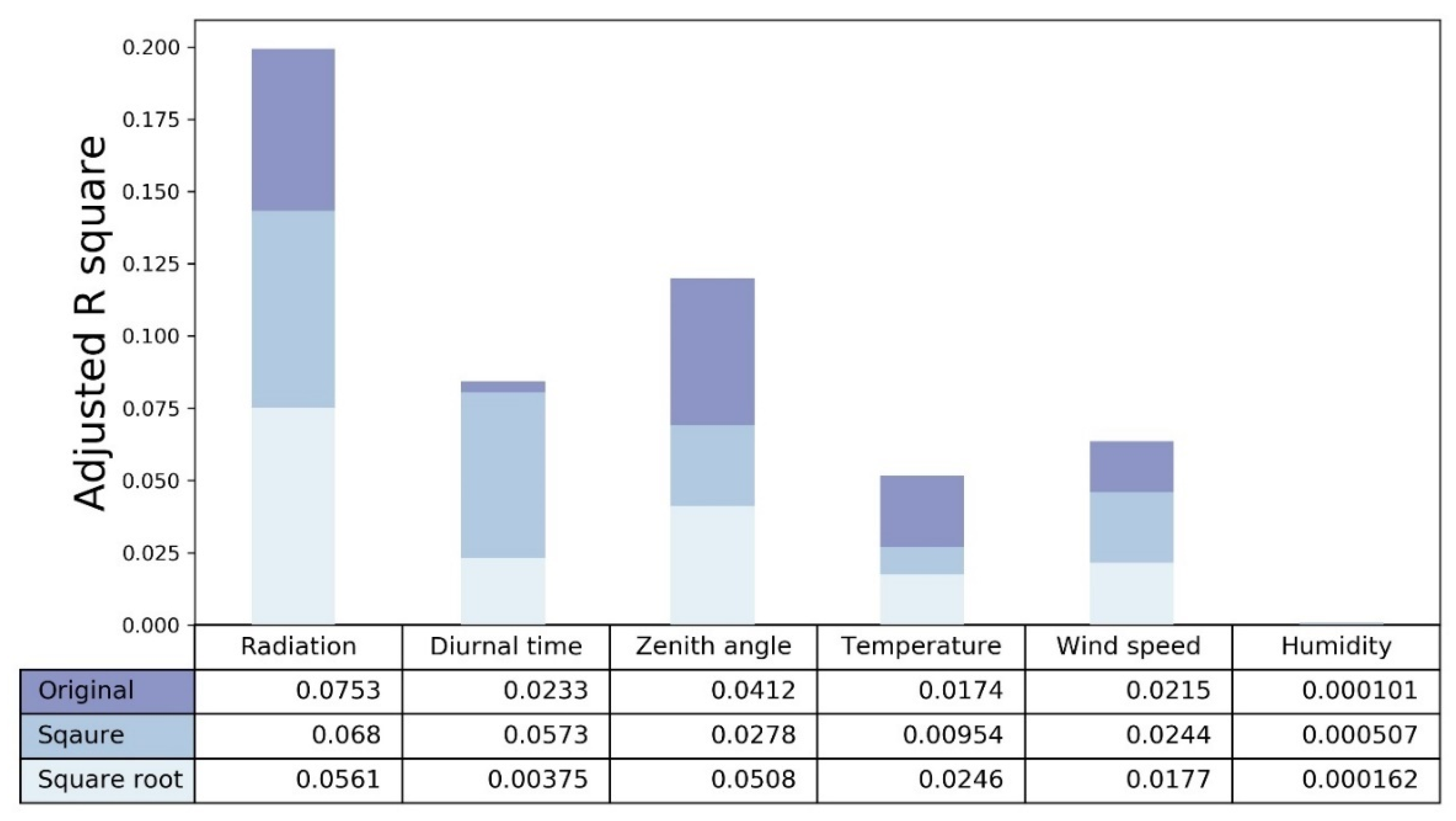
After transformation, the features were selected to remove the irrelevant input of some environmental variables to reduce overfitting. This also lowered the difficulty of future applications, with fewer measurements required. A single-factor correlation analysis was performed. Each of the original or transformed environment variables was fitted with the calculated environment-induced variation in phenotyping data (daily instant changes D t in Equation (2)) in a linear regression model. The adjusted R2, which indicates the relevance of each feature to the estimated environmental variation, was calculated. A higher adjusted R2 meant a variable was more relevant [42]. By comparing the adjusted R2 of each variable, we determined the final list of input environmental variables for the model.

2.4. Data Quality Check

Training data quality is critically important for a supervised machine learning model. The data quality was checked before training the model, and the outlier data was removed [43]. For each phenotyping feature (NDVI and predicted RWC, etc.), the daily measurements between the upper inner fence (Q3+1.5IQR) and lower inner fence (Q1-1.5IQR) were kept [43]. IQR is the interquartile range, which equals the difference between the 75th (Q3) and 25th (Q1) percentiles. Meanwhile, image data before 10:00 am and after 5:30 pm was also removed, as it demonstrated extreme variance and noise [33]. Using the NDVI as an example, we employed the training data sizes shown in Table 3 to train the ANN model.

2.5. Artificial Neural Network (ANN) Model

2.5.1. Architecture

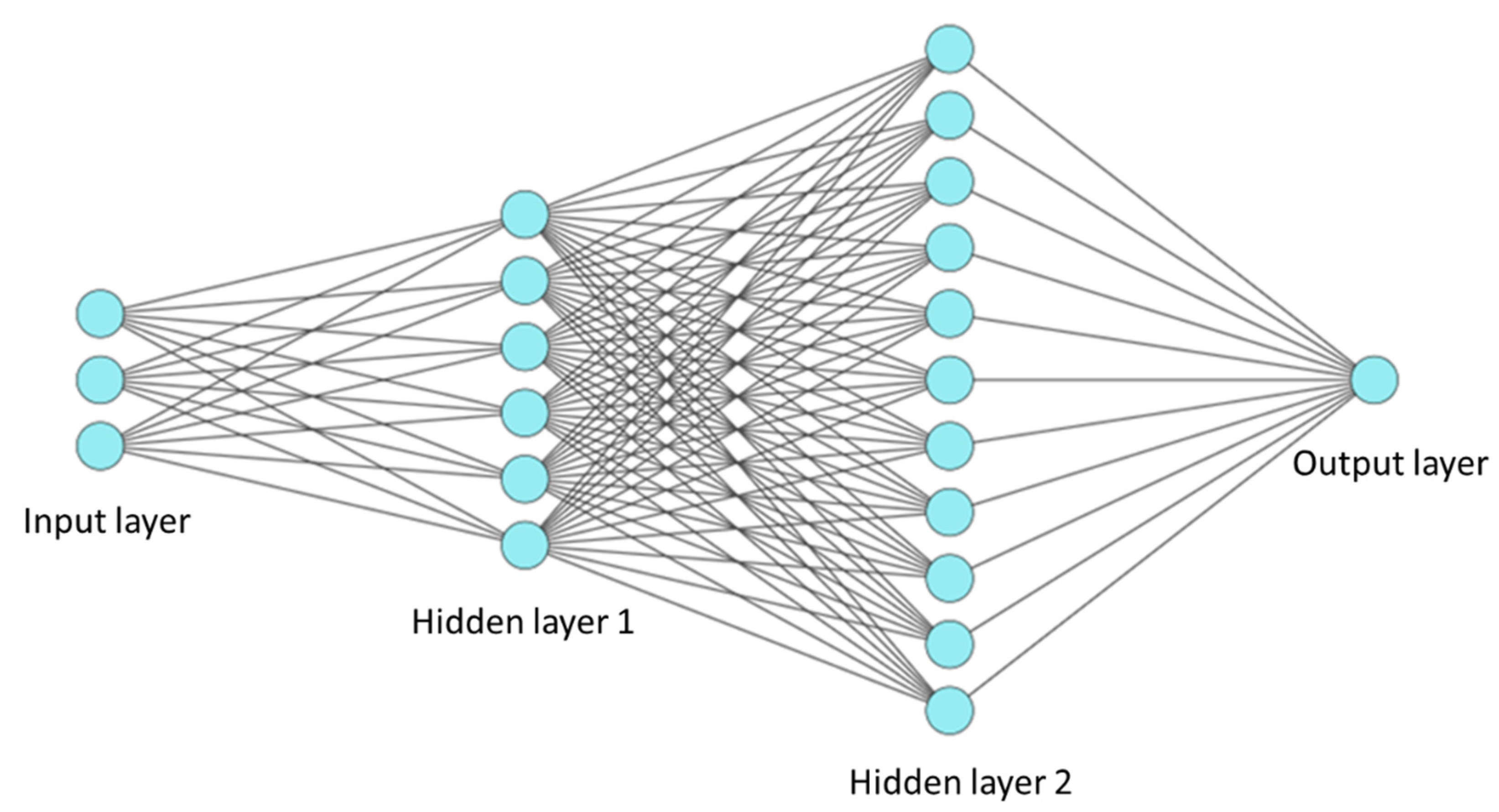
The architecture of the proposed model is based on a feed-forward multi-layer perceptron (MLP) network, a class of ANN models (Figure 2). Due to their adjustable architecture, MLP models are particularly flexible. This flexibility increases the suitability of MLP for regression prediction problems where a real-valued quantity is predicted, given a set of inputs such as time-series data [44]. In this study, after some speed-accuracy tradeoff pretests on model performance, the proposed ANN architecture was configured with a four-layer model containing an input layer, two hidden layers, and an output layer. After each hidden layer, the Leaky ReLU activation was performed to add non-linear properties to the function [45]. The selected environmental variables served as input for the model, whereas the D t environment-induced variation of selected phenotyping features was the output. To accelerate learning and lead to a faster convergence, both input and output data were normalized for modeling purposes [46], while the final prediction results were denormalized back to the original scale of the phenotyping feature.

2.5.2. Training and Optimization

To train the network with minimum overfitting, the training process followed a five-fold cross-validation scenario. We randomly divided the whole dataset into five roughly equal subsets. In the first iteration, the first subset was used to test the model and the rest aided in training the model. This process was repeated until each subset has been used as the testing set. During training, the loss function was Mean Square Error (MSE). The network was initialized with the Kaiming weights [47]. All the ANN models were trained using the Adam optimizer [48].
The accuracy of the model was optimized by adjusting the learning rate, batch size, and the number of epochs. The learning rate controls the rate or speed at which the model learns [49]. The batch size establishes the accuracy of the error gradient estimate when training neural networks [50,51]. The number of epochs impacts the ability of the model to be generalized by determining how many times the model trains on the same data. Finally, by comparing the accuracy (R2 and RMSE) of models with different combinations of the learning rate, batch size, and number of epochs, the model parameters with a batch size of 600 for 120 epochs with learning rate at 1e-3 were chosen for this study.

2.6. Performance Evaluation

2.6.1. Evaluation Metrics

The performance of all the developed models was evaluated and compared with the coefficient of determination (R2) and root mean square error (RMSE) between the prediction results and the original measurements. Meanwhile, we also compared the daily variances of the selected phenotyping features (e.g., NDVI) before and after the model correction. A two-sample t-test was performed to check if daily variance in features fell significantly.

2.6.2. Multi-Model Comparison Analysis across Genotypes and Nitrogen Treatments

The impacts of nitrogen treatments and genotypes on the ANN modeling were also investigated to determine whether a separate ANN model was needed for each case or if one general ANN model could fit the different treatments and genotypes. The ANN model of each experimental plot was trained separately (Table 3) and was tested on the other treatments and genotypes. We also built a general ANN model containing the entire sample data to provide a unified and general “all-in-one” correction approach. With the group-to-group cross-validation on each of the datasets, the R2 and RMSE of each model’s performance in the other datasets were examined to evaluate the generalization of models across genotypes and nitrogen treatments. For example, if the ANN model (ALL) resulted in similar outcomes as the individual plot models (G1H, G1M, G1L, G2H, G2M, G2L) for each plant plot, this unified model would be adopted. Otherwise, different models should be adopted separately for each different case. The aim was to find the most appropriate correction solution as the best balance between ease of use and accuracy.

2.6.3. Phenotyping Features for Testing the Model and Workflow

To demonstrate the detailed modeling procedures and performance evaluation, NDVI was chosen as the first example as it represents one of the most common plant features in remote sensing [52]. We also then tested the same ANN architecture and workflow on the RWC to validate the generalization of the proposed method.

2.7. Software and Computation

All the imaging processing work was implemented with Matlab R2018a software [53]. The modeling work was performed in the Python version 3.7.2 software environment [54]. The ANN model was implemented in PyTorch 0.4.1 [55]. The time-series data was analyzed and manipulated using Pandas [56] and Numpy [57]. The figures were drawn with Seaborn [58] and Matplotlib [59]. The Matlab and Python computations were all executed on a ThinkPad workstation P300 (Lenovo PC international, Morrisville, Morrisville, NC, USA) equipped with 16-gigabytes (GB) of random-access memory (RAM), a 3.70 GHz Intel® Xeon™ E1270 processor, and Nvidia GTX 1070 GPU.

3. Results

3.1. Time Series Decomposition Result

The time-series data of raw NDVI was successfully decomposed into the day-to-day trend ( T t ) and daily instant changes ( D t ) (Figure 3). The raw NDVI plot (row 1 in Figure 3) captured the variation in NDVI over the daytime period, with gaps indicating the time between 5:30 in the afternoon until 10:00 next day without imaging data. The raw NDVI plot showed a clear and repetitive V-shaped pattern for each day, which was caused by environment variation during imaging. The day-to-day trend, T t (row 2 in Figure 3), represented the changes of plant growth stage and plant health conditions. As plants mature, the NDVI was expected to increase until the reproductive stage. Meanwhile, the two big dips along the T t curve precisely captured the impacts from two severe temperature drops in the West Lafayette area. This kind of long-term environmental impact was not included in the proposed analysis.
On the other hand, the daily instant changes ( D t ) (row 3 in Figure 3) showed clear periodical changes with V shapes. Due to the extreme weather conditions, parts of the data were missing on DAP 36, 37, 58, 59, and 60. Overall, D t remained substantially consistent through 31 days, while amplitude and minor skewness differences existed among the D t from different imaging days. For example, the D t of DAP 42 demonstrates a smaller amplitude than that of DAP 56. These differences were caused by different environmental conditions, which would be addressed by the environmental correction model in this study.

3.2. Environmental Feature Selection and Range

The results of the single-factor correlation analysis for NDVI are shown in Figure 4. The environmental variables were all correlated with the environment-induced variation in NDVI, except for humidity and its derivatives. The adjusted R2 values for humidity were almost 0, indicating no correlation found between humidity and NDVI changes. This confirmed the findings from the previous literature that while plant-sensing data were strongly impacted by environment factors such as air temperature, solar radiation, sun zenith angle, and diurnal time [17,27,60], humidity was rarely reported to demonstrate a similar impact. Thus, we removed humidity and its derivatives in the model. Finally, the input feature for each modeling sample was a 1-by-15 vector consisting of air temperature, solar radiation, wind speed, solar zenith angle, diurnal time, and their square or square root values. Besides, the range in environmental conditions experienced by the modeling data was shown in Table 4. These ranges illustrate the appropriate environmental condition to apply the model.

3.3. Performance of the ANN Models

3.3.1. Overall Performance

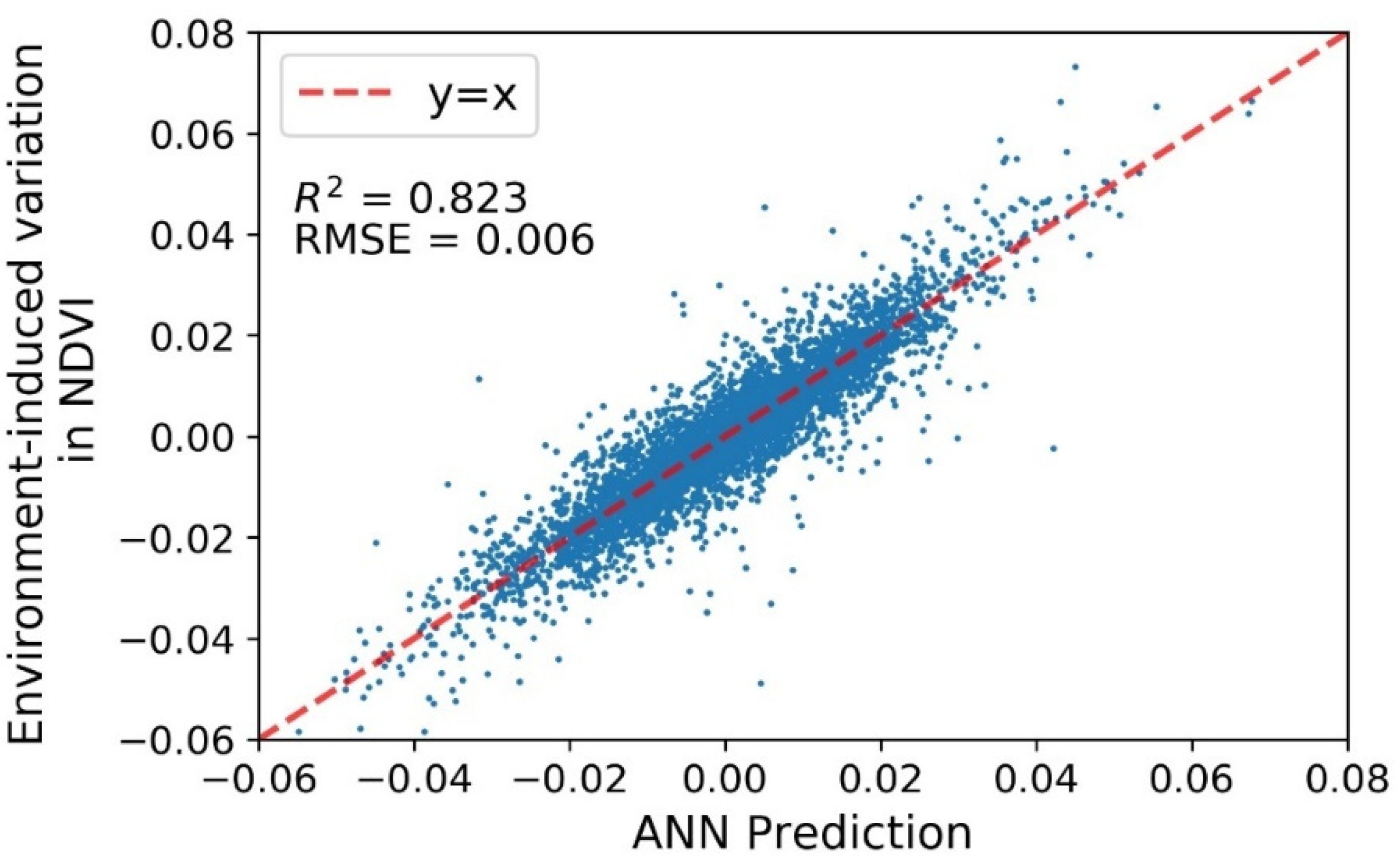
The R2 and RMSE measure the precision of the predicted environment-induced variation in NDVI. The environment-induced variation predicted by the ANN model for the sample dataset (G1H) showed a fairly accurate linear relationship with the coefficient of determination (R2) equal to 0.823 (Figure 5). The RMSE also demonstrated a relatively low value of 0.00611. The prediction result was five-fold cross-validated.
The predicted environmentally induced variation was further used to correct the noise caused by environmental effects in the raw NDVI signal. Figure 6 shows the NDVI corrected by subtracting the predicted variation (Figure 5) from the raw NDVI. In Figure 6b, each box represents the NDVI changes within a day. The trained ANN model largely eliminated the daily variance in the NDVI, so the boxes of the corrected NDVI (Figure 6b) were much more condensed compared with the original NDVI (Figure 6a). To facilitate the comparison, we compared the variances of NDVI before and after model correction with a two-sample t-test (Figure 7 and Table 5). The result confirmed that the daily variances in NDVI were significantly reduced (p-value < 0.01) by 79% on average, thereby confirming the ability of the proposed ANN model to effectively eliminate the environmentally induced effects on the raw signal.

3.3.2. Multi-Model Comparison Analysis across Genotypes and Nitrogen Treatments

The ANN models built for each dataset were tested on the other datasets to evaluate the drifts between different genotypes and nutrient treatments. For datasets from a different genotype or treatment, the ANN model demonstrated a weaker prediction performance compared to the results on dataset it had been trained with (Figure 8). Notably, the predictions were least accurate when the ANN models trained with nitrogen-stressed plots (G1M, G2M, G1L, and G2L) were applied to the high-nitrogen groups (G1H and G2H), as shown within the red boxes in the Figure 8. The results of the multi-model comparison indicate that the nitrogen stress levels on plants should be considered when modeling the environment-induced variation in phenotyping features. Compared to the nitrogen treatments, the genotype difference demonstrated a minor impact. The R2 between plots with the same nitrogen treatment but different genotypes were between 0.59–0.79 with RMSE between 0.009–0.013. The general ANN model (ALL) trained with the entire sample data performed well across the different genotypes and treatments with substantially high R2 (0.617–0.843) and low RMSE values (0.008–0.0010). This allowed us to apply the same one ANN model (ALL) for diverse corn stages (already included in the modeling), genotypes, and treatments (validated in Figure 8).

3.4. Modeling of Environmentally Induced Variation in Predicted RWC

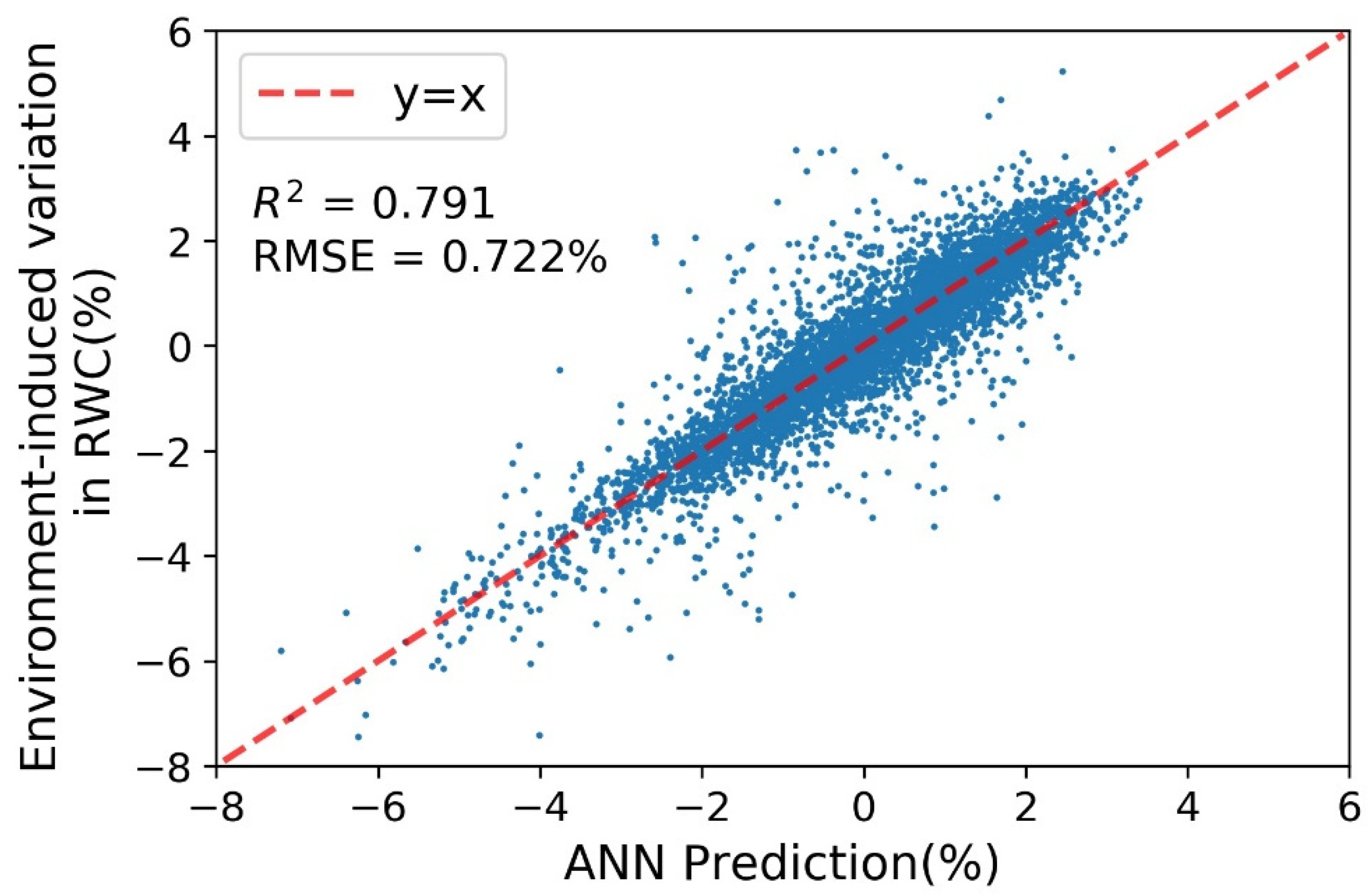
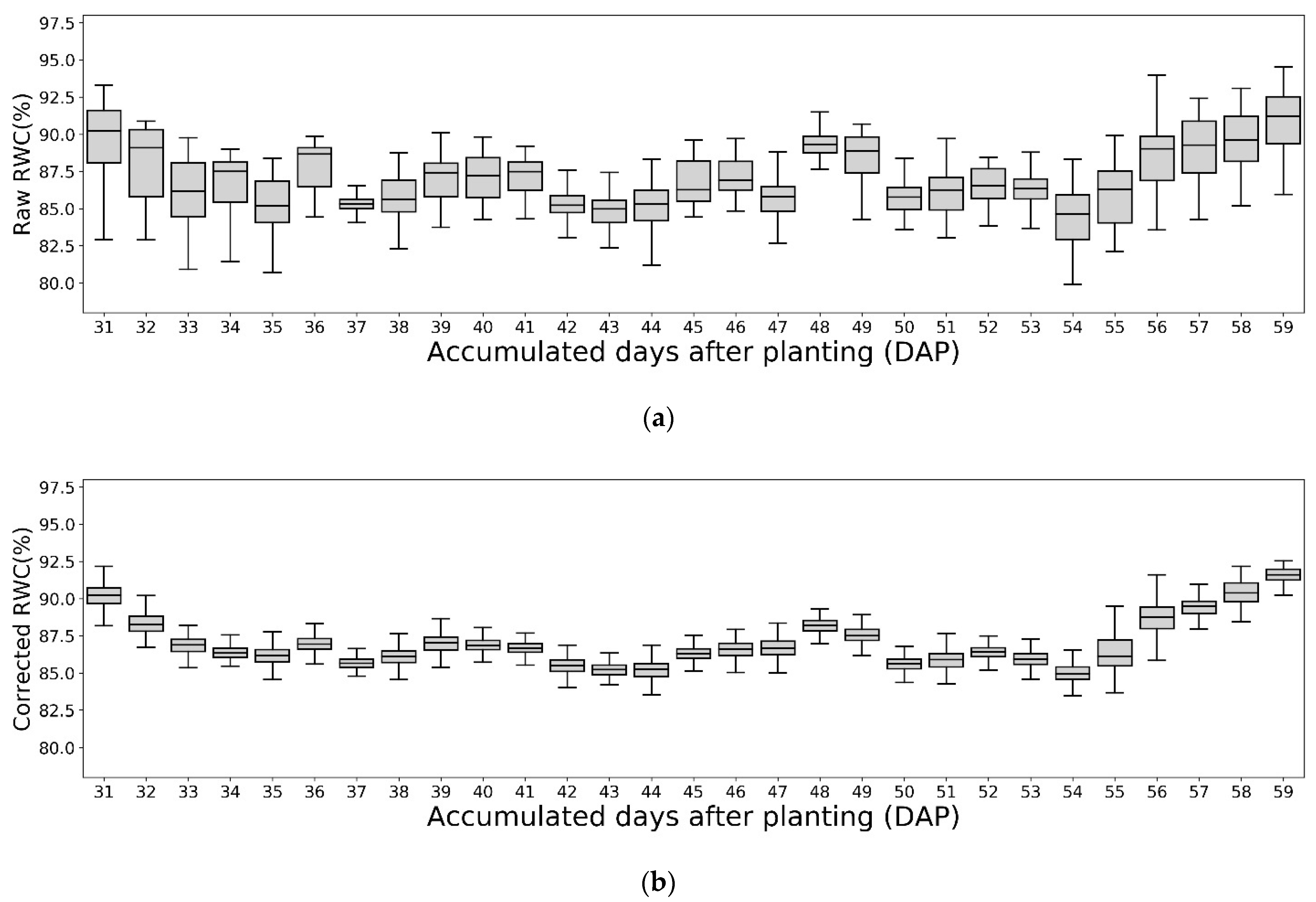
Besides NDVI, the environmentally induced variation in the predicted RWC was also modeled and predicted. In Figure 9, the predicted and the measured variation were strongly correlated, with a R2 of 0.791 and RMSE of 0.722%. With this model, the variance of the corrected RWC was significantly reduced (p-value < 0.01) by 72% on average compared to the raw predicted RWC data (Figure 10). The successful application of the same proposed ANN architecture and decomposition method on the predicted RWC and NDVI indicated that this method has the potential to be generally applied on other phenotyping features that can be further explored. Moreover, the corrected predicted RWC plot (Figure 10b) demonstrates a more obvious day-to-day trend than the raw predicted RWC (Figure 10a). Therefore, with the environmental effects removed, plant remote-sensing researchers can more accurately track the plant growth signals.

4. Discussion

Environmental change impacts in crop aerial remote sensing images were quantitatively investigated with the proposed ANN modeling approach. Over 8000 hyperspectral images of two varieties of corn with three nitrogen treatments were taken by the field imaging gantry at Purdue University over the 2019 growing season. The imaging covered the plant stages from V4 to R1. Crop phenotyping features such as NDVI, RWC, and two individual spectral bands (Red and NIR) were calculated from the imaging data. The proposed ANN model was trained with synchronized hyperspectral imaging data and environmental data (including sun radiation, solar zenith angle, diurnal time, temperature, and wind speed) to understand the correlation of the variations between the two datasets. A time-series decomposition method was applied to extract the phenotyping data variation caused by the changing environments. By learning the relationship between the phenotyping data variation and environmental changes, the developed ANN model was able to precisely predict the environmental effects on remote sensing results (i.e., 82.2% for NDVI), and thus could be used to effectively eliminate the environment-induced variation in the phenotyping features. The two-sample t-tests on the NDVI and predicted RWC of corn plants showed that the daily variances in NDVI and predicted RWC were significantly reduced by 79% and 72%, respectively. Thus, the ANN method can be used by remote sensing professionals to adjust or correct raw imaging data for changing environments to improve plant characterization.
The proposed ANN-based method showed a promising performance in modeling the environment-induced variations in different plant phenotyping features. However, the data used in the model was drawn from one single field test whose imaging data was collected from Purdue’s field gantry system, which might induce systematic bias in the model. External validation data from the other remote sensing platforms, such as UAVs, are needed. In the next growing season, the proposed method will be validated with images from a field UAV system as well as RGBN camera-based imaging sensor (Ncam) [61]. Furthermore, this modeling method was developed based on corn images, which might limit the scope of application. It is necessary to conduct more tests on more diverse plant species (e.g., soybean, wheat, and rice). This will help further validate the developed models, as well as improve the robustness of the prospective models.
In the future, we will also continue exploring training models for all the single spectral bands to adjust/correct the whole spectrum data considering environmental variations. Remote sensing users could benefit from the spectrum calibration model to correct the prediction results from any plant feature prediction models.

5. Conclusions

In this paper, a new modeling method was successfully proposed to precisely predict the environmental effects on the hyperspectral imaging results (such as NDVI and predicted RWC) in aerial crop remote sensing. Over 8000 hyperspectral images, together with synchronized environment data, were collected over 31 days for field corn plants with different nitrogen treatments and genotypes. Experimental results demonstrated that the proposed ANN method could accurately predict the environment-induced variations in the selected phenotyping features. For example, the trained model for NDVI achieved promising predictive results for the sample dataset with an R2 of 0.822 and an RMSE of 0.00611 compared with the measured variation. The predicted values were used to correct the raw phenotyping data, and the daily variance of NDVI was significantly reduced by 79%. The proposed method also achieved satisfactory results when tested on predicted RWC (daily variance reduced by 72%). The applicability of the proposed method on two different features highlighted its potential to correct the other phenotyping features of interest. Based on these results, this proposed modeling method can help agricultural remote sensing researchers to effectively eliminate the signal drifts caused by the environment variation, which will drastically increase the accuracy of field plant sensing.

Author Contributions

D.M. carried out the data collection, data analysis, and drafted the manuscript; J.J. contributed the research idea, led the designing, fund-raising, and construction of the field imaging facility, designed the experiments, and revised the manuscript; H.M. and M.R.T. guided the experimental design; T.U.R. and L.Z. made substantial contributions to system construction and data collection. All authors have read and agreed to the published version of the manuscript.

Funding

This research was funded by Sumitomo Chemical, grant number 16121941. The APC was funded by Purdue University.

Data Availability Statement

The data presented in this study are available on request from the corresponding author. The data are not publicly available due to confidentiality.

Acknowledgments

The project was sponsored and supported by Sumitomo Chemical and Department of Agricultural and Biological Engineering, Purdue University. The authors would like to thank Meng-Yang Lin (Student, Department of Agronomy, Purdue University) for his assistance in ground truth data collection.

Conflicts of Interest

The authors declare no conflict of interest.

References

  1. Li, L.; Zhang, Q.; Huang, D. A Review of Imaging Techniques for Plant Phenotyping. Sensors 2014, 14, 20078–20111. [Google Scholar] [CrossRef] [PubMed]
  2. Wang, R.; Cherkauer, K.; Bowling, L. Corn Response to Climate Stress Detected with Satellite-Based NDVI Time Series. Remote Sens. 2016, 8, 269. [Google Scholar] [CrossRef] [Green Version]
  3. Gracia-Romero, A.; Kefauver, S.C.; Fernandez-Gallego, J.A.; Vergara-Díaz, O.; Nieto-Taladriz, M.T.; Araus, J.L. UAV and ground image-based phenotyping: A proof of concept with durum wheat. Remote Sens. 2019, 11, 1244. [Google Scholar] [CrossRef] [Green Version]
  4. Zhang, L.; Wang, L.; Wang, J.; Song, Z.; Rehman, T.U.; Bureetes, T.; Ma, D.; Chen, Z.; Neeno, S.; Jin, J. Leaf Scanner: A portable and low-cost multispectral corn leaf scanning device for precise phenotyping. Comput. Electron. Agric. 2019, 167, 105069. [Google Scholar] [CrossRef]
  5. Wang, L.; Jin, J.; Song, Z.; Wang, J.; Zhang, L.; Rehman, T.U.; Ma, D.; Carpenter, N.R.; Tuinstra, M.R. LeafSpec: An accurate and portable hyperspectral corn leaf imager. Comput. Electron. Agric. 2020, 169, 105209. [Google Scholar] [CrossRef]
  6. Ma, D.; Carpenter, N.; Maki, H.; Rehman, T.U.; Tuinstra, M.R.; Jin, J. Greenhouse environment modeling and simulation for microclimate control. Comput. Electron. Agric. 2019, 162, 134–142. [Google Scholar] [CrossRef]
  7. Zhang, L.; Maki, H.; Ma, D.; Sánchez-Gallego, J.A.; Mickelbart, M.V.; Wang, L.; Rehman, T.U.; Jin, J. Optimized angles of the swing hyperspectral imaging system for single corn plant. Comput. Electron. Agric. 2019, 156, 349–359. [Google Scholar] [CrossRef]
  8. Ma, D.; Maki, H.; Neeno, S.; Zhang, L.; Wang, L.; Jin, J. Application of non-linear partial least squares analysis on prediction of biomass of maize plants using hyperspectral images. Biosyst. Eng. 2020, 200, 40–54. [Google Scholar] [CrossRef]
  9. Ma, D.; Wang, L.; Zhang, L.; Song, Z.; Rehman, T.U.; Jin, J. Stress distribution analysis on hyperspectral corn leaf images for improved phenotyping quality. Sensors 2020, 20, 3659. [Google Scholar] [CrossRef]
  10. Rehman, T.U.; Ma, D.; Wang, L.; Zhang, L.; Jin, J. Predictive spectral analysis using an end-to-end deep model from hyperspectral images for high-throughput plant phenotyping. Comput. Electron. Agric. 2020, 177, 105713. [Google Scholar] [CrossRef]
  11. Gamon, J.A.; Kovalchuck, O.; Wong, C.Y.S.; Harris, A.; Garrity, S.R. Monitoring seasonal and diurnal changes in photosynthetic pigments with automated PRI and NDVI sensors. Biogeosciences 2015, 12, 4149–4159. [Google Scholar] [CrossRef] [Green Version]
  12. Padilla, F.M.; de Souza, R.; Peña-Fleitas, M.T.; Grasso, R.; Gallardo, M.; Thompson, R.B. Influence of time of day on measurement with chlorophyll meters and canopy reflectance sensors of different crop N status. Precis. Agric. 2019, 20, 1087–1106. [Google Scholar] [CrossRef] [Green Version]
  13. Beneduzzi, H.M.; Souza, E.G.; Bazzi, C.L.; Schenatto, K. Temporal variability in active reflectance sensor-measured NDVI in soybean and wheat crops. Eng. Agric. 2017, 37, 771–781. [Google Scholar] [CrossRef]
  14. Maji, S.; Chandra, B.; Viswavidyalaya, K. Diurnal Variation in Spectral Properties of Potato under Different Dates of Planting and N-Doses Diurnal Variation in Spectral Properties of Potato under Different Dates of Planting and N-Doses. Environ. Ecol. 2014, 33, 478–483. [Google Scholar]
  15. Ranson, K.J.; Daughtry, C.S.T.; Biehl, L.L.; Bauer, M.E. Sun-view angle effects on reflectance factors of corn canopies. Remote Sens. Environ. 1985, 18, 147–161. [Google Scholar] [CrossRef]
  16. Jackson, R.D.; Pinter, P.J.; Idso, S.B.; Reginato, R.J. Wheat spectral reflectance: Interactions between crop configuration, sun elevation, and azimuth angle. Appl. Opt. 1979, 18, 3730–3732. [Google Scholar] [CrossRef]
  17. Ishihara, M.; Inoue, Y.; Ono, K.; Shimizu, M.; Matsuura, S. The impact of sunlight conditions on the consistency of vegetation indices in croplands-Effective usage of vegetation indices from continuous ground-based spectral measurements. Remote Sens. 2015, 7, 14079–14098. [Google Scholar] [CrossRef] [Green Version]
  18. Danner, M.; Berger, K.; Wocher, M.; Mauser, W.; Hank, T. Fitted PROSAIL parameterization of leaf inclinations, water content and brown pigment content for winter wheat and maize canopies. Remote Sens. 2019, 11, 1150. [Google Scholar] [CrossRef] [Green Version]
  19. An, N.; Welch, S.M.; Markelz, R.J.C.; Baker, R.L.; Palmer, C.M.; Ta, J.; Maloof, J.N.; Weinig, C. Quantifying time-series of leaf morphology using 2D and 3D photogrammetry methods for high-throughput plant phenotyping. Comput. Electron. Agric. 2017, 135, 222–232. [Google Scholar] [CrossRef] [Green Version]
  20. Di Gennaro, S.F.; Rizza, F.; Badeck, F.W.; Berton, A.; Delbono, S.; Gioli, B.; Toscano, P.; Zaldei, A.; Matese, A. UAV-based high-throughput phenotyping to discriminate barley vigour with visible and near-infrared vegetation indices. Int. J. Remote Sens. 2018, 39, 5330–5344. [Google Scholar] [CrossRef]
  21. Barbedo, J.G.A. A Review on the Use of Unmanned Aerial Vehicles and Imaging Sensors for Monitoring and Assessing Plant Stresses. Drones 2019, 3, 40. [Google Scholar] [CrossRef] [Green Version]
  22. Krishna, K.R. Agricultural Drones: A Peaceful Pursuit; Taylor & Francis: Abingdon, UK, 2018. [Google Scholar]
  23. Miura, T.; Huete, A.R. Performance of three reflectance calibration methods for airborne hyperspectral spectrometer data. Sensors 2009, 9, 794–813. [Google Scholar] [CrossRef] [Green Version]
  24. Jacquemoud, S.; Baret, F. PROSPECT: A model of leaf optical properties spectra. Remote Sens. Environ. 1990, 34, 75–91. [Google Scholar] [CrossRef]
  25. Berger, K.; Atzberger, C.; Danner, M.; Wocher, M.; Mauser, W.; Hank, T. Model-based optimization of spectral sampling for the retrieval of crop variables with the PROSAIL model. Remote Sens. 2018, 10, 2063. [Google Scholar] [CrossRef] [Green Version]
  26. Jacquemoud, S.; Verhoef, W.; Baret, F.; Bacour, C.; Zarco-Tejada, P.J.; Asner, G.P.; François, C.; Ustin, S.L. PROSPECT + SAIL models: A review of use for vegetation characterization. Remote Sens. Environ. 2009, 113, S56–S66. [Google Scholar] [CrossRef]
  27. De Souza, E.G.; Scharf, P.C.; Sudduth, K.A. Sun position and cloud effects on reflectance and vegetation indices of corn. Agron. J. 2010, 102, 734–744. [Google Scholar] [CrossRef] [Green Version]
  28. Wang, T.; Rostamza, M.; Song, Z.; Wang, L.; McNickle, G.; Iyer-Pascuzzi, A.S.; Qiu, Z.; Jin, J. SegRoot: A high throughput segmentation method for root image analysis. Comput. Electron. Agric. 2019, 162, 845–854. [Google Scholar] [CrossRef]
  29. Abiodun, O.I.; Jantan, A.; Omolara, A.E.; Dada, K.V.; Mohamed, N.A.E.; Arshad, H. State-of-the-art in artificial neural network applications: A survey. Heliyon 2018, 4, e00938. [Google Scholar] [CrossRef] [Green Version]
  30. Yilmaz, I.; Kaynar, O. Multiple regression, ANN (RBF, MLP) and ANFIS models for prediction of swell potential of clayey soils. Expert Syst. Appl. 2011, 38, 5958–5966. [Google Scholar] [CrossRef]
  31. Mokarram, M.; Bijanzadeh, E. Prediction of biological and grain yield of barley using multiple regression and artificial neural network models. Aust. J. Crop. Sci. 2016, 10, 895–903. [Google Scholar] [CrossRef]
  32. Zhang, Z.; Masjedi, A.; Zhao, J.; Crawford, M.M. Prediction of sorghum biomass based on image based features derived from time series of UAV images. Int. Geosci. Remote Sens. Symp. 2017, 2017, 6154–6157. [Google Scholar] [CrossRef]
  33. Ma, D.; Rehman, T.U.; Zhang, L.; Jin, J. Modeling of diurnal changing patterns in airborne crop remote sensing images. Remote Sens. 2021, 13, 1719. [Google Scholar] [CrossRef]
  34. Ma, D.; Carpenter, N.; Amatya, S.; Maki, H.; Wang, L.; Zhang, L.; Neeno, S.; Tuinstra, M.R.; Jin, J. Removal of greenhouse microclimate heterogeneity with conveyor system for indoor phenotyping. Comput. Electron. Agric. 2019, 166, 104979. [Google Scholar] [CrossRef]
  35. Schafleitner, R.; Gutierrez, R.; Espino, R.; Gaudin, A.; Pérez, J.; Martínez, M.; Domínguez, A.; Tincopa, L.; Alvarado, C.; Numberto, G.; et al. Field screening for variation of drought tolerance in Solanum tuberosum L. by agronomical, physiological and genetic analysis. Potato Res. 2007, 50, 71–85. [Google Scholar] [CrossRef]
  36. Daughtry, C.S.T.; Walthall, C.L.; Kim, M.S.; De Colstoun, E.B.; McMurtrey Iii, J.E. Estimating corn leaf chlorophyll concentration from leaf and canopy reflectance. Remote Sens. Environ. 2000, 74, 229–239. [Google Scholar] [CrossRef]
  37. Weatherley, P.E. Studies in the Water Relations of the Cotton Plant. II. Diurnal and Seasonal Variations in Relative Turgidity and Environmental Factors. New Phytol. 1951, 50, 36–51. [Google Scholar] [CrossRef]
  38. Zhou, X.; Xu, Y.; Zhang, F. Evaluation of effect of diurnal ambient temperature range on solar chimney power plant performance. Int. J. Heat Mass Transf. 2017, 115, 398–405. [Google Scholar] [CrossRef]
  39. Rojo, J.; Rivero, R.; Romero-Morte, J.; Fernández-González, F.; Pérez-Badia, R. Modeling pollen time series using seasonal-trend decomposition procedure based on LOESS smoothing. Int. J. Biometeorol. 2017, 61, 335–348. [Google Scholar] [CrossRef] [PubMed]
  40. Cleveland, R.B.; Cleveland, W.S.; McRae, J.E.; Terpenning, I. STL: A seasonal-trend decomposition. J. Off. Stat. 1990, 6, 3–73. [Google Scholar]
  41. Kusiak, A. Feature transformation methods in data mining. IEEE Trans. Electron. Packag. Manuf. 2001, 24, 214–221. [Google Scholar] [CrossRef]
  42. Helland, I.S. On the interpretation and use of R2 in regression analysis. Biometrics 1987, 43, 61–69. [Google Scholar] [CrossRef]
  43. Schwertman, N.C.; de Silva, R. Identifying outliers with sequential fences. Comput. Stat. Data Anal. 2007, 51, 3800–3810. [Google Scholar] [CrossRef]
  44. Mellit, A.; Pavan, A.M. A 24-h forecast of solar irradiance using artificial neural network: Application for performance prediction of a grid-connected PV plant at Trieste, Italy. Sol. Energy 2010, 84, 807–821. [Google Scholar] [CrossRef]
  45. Sharma, S.; Sharma, S. Activation functions in neural networks. Data Sci. 2017, 6, 310–316. [Google Scholar] [CrossRef]
  46. Zhang, X.; Sugano, Y.; Bulling, A. Revisiting data normalization for appearance-based gaze estimation. Eye Track. Res. Appl. Symp. 2018. [Google Scholar] [CrossRef] [Green Version]
  47. He, K.; Zhang, X.; Ren, S.; Sun, J. Delving deep into rectifiers: Surpassing human-level performance on imagenet classification. In Proceedings of the 2015 IEEE International Conference on Computer Vision (ICCV), Santiago, Chile, 7–13 December 2015; pp. 1026–1034. [Google Scholar]
  48. Le, Q.V.; Ngiam, J.; Coates, A.; Lahiri, A.; Prochnow, B.; Ng, A.Y. On optimization methods for deep learning. In Proceedings of the 28th International Conference on Machine Learning, ICML 2011, Washington, DC, USA, 28 June–2 July 2011. [Google Scholar]
  49. Jacobs, R.A. Increased rates of convergence through learning rate adaptation. Neural Netw. 1988, 1, 295–307. [Google Scholar] [CrossRef]
  50. Gholamrezaei, M.; Ghorbanian, K. Rotated general regression neural network. In Proceedings of the 2007 International Joint Conference on Neural Networks, Orlando, FL, USA, 12–17 August 2007; Volume 2, pp. 1959–1964. [Google Scholar] [CrossRef]
  51. Livingstone, D.J. Artificial Neural Networks: Methods and Applications; Springer: Berlin/Heidelberg, Germany, 2008. [Google Scholar]
  52. Cabrera-Bosquet, L.; Molero, G.; Stellacci, A.; Bort, J.; Nogués, S.; Araus, J. NDVI as a potential tool for predicting biomass, plant nitrogen content and growth in wheat genotypes subjected to different water and nitrogen conditions. Cereal Res. Commun. 2011, 39, 147–159. [Google Scholar] [CrossRef]
  53. The MathWorks Inc. MATLAB Version 9.4.0.813654 (R2018a); The MathWorks Inc.: Natick, MA, USA, 2018. [Google Scholar]
  54. Van Rossum, G.; Drake, F.L. Python 3 Reference Manual; CreateSpace: Scotts Valley, CA, USA, 2009; ISBN 1441412697. [Google Scholar]
  55. Paszke, A.; Gross, S.; Chintala, S.; Chanan, G.; Yang, E.; DeVito, Z.; Lin, Z.; Desmaison, A.; Antiga, L.; Lerer, A. Automatic differentiation in PyTorch. In Proceedings of the NIPS 2017 Workshop Autodiff Submission, Long Beach, CA, USA, 28 October 2017. [Google Scholar]
  56. McKinney, W. Data structures for statistical computing in python. In Proceedings of the 9th Python in Science Conference, Austin, TX, USA, 28 June–3 July 2010; Volume 445, pp. 51–56. [Google Scholar]
  57. Oliphant, T.E. A Guide to NumPy; Trelgol Publishing: USA, 2006; Volume 1, Available online: https://web.mit.edu/dvp/Public/numpybook.pdf (accessed on 29 May 2021).
  58. Waskom, M.; Botvinnik, O.; O’Kane, D.; Hobson, P.; Lukauskas, S.; Gemperline, D.C.; Augspurger, T.; Halchenko, Y.; Cole, J.B.; Warmenhoven, J.; et al. mwaskom/seaborn: v0.8.1 (September 2017). Zenodo 2017. [Google Scholar] [CrossRef]
  59. Hunter, J.D. Matplotlib: A 2D graphics environment. Comput. Sci. Eng. 2007, 9, 90–95. [Google Scholar] [CrossRef]
  60. Jones, H.G.; Serraj, R.; Loveys, B.R.; Xiong, L.; Wheaton, A.; Price, A.H. Thermal infrared imaging of crop canopies for the remote diagnosis and quantification of plant responses to water stress in the field. Funct. Plant Biol. 2009, 36, 978–989. [Google Scholar] [CrossRef] [Green Version]
  61. Wang, L.; Duan, Y.; Zhang, L.; Rehman, T.U.; Ma, D.; Jin, J. Precise Estimation of NDVI with a Simple NIR Sensitive RGB Camera and Machine Learning Methods for Corn Plants. Sensors 2020, 20, 3208. [Google Scholar] [CrossRef]
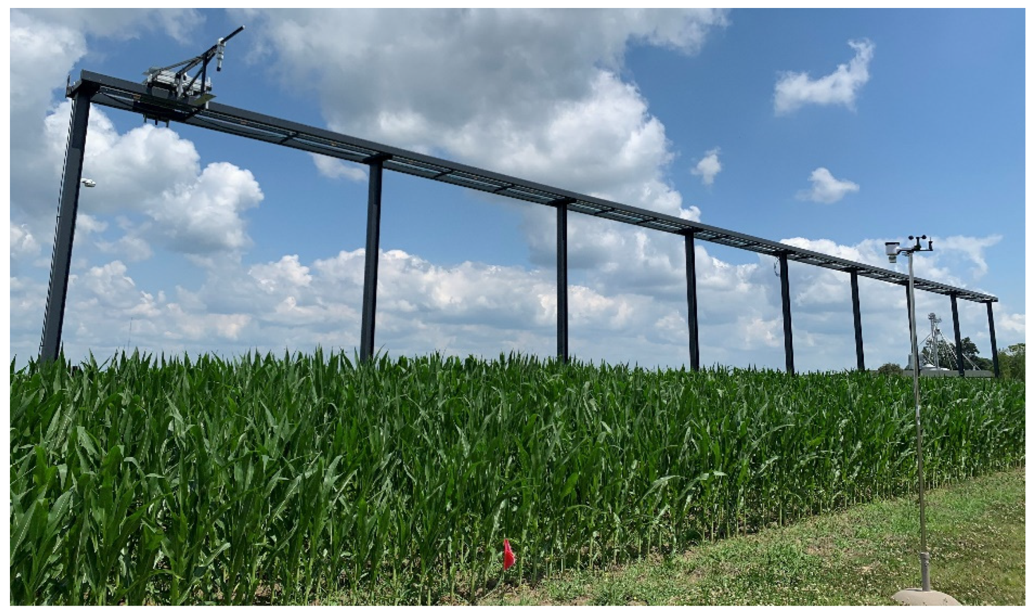
Figure 1. Field VNIR hyperspectral platform at Purdue University. It consists of a VNIR hyperspectral imaging sensor (MSV-101-W, Middleton Spectral Vision, Middleton, WI, USA) and a local weather station (Ambient Weather, Chandler, AZ, USA). The gantry platform is seven meters high and capable of scanning all or part of a 50-by-5 m strip field under a wide range of weather conditions.
Remotesensing 13 02520 g001
Figure 2. The ANN architecture: Input layer (15 neurons); Hidden layer 1 (100 neurons, followed with Leaky ReLU); Hidden layer 2 (1000 neurons, followed with Leaky ReLU); Output layer (1 neuron).
Remotesensing 13 02520 g002
Figure 3. The NDVI of the sample dataset (G1H) from the V4 stage to the R1 stage. The raw NDVI plot was decomposed into the day-to-day trend ( T t ) and the periodic change ( D t ). The red boxes are the days with incomplete data measurements due to the extreme weather conditions, which are DAP 36, 37, 58, 59, and 60.
Remotesensing 13 02520 g003
Figure 4. Single-factor correlation analysis for NDVI. The x-axis is the environment factors and their squared or root squared formats. The y-axis is the adjusted R2 between each x variable and the calculated environment-induced variation in NDVI. Larger adjusted R2 value means the variable is more correlated to the NDVI variation.
Remotesensing 13 02520 g004
Figure 5. The five-fold cross-validated prediction results of environment-induced variation in NDVI for the sample dataset (G1H). The ANN prediction values show a significant correlation with R2 = 0.823 and RMSE = 0.006.
Remotesensing 13 02520 g005
Figure 6. Box plots for the five-fold cross-validated correction result of the sample dataset (G1H). (a) The raw NDVI with huge daily variances across 31 days. (b) The ANN model corrected NDVI with much more condensed boxes.
Remotesensing 13 02520 g006
Figure 7. Two-sample t-test between the variance of daily NDVI for the sample dataset (G1H) before and after ANN model correction.
Remotesensing 13 02520 g007
Figure 8. Accuracy heatmaps of R2 and RMSE of ANN models for NDVI. Red boxes: the region with relatively poor predictive results.
Remotesensing 13 02520 g008
Figure 9. The five-fold cross-validated prediction results of environment-induced variation in predicted RWC for the sample dataset (G1H). The ANN prediction values show a significant performance with R2 = 0.791 and RMSE = 0.722%.
Remotesensing 13 02520 g009
Figure 10. Box plots for the five-fold cross-validated correction result of sample dataset (G1H). (a) The raw predicted RWC showed huge daily variances across 31 days. (b) The ANN model corrected predicted RWC has much more condensed boxes.
Remotesensing 13 02520 g010
Table 1. Abbreviations of plant plots with different nitrogen treatments and genotypes.
Plant GroupsGenotypesN TreatmentsAbbrev
1B73 × Mo17 (Genotype 1)HighG1H
2B73 × Mo17 (Genotype 1)MediumG1M
3B73 × Mo17(Genotype 1)LowG1L
4P1105AM (Genotype 2)HighG2H
5P1105AM (Genotype 2)MediumG2M
6P1105AM (Genotype 2)LowG2L
1–6 combinedAll combinedAll combinedAll
Table 2. Hyperspectral images and environmental data collection.
Data CollectionSampling Days# SamplesVariables
Hyperspectral images318631VNIR Spectra: 376–1044 nm with 1.22 nm interval.
Environmental data318631Air temperature (°C)
Sun radiation (W/m2)
Wind speed (m/s)
Solar zenith angle (degree)
Humidity (%)
Diurnal time (min)
Table 3. Data pool after data quality check.
DatasetsNumber of Samples before the Quality CheckNumber of Samples after the Quality Check
G1H86315070
G1M86315092
G1L86315083
G2H86315108
G2M86315084
G2L86315093
All51,78930,530
Table 4. The ranges in environmental conditions experienced by the modeling data during the experiment.
Environmental VariablesMinMax
Sun radiation (W/m2)85.76954.23
Diurnal time (min)600 (at 10 a.m.)1050 (at 5:30 p.m.)
Solar zenith angle (degree)35.278.26
Air temperature (°C)11.7933.27
Wind speed (m/s)08.3
Humidity (%)26.5297.06
Note: Diurnal time counts from midnight, so the value at midnight is 0 min.
Table 5. The results of the two-sample t-test between the variance of daily NDVI before and after ANN model correction.
GroupsNMeanStDevSE MeanT-Valuep-Value
Raw NDVI310.0002300.0001740.0000315.78<0.01
Corrected NDVI310.00004720.00002480.0000045
Publisher’s Note: MDPI stays neutral with regard to jurisdictional claims in published maps and institutional affiliations.