Abstract
In precision agriculture, efficient fertilization is one of the most important pursued goals. Vegetation spectral profiles and the corresponding spectral parameters are usually employed for vegetation growth status indication, i.e., vegetation classification, bio-chemical content mapping, and efficient fertilization guiding. In view of the fact that the spectrometer works by relying on ambient lighting condition, hyperspectral/multi-spectral LiDAR (HSL/MSL) was invented to collect the spectral profiles actively. However, most of the HSL/MSL works with the wavelength specially selected for specific applications. For precision agriculture applications, a more feasible HSL capable of collecting spectral profiles at wide-range spectral wavelength is necessary to extract various spectral parameters. Inspired by this, in this paper, we developed a hyperspectral LiDAR (HSL) with 10 nm spectral resolution covering 500~1000 nm. Different vegetation leaf samples were scanned by the HSL, and it was comprehensively assessed for wide-range wavelength spectral profiles acquirement, spectral parameters extraction, vegetation classification, and the laser incident angle effect. Specifically, three experiments were carried out: (1) spectral profiles results were compared with that from a SVC spectrometer (HR-1024, Spectra Vista Corporation); (2) the extracted spectral parameters from the HSL were assessed, and they were employed as the input features of a support vector machine (SVM) classifier with multiple labels to classify the vegetation; (3) in view of the influence of the laser incident angle on the HSL reflected laser intensities, we analyzed the laser incident angle effect on the spectral parameters values. The experimental results demonstrated the developed HSL was more feasible for acquiring spectral profiles with wide-range wavelength, and spectral parameters and vegetation classification results also indicated its great potentials in precision agriculture application.
1. Introduction
Precision agriculture, also known as precision farming, refers to the utilization of modern information technology for intensive farming. The goal of precision agriculture research for this purpose is to optimize the return on investment while preserving resources. Precision agriculture can improve the production efficiency of field operations and reduce the pollution of agriculture to the environment. Spectral profiles collected using a spectrometer have been widely employed by the scientists in precision agriculture for vegetation growth status indication, vegetation classification, etc. [1,2]. With fine spectral resolution and coverage, collected spectral information is sufficient for many vegetation applications in precision agriculture, e.g., spectral indexes extraction, water content estimation, chlorophyll content estimation, and vegetation “red edge” detection [3,4,5]. By its nature, different vegetation has different biological structures that contribute to their unique spectral profiles [6,7,8]. Precise measuring and mapping of these contents are of great significance in precision agriculture, e.g., estimating the vegetation growth status or the three-dimensional distribution of these vegetation contents could guide and guarantee more efficient fertilization and pesticide spraying [6,7]. However, the traditional passive spectrometer is sensitive to environmental lighting conditions [6,7,8]. Restricted by this flaw, actively acquiring spectral profiles has been the research hotspot in the community; additionally, it is difficult to extract spatial information directly from the spectral imaging results. It is of great importance to develop active methods for collecting spectral profiles and spatial information [6,7,8].
Hyperspectral LiDAR (HSL) is a cutting-edge instrument to actively collect the spectral information with spatial measurements. HSL combines the two complementary functions (spatial and spectral information collecting) into a single framework and produces point clouds accompanying spectral profiles. HSL emits a laser pulse with a ultrawide spectral range, and the spectral data is extracted from the intensity of the reflected laser pulses while the spatial information is calculated by counting the time of flight between the transmitted laser pulse and the received pulse [7,8,9,10,11]. During recent years, researchers have endeavored to develop multispectral laser scanning (MLS) for vegetation remote sensing applications; an instant method is to combine several monochromatic laser sources working at different spectral wavelengths together, and a laser combiner can be employed to guarantee the laser beam combination. With this operation, the laser beams from the MLSs are pointed to the same part of the target at the same incident angle and transmitting distance [7,8,9,10,11]. However, it is problematic to combine too many single wavelength laser sources for extending the spectral bands coverage and spectral resolution. Most of the MLSs are specially designed for specific applications, and they work at the selected wavelength. Meanwhile, more laser sources mean more hardware cost, a more complex optic system, higher power consumption, and bulky size. Some efforts have been devoted to exploring the MLS in vegetation remote sensing applications, i.e., quantify the vegetation nutrition contents, tree classification, etc. [10,11]. These efforts preliminarily demonstrate that the LiDAR with multiple wavelengths is feasible for a vegetation remote sensing application. However, the MLSs have low spectral resolution and restricted spectral bands. These MLSs are not capable of acquiring abundant spectral profiles comparable to that from the spectrometer. The spectral bands should be optimized in advance and designed for particular vegetation spectral indexes determination, which lacks the scalability and versatility of precision agriculture application. Motivated by this problem, another HSL architecture employing a supercontinuum laser (SC) as the laser source is a more practical solution for developing HSL with wider spectral coverage and finer spectral resolution [12,13,14]. In the SC-based HSL, SC source is usually capable of transmitting a laser beam with the spectral wavelength covering approximately 450~2500 nm. With a properly designed optical system and reflected laser-pulses-detection system, it is feasible to develop HSL with better spectral resolution and wider spectral coverage.
Due to the availability of the commercial SC source, the HSL concept was firstly set up, prototyped, and tested by scientists from the Finnish Geospatial Research Institute (FGI) in 2007 [14]. Based on this, in 2010, a two-channel LiDAR (600 nm and 800 nm) based on the SC source was constructed utilizing commercial components [15]. In addition, normalized difference vegetation index (NDVI) parameters for Norway spruce were calculated and presented with the two-channel laser-reflected spectral measurements, and the potential of using NDVI in Norway spruce plant classification was firstly investigated and evaluated. In 2012, a full-waveform hyperspectral LiDAR was assembled by researchers from FGI. The novel instrument was able to generate 3D point clouds accompanying eight-channel spectral backscattered reflectance data [16]. With this instrument, both geometry and spectral information was obtained concurrently, which had great potential for extending the scope of imaging spectroscopy into spectral 3D sensing [16]. In 2013, researchers investigated the classification of spruce and pine trees using this eight-channel HSL [17]. Later, in 2016, a 32-channel hyperspectral full-waveform LiDAR covering 400–1000 nm was first presented by Li. [18]. With the spectral channels increasing, the HSL was employed for vegetation biochemical contents. However, the spectral channels and bands were selected in advance for some biochemical contents’ estimation. In 2018, researchers from the Academy of Optoelectronic (AOE), China Academy of Sciences extended the spectral band from visible spectrum (VIS) to shortwave infrared spectrum SWIR [19]. The HSL covering 500~1500 nm with 17 channels was employed in ore classification and obtained satisfying classification results due to more spectral channels deployment.
In 2018, with the aim to enhance the HSL spectral resolution, a liquid crystal tunable filter (LCTF) was employed in the HSL (LCTF-HSL) for selecting and filtering the passing laser beam with 10 nm spectral resolution [20,21]. With finer spectral resolution, the LCTF-HSL was utilized to extract vegetation “red edge” (RE) parameters [21]. However, the LCTF working spectral range limited the spectral coverage of the HSL. Another wavelength filter Acousto-Optic Tunable Filter (AOTF) with quicker response and broader spectral range was employed for filtering the spectrum of the ultra-wideband laser beam instead of the LCTF in the HSL. AOTF-HSL was able to cover the spectral range from 500 nm to 1000 nm with a 10 nm resolution, which met the demand for extracting various spectral parameters [22,23,24]. Apart from the improvement in spectral resolution and the band coverage; recently, a portable HSL was presented and employed in underground mining application [25]. A pulse digitizing scheme in this design was improved, and size was reduced [25]. Summary of the SC source-based HSL development in terms of spectral range and resolution is listed in the following Table 1.

Table 1.
Supercontinuum laser HSL development.
Compared with conventional spectrometer, most the HSLs have limited spectral bands and channels, which is insufficient for precision agriculture application. With the aim to provide a more practical HSL to satisfy the demands of the precision agriculture in acquiring abundant spectral profiles, this paper aims to reveal a feasible HSL design with wide spectral coverage and fine spectral resolution; additionally, the HSL performance was assessed with three different experiments: spectral profiles acquirement, spectral parameters extraction, and vegetation classification. The contributions of this paper could be summarized as:
- (1)
- for the demand of the vegetation spectral profiles and spectral parameters acquirement in precision agriculture, we presented a practical HSL design; spectral profiles with 10 nm spectral resolution covering 500~1000 nm were acquired; and the spectral parameters widely used in precision agriculture for vegetation status monitoring were extracted and assessed.
- (2)
- for the demand of vegetation classification in precision agriculture, based on spectral parameters results, the vegetation sample leaves classification results using the spectral parameters as the input features of a designed support vector machine (SVM) classifier with multiple labels were presented, and the feasibility was assessed.
- (3)
- in view of the HSL laser intensity related to the laser transmitting distance and incident angle, the influence of the laser beam incident angle on the spectral parameters calculation was analyzed; the results showed that the spectral parameters with “(A − B)/(A + B)” and “A/B” were independent with the laser beam incident angle.
The paper is organized as follows: Section 2 presents a short and brief description of the HSL design and the corresponding equations of the selected vegetation indexes; Section 3 presents the laser beam radiation model and the analysis of the incident angle on the several forms of the spectral indexes calculation; Section 4 presents the experimental setup, the results, analysis, and the comparisons; and the next sections include the discussion, conclusions, and reference.
2. HSL Design and Vegetation Spectral Indexes
2.1. HSL Design
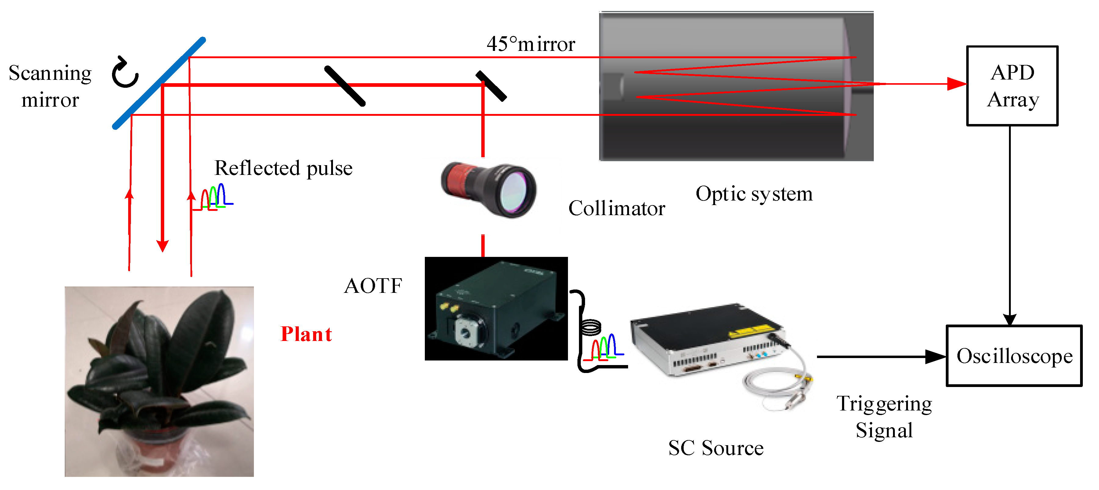
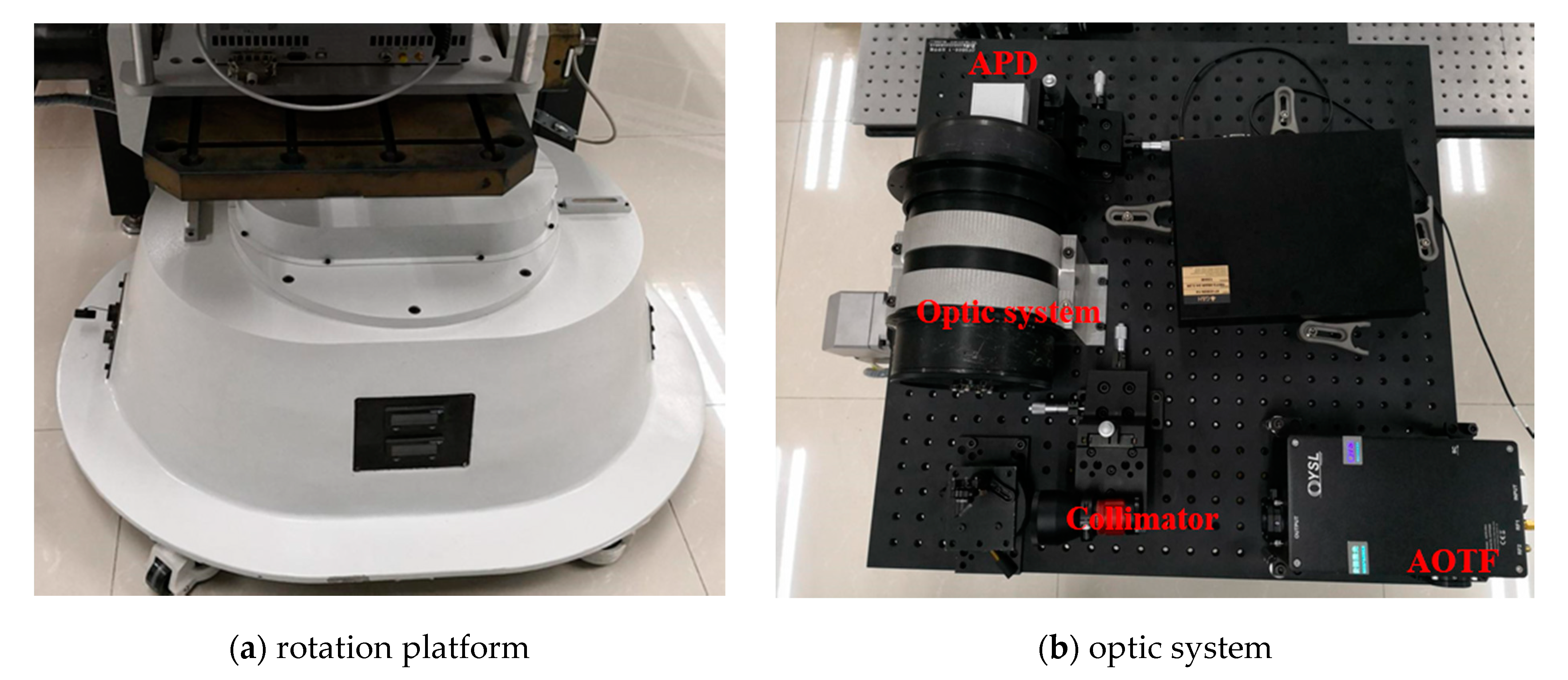
The system component and the working flow of the employed AOTF-HSL are presented in Figure 1; hardware prototype of the designed AOTF-HSL and the employed 2D rotation platform are shown in Figure 2. The HSL is assembled with several indispensable components, including the SC source, the wavelength selecting device or filtering component, the optical system, the reflected laser pulse detection module, and the data sampling and storing device. Specifications and particulars of these essential parts are given in detail as follows:

Figure 1.
Architecture and working flow of the employed AOTF-HSL.
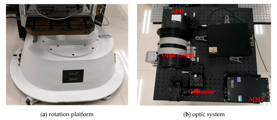
Figure 2.
A 2D rotation platform and the AOTF-HSL hardware prototype.
- (1)
- the first component is the laser source. In this HSL, the SC source is employed for generating “white” laser pulse, and the spectral band ranges from approximately 450 nm to 2500 nm [22];
- (2)
- the second component is the wavelength selecting or filtering device. After the laser source emitting the supercontinuum laser beam, a wavelength selecting device is installed after it for filtering the passing laser beam; in this HSL design, an AOTF is utilized as the wavelength selection device, and more specifications or parameters of the AOTF are available in our previously published paper [22]; additionally, after the wavelength selecting operation, a collimator is employed for guaranteeing the collimation of the laser beam;
- (3)
- the third component is the optical system, which steers the laser beam to the target and collects the reflected laser pulse from the target. The reflected pulse is detected by a silicon-based avalanche photodiode (APD). The data are then sampled by a connected high-speed oscilloscope (20 G per second), and the spectral reflectance is derived from the collected raw reflected waveform signals.
In this HSL, the ranging information is acquired by counting the time difference between the emitted laser pulse and the reflected laser pulse, and the spectral information is then extracted from the intensity, which is the maximum value of the collected raw waveforms [22]. Angular resolution of the HSL is 0.5 degree, the spectral resolution is 10 nm (500~1000 nm), and the range resolution is 3 cm (sampling frequency 5 GHz).
2.2. Vegetation Indexes and Parameters
In view of the demand of indicating the vegetation growth status in the precision agriculture, seven general vegetation spectral parameters related to different biochemical contents are employed for evaluating the HSL capacity in vegetation parameters extraction, specifically, the water index (WI), normalized difference vegetation index (NDVI), green normalized difference vegetation index (GNDVI), vegetation terrestrial chlorophyll index (TCI), normalized difference red edge index (NDREI), ratio vegetation index (RVI) and fluorescence ratio index (FRI) [26,27,28,29,30,31]. Equations of these spectral parameters are given by:
(1) Water index
where WI is sensitive to vegetation water content. The calculation is shown in the Equation (1). and are the spectral reflectance values at the corresponding wavelengths [26,32].
(2) Normalized difference vegetation index (NDVI)
where NDVI is an import indicator to reflect the vegetation growth and nutrition information. This index is capable of indicating the crop’s demand for nitrogen. Equation (2) presents the NDVI determination; the and are the spectral reflectance values employed in the calculation [27].
(3) Green normalized difference vegetation index (GNDVI)
where GNDVI is related to the leaf area index (LAI), and the equation is listed as Equation (3). and are the spectral reflectance values [27].
(4) Vegetation terrestrial chlorophyll index (TCI)
where TCI is sensitive to chlorophyll content; higher TCI value means more chlorophyll content. The TCI calculation is as Equation (4); , and are the corresponding reflectance values [28].
(5) Normalized difference red edge index (NDREI)
where NDREI is also related to the chlorophyll content in Equation (5); and are the spectral reflectance values at 750 nm and 705 nm wavelength [29].
(6) Ratio vegetation index (RVI)
where RVI is also related to the nutrition elements in vegetation [30].
(7) Fluorescence ratio index (FRI)
where FRI is the related to photosynthesis and chlorophyll fluorescence [31].
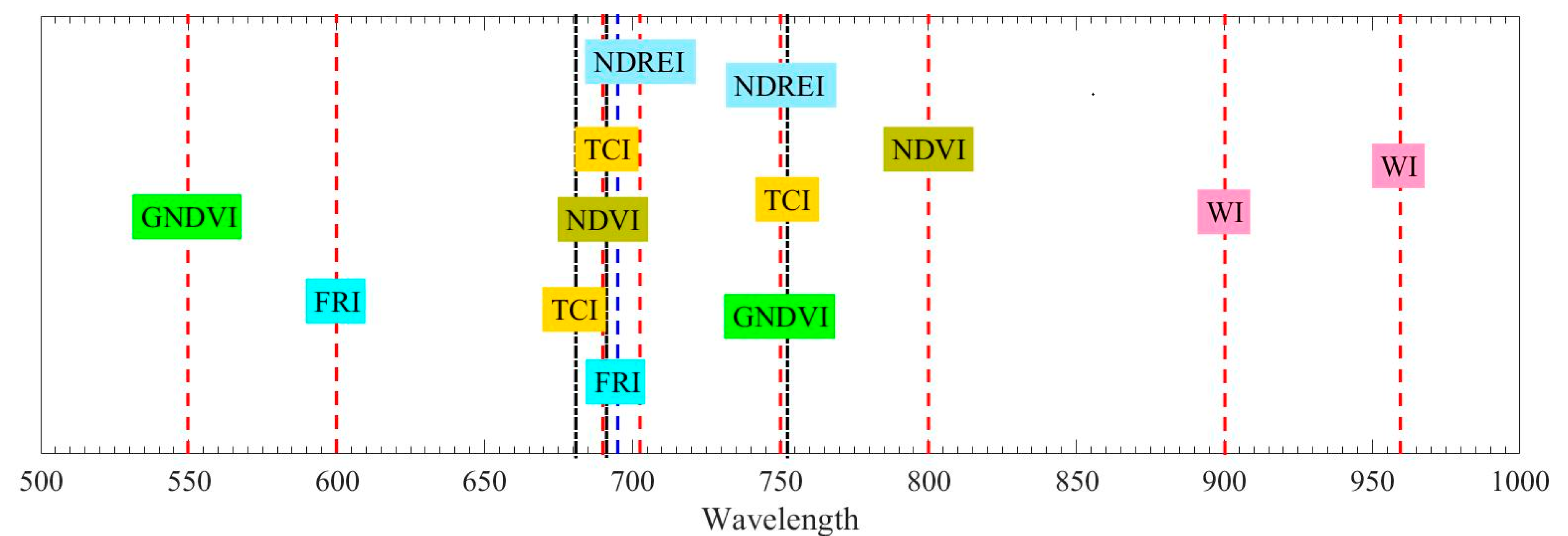
Table 2 and Figure 3 summarize the corresponding spectral wavelength of the spectral profiles employed in determining the vegetation spectral indexes. Figure 2 presents the spectral wavelength distribution totally; spectral profiles from twelve different spectral wavelengths covering 500–1000 nm are necessary for above vegetation spectral indexes calculation. It is impractical to combine twelve different single wavelength laser sources together to obtain the needed spectral profiles at a time. In addition, it is hard to guarantee all the laser beams from different laser sources are pointing to the same part of the target. The SC-based HSL is a more preferable and practical solution for this application.
Table 2.
Vegetation parameters.

Figure 3.
Corresponding wavelength of the spectral profiles employed in the determination of the indexes.
3. Laser Radiation Model
In the Section 2, equations of the spectral indexes are listed. However, for the HSL laser-reflected intensities, they are related to the laser incident angle and the materials of the target surface. Therefore, in this section, based on the laser intensity model, the spectral indexes considering the laser incident angle are analyzed and presented. Section 3.1 presents the basic model of the laser intensity, and the Section 3.2 presents the analysis of the spectral indexes considering the laser incident angle.
3.1. Laser Intensity Model
After reviewing the literatures [26,27], LiDAR intensity are influenced majorly by laser-beam-transmitting distance, incident angle, and reflectively of the target surface. Laser radiation model considering above factors is given by:
where denotes the received power of the reflected laser pulse, denotes the power of the transmitted laser pulse, denotes the transmitting distance of the laser pulse, denotes the reflectivity, denotes the solid scattering angle, denotes the receiver aperture, denotes the transmitted laser beam bandwidth, and denotes the laser pulse incident angle to the target surface.
3.2. Spectral Parameters Extraction Using Whiteboard as Reference
We divide these equations into three formulas: “(A − B)/(A + B)”, “A/B”, and “1/B”.
- (a)
- Spectral Parameters with “(A − B)/(A + B)” formula
Spectral parameters (SP) with “(A − B)/(A + B)” style is written as:
where the and are the spectral profiles at the wavelength and , respectively. Assume that the laser intensities from the target and whiteboard at are and .
The HSL laser intensities (LI) measuring the target and the whiteboard can be written as follows:
where the superscript “T” means the measurements from the target, the superscript “W” means the measurements from the whiteboard, the subscript and refers to the spectral wavelength, and means the incident angle of the laser pulse. With above assumptions, spectral profiles and can be written as:
Then, substituting the Equations (14) and (15) to the Equation (9), and Spectral Parameters with “(A − B)/(A + B)” formulas can be written as:
In HSL, and are established, and the calculation can be written as:
- (b)
- Spectral Parameters with “A/B” formulas
Spectral parameter (SP) with “A/B” style is written as:
Substituting the Equations (14) and (15) to the Equation (19), the spectral parameters with “A/B” style is written as:
Similarly, in HSL, and are established, and the calculation can be written as:
4. Results
In view of the demands of the precision agriculture, three experiments were carried out in this section for assessing the HSL-based spectral profiles acquirement, spectral parameters extraction, and vegetation classification. In the first experiments, two different plants, Dracaena (Dracaena angustifolia) and Aloe (Aloe arborescens Mill) with both green and yellow leaves, and another two different plants, Rubber tree (Ficus elastica Roxb. ex Hornem) and Radermachera (Radermachera hainanensis Merr) with only green leaves, were measured by the AOTF-HSL (plants employed in this experiment are the same as that in our previous paper; the figures of these plants can be found in the literature [22]). The experiments were carried out indoors under controlled environment for collecting the spectral profiles. The plant was placed approximately 17 m in front of the HSL. Since the spectral pulse intensity was related to the incident angle, the laser pulse was perpendicularly pointed to the surface of the vegetation leaves. Apart from the AOTF-HSL, a passive SVC spectrometer (SVC HR-1024) was employed for acquiring the spectral profiles of the above four different plants. The extracted vegetation spectral indexes from the HSL were compared with that from a passive SVC spectrometer for evaluating the difference, which aimed to assess the feasibility of using HSL to extract the above spectral indexes; then, the results of the green and yellow leaves were compared for validating the differences of the selected vegetation spectral indexes, which could demonstrate the effectiveness of the HSL in vegetation growth status indication and vegetation physiological changes detection.
In addition, in the second experiment, another sixteen different leaves were also measured by the AOTF-HSL. A multi-label SVM was designed and employed to classify the leaves. Based on the assessing results of the vegetation parameters, six different spectral parameters were calculated and utilized as the input features of the SVM classifier. The classification results were presented, analyzed, and discussed for demonstrating the great AOTF-HSL potential in vegetation classification and mapping.
Finally, in the third experiment, Fraxinus velutina, Eucommia ulmoides, and Prunus triloba Lindl green leaves and Fraxinus velutina yellow leaf were measured by the HSL and an ASD FieldSpec 4 spectrometer (ASD© FieldSpec 4). The spectral profiles from the spectrometer were employed as the reference to evaluate the results from the HSL. These leaves were measurement by the HSL at different incident angles (0°, 10°, 20°, 30°, 40°, 50°, 60°, 70°, and 80°). The laser pulse incident angle was set by a compass. Distance information and spectral information were obtained at different incident angles. Normalized difference vegetation index (NDVI) and water index (WI) were employed as the representative parameters of the “(A − B)/(A + B)” and “A/B” styles. NDVI and WI results were calculated using the spectral profiles collected at different incident angles.
4.1. Experiment #01—Spectral Indexed Results Comparison
4.1.1. Green Leaf Results
WI extraction results for the employed four different plants with green leaves are presented in Table 3. It was notable that all the WI values of the four different green leaves were all below one, and the differences between HSL and SVC spectrometer results were all below 5%. Besides, the difference equation was as the following Equation (11):
where the was the extracted parameters from the HSL measurements, and the was the corresponding parameters from the SVC spectrometer spectral profiles.
Table 3.
Spectral indexes results comparison.
We could observe that the NDVI from HSL and SVC spectrometer performed quite similarly with the results listed in Table 3. The Dracaena green leaf difference was below 1%, which was the minimum difference among the four green leaves. By contrast, the Aloe green leaf had the maximum difference, and the difference value was 3.8%. In aspects of the GNDVI results, the Dracaena and Aloe green leaves’ difference were more significant than 5%. The Rubber plant and Radermachera green leaves’ difference between HSL and SVC spectrometer were all below 5%.
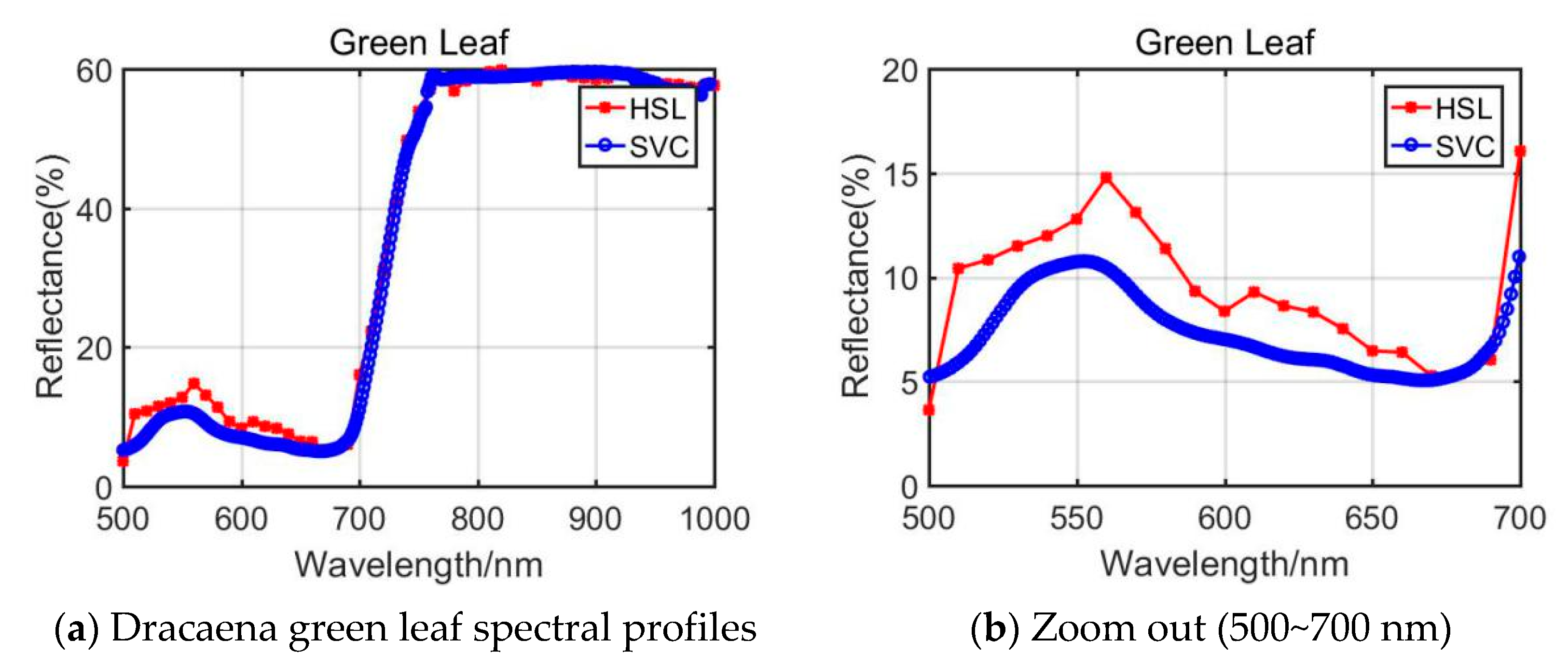
By comparing the results difference between NDVI and GNDVI, the GNDVI yielded a slightly bigger difference. Through analyzing the NDVI and GNDVI calculation equations (Equations (2) and (3)) and the spectral profiles plotted in Figure 4, we observed that the spectral reflectance at 750 nm derived from the HSL on Aloe green leaf of the HSL was larger than that of SVC, while they had similar reflectance at 550 nm. This accounted for the phenomenon that Aloe green leaf yielded a larger difference in NDVI and GNDVI parameter extraction.

Figure 4.
Dracaena green leaf spectral profiles.
The rest of the four parameters, TCI, NDREI, RVI, and FRI, were related to the vegetation biochemical and biological contents. TCI, NDREI, RVI, and FRI from HSL and SVC spectrometer spectral profiles are listed in Table 3. It could be observed that the HSL and SVC yielded more significant differences compared with previous WI, NDVI, and GNDVI parameters results.
For the Dracaena green leaf, the difference of the TCI, NDERI, RVI, and FRI was larger; only NDERI was below 20%. As listed in Section 2, the spectral profiles covering 500~700 nm were included in the calculation of the TCI, NDERI, RVI, and FRI values, and the reflectance values from HSL and SVC were slightly different. The spectral profiles comparison is shown in Figure 4a,b. As presented in these figures, compared with the spectral profiles of 700~1000 nm, the 500~700 nm spectral reflectance was quite different.
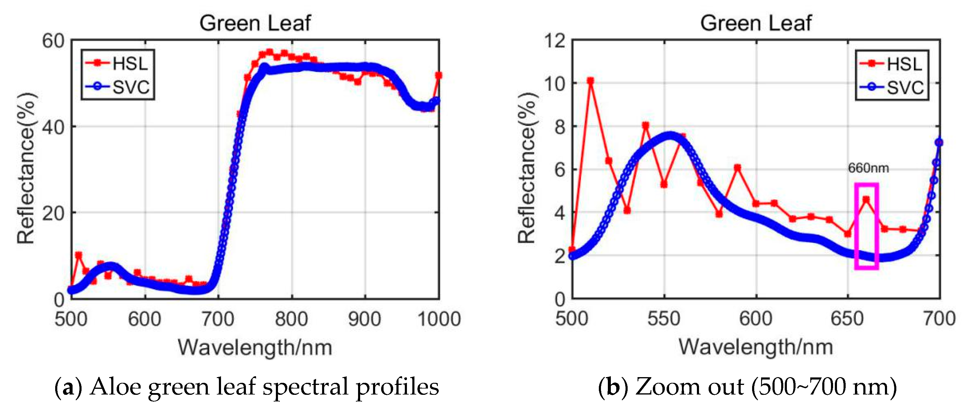
In aspects of Aloe green leaf results, the RVI parameters from HSL and SVC show clear difference. As plotted in Figure 5b, the reflectance values (500~700 nm) from HSL and SVC were different, and HSL spectral values were larger than SVC. Especially different was the spectral profiles’ difference at the wavelength at 660 nm (marked with a pink rectangle in Figure 5b); this would affect the RVI index determination results.
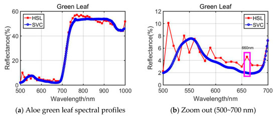
Figure 5.
Aloe green leaf spectral profiles.
From the presented Rubber tree’s and the Radermachers’s spectral curves in Figure 6 and Figure 7, we could observe that the results were also affected by the difference of the 500~700 nm spectral profiles reflectance. Among them, the Radermachera yielded the best similarity in the 500~700 nm spectral reflectance values between HSL and SVC.
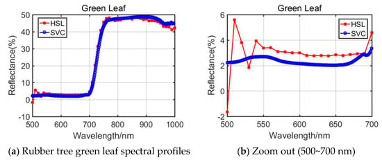
Figure 6.
Rubber tree green leaf spectral profiles.
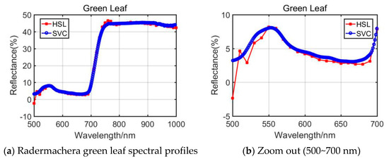
Figure 7.
Radermachera green leaf spectral profiles.
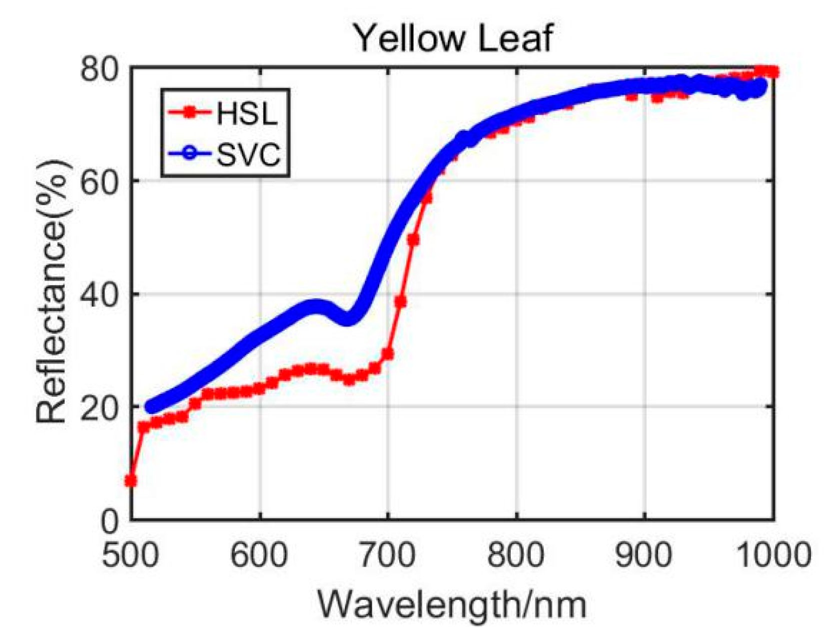
4.1.2. Yellow Leaf Results Analysis
Previously, Section 3.1 listed the green leaves’ results of these vegetation spectral indexes, and the following Table 4 shows the results from the Dracaena yellow leaf and the Aloe yellow leaf. Additionally, the green leaves’ results are listed in the Table 4 for comparison. Among the yellow leaves results, the difference was unsatisfactory apart from the Dracaena yellow leaf WI and RVI index results. The spectral profiles from the HSL and SVC spectrometer are presented in Figure 8 and Figure 9. Compared with green leaf results, the curves were relatively distinctive due to the fact that the HSL laser pulse footprint diameter was approximately 1 cm on the target with these settings. The sampled area on the yellow leaves had huge difference between two apparatuses; this might also be the reason that the spectral profiles collected by the HSL were steeper at red edge, as shown in Figure 8 and Figure 9. Furthermore, the yellow leaves had uneven distributions of the biochemical and biological contents in the covered area of the footprint.
Table 4.
Spectral indexes results comparison.
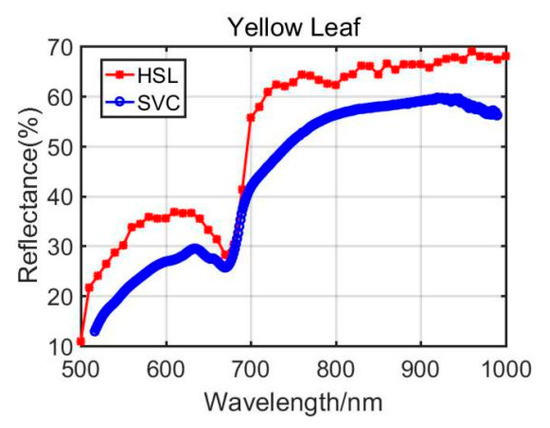
Figure 8.
Dracaena yellow leaf spectral profiles.

Figure 9.
Aloe yellow leaf spectral profiles.
Through analyzing the difference of the parameters between green and yellow leaves, the indexes demonstrated similar changing trends. For instance, the yellow leaf WI index had a minor increase due to the lower water content in yellow leaves. The NDVI values also performed a dramatic decrease since the yellow leaves had lower chlorophyll. The similar changing trend could be observed from the results of other vegetation spectral indexes. Results from the comparison between green and yellow were able to give positive support for the feasibility study of using the HSL in vegetation spectral indexes estimation, determination, and growth status indicating.
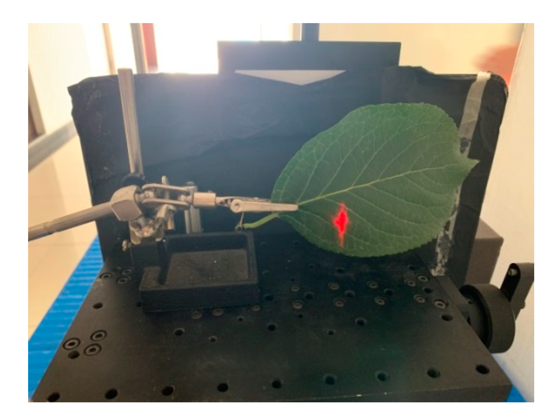
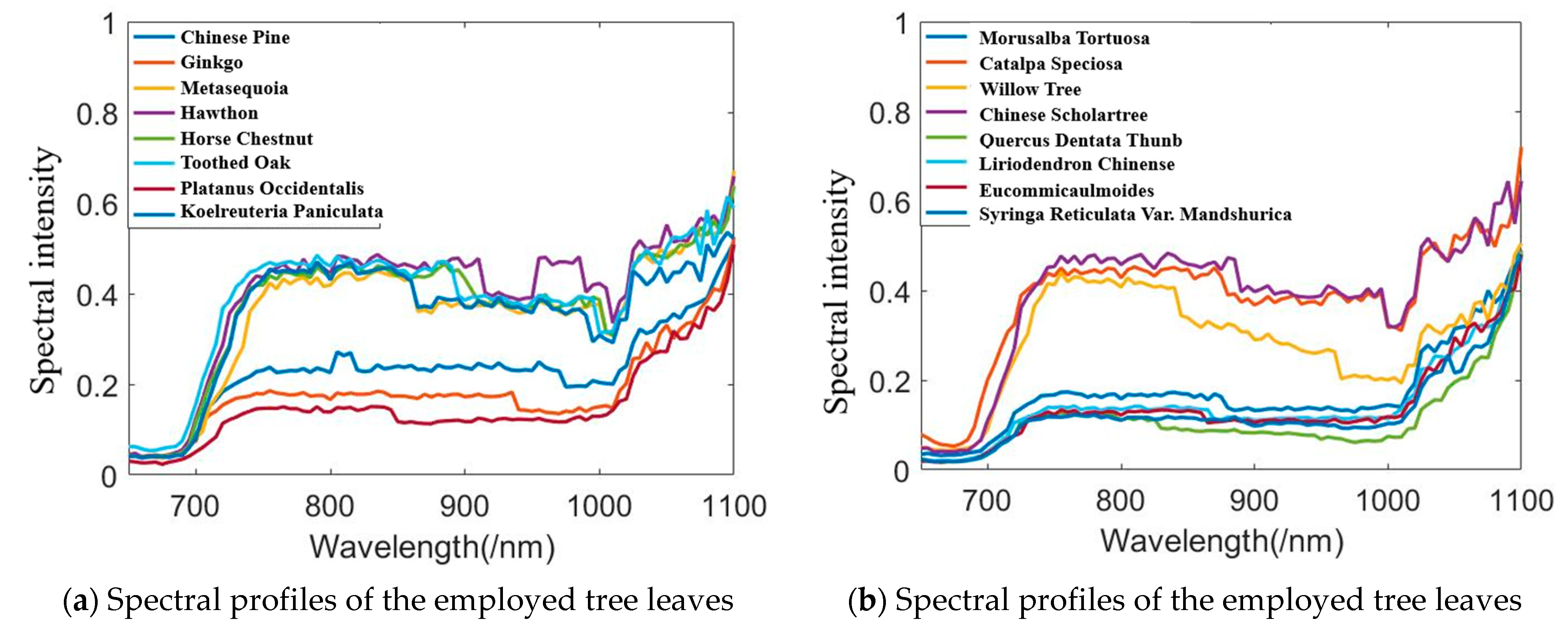
4.2. Experiment #02—Vegetation Leaves Classification
Figure 10 presents an example of scanning the leaf with HSL. The red point was the footprint of the HSL laser pulse. The collected spectral profiles of the sixteen different leaves are presented in Figure 10; the spectral profiles plotted in Figure 11a included the Chinese pine (Juniperus rigida), Ginkgo (Ginkgo biloba), Metasequoia (Metasequoia glyptostroboides), hawthorn (Crataegus pinnatifida), Horse chestnut (Aesculus hippocastanum), Toothes oak (Quercus), Platanus occidentalis, and Koelreuleria Paniculata. The spectral profiles of the left eight different leaves in Figure 11b included Morusalba Tortuosa, Catalpa speciose, Willow tree (Salix), Chinese scholartree (Styphnolobium japonicum), Quercus dentate Thunb, liriodendron chinense (Chinese Tulip Tree), Eucommiaulmoides, and Syringa reticulate var. mandshurica. Limited by the HSL working spectral coverage, the spectral profiles presented in Figure 11 were sampled ranging from 650 nm to 1100 nm. Another spectral parameter set (NDVI, SR, NDVI705, VOG, WI, and RVI) was extracted and presented. SR, NDVI705, and VOG were the new parameters different from that of the first experiment. The definitions and explanations were listed as the following Equations (23)–(25).

Figure 10.
Spectral profiles collection in the lab.
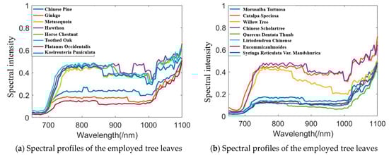
Figure 11.
Spectral profiles of the leaves.
(1) Simple ratio Iidex (SR)
where and are the spectral reflectance of the wavelength 800 nm and 680 nm.
(2) Vogelmann index (VOG)
where and are the spectral reflectance of the wavelength 800 nm and 680 nm.
(3) Normalized difference vegetation index (NDVI705)
Similarly, and are the spectral reflectance at 750 nm and 705 nm wavelength.
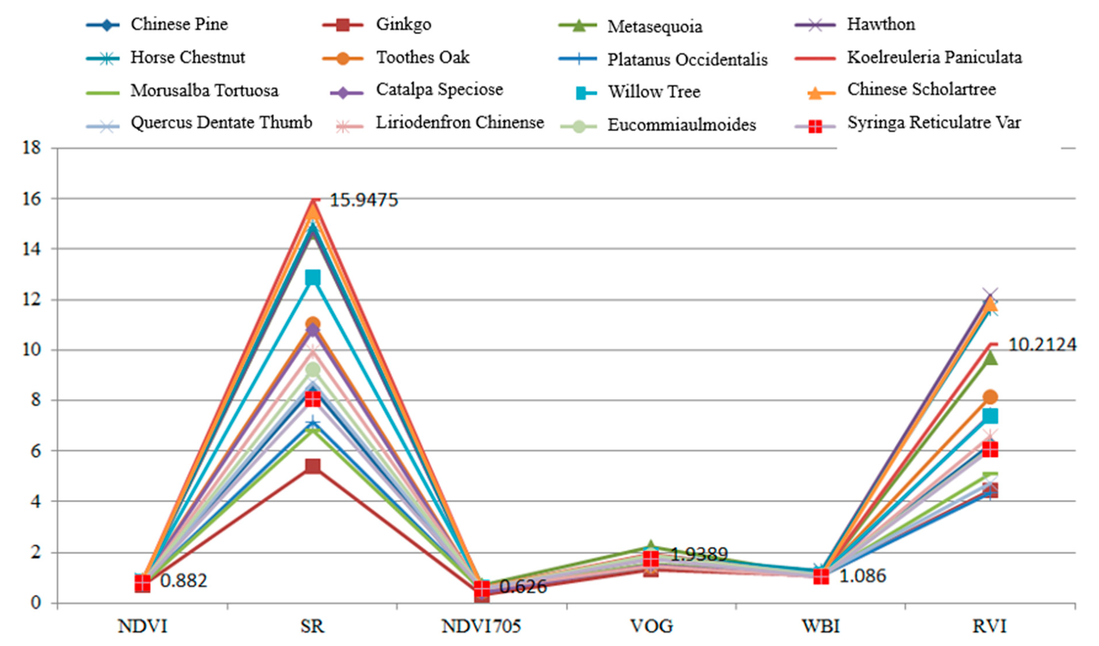
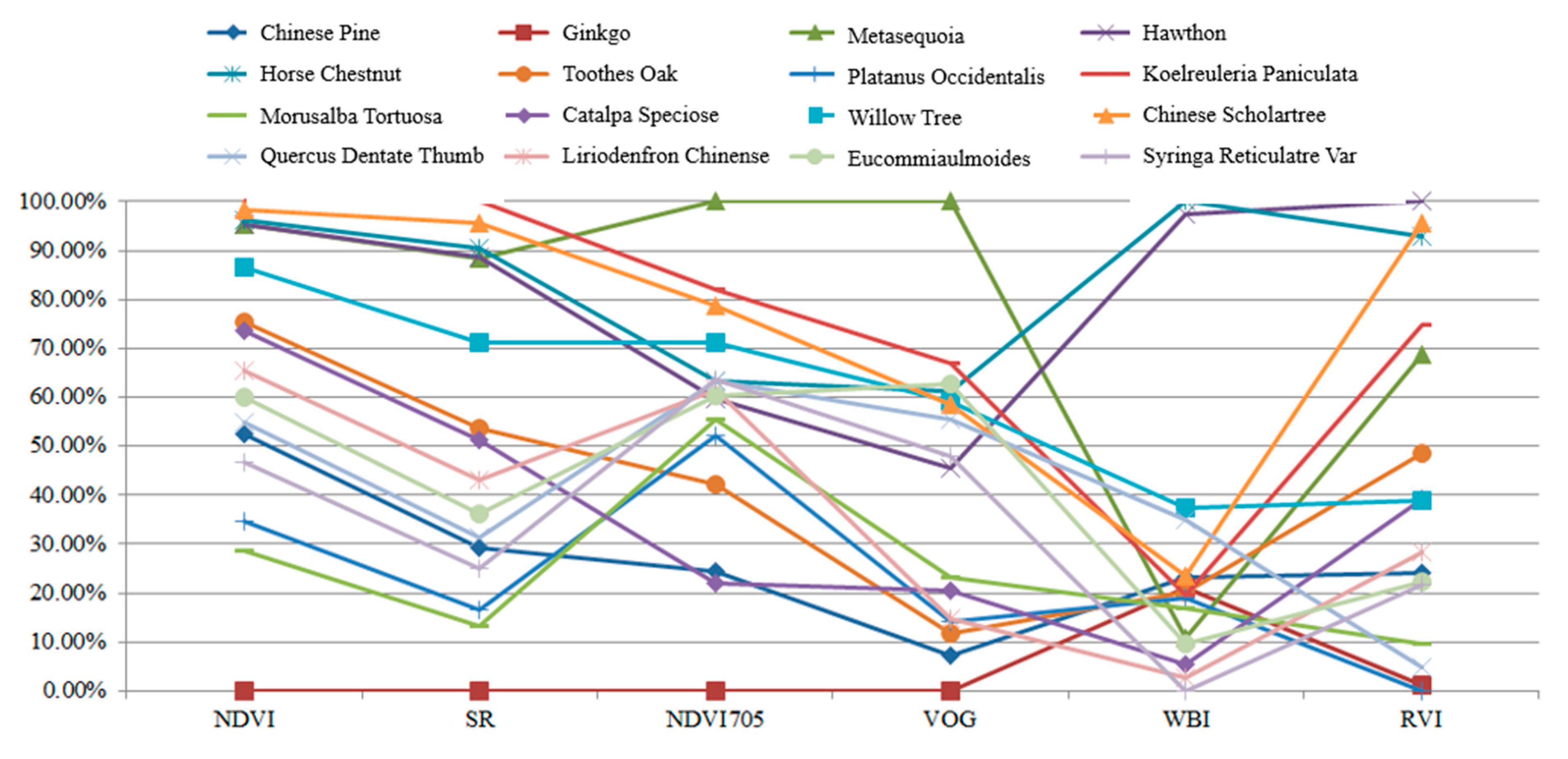
Table 5 presents the calculation results of the spectral indexes for these leaves. In this experiment, each leaf was scanned by the HSL four times. The spectral profiles presented in Figure 11 were the average values of the four-time measurements. Parameters results listed in Table 5 were also calculated using the averaged spectral profiles measurements. Figure 12 plots the parameters of the employed sixteen leaves. Basically, the parameters of these leaves were distinctive, which indicated that these leaves were divisible using these spectral parameters as the feature vector.
Table 5.
Vegetation spectral indexes results.
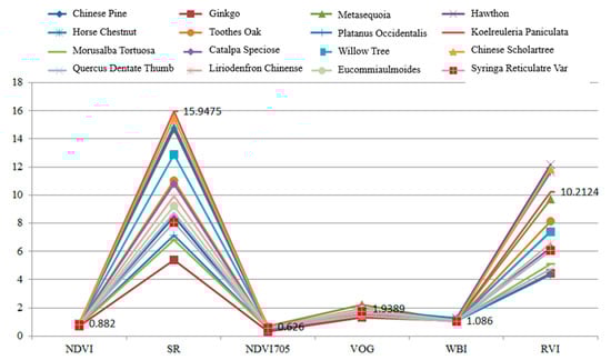
Figure 12.
Parameters of the employed leaves.
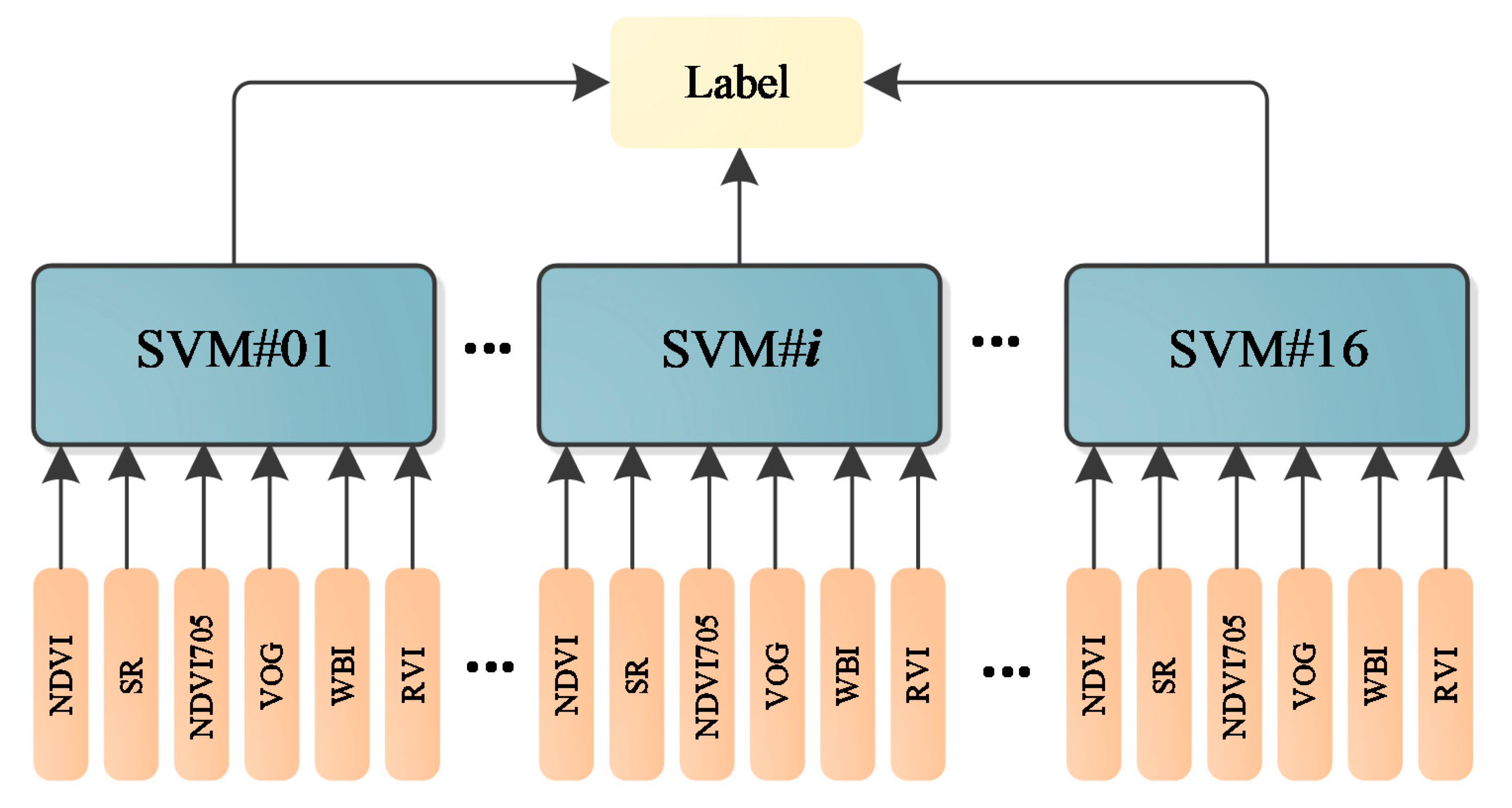
As presented in Figure 12, different parameters are not in the same orders of magnitude. Therefore, before employing the parameters in the classification, the normalization of the parameters is necessary. The normalized parameters of these leaves are plotted in Figure 13. Compared with Figure 12, the parameters are more balanced. The feature vector composed by the normalized six parameters is employed as the input vector of the SVM classifier. Since we have sixteen different leaves, a SVM classifier with multiple labels was designed and its structure is presented in Figure 14.
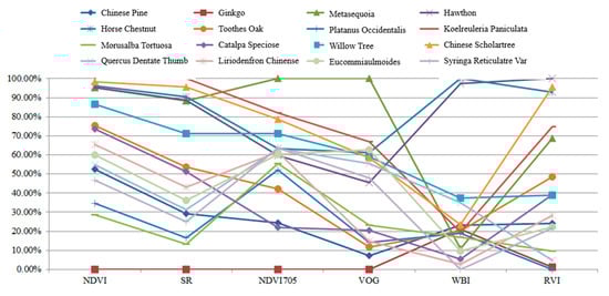
Figure 13.
Normalized parameters of the employed leaves.
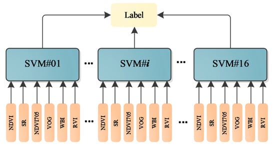
Figure 14.
The multi-label SVM classifier.
We scanned the leaves at different spectral wavelengths, and the spectral intensities from these wavelengths were randomly selected to generate more samples for training the classifier. For instance, we scanned these leaves at 750 nm eight times for each leaf; then, we randomly selected one measurement from the eight, and the same operation was conducted for other spectral wavelengths and leaf samples. Here, a training dataset was randomly selected from the first 50% of the datasets and the testing dataset was selected from the rest of the 50% of datasets. The training and testing dataset both contained 1000 samples, which was randomly selected from the collected dataset. Table 6 lists the classification accuracy of the sixteen leaves using the designed multi-label SVM classifier. All the classification accuracies could reach 100% with the dataset. No SVM parameters optimization was carried out; the multi-label SVM classifier was built on the default SVM in MATLAB. The kernel function was revised from “linear” to “RBF”.
Table 6.
Vegetation parameters results.
4.3. Experiment #03—Influence of the Incident Angle Analysis on Spectral Indexes Results
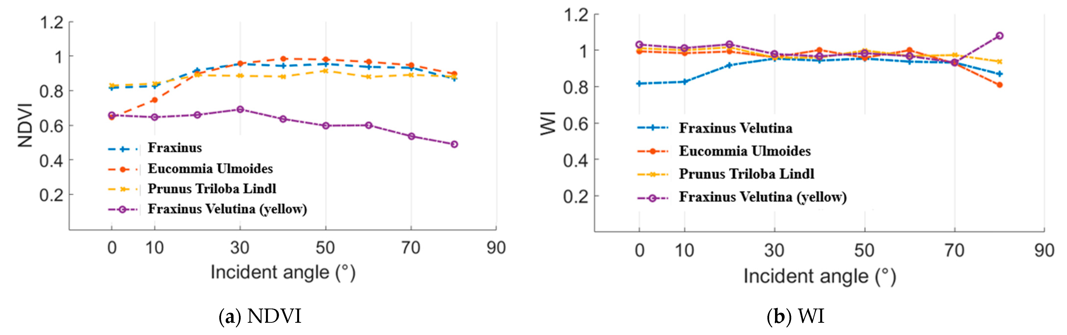
In this experiment, normalized difference vegetation index (NDVI) and water index (WI) were employed as the representative parameters of the “(A − B)/(A + B)” and “A/B” styles. NDVI and WI results of the Fraxinus velutina, Eucommia ulmoides, and Prunus triloba Lindl green leaves and Fraxinus velutina yellow leaf are presented in the Figure 14. A 100% whiteboard was employed as the reference to calculate these NDVI and WI results. As analyzed in the Section 2.2, the incident angle had no influence on the NDVI and WI results. In Figure 15, the incident angles were 0°, 10°, 20°, 30°, 40°, 50°, 60°, 70°, and 80°. The distance remained the same while measuring the whiteboard and these leaves. It could be seen that the NDVI and WI values varied at a limited range, which demonstrated that the incident angle almost had no influence on the NDVI and WI results.
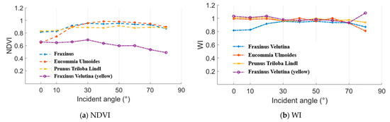
Figure 15.
NDVI and WI results.
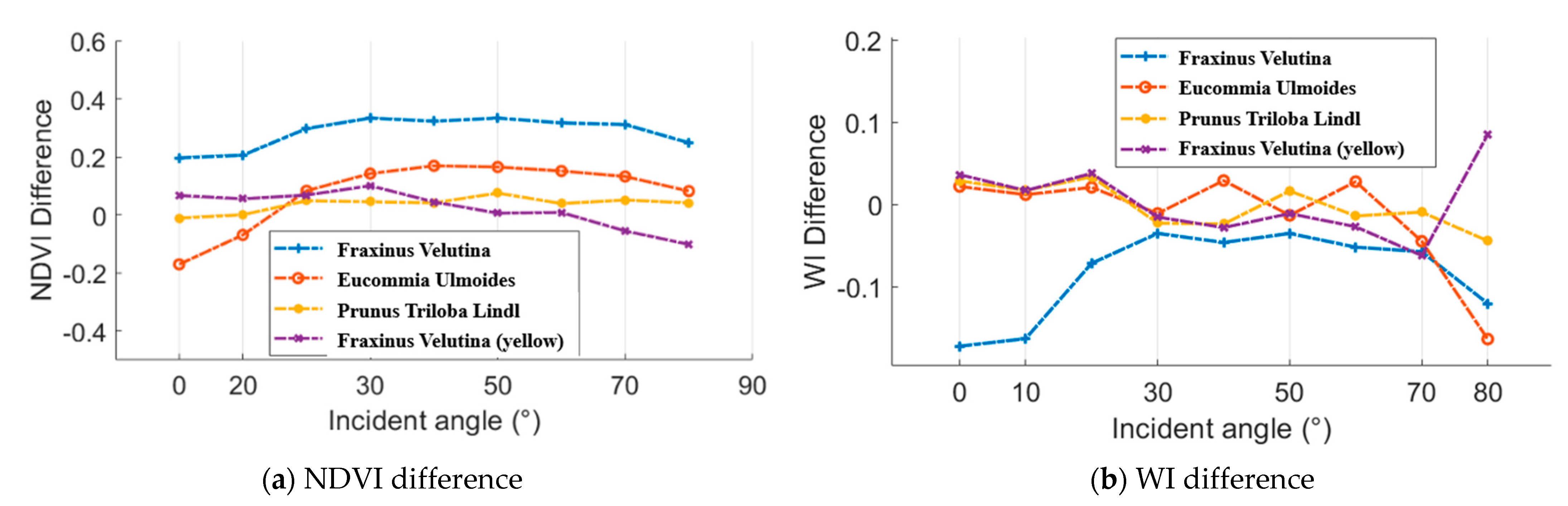
As aforementioned, an ASD FieldSpec 4 spectrometer was employed to collect the spectral profiles, which could be regarded as the reference. Figure 16 presents the difference results between the spectral parameters from the HSL and spectrometer. In aspects of the NDVI difference, Eucommia ulmoides and Prunus triloba Lindl green leaves and Fraxinus velutina yellow leaf NDVI difference were smaller than 0.2 at all the selected incident angles. In addition, the most of the WI difference results were smaller than 0.1.
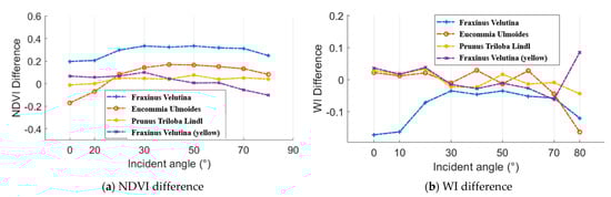
Figure 16.
NDVI and WI difference between the results from the HSL and spectrometer.
5. Discussion
Part of the green leaves’ results demonstrated distinctive differences between the HSL and the SVC spectrometer (Table 3), i.e., the RVI of the Aloe green leaf. Difference of the reflectance values (500~700 nm) from HSL and SVC brought about the larger difference in the spectral indexes. We thought the following two reasons could be summarized to account for why the spectral reflectance (500~700 nm) difference affected the green leaves results to such a great extent.
- (1)
- The first reason was that the vegetation yielded low reflectivity in the spectral band 500~700 nm, and the small changes or difference would be relatively large in proportion;
- (2)
- The second reason was that the reflectance of 500~700 nm was employed as the denominator for determining the parameters. For instance, the WI index demonstrated high similarity since the employed spectral wavelength had high reflected intensities; small difference or fluctuations in spectral reflectance was relatively a small proportion; in fact, HSL and SVC yielded minor difference within the 700 nm~1000 nm spectral wavelength for the four green leaves, but the high reflectivity yielded a difference in just a small proportion and almost had no influence on the parameters results.
As presented in the Figure 15 and Figure 16, the NDVI and WI results were not exactly the same; there were some fluctuations. We thought the following reasons might account for this phenomenon:
- (1)
- The power of the received laser pulse was affected by many factors. In Figure 3, these NDVI and WI results were calculated with the distance fixed and the incident angle changed. As analyzed in Equations (18) and (21), some other factors also affected the NDVI and WI results.
- (2)
- The NDVI and WI results difference between the HSL and spectrometer varied at different incident angles, which might be caused by the noises contained in the HSL raw waveforms. Here, no de-noising or calibration operation conducted for the raw HSL measurements was carried out.
Although the above work demonstrates the ability of the AOTF-HSL, we thought the following limitations were worthy of further investigation:
- (1)
- For the green leaves spectral profiles, we found that low reflectivity spectral bands (500~700 nm) demonstrated comparatively different spectral reflectance values (Figure 4b, Figure 5b, Figure 6b and Figure 7b); these fluctuations of the AOTF-HSL spectral profiles affected the difference; the fluctuations might be caused by the noise contained in the raw measurements in the HSL. A filtering scheme (Gaussian fitting) or better HSL setting-up might be effective for bettering the results.
- (2)
- The HSL employed in this paper owned a 10 nm spectral resolution; it was comparatively better than previous HSL, but the spectral resolution of SVC spectrometer was better than 10 nm, and the low spectral resolution partially accounted for the AOTF-HSL spectral profiles fluctuations (Figure 4b, Figure 5b, Figure 6b and Figure 7b); it was of great significance for developing HSL with finer resolution, and it would bring new, interesting results for vegetation spectral indexes determination.
- (3)
- The spectral data in this experiment were collected at the fixed distance, and a proper calibration method or solution was essential for calibrating the HSL while collecting the spectral profiles with different distance and incident angles. In other words, the incident angle effect on the HSL should be investigated.
- (4)
- In this paper, the HSL just scanned one point for each leaf, and the laser beam footprint was comparatively large. For 3D imaging of the vegetation spectral indexes distribution, HSL with narrow field of view resulting in higher spatial resolution was of great significance for extending the application.
- (5)
- Based on this HSL, a classic multi-label SVM classifier was designed and employed for tree leaves classification; a simple classifier could reach satisfactory classification accuracy. We thought two major reasons might account for these phenomena: the experiment was carried out in the lab with a controlled environment with almost no external factors that could affect the HSL collecting the spectral profiles of the leaves; the leaves employed in the experiment are all green leaves, which has uniform distribution of the biological contents.
- (6)
- Calibration of the HSL should be carried out and some intrinsic and extrinsic factors should be modeled, which was helpful to improve the HSL measurements. There must be noises contained in the HSL raw waveforms; appropriate de-noising methods should be investigated.
6. Conclusions
This paper conducts a comprehensive assessment of the AOTF-HSL in vegetation spectral indexes extraction and growth stratus indicating, which is of significance for extending HSL applications in precision agriculture. The findings of this paper are summarized as:
- (1)
- This paper presented a practical HSL design suitable for precision agriculture applications.
- (2)
- The consistency of green leaves spectral indexes results extracted from both the SVC and the HSL demonstrates that the AOTF-HSL with current settings was feasible and executable for vegetation spectral profiles acquirement.
- (3)
- This paper investigated the incident angle effect on the spectral indexes determination; we found that the incident angle had no influence on the spectral parameters with “(A − B)/(A + B)” and “A/B” styles.
Author Contributions
Methodology, C.J. and Y.C.; software, C.J.; validation, Y.C. and W.L., and H.W.; formal analysis, H.S.; writing—original draft preparation, J.J., C.J. and Y.C.; writing—review and editing, C.J., Y.C., W.L., F.Y., H.W., E.P., J.H, P.H., and S.W.; supervision, Y.C, J.H.; project administration, Y.C. and J.H.; funding acquisition, Y.C. and J.H. All authors have read and agreed to the published version of the manuscript.
Funding
This research was financially supported by the Ultrafast Data Production with Broadband Photodetectors for Active Hyperspectral Space Imaging (336145)”, Forest-Human-Machine Interplay—Building Resilience, Redefining Value Networks, and Enabling Meaningful Experiences (UNITE), (337656) and Strategic Research Council project “Competence-Based Growth Through Integrated Disruptive Technologies of 3D Digitalization, Robotics, Geospatial Information, and Image Processing/Computing—Point Cloud Ecosystem (314312). Additionally, Chinese Academy of Science (181811KYSB20160113, XDA22030202), Beijing Municipal Science, and Technology Commission (Z181100001018036), Shanghai Science and Technology Foundations (18590712600), and Jihua lab (X190211TE190) and Huawei (9424877).
Informed Consent Statement
Not applicable.
Data Availability Statement
The data presented in this study are available on request from the corresponding author.
Acknowledgments
We acknowledge any support given by all institue and projects, and we also acknowledge everyone’s assistance.
Conflicts of Interest
The authors declare no conflict of interest.
References
- Asra, G. Theory and Applications of Optical Remote Sensing; Asrar, G., Ed.; Wiley: New York, NY, USA, 1989. [Google Scholar]
- Ceccato, P.; Gobron, N.; Flasse, S.; Pinty, B.; Tarantola, S. Designing a spectral index to estimate vegetation water content from remote sensing data: Part 1: Theoretical approach. Remote Sens. Environ. 2002, 82, 188–197. [Google Scholar] [CrossRef]
- Turner, W.; Spector, S.; Gardiner, N.; Fladeland, M.; Sterling, E.; Steininger, M. Remote sensing for biodiversity science and conservation. Trends Ecol. Evol. 2003, 18, 306–314. [Google Scholar] [CrossRef]
- Verrelst, J.; Camps-Valls, G.; Muñoz-Marí, J.; Rivera, J.P.; Veroustraete, F.; Clevers, J.G.; Moreno, J. Optical remote sensing and the retrieval of terrestrial vegetation bio-geophysical properties—A review. ISPRS J. Photogramm. Remote Sens. 2015, 108, 273–290. [Google Scholar] [CrossRef]
- Nevalainen, O.; Hakala, T.; Suomalainen, J.; Mäkipää, R.; Peltoniemi, M.; Krooks, A.; Kaasalainen, S. Fast and nondestructive method for leaf level chlorophyll estimation using hyperspectral LiDAR. Agric. For. Meteorol. 2014, 198, 250–258. [Google Scholar] [CrossRef]
- Zhou, H.; Chen, Y.; Feng, Z.; Li, F.; Hyyppä, J.; Hakala, T.; Karjalainen, M.; Jiang, C.; Pei, L. The comparison of canopy height profiles extracted from Ku-band profile radar waveforms and LiDAR data. Remote Sens. 2018, 10, 701. [Google Scholar] [CrossRef] [Green Version]
- Danson, F.M.; Gaulton, R.; Armitage, R.P.; Disney, M.; Gunawan, O.; Lewis, P.; Pearson, G.; Ramirez, A.F. Developing a dual-wavelength full-waveform terrestrial laser scanner to characterize forest canopy structure. Agric. For. Meteorol. 2014, 198, 7–14. [Google Scholar] [CrossRef] [Green Version]
- Eitel, J.U.; Höfle, B.; Vierling, L.A.; Abellán, A.; Asner, G.P.; Deems, J.S.; Mandlburger, G. Beyond 3-D: The new spectrum of lidar applications for earth and ecological sciences. Remote Sens. Environ. 2016, 186, 372–392. [Google Scholar] [CrossRef] [Green Version]
- Li, W.; Sun, G.; Niu, Z.; Gao, S.; Qiao, H. Estimation of leaf biochemical content using a novel hyperspectral full-waveform LiDAR system. Remote Sens. Lett. 2014, 5, 693–702. [Google Scholar] [CrossRef]
- Du, L.; Gong, W.; Shi, S.; Yang, J.; Sun, J.; Zhu, B.; Song, S. Estimation of rice leaf nitrogen contents based on hyperspectral LIDAR. Int. J. Appl. Earth Obs. Geogr. Inf. 2016, 44, 136–143. [Google Scholar] [CrossRef]
- Sun, J.; Shi, S.; Gong, W.; Yang, J.; Du, L.; Song, S.; Zhang, Z. Evaluation of hyperspectral LiDAR for monitoring rice leaf nitrogen by comparison with multispectral LiDAR and passive spectrometer. Sci. Rep. 2017, 7, 40362. [Google Scholar] [CrossRef]
- Jiang, C.; Chen, Y.; Wu, H.; Li, W.; Zhou, H.; Bo, Y.; Hyyppä, J. Study of a High Spectral Resolution Hyperspectral LiDAR in Vegetation Red Edge Parameters Extraction. Remote Sens. 2019, 11, 2007. [Google Scholar] [CrossRef] [Green Version]
- Suomalainen, J.; Hakala, T.; Kaartinen, H.; Räikkönen, E.; Kaasalainen, S. Demonstration of a virtual active hyperspectral LiDAR in automated point cloud classification. ISPRS J. Photogramm. Remote Sens. 2011, 66, 637–641. [Google Scholar] [CrossRef]
- Kaasalainen, S.; Lindroos, T.; Hyyppa, J. Toward hyperspectral lidar: Measurement of spectral backscatter intensity with a supercontinuum laser source. IEEE Geosci. Remote Sens. Lett. 2007, 4, 211–215. [Google Scholar] [CrossRef]
- Chen, Y.; Räikkönen, E.; Kaasalainen, S.; Suomalainen, J.; Hakala, T.; Hyyppä, J.; Chen, R. Two-channel hyperspectral LiDAR with a supercontinuum laser source. Sensors 2010, 10, 7057–7066. [Google Scholar] [CrossRef] [Green Version]
- Hakala, T.; Suomalainen, J.; Kaasalainen, S.; Chen, Y. Full waveform hyperspectral LiDAR for terrestrial laser scanning. Opt. Express 2012, 20, 7119–7127. [Google Scholar] [CrossRef]
- Vauhkonen, J.; Hakala, T.; Suomalainen, J.; Kaasalainen, S.; Nevalainen, O.; Vastaranta, M.; Hyyppä, J. Classification of spruce and pine trees using active hyperspectral LiDAR. IEEE Geosci. Remote Sens. Lett. 2013, 10, 1138–1141. [Google Scholar] [CrossRef]
- Li, W.; Niu, Z.; Sun, G.; Gao, S.; Wu, M. Deriving backscatter reflective factors from 32-channel full-waveform LiDAR data for the estimation of leaf biochemical contents. Opt. Express 2016, 24, 4771–4785. [Google Scholar] [CrossRef]
- Wang, Z.; Chen, Y.; Li, C.; Tian, M.; Zhou, M.; He, W.; Zhou, H. A Hyperspectral LiDAR with Eight Channels Covering from VIS to SWIR. In Proceedings of the IGARSS 2018–2018 IEEE International Geoscience and Remote Sensing Symposium, Valencia, Spain, 22–27 July 2018; pp. 4293–4296. [Google Scholar]
- Li, W.; Jiang, C.; Chen, Y.; Hyyppä, J.; Tang, L.; Li, C.; Wang, S.W. A Liquid Crystal Tunable Filter-Based Hyperspectral LiDAR System and Its Application on Vegetation Red Edge Detection. IEEE Geosci. Remote Sens. Lett. 2019, 16, 291–295. [Google Scholar] [CrossRef]
- Chen, Y.; Jiang, C.; Hyyppä, J.; Qiu, S.; Wang, Z.; Tian, M.; Bo, Y. Feasibility Study of Ore Classification Using Active Hyperspectral LiDAR. IEEE Geosci. Remote Sens. Lett. 2018, 99, 1–5. [Google Scholar] [CrossRef]
- Chen, Y.; Li, W.; Hyyppä, J.; Wang, N.; Jiang, C.; Meng, F.; Li, C. A 10-nm Spectral Resolution Hyperspectral LiDAR System Based on an Acousto-Optic Tunable Filter. Sensors 2019, 19, 1620. [Google Scholar] [CrossRef] [Green Version]
- Shao, H.; Chen, Y.; Yang, Z.; Jiang, C.; Li, W.; Wu, H.; Wang, S.; Yang, F.; Chen, J.; Puttonen, E.; et al. Feasibility Study on Hyperspectral LiDAR for Ancient Huizhou-Style Architecture Preservation. Remote Sens. 2020, 12, 88. [Google Scholar] [CrossRef] [Green Version]
- Shao, H.; Chen, Y.; Yang, Z.; Jiang, C.; Li, W.; Wu, H.; Wen, Z.; Wang, S.; Puttnon, E.; Hyyppä, J. A 91-Channel Hyperspectral LiDAR for Coal/Rock Classification. IEEE Geosci. Remote Sens. Lett. 2020, 17, 1052–1056. [Google Scholar] [CrossRef] [Green Version]
- Malkamäki, T.; Kaasalainen, S.; Ilinca, J. Portable hyperspectral lidar utilizing 5 GHz multichannel full waveform digitization. Opt. Express 2019, 27, A468–A480. [Google Scholar] [CrossRef]
- Peñuelas, J.; Pinol, J.; Ogaya, R.; Filella, I. Estimation of plant water concentration by the reflectance water index WI (R900/R970). Int. J. Remote Sens. 1997, 18, 2869–2875. [Google Scholar] [CrossRef]
- Carlson, T.N.; Ripley, D.A. On the relation between NDVI, fractional vegetation cover, and leaf area index. Remote Sens. Environ. 1997, 62, 241–252. [Google Scholar] [CrossRef]
- Eitel, J.U.; Vierling, L.A.; Litvak, M.E.; Long, D.S.; Schulthess, U.; Ager, A.A.; Stoscheck, L. Broadband, red-edge information from satellites improves early stress detection in a New Mexico conifer woodland. Remote Sens. Environ. 2011, 115, 3640–3646. [Google Scholar] [CrossRef]
- Wu, C.; Niu, Z.; Tang, Q.; Huang, W.; Rivard, B.; Feng, J. Remote estimation of gross primary production in wheat using chlorophyll-related vegetation indices. Agric. For. Meteorol. 2009, 149, 1015–1021. [Google Scholar] [CrossRef]
- Jiang, C.; Chen, Y.; Tian, W.; Feng, Z.; Li, W.; Zhou, C.; Shao, H.; Puttonen, E.; Hyyppä, J. A practical method utilizing multi-spectral LiDAR to aid points cloud matching in SLAM. Satell. Navig. 2020, 1, 1–11. [Google Scholar] [CrossRef]
- Jiang, C.; Chen, Y.; Tian, W.; Wu, H.; Li, W.; Zhou, H.; Shao, H.; Song, S.; Puttonen, E.; Hyyppä, J. A practical method for employing multi-spectral LiDAR intensities in points cloud classification. Int. J. Remote Sens. 2020, 41, 8366–8379. [Google Scholar] [CrossRef]
- Pearson Correlation Coefficient. Available online: https://en.wikipedia.org/wiki/Pearson_correlation_coefficient (accessed on 14 June 2021).


Publisher’s Note: MDPI stays neutral with regard to jurisdictional claims in published maps and institutional affiliations. |
© 2021 by the authors. Licensee MDPI, Basel, Switzerland. This article is an open access article distributed under the terms and conditions of the Creative Commons Attribution (CC BY) license (https://creativecommons.org/licenses/by/4.0/).