Comparative Analysis of Different Mobile LiDAR Mapping Systems for Ditch Line Characterization

Abstract

Maintenance of roadside ditches is important to avoid localized flooding and premature failure of pavements. Scheduling effective preventative maintenance requires a reasonably detailed mapping of the ditch profile to identify areas in need of excavation to remove long-term sediment accumulation. This study utilizes high-resolution, high-quality point clouds collected by mobile LiDAR mapping systems (MLMS) for mapping roadside ditches and performing hydrological analyses. The performance of alternative MLMS units, including an unmanned aerial vehicle, an unmanned ground vehicle, a portable backpack system along with its vehicle-mounted version, a medium-grade wheel-based system, and a high-grade wheel-based system, is evaluated. Point clouds from all the MLMS units are in agreement within the ±3 cm range for solid surfaces and ±7 cm range for vegetated areas along the vertical direction. The portable backpack system that could be carried by a surveyor or mounted on a vehicle is found to be the most cost-effective method for mapping roadside ditches, followed by the medium-grade wheel-based system. Furthermore, a framework for ditch line characterization is proposed and tested using datasets acquired by the medium-grade wheel-based and vehicle-mounted portable systems over a state highway. An existing ground-filtering approach—cloth simulation—is modified to handle variations in point density of mobile LiDAR data. Hydrological analyses, including flow direction and flow accumulation, are applied to extract the drainage network from the digital terrain model (DTM). Cross-sectional/longitudinal profiles of the ditch are automatically extracted from the LiDAR data and visualized in 3D point clouds and 2D images. The slope derived from the LiDAR data turned out to be very close to the highway cross slope design standards of 2% on driving lanes, 4% on shoulders, and a 6-by-1 slope for ditch lines.

1. Introduction

Roadside ditches are designed to minimize local flooding risk by draining water away from the roadway. In addition to transporting road runoff, roadside ditches play a critical role in the transport of pollutants and the increase in peak storm flows since they substantially alter the natural flow pathways and routing efficiencies [1,2]. An improved management of roadside ditches is not only crucial to roadway maintenance but also lays the foundation for assessing their impact on the natural hydrologic and nutrient transport network. Traditional ditch management practices rely on visual inspections, which require trained personnel and are time-consuming. Studies in New York and Ohio States within the USA have identified the lack of roadside ditch maintenance due to limited resources including time, labor, equipment, and funding [2,3]. It was noted that an estimated one-third to one-half of the ditches in New York State were in fair to poor condition [2]. In Texas, the condition of roadside assets was evaluated by trained inspectors, and the result revealed that the number of vegetation and drainage maintenance elements negatively affects the average level of service [4]. While some studies proposed participatory assessment methods (i.e., utilizing data collected by citizen scientists) [5,6], the high-quality topographic data acquired by remote-sensing techniques provides an alternative for automated condition evaluation of roadside ditches. In addition to roadway maintenance, high-quality remote sensing data is essential for the investigation of the hydrological effects of roadside ditches and ultimately benefits flood risk assessment [7,8]. Despite ditch networks being increasingly incorporated in distributed hydrologic modeling, the ability to accurately extract drainage networks from remote sensing data remains challenging [9,10,11,12]. Specifically, the challenge lies in (i) data acquisition methods that can acquire high-resolution, large-scale data through efficient field surveys, (ii) ground-filtering algorithms to separate ground and above-ground points in complex landscapes, and (iii) data reduction approaches for extracting roadside information and characterizing ditches.

Mobile LiDAR mapping systems (MLMS) have emerged as a prominent tool for collecting high-quality, dense point clouds in an efficient manner. Previous studies reported on the use of MLMS for automated lane marking detection [13,14], road centerline extraction [15], runway grade evaluation [16], debris/pavement distress inspection [17], traffic sign extraction [18,19], and sight distance assessment [20,21]. Mapping ditches using high-resolution LiDAR can be an efficient alternative to fielding surveys for prioritizing and planning ditch maintenance. It also eliminates the unnecessary exposure of survey crews to work hazards in traffic zones. More importantly, information from such real-world data can facilitate broader road infrastructure improvement and bolster the foundation for the development of smart cities. This study assesses the feasibility of using mobile LiDAR techniques for mapping roadside ditches for slope and drainage network analyses. The key contribution of this work is to evaluate different MLMS grades for ditch mapping and characterization in terms of the efficiency of field survey, quality of the data acquired, and ability to provide quantitative measures of the condition of roadside ditches. Furthermore, data processing and analysis strategies for ground filtering and ditch line characterization are developed. The rest of the paper is structured as follows: Section 2 provides an overview of prior related research; Section 3 describes the data acquisition systems and field surveys; Section 4 introduces the proposed ditch mapping and characterization strategies; Section 5 presents the experimental results; Section 6 discusses the key findings; Section 7 provides conclusions and directions for future work.

2. Related Work

Modern mobile LiDAR mapping systems consist of a variety of platforms, for instance, unmanned aerial vehicles (UAV) and ground systems like trucks, tractors, and robots. Such systems can rapidly collect data with unprecedented resolution and accuracy, which has led to significant advances in various applications. This section starts with a review of existing studies related to the application of mobile LiDAR for transportation. It then discusses the different approaches for drainage network extraction and identifies current challenges.

2.1. Mobile LiDAR for Transportation Applications

The use of mobile LiDAR in transportation has been investigated in terms of data acquisition, quality of the acquired data, existing and emerging applications, and challenges [22,23,24,25,26]. In general, MLMS has a clear advantage for its efficient field survey, increased safety, and detailed information. Data collected by MLMS has been used for extracting a wide range of road features such as pavement surfaces, lane markings, road edges, traffic signs, and roadside objects. It also facilitated applications including cross-section extraction [27,28], pavement condition monitoring [17], sight distance assessment [20,21], vertical clearance evaluation [22,29], and flood modeling in urban areas [7,8]. When compared with airborne LiDAR, ground systems provide a higher horizontal accuracy owing to their smaller laser footprint size. They also produce a much higher point density; however, the point density decreases as the sensor-to-object distance increases [20,25]. In terms of view angles, aerial systems have a better view of a gentle slope or flat terrain. Ground systems, while they are more likely to miss the bottoms of ditches that cannot be seen from the road, have a better view of the sides of steep terrain and structures [25]. Reported limitations of MLMS in the literature include high cost for initial investment and need of significant research efforts in data processing and analysis [22,23,24].

2.2. Drainage Network Extraction

Remote sensing techniques have been the dominant tool for mapping natural stream networks and man-made drainage ditches. Conventional spaceborne and airborne systems have a wide spatial coverage; however, the spatial resolution is relatively coarse. Modern UAV and ground systems offer a significant improvement in spatial resolution and accuracy, but field survey is limited to a local region. While most of the major rivers can be properly mapped, the challenge lies in capturing narrow streams and man-made ditches. Levavassur et al. [9,30] conducted exhaustive field surveys of man-made drainage networks to investigate the extent to which drainage density depends on agricultural landscape attributes such as topography and soil type. While aerial photographs assisted in locating elements of the drainage network, the authors noted that remote sensing data acquired by spaceborne/airborne systems may not be accurate enough to map ditches that are less than a meter wide [9]. Hydrological analyses are common approaches for automated drainage network extraction. Such analyses typically require a digital terrain model (DTM) derived from remote sensing data through ground filtering. A DTM can be generated from airborne LiDAR data [31,32,33,34], airborne photogrammetric data [11,34], spaceborne radar data [12], UAV photogrammetric data [35], and most recently, UAV LiDAR data [36]. Then, the stream network can be extracted by calculating the flow direction and flow accumulation for each DTM cell and using a threshold to determine DTM cells that represent streamlines. All these studies suggest that using high-resolution DTM and thus high-resolution remote sensing data provides more accurate results, especially when the drainage network is dense.

Several studies investigated the performance of different ground-filtering algorithms on data acquired by modern MLMS. Such datasets are expected to be very challenging because of the large variation in point density and existence of above-ground objects and land features of various sizes [37]. Serifoglu Yilmaz et al. [38] investigated the performance of seven widely used ground-filtering algorithms on UAV-based point clouds from two test sites with different slopes and various sizes of above-ground objects. Their result showed that the cloth simulation filtering yields the best results for both test sites, and it has the advantage that the involved parameters/thresholds are few and easy to set. Bolkas et al. [39] compared UAV photogrammetry and terrestrial LiDAR for change detection in vegetated areas. Several factors that affect multi-temporal surveys were examined, including the accuracy and resolution of the original point cloud, ground-filtering algorithms (Agisoft Metashape classification algorithm and cloth simulation filter), and point cloud correspondence identification. They reported that the vegetation density has a major impact on surface change estimation due to the varying level of penetration. In areas with low vegetation, both ground-filtering algorithms derived acceptable results. In summary, among existing ground-filtering algorithms, cloth simulation shows better performance when handling data acquired by modern MLMS. Nonetheless, some modification is needed for existing algorithms to deal with challenges such as variation in point density.

Although most of the existing literature has highlighted the importance of LiDAR in generating elevation models, only a few have focused on characterizing ditches. In one of the early efforts, Bailly et al. [40] utilized LiDAR-derived elevation profiles and carried out curve-shape analysis to detect and classify any concavity within the elevation profiles as a ditch or non-ditch entity. The ditch detection results were validated through ground surveys. A high omission rate was observed due to vegetation covering ditches or the LiDAR data not being dense enough. Rapinel et al. [41] derived DTMs from airborne LiDAR data with varying point density using four interpolation methods. An object-based image analysis approach was adopted for drainage network extraction and characterization. The width and depth of ditches were estimated and validated by field measurements collected by a total station. Their results suggested that the quality of the drainage network map depends primarily on the point density of LiDAR data rather than the interpolation method used for DTM generation. When the point density fell below two points per square meter, the ditch depth could become underestimated. Instead of using DTM, Broersen et al. [42] used a classified airborne LiDAR point cloud to detect drainage networks. Two approaches were proposed: 2D skeleton and 3D skeleton. The former took advantage of the property that LiDAR has no return over water bodies and detected ditches filled with water by finding the concave hull of the ground and vegetation points. The latter utilized the 3D morphology of the landscape to identify ditches that are dry or covered by canopy. One of the limitations of this study is the tendency to find and classify unexpected concavities as watercourse. Roelens et al. [10,43] extracted drainage ditches directly from irregular airborne LiDAR point clouds with an average point spacing of 0.10 m instead of interpolated DTM. The LiDAR points were classified as ditch and non-ditch points using a random forest classifier. Their approach requires radiometric features (RGB, intensity, and vegetation indices) for improved results in grasslands. Balado et al. [44] segmented the elements of road environment, including road surface, ditches, guardrails, fences, embankments, and borders, from point clouds acquired by wheel-based MLMS using a deep learning approach. In their study, elements with a large number of points were found to have higher overall accuracy. Ditches, on the other hand, had low accuracy (65.4%) for several reasons including ill-defined geometric features, variation in point density, and presence of vegetation.

Previous studies suggested that the ground-sampling distance of the DTM or the inter-point spacing of the LiDAR data are critical for ensuring the quality of ditch mapping. The point density of airborne systems may not be adequate to capture man-made drainage ditches, which can be very narrow and densely covered with vegetation. This study utilizes UAV and ground MLMS units, which have a much higher point density and accuracy when compared to airborne systems for mapping roadside drainage ditches. Moreover, ditch line characterization strategies using LiDAR data are developed.

3. Data Acquisition Systems and Dataset Description

This section starts with an introduction of the platform architecture, sensor integration, and system calibration of the MLMS units used in this study. Further, we provide information regarding the field surveys and acquired datasets.

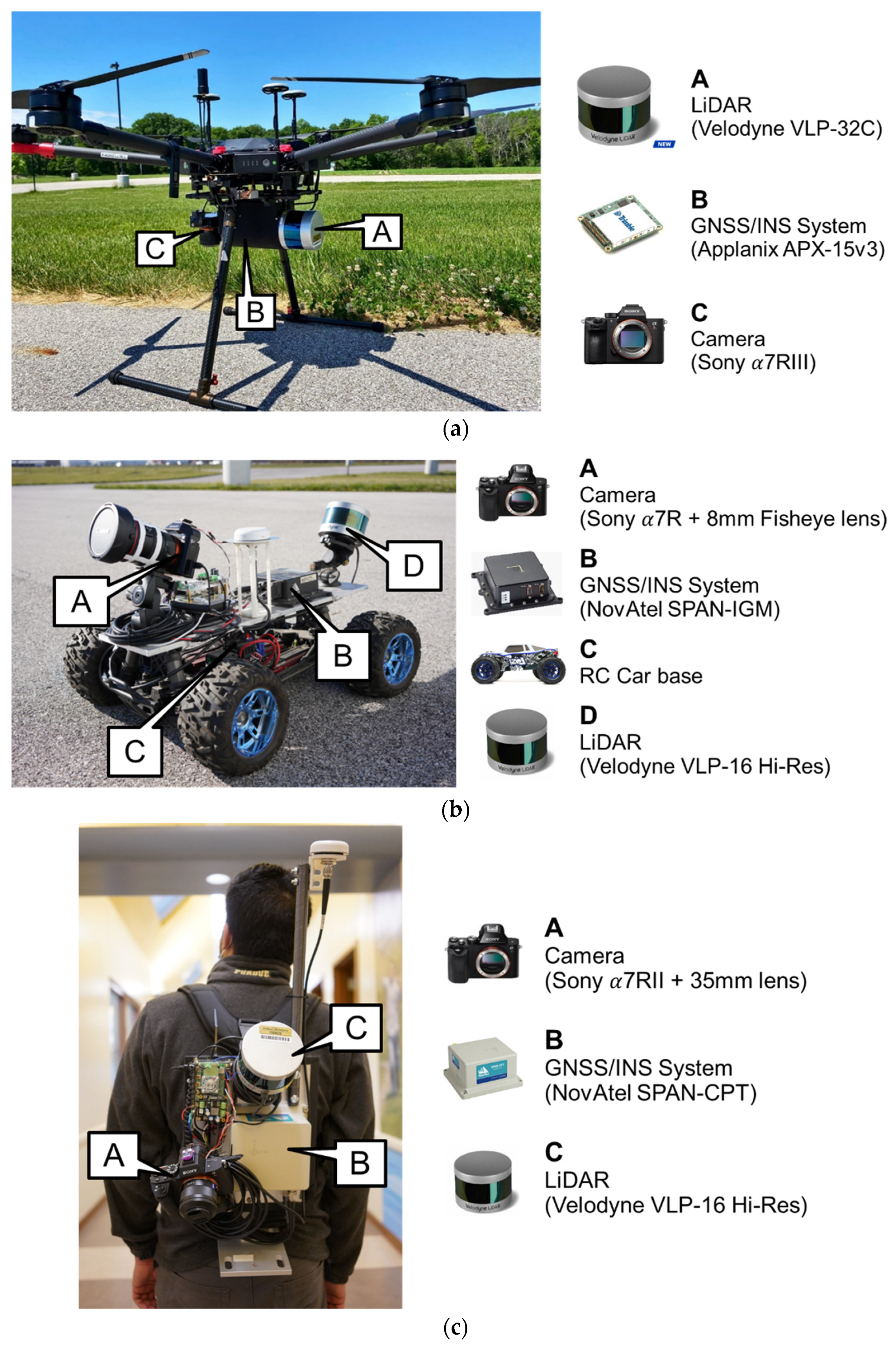
3.1. Specifications of Different MLMS Units

A total of six mobile mapping systems are used in this study: an unmanned aerial vehicle (UAV), an unmanned ground vehicle (UGV), a backpack-mounted portable system (hereafter called Backpack), the portable system mounted on a carrier vehicle (hereafter called Mobile-pack), a medium-grade wheel-based system: Purdue wheel-based mobile mapping system—high accuracy (PWMMS-HA), and a high-grade wheel-based system: Purdue wheel-based mobile mapping system—ultra-high accuracy (PWMMS-UHA). All the six MLMS units utilize direct georeferencing, i.e., the position and orientation information of the onboard sensors are directly obtained by an integrated global navigation satellite systems/inertial navigation systems (GNSS/INS). Figure 1 shows the six MLMS units together with the onboard sensors.

Table 1. Specifications of the georeferencing and LiDAR sensors for each mobile LiDAR mapping system (MLMS) including the approximate total cost.

	UAV	UGV	Backpack/ Mobile-Pack	PWMMS-HA		PWMMS-UHA
GNSS/INS Sensors	Applanix APX15v3	NovAtel SPAN-IGM-S1	NovAtel SPAN-CPT	Applanix POS LV 220		NovAtel ProPak6; IMU-ISA-100C
Sensor Weight	0.06 kg	0.54 kg	2.28 kg	2.40 + 2.50 kg		1.79 + 5.00 kg
Positional Accuracy	2–5 cm	2–3 cm	1–2 cm	2–5 cm		1–2 cm
Attitude Accuracy (Roll/Pitch)	0.025°	0.006°	0.015°	0.015°		0.003°
Attitude Accuracy (Heading)	0.08°	0.02°	0.03°	0.025°		0.004°
LiDAR Sensors	Velodyne VLP-32C	Velodyne VLP-16 High-Res	Velodyne VLP-16 High-Res	Velodyne VLP-16 High-Res	Velodyne HDL-32E	Riegl VUX 1HA	Z+F Profiler 9012
Sensor Weight	0.925 kg	0.830 kg	0.830 kg	0.830 kg	1.0 kg	3.5 kg	13.5 kg
No. of Channels	32	16	16	16	32	1	1
Pulse repetition rate	600,000 point/s (single return)	~300,000 point/s (single return)	~300,000 point/s (single return)	~300,000 point/s (single return)	~695,000 point/s (single return)	Up to 1,000,000 point/s	Up to 1,000,000 point/s
Maximum Range	200 m	100 m	100 m	100 m	100 m	135 m	119 m
Range Accuracy	$\pm$3 cm	$\pm$3 cm	$\pm$3 cm	$\pm$3 cm	$\pm 2$ cm	$\pm$5 mm	$\pm$2 mm
MLMS Cost (USD)	~$60,000	~$37,000	~$36,000	~$190,000		~$320,000

lists the specifications of the georeferencing [45,46,47,48,49] and LiDAR units [50,51,52,53,54] for each MLMS including the approximate total cost of the equipment.

While the specifications of a LiDAR sensor are critical in determining the resulting point cloud density, sensor orientation and sensor-to-object distance play an important role in defining the most relevant field of view which provides the highest number of beam returns from a given region of interest (ROI). The UAV system is built in a way that the rotation axis of the LiDAR unit is approximately parallel to the flying direction. The UGV LiDAR unit, owing to its tilt and proximity to the ground, produces a highly dense point cloud, but the useful scan area is limited to a very small field of view. The backpack system has a similar orientation of its LiDAR unit as that of the UGV; however, the unit, being positioned at least a meter above the ground, enables scanning a large surface area for the same angle subtended at the LiDAR unit as that of the UGV. The LiDAR sensors onboard the PWMMS-HA have only a slight tilt towards the ground, meaning each sensor covers a very large ground surface area. One would expect the resulting point cloud from PWMMS-HA to be sparse. On the contrary, as an advantage of having multiple sensors on the platform, any sparsity of points due to the large ground scan area is compensated by the additional LiDAR units through accurate system calibration. In case of the PWMMS-UHA, which is outfitted with two high-precision profiler LiDAR units, the sensors have similar tilts as the UGV. Additionally, the high pulse repetition rates of the LiDAR units allow for obtaining a high-density point cloud of the ground surface. Thus, selecting a suitable MLMS with an optimal sensor configuration is the key to deriving high density point cloud for a detailed mapping of roadside ditches from the acquired LiDAR data.

3.2. System Calibration of Different MLMS Units

The raw data collected by various MLMS units includes LiDAR range and intensity measurements, camera images, and georeferencing information from the GNSS/INS unit. In order to reconstruct accurately georeferenced and well-registered point cloud as well as to integrate the information from cameras, a system calibration procedure that estimates the relative position and orientation (hereafter, denoted as mounting parameters) between the LiDAR and imaging sensors and the GNSS/INS unit is required. The mounting parameters in this study are accurately estimated using the in-situ calibration procedure proposed by Ravi et al. [55]. This procedure estimates the mounting parameters by minimizing discrepancies among conjugate points, linear features, and/or planar features obtained from different LiDAR units and cameras in different drive-runs/flight lines.

Table 2. The range of standard deviation of the estimated system mounting parameters for all the LiDAR/camera units onboard each MLMS.

		UAV	UGV	Backpack/Mobile-Pack	PWMMS-HA	PWMMS-UHA
LiDAR units	Lever Arm	±1.2–1.5 cm	±1.0–1.3 cm	±0.5–0.8 cm	±0.8–1.8 cm	±0.5–0.6 cm
	Boresight	±0.02–0.04°	±0.02–0.08°	±0.02–0.03°	±0.02–0.05°	±0.01–0.02°
Camera units	Lever Arm	±2.7–5.4 cm	±3.7–6.5 cm	±3.0–4.9 cm	±3.8–6.6 cm	±3.1–6.0 cm
	Boresight	±0.03–0.04°	±0.12–0.14°	±0.08–0.12°	±0.07–0.14°	±0.06–0.11°

shows the range of standard deviation of estimated mounting parameters for all LiDAR units/cameras onboard each MLMS from the system calibration. The lever arm component along the Z direction ($\mathsf{\Delta }\mathrm{Z}$) was determined by incorporating real-time kinematic global navigation satellite systems (RTK-GNSS) survey measurements in the calibration model as vertical control. The accuracy of the final ground coordinates for each MLMS at a specified sensor-to-object distance was evaluated using the LiDAR Error Propagation calculator developed by Habib et al. [56]. The results, as shown in

Table 3. Expected accuracy of the ground coordinates evaluated using the LiDAR Error Propagation calculator [56].

	UAV	UGV	Backpack/ Mobile-Pack	PWMMS-HA	PWMMS-UHA
Suggested sensor-to-object distance	50 m	5 m	5 m	30 m	30 m
Corresponding accuracy	±5–6 cm	±2–4 cm	±2–3 cm	±2–3 cm	±1–2 cm
Accuracy at 50 m	±5–6 cm	±3–7 cm	±3–4 cm	±3–6 cm	±2–3 cm

, indicate that an accuracy of under 5–6 cm is achievable from all systems.

Once the mounting parameters are estimated accurately, the LiDAR point clouds and images captured by individual sensors onboard the systems can be directly georeferenced to a common reference frame. More specifically, using the estimated mounting parameters, together with the GNSS/INS trajectory, one can reconstruct a georeferenced LiDAR point cloud, and obtain the position and orientation of the camera in a global mapping frame whenever an image is captured. This capability allows for a forward and backward projection between the reconstructed point cloud and camera imagery.

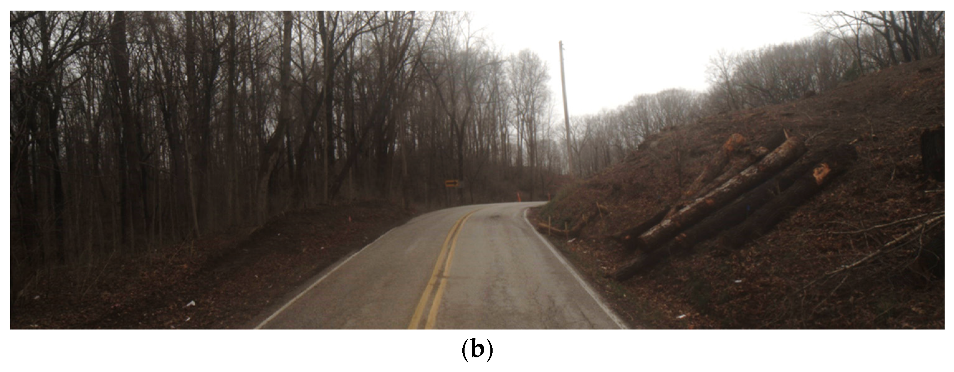
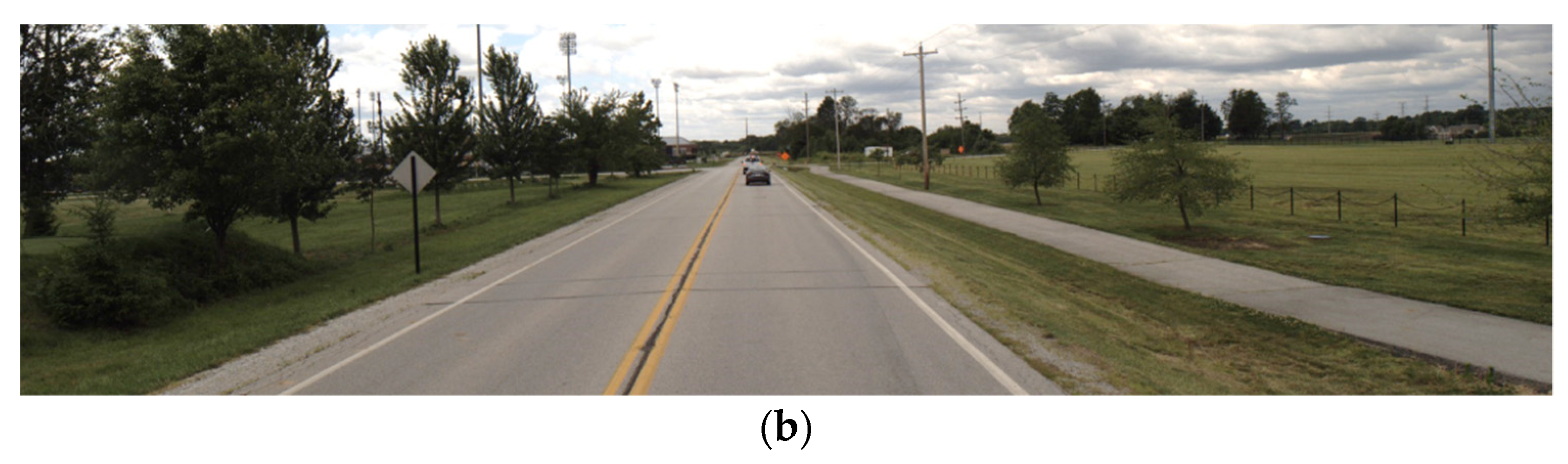
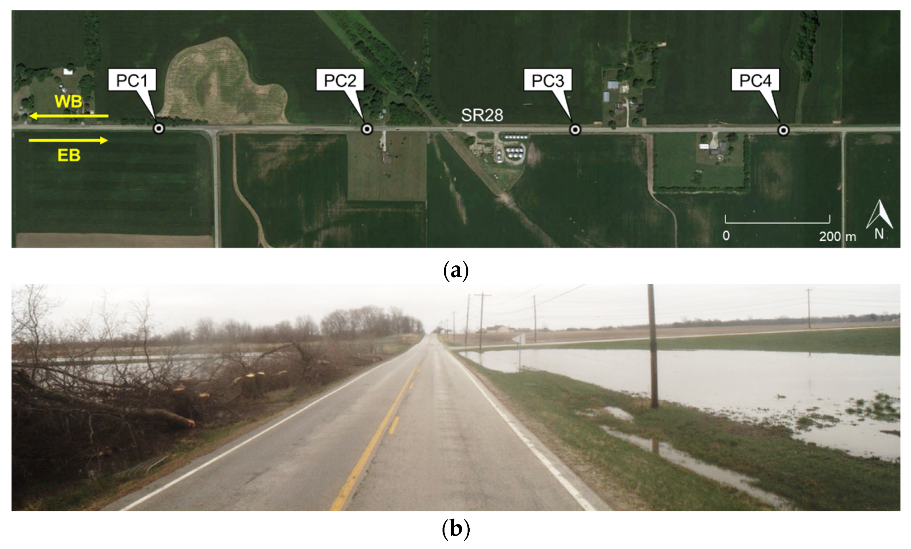
3.3. Dataset Description

A total of ten datasets were collected by different mobile LiDAR mapping systems over three study sites.

Table 4. Specifications of acquired datasets by the different MLMS units for this study. WB: westbound; EB: eastbound.

ID	Location	Data Collection Date	System	Number of Tracks	Average Speed (mph)	Data Acquisition Time (min)	Length (mile)
A-1	CR500N	13 March 2021	UAV	4	8	12	0.4
A-2		26 March 2021	PWMMS-HA	2	29	4	0.5
A-3		26 March 2021	Mobile-pack	2	20	4	0.5
B-1	McCormick Rd. and Cherry Ln.	22 December 2020	PWMMS-HA	2	20	10	1.6
B-2		22 December 2020	PWMMS-UHA	2	20	10	1.6
B-3		22 December 2020	UGV	4	4	30	0.5
B-4		22 December 2020	Backpack	4	3	32	0.5
B-5		26 March 2021	Mobile-pack	2	26	4	1.1
C-1	SR28	26 March 2021	PWMMS-HA	2	47	37	13.2
C-2		26 March 2021	Mobile-pack	2	50 (WB)/30 (EB)	35	13.2

lists the drive-run/flight configuration of each dataset. The performance of ground MLMS units for mapping roadside ditches is assessed against one of the well-studied aerial data acquisition methods, UAV, using datasets A-1, A-2, and A-3. Datasets B-1 to B-5 are used to evaluate the comparative performance between different ground MLMS units and identify the most practical ditch mapping solution. Finally, the proposed ditch line characterization strategies are tested using datasets C-1 and C-2.

Datasets A-1, A-2, and A-3 were collected over a county road, CR500N, in Indiana, USA. An aerial photo of the study site is presented in Figure 2a, and an image capturing location PA1 taken by the front left camera on the PWMMS-HA is shown in Figure 2b. This study site is located at a densely vegetated hill, as can be seen from the aerial photo. The average slope along the road is 6% (approximately 20 m elevation change over a planimetric distance of 350 m). The roadside ditches are present on both sides of the road and covered by short vegetation. At the time of this data acquisition, the indicated study site was being reworked to change the S-curve of the road to a simple curve with the goal of improving traffic safety. Cut trees for the road rework can be seen on the right side in Figure 2b. The PWMMS-HA and Mobile-pack drove along the road in both directions. The UAV was flown in four tracks over the study site with a flying height of 50 m above ground and a lateral distance of 14 m between neighboring flight lines.

Datasets B-1 to B-5 were collected at the intersection of McCormick Road and Cherry Lane adjacent to Purdue University’s campus in West Lafayette, Indiana, USA. The roadside ditches are present on both sides of the road and are covered by short vegetation. The width of these ditches ranges from 2 to 10 m, and their depth ranges from 0.2 to 1 m. Figure 3 shows an aerial photo of the study site and an image capturing location PB3 taken by the front left camera on the PWMMS-HA. To evaluate the absolute accuracy of the LiDAR-based mapping of the ditches, an RTK-GNSS survey was carried out at four cross-section locations—PB1, PB2, PB3, and PB4 in Figure 3a. For each profile, the team surveyed few points on the road and 20 to 25 points across the ditch. The team also took few measurements on the sidewalk that was adjacent to the road in profiles PB3 and PB4. The PWMMS-HA, PWMMS-UHA, UGV, and Backpack data were acquired on the same date when the RTK-GNSS survey was conducted. The PWMMS-HA and PWMMS-UHA covered all routes in both directions, so both datasets have two tracks. The UGV and Backpack acquired data along the ditches on both sides of the road in forward and backward directions, resulting in four tracks over the surveyed area. The Mobile-pack data was acquired at a later date (approximately three months from the RTK-GNSS and other MLMS surveys, refer to Table 4). The system drove along Cherry Lane and the south part of McCormick Road in both directions. Location PB1 was not covered in this survey.

Datasets C-1 and C-2 were collected over a state road, SR28, in Indiana, USA, with a total length of approximately 13 miles. The roadside ditches are present on both sides of the road and are covered by short vegetation and shrubs. A one-mile-long segment was selected as the ROI. Figure 4a shows an aerial photo of the ROI where PC1, PC2, PC3, and PC4 are four cross-section locations that are used in the ditch line characterization analysis (as will be discussed later in Section 5.3). Figure 4b is an image capturing location PC1 taken by the front left camera on the PWMMS-HA. As can be seen in the image, some parts of the ditches and adjacent agricultural fields were flooded. Some cut-down trees for an upcoming road maintenance project could also be seen. Both PWMMS-HA and Mobile-pack drove westbound and eastbound on SR28, and therefore both datasets have two tracks. The PWMMS-HA drove at an average speed of 47 mph in both directions. The Mobile-pack drove at a higher speed (50 mph) westbound and at a lower speed (30 mph) eastbound. This drive-run configuration was designed to investigate the impact of driving speed on point density as well as to evaluate the system’s ability to map roadside ditches.

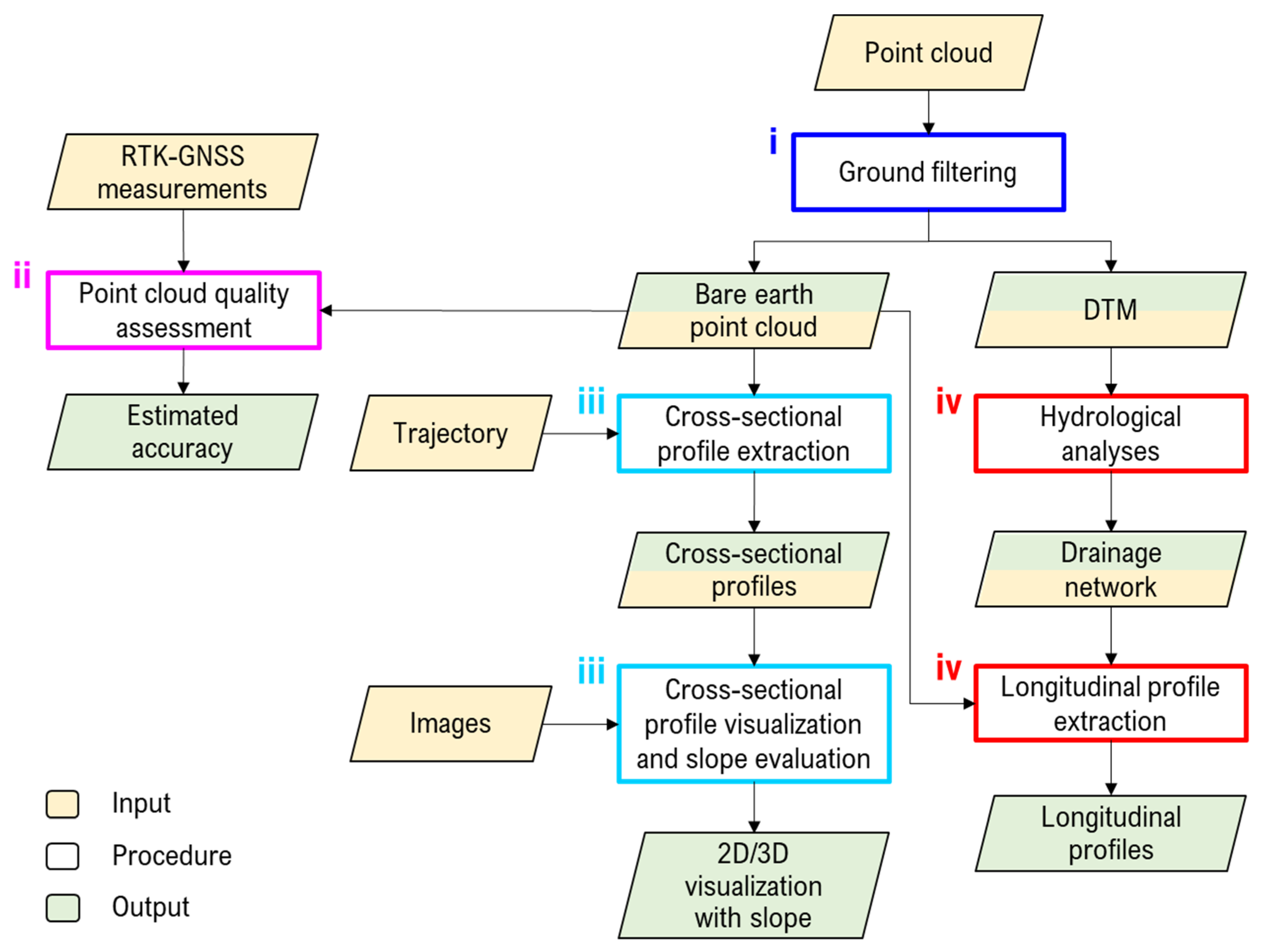
4. Methodology for Ditch Mapping and Characterization

The proposed framework for roadside ditch mapping is illustrated in Figure 5. The main steps include (i) ground filtering; (ii) point cloud quality assessment; (iii) cross-sectional profile extraction, visualization, and slope evaluation; and (iv) drainage network and longitudinal profile extraction.

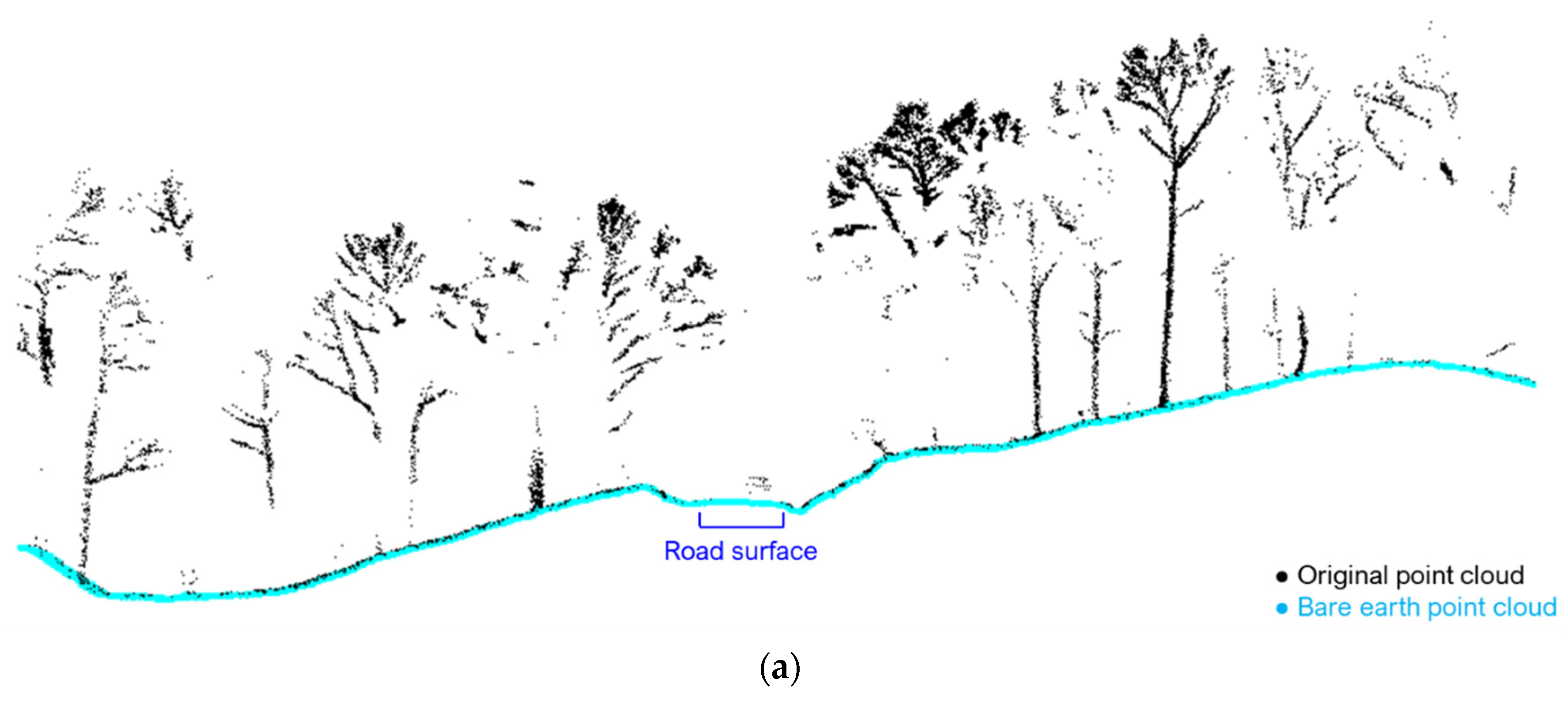
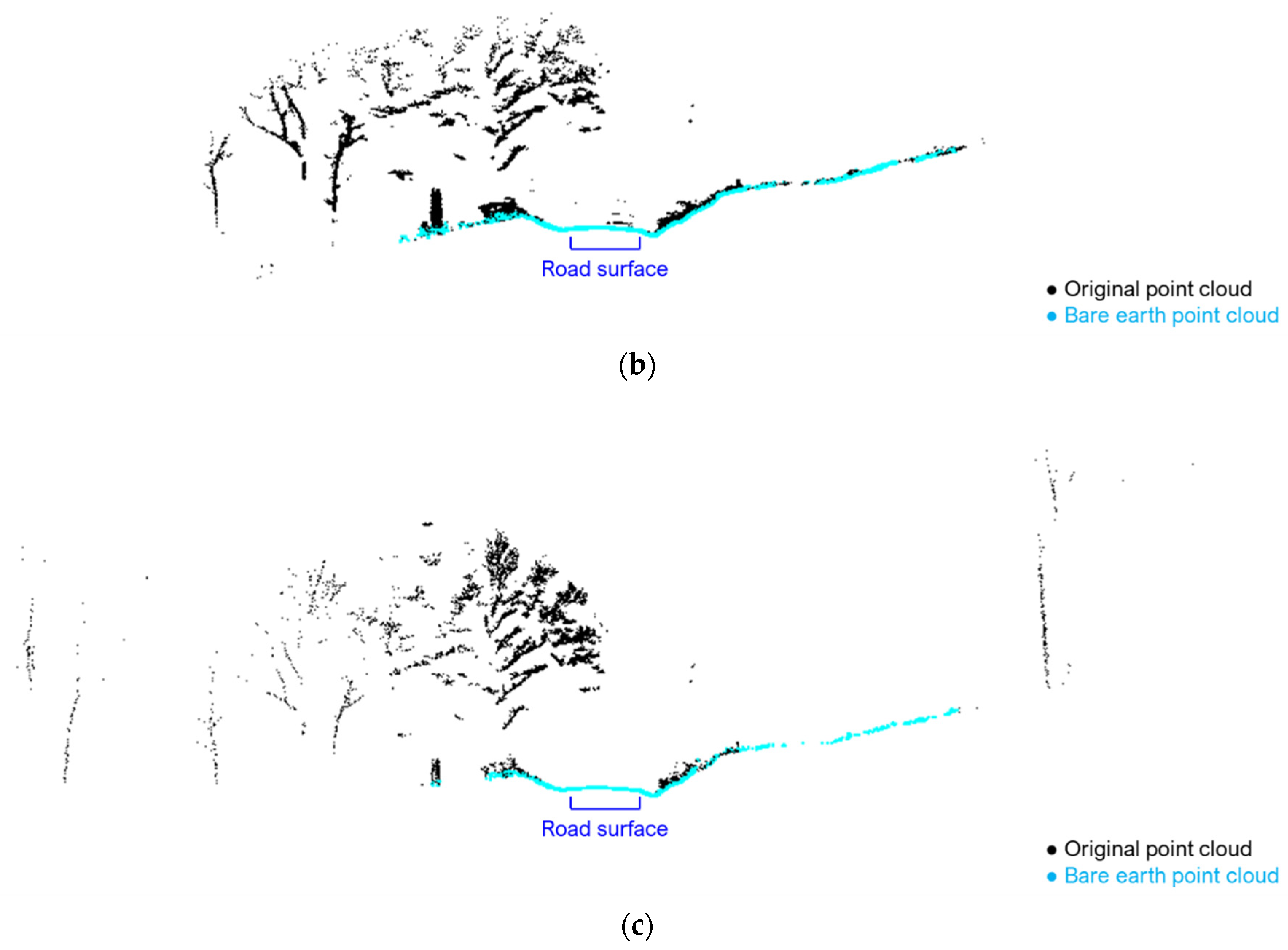
4.1. Ground Filtering

The cloth simulation algorithm proposed by Zhang et al. [57] is modified to handle the large variation in point density of mobile LiDAR data. The original cloth simulation approach can be summarized in four steps: (i) turn the point cloud upside down, (ii) define a cloth (consisting of particles and their interconnections) with some rigidness and place it above the point cloud, (iii) let the cloth drop under the influence of gravity to designate the final shape of the cloth as the DTM, and (iv) use the DTM to filter the ground from above-ground points. Here, the rigidness of the cloth is constant, and its value is selected based on the properties of the terrain. The modified approach redefines the rigidness of each particle on the cloth based on the point density of an initial bare earth point cloud. The approach is implemented in C++, and it consists of three steps: (i) using the original approach to extract the bare earth point cloud, (ii) redefining the rigidness of the cloth based on the point density of the bare earth point cloud, and (iii) applying the cloth simulation again to obtain a refined bare earth point cloud and the final DTM.

An example of a DTM generated based on the original and modified approaches is shown in Figure 6. A ground truth DTM was generated using the PWMMS-HA point cloud, which has full coverage over the ROI (Figure 6a). The original and modified approaches were then applied to generate DTM from the UGV point cloud (Figure 6b), where large variation in point density can be observed. The side view of a cross-sectional profile is illustrated in Figure 6c to highlight the obvious differences in the DTM due to sparse points. The original approach leads to artifacts in low point density areas, as the cloth keeps dropping without being stopped by the ground. By manipulating the rigidness of the cloth depending on the point density within the neighborhood, the modified approach is able to generate a reasonable representation of the terrain, even if there are gaps in the point cloud.

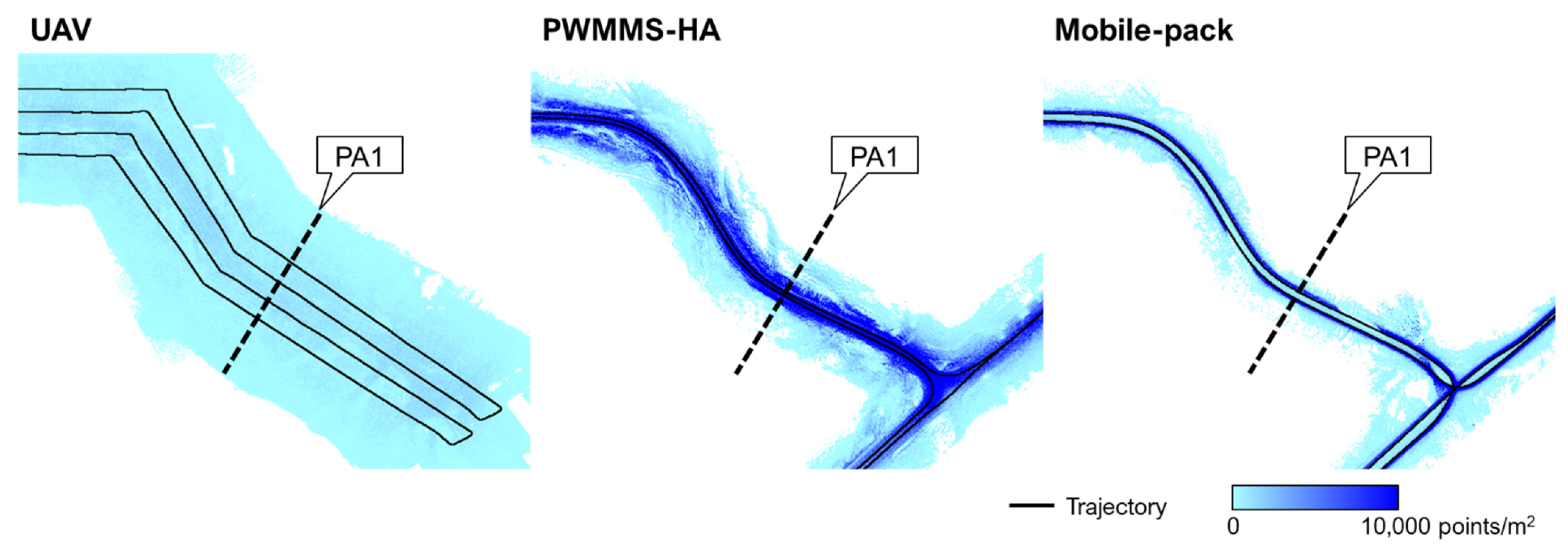
4.2. Point Cloud Quality Assessment

Quality assessment involves evaluating the (i) relative accuracy: alignment between point clouds from different MLMS units, and (ii) absolute accuracy: agreement between the point cloud and independently measured ground control points.

In this study, two approaches are adopted to evaluate the relative accuracy: the feature-based quality assessment [58] and the multiscale model-to-model cloud comparison (M3C2) [59]. In Lin and Habib [58], the assessment of relative accuracy between two point clouds quantifies the degree of consistency among conjugate points/features. Planar features—terrain patches—extracted from the bare earth point cloud are used to provide discrepancy information. The net discrepancy along the X, Y, and Z directions between two point clouds is estimated using a least squares adjustment (LSA) with modified weight matrix [60,61]. One should note that the reliability of these estimates depends on the variation in the orientation/slope/aspect within the ROI. For transportation corridors, the terrain patches are mostly flat or have a mild slope and thus provide discrepancy information mainly along the vertical direction. Therefore, only the vertical discrepancy estimation is reported. The M3C2 distance is a signed normal distance between two point clouds along the local surface direction [59]. It represents the 3D variations in surface orientation.

The absolute accuracy is assessed against manually collected RTK-GNSS measurements (hereafter, RTK points). To investigate the LiDAR mapping accuracy over different surfaces, we manually classify the LiDAR/RTK points into two classes: solid surface (including road and sidewalk) and vegetated area. The elevation difference between each RTK point and its closest LiDAR point is calculated, and the root–mean–square error (RMSE) and interquartile range are reported for each class.

4.3. Cross-Sectional Profile Extraction, Visualization, and Slope Evaluation

A cross-sectional profile with a given length and width can be extracted from the point cloud, bare earth point cloud, and/or DTM at any location. The orientation of the profile should be perpendicular to the direction of the road, which can be derived using the vehicle trajectory information. Once the profile is extracted, the slope along the profile is evaluated using the bare earth points; a sample result is shown in Figure 7. The profile and slope information extracted from LiDAR data can then be compared to the design/standard values [62] to detect problems such as improper grade. Furthermore, using the trajectory information, it is possible to crop and analyze a series of cross-sectional profiles automatically based on a user-defined interval.

The key strength of mobile mapping systems lies in the integration of information acquired from different sensors onboard the system. Since all the sensors’ data are georeferenced to a common reference frame, multi-sensor/multi-date datasets can be effectively fused. That is, the images capturing each profile can be identified, and the profile can be back-projected onto the images. Consequently, the ditches can be visualized in both 3D point clouds and 2D images, even though they are mainly detected and mapped in 3D space. The image-based visualization is useful for effective mitigation of detected problems during ditch mapping (e.g., deviation from the design profile of the ditch, improper grade, and/or debris within the ditch).

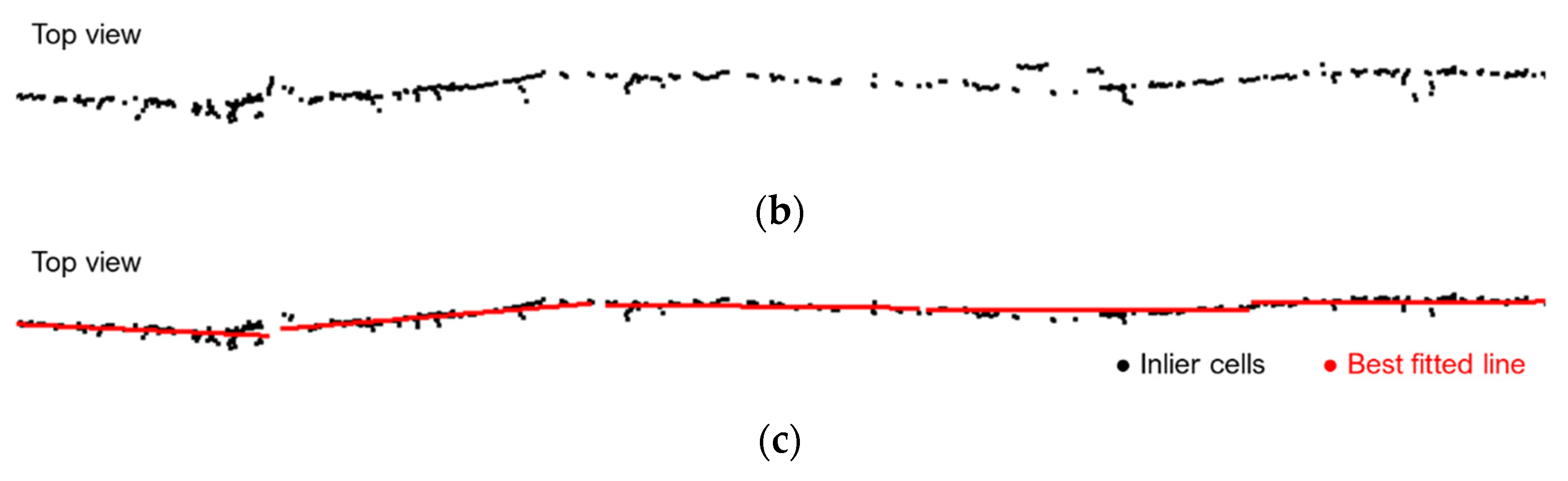
4.4. Drainage Network and Longitudinal Profile Extraction

Conducting a drainage network analysis is critical because it signifies the location of valley points along the ditches and also identifies potential drainage issues. The drainage network through which water travels can be identified by analyzing the movement of surface water, that is, calculating the flow direction and flow accumulation for each DTM cell [63]. When enough water flows through a cell, the location is considered to have a stream passing through it. Therefore, the drainage network can be extracted by applying a user-defined threshold on the flow accumulation map.

A longitudinal profile is the one along the “valley” of a ditch; that is, it aligns with the major stream in the drainage network. Figure 8a shows an example of the drainage network extracted from MLMS data, from which some tributaries and discontinuities along the major streams can be observed. To identify the location of the longitudinal profile, we need to remove tributaries and connect major streams. Since our focus is the ditches adjacent to a transportation corridor, the drainage network is expected to be a long, linear feature. Line fitting is performed to estimate the line parameters, which, in turn, are used to find the direction of the major stream. The drainage network is then rotated so that the direction of the major stream is along the X-direction. The tributaries are removed based on the assumption that within a small range of the X-coordinate of the rotated drainage network, the elevation of the major stream is lower than the elevation of the tributaries. A sample result is shown in Figure 8b. Next, we divide the streamlines into segments and apply line fitting and outlier removal using a random sample consensus (RANSAC) strategy [64], depicted in Figure 8c, assuming that the ditch line is approximately a straight line within each segment. The longitudinal profile is extracted based on the location of the inlier streamlines and best-fitted lines. Figure 9 illustrates a sample longitudinal profile together with the detected lane marking that signifies the elevation of the road surface.

5. Experimental Results

In this section, we present three experimental results. The first experiment compares the ground systems to UAV in terms of their ability of mapping roadside ditches. The second experiment evaluates the comparative performance of different grades of MLMS and identifies the most feasible technique for ditch mapping. The third experiment tests the proposed ditch line characterization approach using a one-mile segment along a state road.

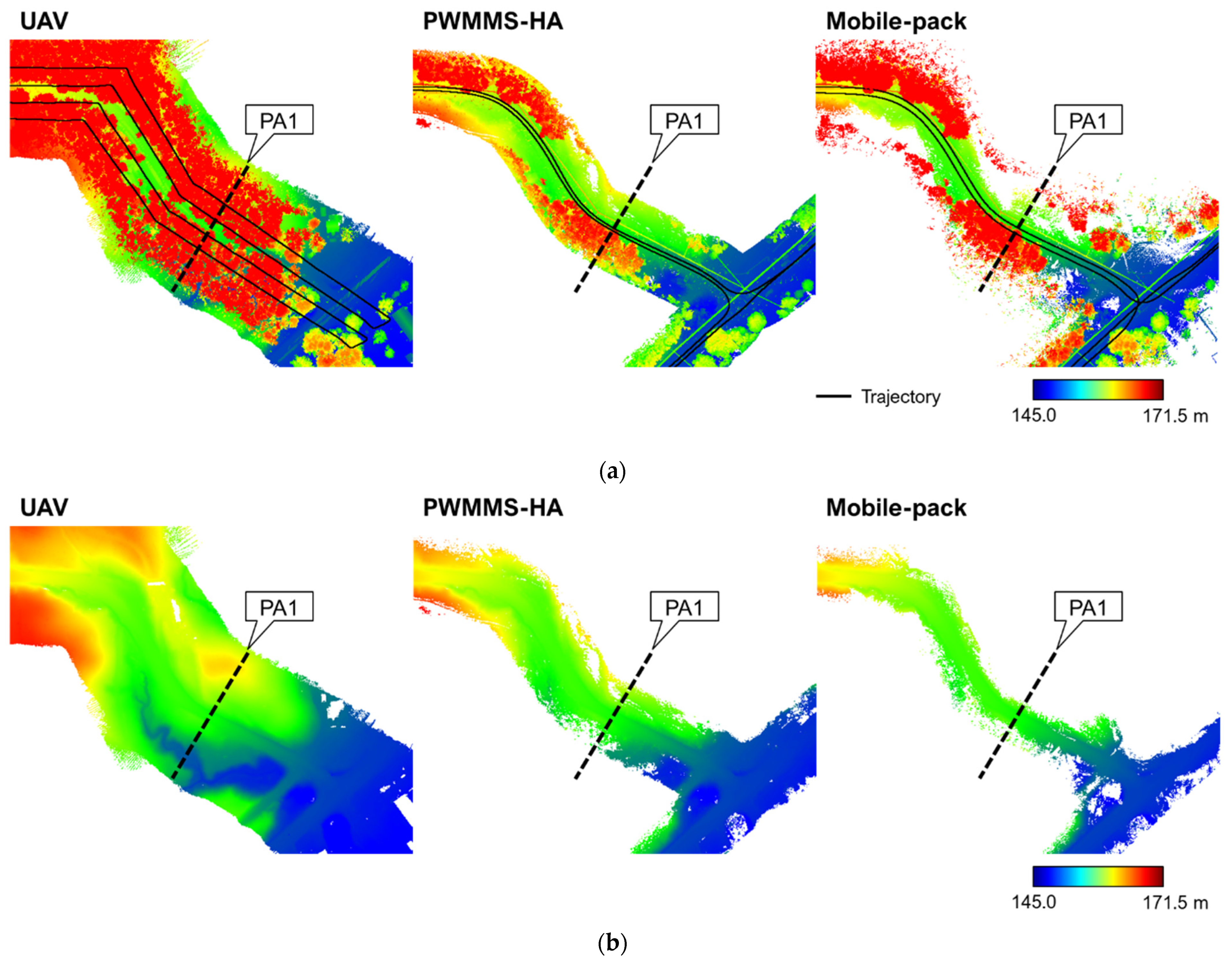
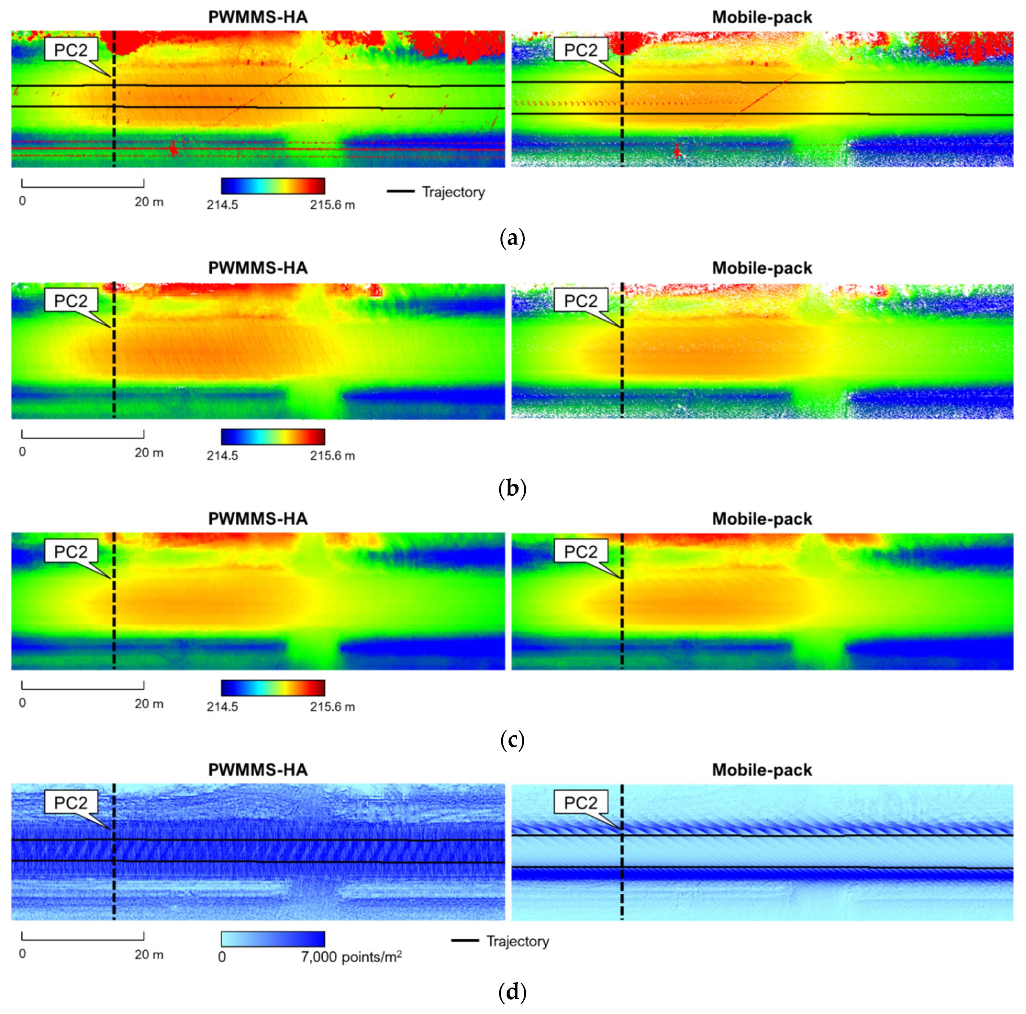
5.1. Comparison between Ground and UAV Systems for Mapping Roadside Ditches

In this section, the capability of ground MLMS for monitoring roadside ditches is assessed against a UAV-based MLMS. Datasets A-1 (captured by the UAV), A-2 (captured by the PWMMS-HA), and A-3 (captured by the Mobile-pack) were used for this analysis. The ground MLMS mapping products were compared to those from the UAV in terms of the spatial coverage, point density, and relative vertical accuracy between point clouds.

The point cloud and bare earth point cloud were first generated from each dataset. Figure 10a shows the point clouds from different MLMS units together with the trajectory. While the ground MLMS units can only drive on road, and therefore the point cloud coverage is limited to areas adjacent to the road, theoretically, there is no such limitation on the flight movement for the UAV. For the datasets used in the current analysis, the UAV was able to maneuver over a large area and obtain a wide spatial coverage. The bare earth point clouds were extracted using the modified cloth simulation approach, and the results are depicted in Figure 10b. A cross-sectional profile at location PA1 was extracted from the original and bare earth point clouds. The profile side view, as shown in Figure 11, demonstrates that the LiDAR points were able to penetrate the vegetation and capture the terrain. Compared to the UAV, the ground systems are more prone to occlusions caused by terrain features. Having said that, all three systems show complete coverage over the road surface and ditches, which are the focus of this study.

The point density map for each dataset was derived based on the bare earth point cloud since the latter is the one used for ditch line characterization. Figure 12 shows the point density maps along with the trajectory for the UAV, PWMMS-HA, and Mobile-pack. The statistics of point density, including the 25th percentile, median, and 75th percentile in the surveyed area, are reported in

Table 5. Statistics of the point density in the surveyed area.

Dataset	Point Density (Points/m2)
	25th Percentile	Median	75th Percentile
A-1 (UAV)	200	500	1000
A-2 (PWMMS-HA)	500	1800	6100
A-3 (Mobile-pack)	400	1200	3800

. The ground systems produced much higher point density as compared to the UAV due to the short sensor-to-object distance. PWMMS-HA had the highest point density since its point cloud came from four LiDAR units. Looking into the spatial pattern in Figure 12, the point density from the ground systems is high near the trajectory, and it decreases drastically as the distance from the trajectory increases. This spatial pattern is mainly related to the varying sensor-to-object distance and occlusion caused by trees. For the UAV, in contrast, the sensor-to-object distance (i.e., flying height) was almost constant throughout the data collection, and thus the variation in point density across the surveyed area is much smaller.

The relative vertical discrepancies between point clouds from different systems were estimated using the terrain patches extracted from the bare earth point clouds. The size of the terrain patches was set to 0.5 × 0.5 m. The square root of the a posteriori variance factor ($\widehat{{\sigma }_0}$) and the estimated vertical discrepancy ($d_z$) between the point clouds from different MLMS units are reported in

Table 6. Estimated vertical discrepancy ($d_z$) and square root of a posteriori variance ($\widehat{{\sigma }_0}$) using A-1 (UAV), A-2 (PWMMS-HA), and A-3 (Mobile-pack) datasets.

Reference	Source	Number of Observations	$\widehat{{\mathit{\sigma }}_0}\left(\mathbf{m}\right)$	${\mathit{d}}_{\mathit{z}}\left(\mathbf{m}\right)$
				Parameter	Std. Dev.
UAV	PWMMS-HA	111,973	0.083	0.028	2.615 $\times {10}^{-4}$
UAV	Mobile-pack	55,742	0.064	−0.008	2.864 $\times {10}^{-4}$
PWMMS-HA	Mobile-pack	67,133	0.043	−0.029	1.671 $\times {10}^{-4}$

. The former reflects the noise level of the point clouds, and the latter signifies the overall net discrepancy between the point clouds in question. According to Table 6, the square root of the a posteriori variance factor suggests a noise level of ±4–8 cm. The discrepancy estimation shows that all datasets are in agreement within a ±3 cm range along the vertical direction. In addition, the discrepancies between point clouds are estimated using the M3C2 distance. The two parameters, normal scale and projection scale, were set to 0.5 m. The minimum point spacing between two core points was set to 0.5 m. The statistics of the M3C2 distance, including mean, standard deviation, RMSE, and median, are reported in

Table 7. Discrepancy estimation based on model-to-model cloud comparison (M3C2) distance using A-1 (UAV), A-2 (PWMMS-HA), and A-3 (Mobile-pack) datasets.

Reference	Source	Number of Observations	M3C2 Distance (m)
			Mean	Std. Dev.	RMSE	Median
UAV	PWMMS-HA	93,124	0.034	0.068	0.076	0.030
UAV	Mobile-pack	50,123	0.001	0.074	0.074	−0.004
PWMMS-HA	Mobile-pack	63,408	−0.028	0.062	0.068	−0.027

. The results are in good agreement with the discrepancy estimated using terrain patches.

The discussion above reveals that all the MLMS units can achieve similar mapping accuracy. The advantage of UAV is that it can maneuver over areas that are difficult to reach by ground vehicles. Nonetheless, field surveys with ground MLMS units are more efficient since the vehicles can travel at a higher speed and cover a longer extent. As long as the ROI is limited to areas adjacent to the road, all the MLMS data can have full coverage with a decent point density, which is adequate for monitoring roadside ditches.

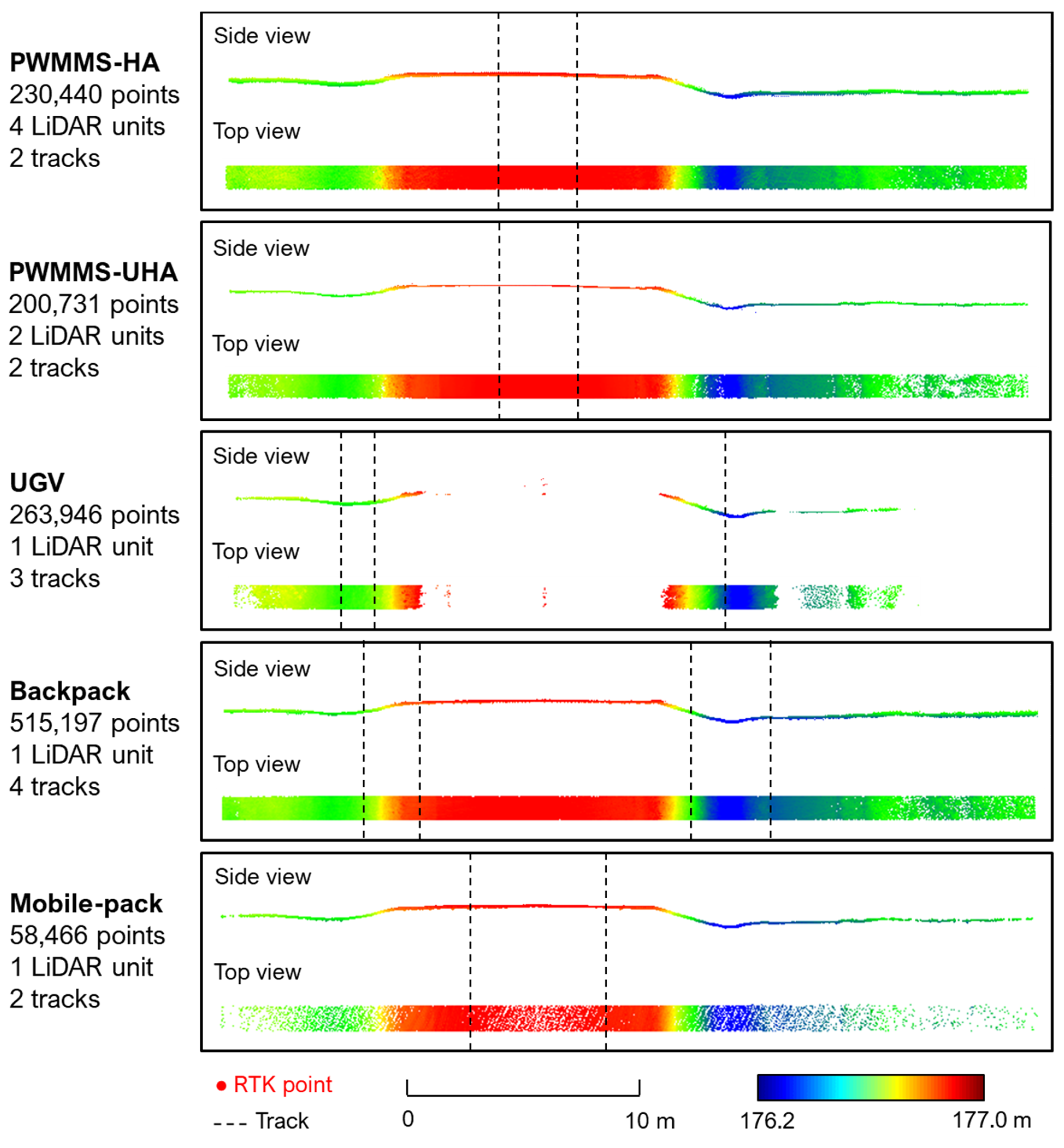
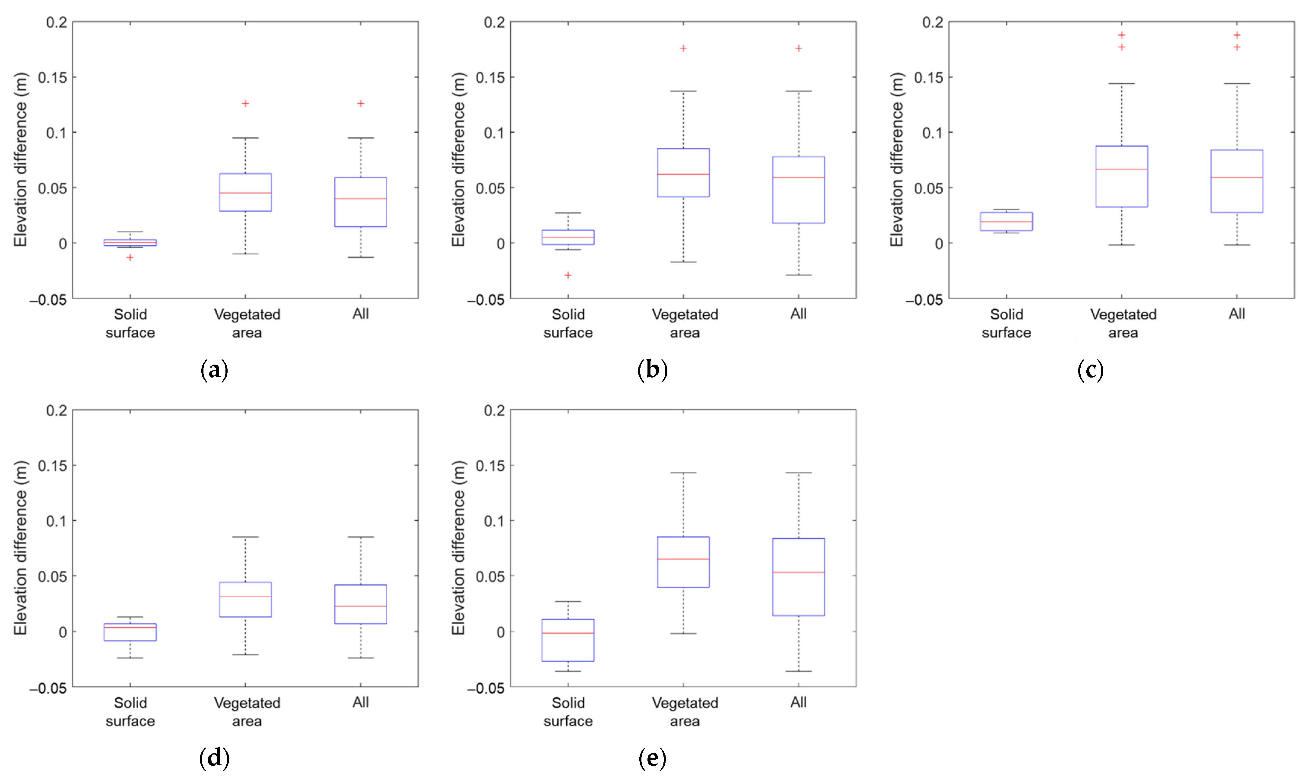
5.2. Comparative Performance of Different Ground MLMS Units

In this experiment, the ability of different ground MLMS units to map roadside ditches was evaluated. Datasets B-1 (captured by the PWMMS-HA), B-2 (captured by the PWMMS-UHA), B-3 (captured by the UGV), B-4 (captured by the Backpack), and B-5 (captured by the Mobile-pack) were used in this analysis. The comparative performance of different MLMS units was assessed in terms of spatial coverage, relative vertical accuracy, and absolute vertical accuracy.

Upon reconstructing the point cloud, the bare earth point cloud was extracted, and the DTM was generated using the modified cloth simulation approach for each dataset. Cross-sectional profiles at locations PB1, PB2, PB3, and PB4 were extracted from the point cloud, bare earth point cloud, and DTM with a width of 1 m. Figure 13 shows the cross-sectional profiles of the bare earth point clouds from different MLMS units at location PB3. The spatial coverage of point clouds from different systems was evaluated qualitatively. As can be observed in Figure 13, with sufficient number of tracks, each of the mobile mapping systems demonstrates a complete coverage of the ditch. The UGV point cloud, despite having full coverage over the ditches, has limited coverage of the road and areas that are away from the tracks. For the UGV, the location of tracks with respect to the ditch plays a crucial role. Since the UGV tends to be very close to the ground, it is prone to occlusions caused by surrounding vegetation and terrain. The Mobile-pack has the least number of points because it has only one LiDAR unit covering two tracks over the region of interest, and the vehicle to which the sensor assembly was mounted traveled at a speed similar to that of the PWMMS-HA and PWMMS-UHA. One thing to note is that the point density of Mobile-pack drops rapidly when moving away from the trajectory. This is attributed to the mounting orientation of its LiDAR sensor whose field of view was limited to focus on objects in short range (refer to Figure 1d and the discussion in Section 3.1). Figure 14 shows the side view of the cross-sectional profiles at locations PB1, PB2, PB3, and PB4 from the bare earth point cloud. Qualitatively, point clouds from different MLMS units are aligned well along the vertical direction. Over the ditch areas, the noise level of the point clouds is higher due to different degrees of penetration on vegetation.

The relative vertical accuracy between point clouds from different MLMS units was evaluated using planar features—terrain patches—extracted from the bare earth point clouds over the surveyed area. The size of the terrain patches was set to 0.5 × 0.5 m. The PWMMS-HA dataset was selected as a reference because it had the largest spatial coverage.

Table 8. Estimated vertical discrepancy ($d_z$) and square root of a posteriori variance ($\widehat{{\sigma }_0}$) using B-1 (PWMMS-HA), B-2 (PWMMS-UHA), B-3 (UGV), B-4 (Backpack), and B-5 (Mobile-pack) datasets.

Reference	Source	Number of Observations	$\widehat{{\mathit{\sigma }}_0}\left(\mathbf{m}\right)$	${\mathit{d}}_{\mathit{z}}\left(\mathbf{m}\right)$
				Parameter	Std. Dev.
PWMMS-HA	PWMMS-UHA	13,610	0.010	−0.013	8.711 $\times {10}^{-5}$
PWMMS-HA	UGV	4737	0.021	0.007	3.385 $\times {10}^{-4}$
PWMMS-HA	Backpack	12,480	0.012	−0.027	1.137 $\times {10}^{-4}$
PWMMS-HA	Mobile-pack	11,539	0.018	−0.019	1.750 $\times {10}^{-4}$

reports the square root of a posteriori variance factor ($\widehat{{\sigma }_0}$) and estimated vertical discrepancy ($d_z$) between the point clouds from different MLMS units. The square root of a posteriori variance factor suggests a noise level of ±1–2 cm. The discrepancy estimation using the M3C2 distance is reported in

Table 9. Discrepancy estimation based on M3C2 distance using A-1 (UAV), A-2 (PWMMS-HA), and A-3 (Mobile-pack) datasets.

Reference	Source	Number of Observations	M3C2 Distance (m)
			Mean	Std. Dev.	RMSE	Median
PWMMS-HA	PWMMS-UHA	11,279	−0.012	0.013	0.018	−0.013
PWMMS-HA	UGV	4018	0.012	0.028	0.031	0.008
PWMMS-HA	Backpack	10,272	−0.029	0.017	0.033	−0.029
PWMMS-HA	Mobile Backpack	10,261	−0.021	0.022	0.031	−0.022

. The normal scale, projection scale, and minimum point spacing between two core points was set to 0.5 m. Both the feature-based approach and M3C2 distance suggest that the point clouds from different MLMS units exhibit a good degree of agreement with an overall precision of ±1–3 cm.

The absolute accuracy of the point cloud from different MLMS units was assessed against the RTK-GNSS survey. Figure 15 shows the side view of the RTK points together with the bare earth point cloud and DTM from each MLMS at location PB3. Through visual inspection, one can see that the DTMs trace the terrain well and are in good agreement with the RTK points along the vertical direction. As mentioned in Section 4.2, the LiDAR/RTK points are classified into two classes: solid surface (including road and sidewalk) and vegetated area. The elevation difference between each RTK point and its closest LiDAR point is calculated, and the interquartile range is visualized, as shown in Figure 16. The variance of elevation differences is small for solid surfaces and large for vegetated areas. The vertical accuracy was found to be ±1 cm (PWMMS-HA), ±1 cm (PWMMS-UHA), ±2 cm (UGV), ±1 cm (Backpack), and ±2 cm (Mobile-pack) for solid surfaces. For areas with vegetation, the vertical accuracy was found to be ±5, ±7, ±7, ±4, and ±7 cm for PWMMS-HA, PWMMS-UHA, UGV, Backpack, and Mobile-pack, respectively. The PWMMS-HA and Backpack, despite with cm-level accuracy LiDAR units, had a slightly better performance, mainly attributed to better penetration of vegetated surfaces due to their higher point density and larger beam divergence angle of the Velodyne units.

In this section, the spatial coverage, relative vertical accuracy, and absolute vertical accuracy of point clouds from five ground MLMS units were evaluated. The results suggest that all the MLMS units can have a complete coverage of the roadside ditches with a sufficient number of tracks. UGV is less desirable because it is prone to occlusions. The ditch-mapping accuracy of different MLMS units was found to be similar. Systems with high-end LiDAR units are not necessarily better for mapping roadside ditches. In terms of field survey, UGV and Backpack are not practical for mapping long extents of transportation corridors. Consequently, the PWMMS-HA and Mobile-pack are practical solutions for mapping roadside drainage ditches.

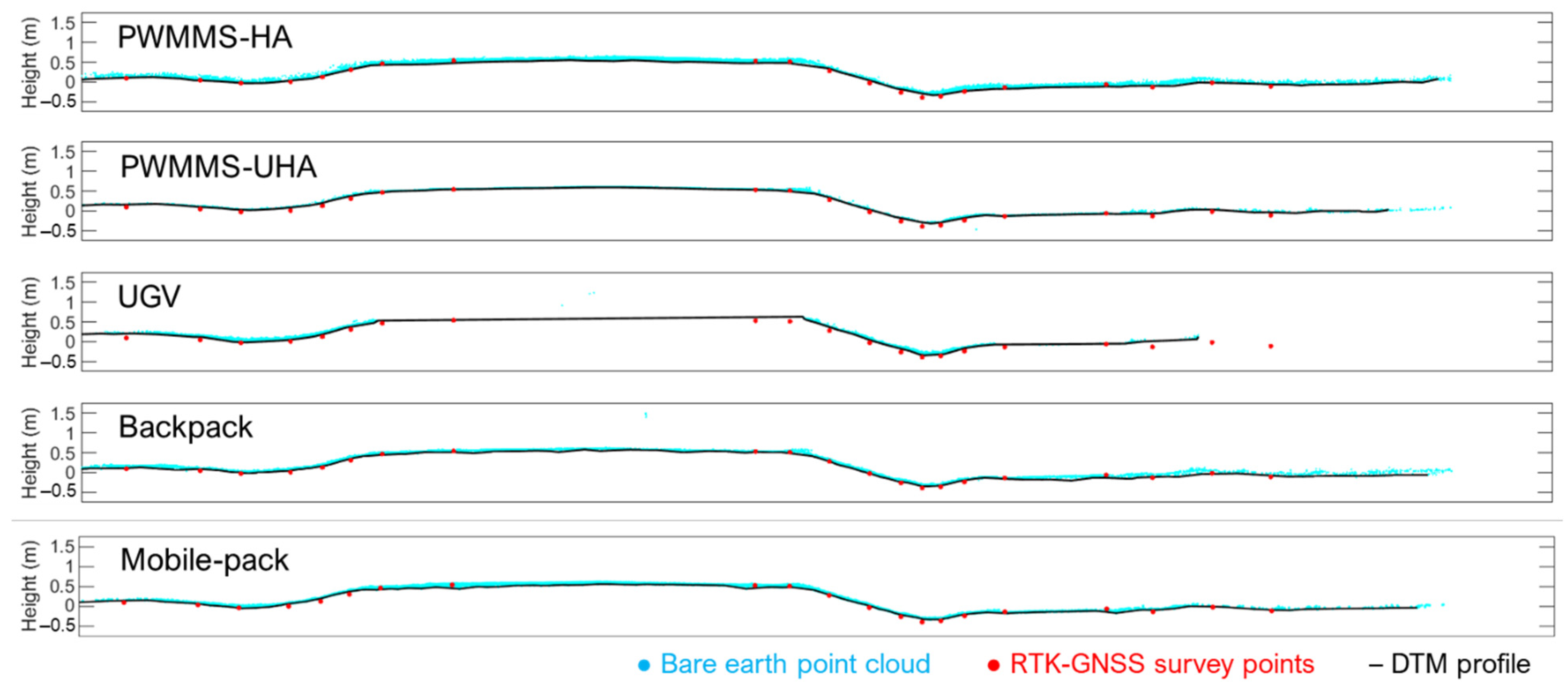
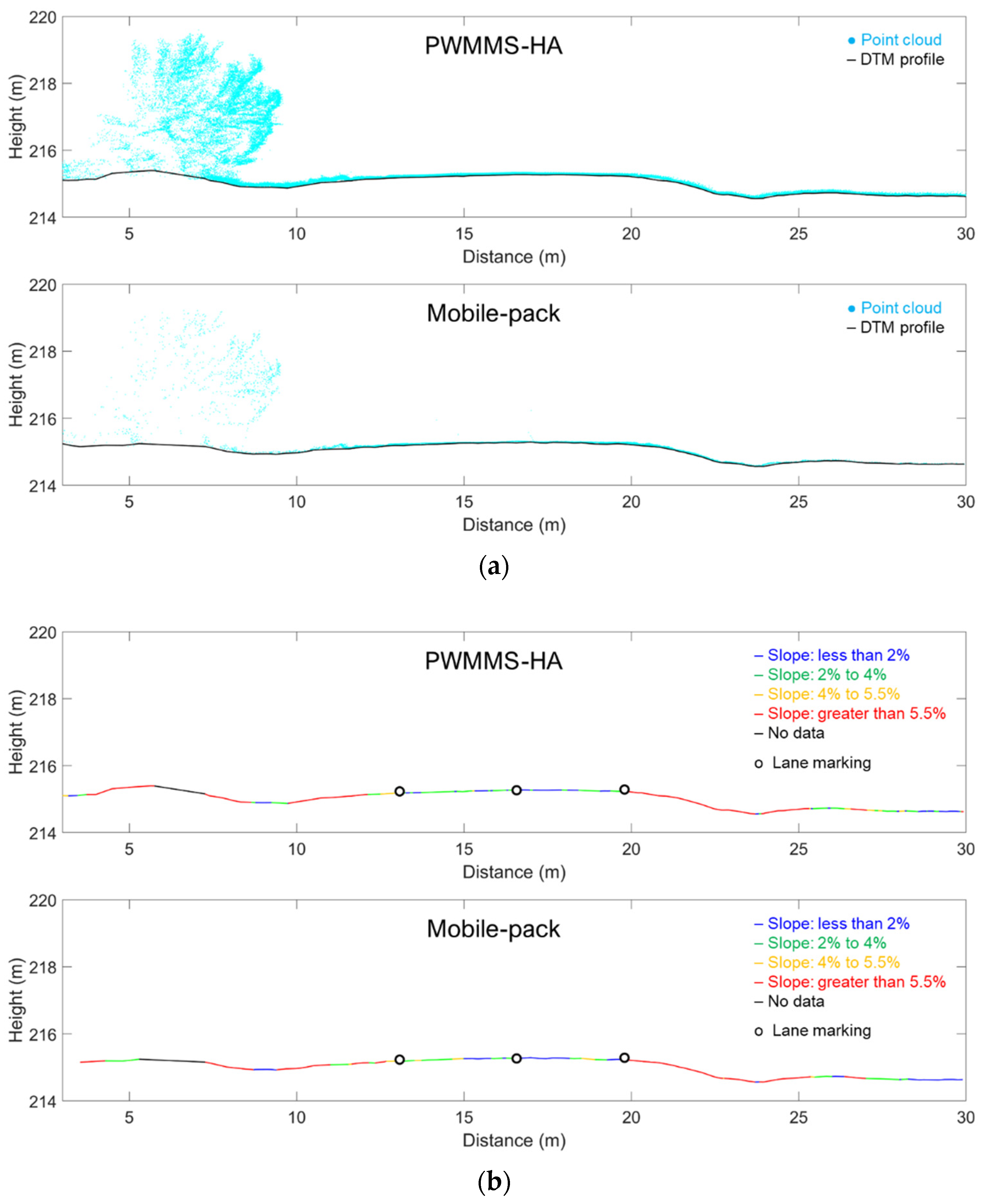
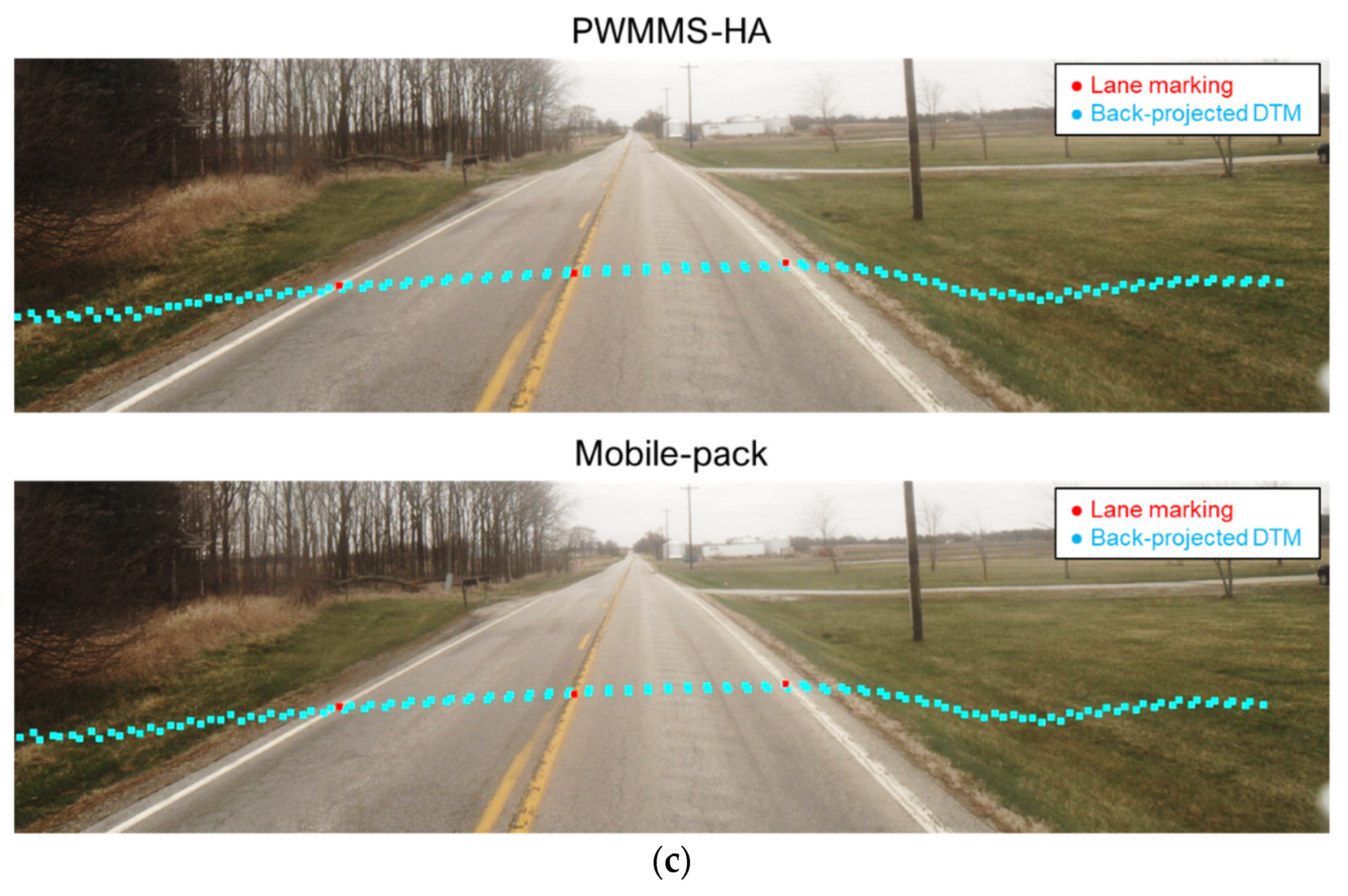
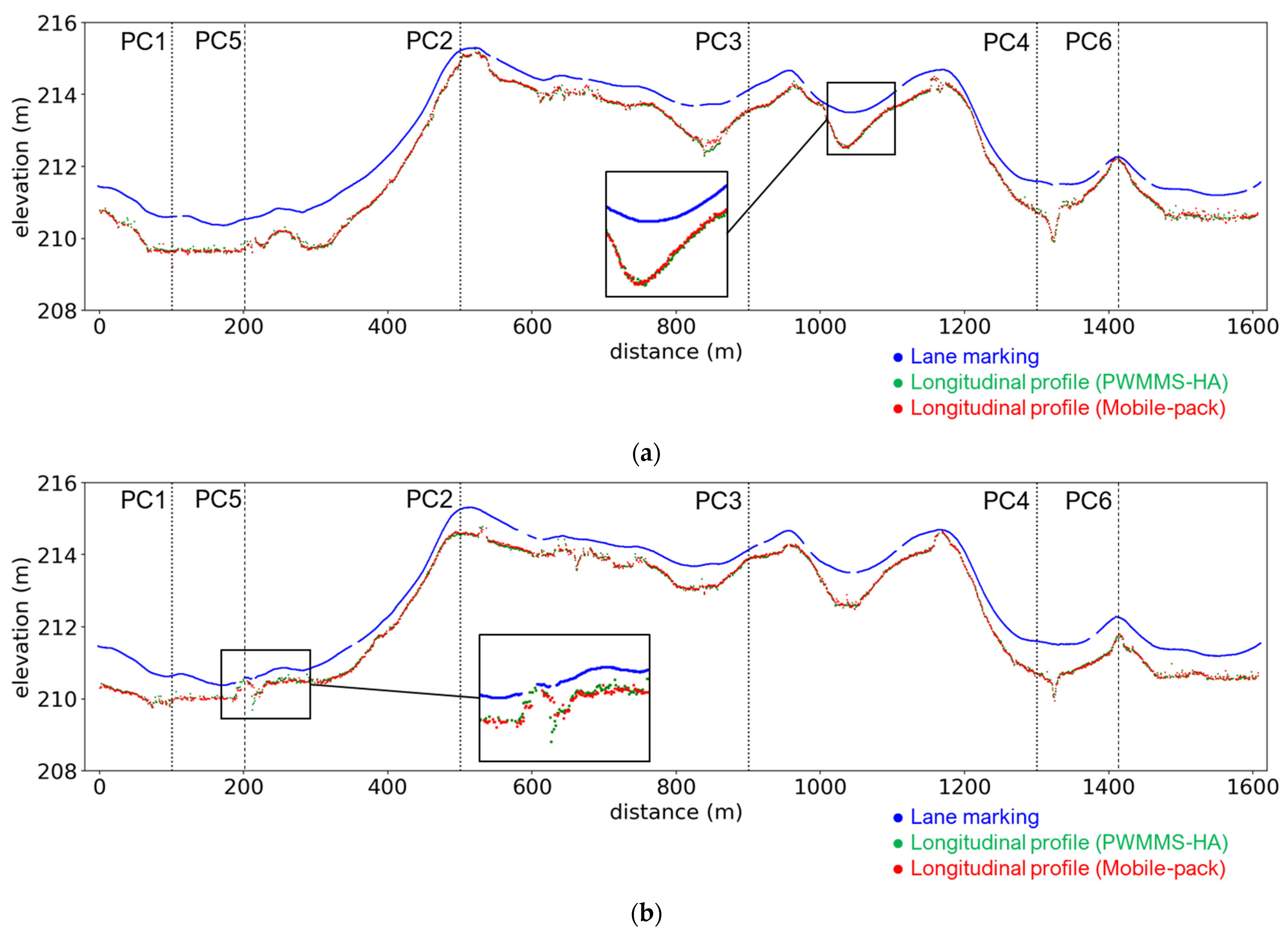
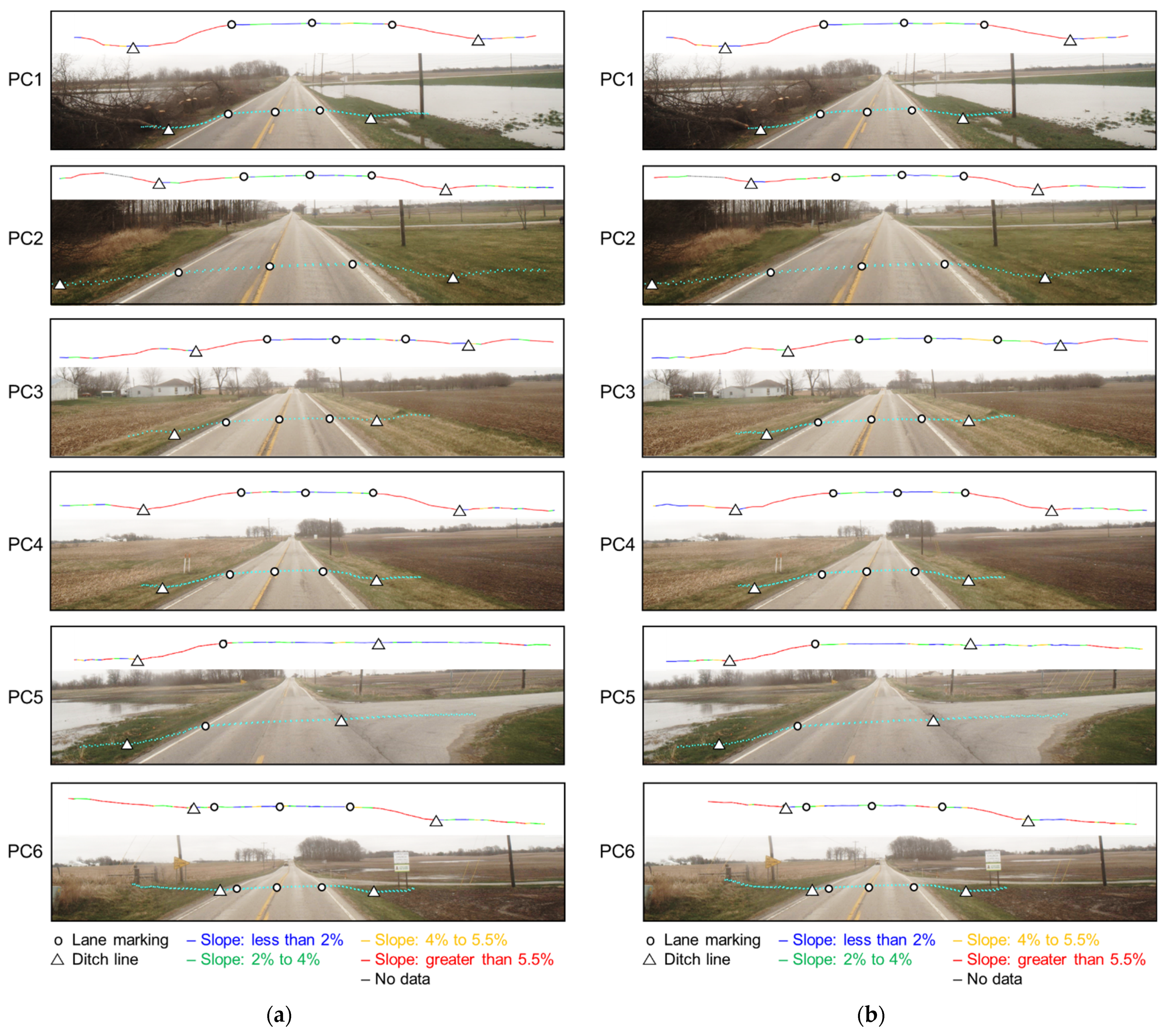
5.3. Ditch Line Characterization Using LiDAR Data

The previous section concluded that the PWMMS-HA and Mobile-pack are more appropriate for capturing roadside ditches. In this experiment, the proposed ditch line characterization was tested using data acquired by the two systems: datasets C-1 (collected by PWMMS-HA) and C-2 (collected by Mobile-pack). The results for the one-mile-long ROI are presented in this section, showing:

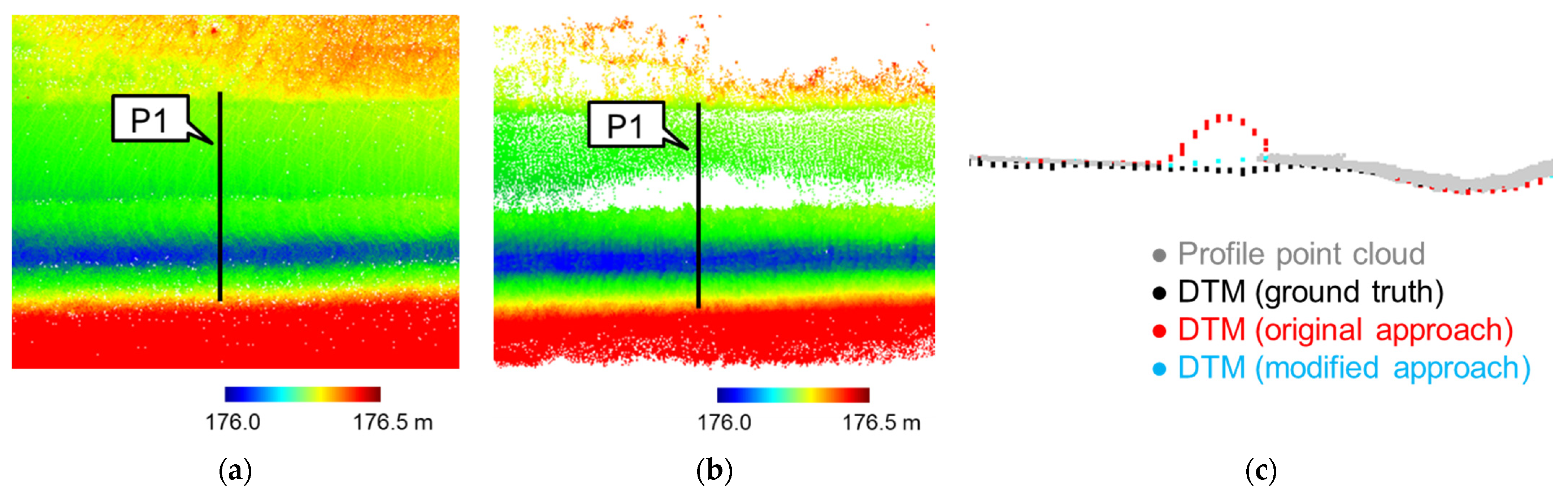
• bare earth point cloud and corresponding DTM;
• cross-sectional profiles in 3D and 2D, together with the slope evaluation results; and
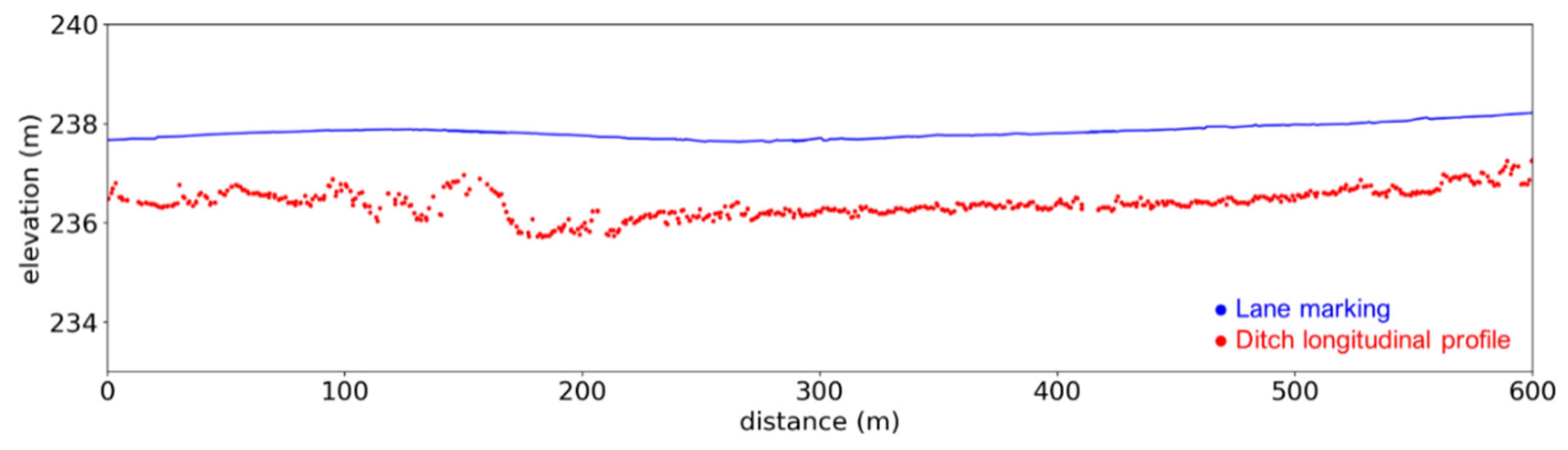
• drainage network and longitudinal profiles.

Upon reconstructing the point cloud, the bare earth point cloud and DTM were generated for each MLMS dataset using the modified cloth simulation approach, and the corresponding point density map was derived based on the bare earth point cloud. Figure 17 show the point cloud (with trajectory), bare earth point cloud, DTM, and point density map (with trajectory) from PWMMS-HA and Mobile-pack over an area covering location PC2 (see Figure 4). The bare earth point cloud is a subset of the point cloud, and therefore a non-uniform distribution of the points can be observed (see Figure 17b). The DTM is a rasterized dataset and therefore has a uniform distribution within the ROI. In Figure 17c, the DTM based on the modified cloth simulation approach captures the terrain even though there are some gaps in the point cloud. Prior to ditch line characterization, we inspected the point density of the bare earth point cloud (Figure 17d) from the two MLMS units. For both systems, the point density decreases as the distance from the trajectory increases. The degradation in point density for Mobile-pack is much larger than that of the PWMMS-HA. This is mainly related to the LiDAR unit orientation on the platforms, as we noted earlier. As shown in Figure 17d, PWMMS-HA has a decent point density up to 20 m to the left and right of the road edge. Mobile-pack, on the other hand, mainly covers an area within 6 m from the road edge. In this study site, the roadside ditches are typically present within 5 m from the road edge. Therefore, both systems have full coverage over the ditches for subsequent analysis. Another pattern that can be observed from the Mobile-pack point density map is the consistently lower point density westbound compared to eastbound. This is a result of the different driving speeds—50 mph westbound and 30 mph eastbound.

Cross-sectional profiles at locations PC1, PC2, PC3, and PC4 were extracted, and the slope along each profile was calculated. Sample results showing profile PC2 are visualized in Figure 18. The profile side view shown in Figure 18a demonstrates that the LiDAR points were able to penetrate the vegetation and capture points below the canopy. The PWMMS-HA produces a denser point cloud as compared to the Mobile-pack, yet the DTMs derived from both systems are compatible. The results indicate that the modified cloth simulation approach can produce a reliable terrain model as long as we have a sufficient number of points over the ROI. The slope along the profile was calculated based on the DTM points. Figure 18b depicts the profile PC2 colored by the slope along with lane markings (detected based on the approach proposed by Cheng et al. [13]) that signify the road boundaries. The slope evaluation results from the two MLMS units are consistent with the standard values: 2% on driving lanes, 4% on the shoulder, and 6-by-1 gradation for ditch lines. Figure 18c shows the back-projected DTM points on an image captured by the front left camera onboard the PWMMS-HA. The back-projected points coincide with the corresponding features in the image, which verifies the reliability of the system calibration.

The hydrological analyses including flow direction and flow accumulation were performed using ESRI’s ArcGIS [65]. Figure 19 depicts the drainage network map together with the detected lane markings, using the bare earth point cloud as a base map. As can be seen in the figure, the drainage networks are aligned well with the ‘valley’ of the ditches. Subsequently, longitudinal profiles were extracted from the drainage network by connecting major streams and removing tributaries. Figure 20 visualizes the longitudinal profiles and the lane markings on the left and right side of the road (when driving eastbound) where the green line, red line, and blue line are the profile from PWMMS-HA, profile from Mobile-pack, and detected lane marking, respectively. The longitudinal profiles extracted from the PWMMS-HA and Mobile-pack data are compatible, as the green and red lines are almost aligned with each other. Moreover, the grade of the ditch line follows the grade of the road, and the elevation of the ditch line is consistently lower than the road centerline. Six cross-sectional profiles at locations PC1 to PC6 were also extracted and visualized in Figure 21, both in 3D and 2D. Profiles at locations PC1, PC2, PC3, and PC4 (see Figure 4) were extracted at an interval of 400 m. Locations PC5 and PC6 show areas where the elevation of the ditch line is very close to that of the road edge line, as can be seen in Figure 20. Based on the 2D and 3D visualization shown in Figure 21, location PC5 is an intersection and thus there is no ditch on the right side of the road. Location PC6 shows an area where the ditch on the left side of the road is very shallow and can barely be seen.

The strength of MLMS units for characterizing roadside ditches lies in the ability to (i) visualize the profiles in 3D point clouds as well as 2D images, and (ii) incorporate other information derived from MLMS data (for example, the detected lane markings). Such capability leads to a thorough understanding of roadside drainage conditions, which is the key to prioritizing and planning maintenance. In addition, with the proposed ditch line characterization approach, the relatively low-cost system (Mobile-pack) can achieve similar performance as compared to PWMMS-HA.

In this section, the performance of PWMMS-HA and Mobile-pack for roadside ditch characterization was evaluated. The advantage of PWMMS-HA is that the point cloud has a more uniform density and a larger coverage (up to 20 m from the road edge). That is, in addition to the roadside ditches, the PWMMS-HA point cloud can provide information on the areas adjacent to the ditches. Such information is helpful for investigating the causes of local flooding. Nevertheless, both PWMMS-HA and Mobile-pack point clouds have adequate spatial coverage for ditch line characterization. The cross-sectional profiles, drainage network, and longitudinal profiles extracted from both MLMS units are shown to be compatible.

6. Discussion

6.1. Comparative Performance of Different MLMS Units

In this study, the performance of five alternative MLMS units, including UAV, UGV, Backpack, Mobile-pack, PWMMS-HA, and PWMMS-UHA, was evaluated.

Table 10. Comparison of different MLMS units showing their merits and shortcomings.

System	Platform	Pros	Cons
UAV	Aerial	Bird’s-eye view (good for areas with mild slope) Uniform point density Can maneuver over areas that are difficult to reach by ground vehicles Relatively low-cost	Prone to occlusions by canopy cover Relatively low point density
UGV	Wheel-based	High point density Relatively low-cost	Prone to occlusions by terrain Large variation in point density Not practical for mapping long extent
Backpack	Portable	High point density Relatively low-cost	Prone to occlusions by terrain Large variation in point density Not practical for mapping long extent
Mobile-pack	Wheel-based	High point density Can travel at a higher speed and cover a longer extent Relatively low-cost	Prone to occlusions by terrain Large variation in point density
PWMMS-HA	Wheel-based	High point density Can travel at a higher speed and cover a longer extent	Prone to occlusions by terrain Large variation in point density Expensive
PWMMS-UHA	Wheel-based	High point density Can travel at a higher speed and cover a longer extent	Prone to occlusions by terrain Large variation in point density Expensive

summarizes these MLMS units along with their merits and shortcomings. The main difference between aerial and ground systems is the view angle. The aerial systems are less prone to occlusions by terrain and have a relatively uniform point density. However, canopy cover (especially those caused by trees) is the main limitation. More specifically, UAV LiDAR may not have adequate penetration to the ground to capture ditches that are below the dense canopy. Ground systems, in contrast, are more likely to suffer from occlusions caused by terrain and above-ground objects. The point density from ground systems varies based on the sensor-to-object distance. However, the impact of canopy cover is less. In terms of field survey, aerial systems can maneuver over areas that are difficult to reach with ground vehicles. Currently, UAV surveys are limited to a relatively small coverage area due to line-of-sight regulations. Nonetheless, with the ever-changing technology as well as aviation-related policies, the possibility for UAVs to operate over a broader range is not unforeseeable. Among the ground systems, wheel-based systems that can travel at a higher speed and cover a longer extent are more practical for field surveys. Considering the cost of the systems, the Mobile-pack is the most cost-effective solution for ditch mapping.

6.2. Potential of Mobile LiDAR Data for Flooded Region Detection and Flood Risk Assessment

Standing water is an indication of drainage issues/high flooding risk. Therefore, the ability to identify such areas is critical for prioritizing and planning maintenance. Based on the hypothesis that LiDAR has zero return over water bodies, flooded regions can be identified by detecting areas where LiDAR points are absent. With the ability of 2D–3D cross-visualization, the reported ROIs can be visualized both in 3D point cloud and 2D images. An example of potential flooded region detection and visualization is shown in Figure 22. The image-based visualization helps to associate any environmental factors that lead to flooding. Moreover, with the proposed modified cloth simulation approach, a reliable, high-resolution DTM can be generated. This DTM serves as a key element for hydrological analyses and facilitates flood risk assessment.

7. Conclusions and Recommendations for Future Work

This paper presented an evaluation and application of mobile LiDAR in mapping roadside ditches for slope and drainage analyses. The performance of different grades of mobile LiDAR mapping systems was assessed in terms of spatial coverage, relative vertical accuracy, and absolute vertical accuracy. All the systems have complete spatial coverage over the roadside ditches with sufficient drive-runs/flight lines. Point clouds from different MLMS units, including an unmanned aerial vehicle, an unmanned ground vehicle, a portable backpack system along with its vehicle-mounted version, a medium-grade wheel-based system, and a high-grade wheel-based system, are in agreement within a ±3 cm range along the vertical direction. The absolute vertical accuracy for all the MLMS units was found to be ±3 cm for solid surfaces and ±7 cm for vegetated areas. Field surveys with the wheel-based and vehicle-mounted portable systems are more efficient and can be scaled up to cover a large area that is impractical with UAV, UGV, and backpack surveys. To an even greater extent, the low cost of the vehicle-mounted portable system in contrast to the more sophisticated platforms, the medium-grade and high-grade wheel-based systems, makes the former even more justifiable for its application in ditch line mapping.

A framework for ditch line characterization, including (i) cross-sectional profile extraction, visualization, and slope evaluation and (ii) drainage network and longitudinal profile extraction, is proposed and tested using datasets acquired by the medium-grade wheel-based and vehicle-mounted portable systems. An existing ground-filtering approach, cloth simulation, is modified to handle variations in point density of the mobile LiDAR data. Drainage analysis was conducted to identify ditch lines and detect any potential drainage issues. The cross-sectional/longitudinal profiles of the ditch were automatically extracted from LiDAR data and visualized in both the 2D image and 3D point cloud. The slope along the profile was calculated, reported, and compared to standard values. These results, when combined with other information derived from MLMS data, lead to a thorough understanding of highway conditions, which is helpful for planning highway maintenance. If multi-date datasets are available, the proposed framework can be implemented to identify changes in the 2D location as well as the elevation/slope of the ditches. This can signal the presence of sediments/debris in the ditch or the erosion of the ditch line material.

Currently, our analysis is solely based on topographic data. In the future, it is possible to incorporate weather and hydrological data and perform flood simulation to identify areas with flooding risk. Future research will also focus on comparative analysis of mapped ditch profiles and as-built drawings, which would signify how the mapped profiles deviate from the designed profiles. Furthermore, for all the MLMS units discussed in this study, in particular, the vehicle-mounted portable system, owing to its portability, one of the future activities will investigate different orientation options of the LiDAR unit to achieve optimized coverage (and point density) of roadside ditches while maximizing the data acquisition throughput of the MLMS.

References

1. Buchanan, B.; Easton, Z.M.; Schneider, R.L.; Walter, M.T. Modeling the hydrologic effects of roadside ditch networks on receiving waters. J. Hydrol. 2013, 486, 293–305. [Google Scholar] [CrossRef]
2. Schneider, R.; Orr, D.; Johnson, A. Understanding Ditch Maintenance Decisions of Local Highway Agencies for Improved Water Resources across New York State. Transp. Res. Rec. 2019, 2673. [Google Scholar] [CrossRef]
3. Matos, J.A. Improving Roadside Ditch Maintenance Practices in Ohio. Master’s Thesis, University of Cincinnati, Cincinnati, OH, USA, 2016. [Google Scholar]
4. Gharaibeh, N.G.; Lindholm, D.B. A condition assessment method for roadside assets. Struct. Infrastruct. Eng. 2014, 10, 409–418. [Google Scholar] [CrossRef]
5. Oti, I.C.; Gharaibeh, N.G.; Hendricks, M.D.; Meyer, M.A.; Van Zandt, S.; Masterson, J.; Horney, J.A.; Berke, P. Validity and Reliability of Drainage Infrastructure Monitoring Data Obtained from Citizen Scientists. J. Infrastruct. Syst. 2019, 25, 04019018. [Google Scholar] [CrossRef]
6. Hendricks, M.D.; Meyer, M.A.; Gharaibeh, N.G.; Van Zandt, S.; Masterson, J.; Cooper, J.T.; Horney, J.A.; Berke, P. The development of a participatory assessment technique for infrastructure: Neighborhood-level monitoring towards sustainable infrastructure systems. Sustain. Cities Soc. 2018, 38, 265–274. [Google Scholar] [CrossRef] [PubMed]
7. Costabile, P.; Costanzo, C.; De Lorenzo, G.; De Santis, R.; Penna, N.; Macchione, F. Terrestrial and airborne laser scanning and 2-D modelling for 3-D flood hazard maps in urban areas: New opportunities and perspectives. Environ. Model. Softw. 2021, 135, 104889. [Google Scholar] [CrossRef]
8. Siegel, Z.S.; Kulp, S.A. Superimposing height-controllable and animated flood surfaces into street-level photographs for risk communication. Weather. Clim. Extrem. 2021, 32, 100311. [Google Scholar] [CrossRef]
9. Levavasseur, F.; Lagacherie, P.; Bailly, J.S.; Biarnès, A.; Colin, F. Spatial modeling of man-made drainage density of agricultural landscapes. J. Land Use Sci. 2015, 10, 256–276. [Google Scholar] [CrossRef] [Green Version]
10. Roelens, J.; Höfle, B.; Dondeyne, S.; Van Orshoven, J.; Diels, J. Drainage ditch extraction from airborne LiDAR point clouds. ISPRS J. Photogramm. Remote. Sens. 2018, 146, 409–420. [Google Scholar] [CrossRef]
11. Ariza-Villaverde, A.B.; Jiménez-Hornero, F.J.; Gutiérrez de Ravé, E. Influence of DEM resolution on drainage network extraction: A multifractal analysis. Geomorphology 2015, 241, 243–254. [Google Scholar] [CrossRef]
12. Metz, M.; Mitasova, H.; Harmon, R.S. Efficient extraction of drainage networks from massive, radar-based elevation models with least cost path search. Hydrol. Earth Syst. Sci. 2011, 15, 667–678. [Google Scholar] [CrossRef] [Green Version]
13. Cheng, Y.T.; Patel, A.; Wen, C.; Bullock, D.; Habib, A. Intensity thresholding and deep learning based lane marking extraction and lanewidth estimation from mobile light detection and ranging (LiDAR) point clouds. Remote Sens. 2020, 12, 1379. [Google Scholar] [CrossRef]
14. Wen, C.; Sun, X.; Li, J.; Wang, C.; Guo, Y.; Habib, A. A deep learning framework for road marking extraction, classification and completion from mobile laser scanning point clouds. ISPRS J. Photogramm. Remote Sens. 2019, 147, 178–192. [Google Scholar] [CrossRef]
15. Cai, H.; Rasdorf, W. Modeling road centerlines and predicting lengths in 3-D using LIDAR point cloud and planimetric road centerline data. Comput. Civ. Infrastruct. Eng. 2008, 23, 157–173. [Google Scholar] [CrossRef]
16. Lin, Y.C.; Cheng, Y.T.; Lin, Y.J.; Flatt, J.E.; Habib, A.; Bullock, D. Evaluating the Accuracy of Mobile LiDAR for Mapping Airfield Infrastructure. Transp. Res. Rec. 2019, 2673, 117–124. [Google Scholar] [CrossRef]
17. Ravi, R.; Habib, A.; Bullock, D. Pothole mapping and patching quantity estimates using lidar-based mobile mapping systems. Transp. Res. Rec. 2020, 2674, 124–134. [Google Scholar] [CrossRef]
18. You, C.; Wen, C.; Member, S.; Wang, C.; Member, S.; Li, J.; Member, S.; Habib, A. Joint 2-D–3-D Traffic Sign Landmark Data Set for Geo-Localization Using Mobile Laser Scanning Data. IEEE Trans. Intell. Transp. Syst. 2018, 20, 2550–2565. [Google Scholar] [CrossRef]
19. Soilán, M.; Riveiro, B.; Martínez-Sánchez, J.; Arias, P. Traffic sign detection in MLS acquired point clouds for geometric and image-based semantic inventory. ISPRS J. Photogramm. Remote Sens. 2016, 114, 92–101. [Google Scholar] [CrossRef]
20. Castro, M.; Lopez-Cuervo, S.; Paréns-González, M.; de Santos-Berbel, C. LIDAR-based roadway and roadside modelling for sight distance studies. Surv. Rev. 2016, 48, 309–315. [Google Scholar] [CrossRef]
21. Gargoum, S.A.; El-Basyouny, K.; Sabbagh, J. Assessing Stopping and Passing Sight Distance on Highways Using Mobile LiDAR Data. J. Comput. Civ. Eng. 2018, 32, 04018025. [Google Scholar] [CrossRef]
22. Gong, J.; Zhou, H.; Gordon, C.; Jalayer, M. Mobile terrestrial laser scanning for highway inventory data collection. Comput. Civ. Eng. 2012, 2012, 545–552. [Google Scholar]
23. Jalayer, M.; Gong, J.; Zhou, H.; Grinter, M. Evaluation of Remote Sensing Technologies for Collecting Roadside Feature Data to Support Highway Safety Manual Implementation. J. Transp. Saf. Secur. 2015, 7, 345–357. [Google Scholar] [CrossRef]
24. Gargoum, S.; El-Basyouny, K. Automated extraction of road features using LiDAR data: A review of LiDAR applications in transportation. In Proceedings of the 2017 4th International Conference on Transportation Information and Safety (ICTIS), Banff, AB, Canada, 8–10 August 2017; pp. 563–574. [Google Scholar] [CrossRef]
25. Williams, K.; Olsen, M.J.; Roe, G.V.; Glennie, C. Synthesis of Transportation Applications of Mobile LIDAR. Remote Sens. 2013, 5, 4652–4692. [Google Scholar] [CrossRef] [Green Version]
26. Guan, H.; Li, J.; Cao, S.; Yu, Y. Use of mobile LiDAR in road information inventory: A review. Int. J. Image Data Fusion 2016, 7, 219–242. [Google Scholar] [CrossRef]
27. Tsai, Y.; Ai, C.; Wang, Z.; Pitts, E. Mobile cross-slope measurement method using lidar technology. Transp. Res. Rec. 2013, 2367, 53–59. [Google Scholar] [CrossRef]
28. Holgado-Barco, A.; Riveiro, B.; González-Aguilera, D.; Arias, P. Automatic Inventory of Road Cross-Sections from Mobile Laser Scanning System. Comput. Civ. Infrastruct. Eng. 2017, 32, 3–17. [Google Scholar] [CrossRef] [Green Version]
29. Puente, I.; Akinci, B.; González-Jorge, H.; Díaz-Vilariño, L.; Arias, P. A semi-automated method for extracting vertical clearance and cross sections in tunnels using mobile LiDAR data. Tunn. Undergr. Sp. Technol. 2016, 59, 48–54. [Google Scholar] [CrossRef]
30. Levavasseur, F.; Bailly, J.S.; Lagacherie, P.; Colin, F.; Rabotin, M. Simulating the effects of spatial configurations of agricultural ditch drainage networks on surface runoff from agricultural catchments. Hydrol. Process. 2012, 26, 3393–3404. [Google Scholar] [CrossRef] [Green Version]
31. Barber, C.P.; Shortridge, A. Lidar elevation data for surface hydrologic modeling: Resolution and representation issues. Cartogr. Geogr. Inf. Sci. 2005, 32, 401–410. [Google Scholar] [CrossRef]
32. Ibeh, C.; Pallai, C.; Saavedra, D. Lidar-based roadside ditch mapping in York and Lancaster Counties. Pennsylvania. pp. 1–17. Available online: https://www.chesapeakebay.net/documents/Lidar-Based_Roadside_Ditch_Mapping_Report.pdf (accessed on 22 June 2021).
33. Bertels, L.; Houthuys, R.; Sterckx, S.; Knaeps, E.; Deronde, B. Large-scale mapping of the riverbanks, mud flats and salt marshes of the scheldt basin, using airborne imaging spectroscopy and LiDAR. Int. J. Remote Sens. 2011, 32, 2905–2918. [Google Scholar] [CrossRef]
34. Murphy, P.; Ogilvie, J.; Meng, F.-R.; Arp, P. Advanced Bash-Scripting Guide An in-depth exploration of the art of shell scripting Table of Contents. Hydrol. Process. 2007, 22, 1747–1754. [Google Scholar] [CrossRef]
35. Günen, M.A.; Atasever, Ü.H.; Taşkanat, T.; Beşdok, E. Usage of unmanned aerial vehicles (UAVs) in determining drainage networks. E-J. New World Sci. Acad. 2019, 14, 1–10. [Google Scholar] [CrossRef]
36. Pricope, N.G.; Halls, J.N.; Mapes, K.L.; Baxley, J.B.; Wu, J.J. Quantitative comparison of uas-borne lidar systems for high-resolution forested wetland mapping. Sensors 2020, 20, 4453. [Google Scholar] [CrossRef]
37. Yan, L.; Liu, H.; Tan, J.; Li, Z.; Chen, C. A multi-constraint combined method for ground surface point filtering from mobile LiDAR point clouds. Remote Sens. 2017, 9, 958. [Google Scholar] [CrossRef] [Green Version]
38. Serifoglu Yilmaz, C.; Yilmaz, V.; Güngör, O. Investigating the performances of commercial and non-commercial software for ground filtering of UAV-based point clouds. Int. J. Remote Sens. 2018, 39, 5016–5042. [Google Scholar] [CrossRef]
39. Bolkas, D.; Naberezny, B.; Jacobson, M.G. Comparison of sUAS Photogrammetry and TLS for Detecting Changes in Soil Surface Elevations Following Deep Tillage. J. Surv. Eng. 2021, 147, 04021001. [Google Scholar] [CrossRef]
40. Bailly, J.S.; Lagacherie, P.; Millier, C.; Puech, C.; Kosuth, P. Agrarian landscapes linear features detection from LiDAR: Application to artificial drainage networks. Int. J. Remote Sens. 2008, 29, 3489–3508. [Google Scholar] [CrossRef]
41. Rapinel, S.; Hubert-Moy, L.; Clément, B.; Nabucet, J.; Cudennec, C. Ditch network extraction and hydrogeomorphological characterization using LiDAR-derived DTM in wetlands. Hydrol. Res. 2015, 46, 276–290. [Google Scholar] [CrossRef]
42. Broersen, T.; Peters, R.; Ledoux, H. Automatic identification of watercourses in flat and engineered landscapes by computing the skeleton of a LiDAR point cloud. Comput. Geosci. 2017, 106, 171–180. [Google Scholar] [CrossRef] [Green Version]
43. Roelens, J.; Rosier, I.; Dondeyne, S.; Van Orshoven, J.; Diels, J. Extracting drainage networks and their connectivity using LiDAR data. Hydrol. Process. 2018, 32, 1026–1037. [Google Scholar] [CrossRef]
44. Balado, J.; Martínez-Sánchez, J.; Arias, P.; Novo, A. Road environment semantic segmentation with deep learning from mls point cloud data. Sensors 2019, 19, 3466. [Google Scholar] [CrossRef] [Green Version]
45. Applanix POSLV 220 Datasheet. Available online: https://www.applanix.com/products/poslv.htm (accessed on 26 April 2020).
46. Applanix APX-15 Datasheet. Available online: https://www.applanix.com/products/dg-uavs.htm (accessed on 26 April 2020).
47. Novatel IMU-ISA-100C. Available online: https://docs.novatel.com/OEM7/Content/Technical_Specs_IMU/ISA_100C_Overview.htm (accessed on 26 April 2020).
48. Novatel SPAN-CPT. Available online: https://novatel.com/support/previous-generation-products-drop-down/previous-generation-products/span-cpt (accessed on 26 May 2021).
49. Novatel SPAN-IGM-A1. Available online: https://novatel.com/support/span-gnss-inertial-navigation-systems/span-combined-systems/span-igm-a1 (accessed on 26 May 2021).
50. Velodyne Puck Hi-Res Datasheet. Available online: https://velodynelidar.com/products/puck-hi-res/ (accessed on 26 May 2021).
51. Velodyne HDL32E Datasheet. Available online: https://velodynelidar.com/products/hdl-32e/ (accessed on 26 May 2021).
52. Riegl VUX-1HA. Available online: http://www.riegl.com/products/newriegl-vux-1-series/newriegl-vux-1ha (accessed on 26 April 2020).
53. Z+F Profiler 9012. Available online: https://www.zf-laser.com/Z-F-PROFILER-R-9012.2d_laserscanner.0.html (accessed on 26 April 2020).
54. Velodyne Ultra Puck Datasheet. Available online: https://velodynelidar.com/products/ultra-puck/ (accessed on 26 May 2021).
55. Ravi, R.; Lin, Y.J.; Elbahnasawy, M.; Shamseldin, T.; Habib, A. Simultaneous system calibration of a multi-LiDAR multi-camera mobile mapping platform. IEEE J. Sel. Top. Appl. Earth Obs. Remote Sens. 2018, 11, 1694–1714. [Google Scholar] [CrossRef]
56. Habib, A.; Lay, J.; Wong, C. LIDAR Error Propagation Calculator. Available online: https://engineering.purdue.edu/CE/Academics/Groups/Geomatics/DPRG/files/LIDARErrorPropagation.zip (accessed on 23 June 2021).
57. Zhang, W.; Qi, J.; Wan, P.; Wang, H.; Xie, D.; Wang, X.; Yan, G. An easy-to-use airborne LiDAR data filtering method based on cloth simulation. Remote Sens. 2016, 8, 501. [Google Scholar] [CrossRef]
58. Lin, Y.C.; Habib, A. Quality control and crop characterization framework for multi-temporal UAV LiDAR data over mechanized agricultural fields. Remote Sens. Environ. 2021, 256, 112299. [Google Scholar] [CrossRef]
59. Lague, D.; Brodu, N.; Leroux, J. Accurate 3D comparison of complex topography with terrestrial laser scanner: Application to the Rangitikei canyon (N-Z). ISPRS J. Photogramm. Remote Sens. 2013, 82, 10–26. [Google Scholar] [CrossRef] [Green Version]
60. Renaudin, E.; Habib, A.; Kersting, A.P. Featured-based registration of terrestrial laser scans with minimum overlap using photogrammetric data. ETRI J. 2011, 33, 517–527. [Google Scholar] [CrossRef]
61. Ravi, R.; Habib, A. Least squares adjustment with a rank-deficient weight matrix and its applicability towards image/LiDAR data processing. Photogramm. Eng. Remote Sens. 2021, in press. [Google Scholar]
62. McGee, H.W.; Nabors, D.; Baughman, T. Maintenance of Drainage Features for Safety: A Guide for Street and Highway Maintenance Personnel (No. FHWA-SA-09-024); United States. Federal Highway Administration: Washington, DC, USA, 2009. [Google Scholar]
63. Jenson, S.K.; Domingue, J.O. Extracting topographic structure from digital elevation data for geographic information system analysis. Photogramm. Eng. Remote Sens. 1988, 54, 1593–1600. [Google Scholar]
64. Fischler, M.A.; Bolles, R.C. Random Sample Paradigm for Model Consensus: A Apphcatlons to Image Fitting with Analysis and Automated Cartography. Graph. Image Process. 1981, 24, 381–395. [Google Scholar] [CrossRef]
65. Maidment, D.R.; Morehouse, S. Arc Hydro: GIS for Water Resources; ESRI, Inc.: Redlands, CA, USA, 2002. [Google Scholar]
Figure 1. MLMS units used in this study: (a) unmanned aerial vehicle (UAV), (b) unmanned ground vehicle (UGV), (c) Backpack, (d) Mobile-pack, (e) medium-grade system (PWMMS-HA), and (f) high-grade system (PWMMS-UHA). All of these platforms are non-commercial systems designed and integrated by the research group.
Remotesensing 13 02485 g001aRemotesensing 13 02485 g001b
Figure 2. Study site at CR500N: (a) the surveyed area and cross-section location PA1 (aerial photo adapted from a Google Earth Image), and (b) image of the surveyed area at location PA1 captured by one of the cameras onboard the PWMMS-HA.
Remotesensing 13 02485 g002aRemotesensing 13 02485 g002b
Figure 3. Study site at McCormick Rd: (a) surveyed area and cross-section locations PB1, PB2, PB3, and PB4 (aerial photo adapted from a Google Earth image), and (b) image of the surveyed area at location PB3 captured by one of the cameras onboard the PWMMS-HA.
Remotesensing 13 02485 g003aRemotesensing 13 02485 g003b
Figure 4. Study site at SR28: (a) the one-mile-long region of interest and cross-section locations PC1, PC2, PC3, and PC4 (aerial photo adapted from a Google Earth Image), and (b) image of the surveyed area at location PC1 captured by one of the cameras onboard the PWMMS-HA.
Remotesensing 13 02485 g004
Figure 5. Main steps of the proposed framework for point cloud quality assessment and ditch mapping/characterization.
Remotesensing 13 02485 g005
Figure 6. Comparison between the original and modified approaches for digital terrain model (DTM) generation: (a) point cloud from PWMMS-HA, (b) point cloud from UGV, and (c) side view of profile P1 showing point cloud, ground truth DTM, and DTM based on the original and modified approaches.
Remotesensing 13 02485 g006
Figure 7. An example of cross-sectional profile colored by slope.
Remotesensing 13 02485 g007
Figure 8. Longitudinal profile extraction showing top view of: (a) drainage network, (b) drainage network after removing tributaries, and (c) streamlines after outlier removal.
Remotesensing 13 02485 g008aRemotesensing 13 02485 g008b
Figure 9. An example of a longitudinal profile together with the detected lane marking.
Remotesensing 13 02485 g009
Figure 10. MLMS mapping products showing the (a) point cloud and trajectory and (b) bare earth point cloud from UAV, PWMMS-HA, and Mobile-pack.
Remotesensing 13 02485 g010
Figure 11. Side view of a cross-sectional profile at location PA1 showing the original and bare earth point clouds from (a) UAV, (b) PWMMS-HA, and (c) Mobile-pack.
Remotesensing 13 02485 g011aRemotesensing 13 02485 g011b
Figure 12. Point density of the bare earth point cloud along with the trajectory from UAV, PWMMS-HA, and Mobile-pack.
Remotesensing 13 02485 g012
Figure 13. Cross-sectional profiles at location PB3 from different systems showing the side view, top view, and the platform tracks (black dashed lines).
Remotesensing 13 02485 g013
Figure 14. Cross-sectional profiles at locations PB1, PB2, PB3, and PB4 from different systems showing the side view of the bare earth point cloud together with a one-meter-long zoom-in view over the road surface and ditch.
Remotesensing 13 02485 g014
Figure 15. Cross-sectional profile at location PB3 showing the point cloud, DTM, and real-time kinematic global navigation satellite systems (RTK-GNSS) survey points.
Remotesensing 13 02485 g015
Figure 16. Statistics of elevation difference between RTK-GNSS surveyed points and LiDAR points for (a) PWMMS-HA, (b) PWMMS-UHA, (c) UGV, (d) Backpack, and (e) Mobile-pack with residual plots of range, 25th percentile, median, and 75th percentile.
Remotesensing 13 02485 g016
Figure 17. LiDAR-based products from PWMMS-HA and Mobile-pack (showing an 80-m long area near location PC2): (a) point cloud and trajectory, (b) bare earth point cloud, (c) digital terrain model (DTM), and (d) point density of the bare earth point cloud and trajectory.
Remotesensing 13 02485 g017
Figure 18. Cross-sectional profile at location PC2: (a) point cloud and DTM profiles, (b) slope evaluation results together with lane marking points, and (c) image with back-projected DTM and lane marking points. The lane marking points are extracted from the point cloud using the approach proposed by Cheng et al. [13].
Remotesensing 13 02485 g018aRemotesensing 13 02485 g018b
Figure 19. Drainage network (in black) together with detected lane markings (in blue) superimposed on the bare earth point cloud (colored by height).
Remotesensing 13 02485 g019
Figure 20. Longitudinal profiles from PWMMS-HA and Mobile-pack data together with the detected lane marking showing: (a) the ditch and road edge line on the left and (b) the ditch and road edge line on the right when driving eastbound.
Remotesensing 13 02485 g020
Figure 21. Cross-sectional profiles shown in 3D (side view and colored by slope) and the images from (a) PWMMS-HA and (b) Mobile-pack.
Remotesensing 13 02485 g021
Figure 22. An example of potential flooded region visualized in: (a) 3D point cloud and (b) 2D image.
Remotesensing 13 02485 g022