Abstract
Building boundary optimization is an essential post-process step for building extraction (by image classification). However, current boundary optimization methods through smoothing or line fitting principles are unable to optimize complex buildings. In response to this limitation, this paper proposes an object-oriented building contour optimization method via an improved generalized gradient vector flow (GGVF) snake model and based on the initial building contour results obtained by a classification method. First, to reduce interference from the adjacent non-building object, each building object is clipped via their extended minimum bounding rectangles (MBR). Second, an adaptive threshold Canny edge detection is applied to each building image to detect the edges, and the progressive probabilistic Hough transform (PPHT) is applied to the edge result to extract the line segments. For those cases with missing or wrong line segments in some edges, a hierarchical line segments reconstruction method is designed to obtain complete contour constraint segments. Third, accurate contour constraint segments for the GGVF snake model are designed to quickly find the target contour. With the help of the initial contour and constraint edge map for GGVF, a GGVF force field computation is executed, and the related optimization principle can be applied to complex buildings. Experimental results validate the robustness and effectiveness of the proposed method, whose contour optimization has higher accuracy and comprehensive value compared with that of the reference methods. This method can be used for effective post-processing to strengthen the accuracy of building extraction results.
1. Introduction
Building extraction from high-resolution remote sensing images plays a key role in mapping, city planning and management, and disaster damage analysis and response. Classification is an important building extraction method that employs the traditional machine learning principle [1,2] and deep learning [3,4]. However, given the presence of shadows and vegetation occlusion, the interference of similar spectra, and the complexity of building structures, the building extraction results are often irregular [5,6] and fail to meet real application requirements. Meanwhile, many researchers have focused on improving building extraction accuracy than optimizing building contours. Therefore, designing an optimization method that can enhance the similarity between building detection results and real building shapes has become imperative.
The optimization methods adopted by researchers mainly include the dominant direction method, the bounding rectangle method, and the active contour model method.
The first category of regularized building boundary extraction methods is based on the prevailing building direction. Lee et al. [7] proposed an optimized method by making up a building with regular grids. First, the straight-line segments identified via Hough transformation were obtained based on the initial building results derived from the classification. Second, a grid was constructed by acquiring the dominant line and the line that is parallel and perpendicular to the dominant line. Third, after calculating the building proportion in each grid cell and judging which cell belongs to the building, the building is reconstructed by using those grid cells that meet the specified conditions. Albert et al. [8] used the alpha shape algorithm to obtain the initial building contour. The building dominant direction and line segments were extracted via Hough transformation and were combined with the corner points to obtain a regular contour via energy minimization. Similarly, based on the hypothesis that the adjacent building edges are perpendicular to one another, the hierarchical least-squares solution was applied in building contour optimization [9]. Initially, relatively long line segments were extracted from the building boundary, and their least-squares solution was determined under the assumption that these long line segments lie in two mutually perpendicular directions. In the next step, all line segments were included to determine the least-squares solution by using the slopes of the long line segments as weighted approximations. Partovi et al. [10] adopted the random sampling consistent method to fit those building edges with more than vertical correlation. Ding et al. [11] grouped the corner points and applied the least-squares method to fit each group of corner points into a straight line. After rotating the straight-line segments to be perpendicular or parallel to the dominant building direction, the building was regularized by connecting the intersection points of adjacent line segments. Although these methods regularize the building boundary to a certain extent, they have high requirements for initial building results. When the initial result is not good enough, these regularization methods lack the ability to further judge the real physical boundary of the building and can only reduce the serration segments on the contour boundary.
The second category of regularized building boundary extraction methods is based on MBR. By viewing a building as a group of rectangles, Kwak et al. [12] decomposed the initial building results into different rectangular parts, obtained their MBRs, and regularized the building by reconstructing these MBRs. However, when vegetation or other non-building objects surrounding a building are incorrectly classified as a building, the MBR edges would not be fitted with the real building edge, thereby leading to an inaccurate optimization. To solve this problem, Feng et al. [13] used topological rules to check whether the building edge is occluded by vegetation. The edge points in a line were then used to optimize the occluded edge. This method efficiently handles the occlusion problem and improves the integrity of building extraction. Chang et al. [14] used the Hausdorff distance algorithm to evaluate the similarity between the building and MBR boundaries. The coordinate of the relative MBR boundary was then used to replace the partial boundary that was similar to MBR. For those boundary parts not optimized by these methods, the corner points were detected, filtered, and reconnected for regularization. While these methods can further optimize building boundaries, they have more stringent requirements for the shape of buildings. These methods can only be used to optimize rectangular or rectangular combination buildings with right angles. Moreover, they cannot be well regularized for buildings with non-right angle or arc features.
The third category of regularized building boundary extraction methods is based on an active contour model [15]. Specifically, these methods combine the low-level image information with high-level prior knowledge to extract and optimize buildings. Peng et al. [16] designed an improved snake model that combined radiation features with context information to optimize building boundaries. They obtained satisfactory results in their experiments in dense urban areas. Ahmadi et al. [17] explored an active contour model that extracts the building boundary based on a contour set formula. They also used the HSV components to modify the traditional active contour segmentation model for building extraction. To extract buildings from imageries and LiDAR point cloud data, the active contour model is often used to improve the completeness and correctness of building results [18,19]. Those methods based on the active contour model are not limited by the shape of buildings, thereby supporting the reliability and practicability of the active contour model in the optimization of building extraction. However, some problems need to be addressed when using the active contour model. For example, this model requires a manual setting of the initial contour, and the concave boundary does not converge to the actual edge.
In sum, the current methods rely on the initial results, which are limited by the regularized building shape and the active contour model itself. In response to optimizing the building contour to make it closer to the actual physical shape, this paper develops an object-oriented building contour optimization method for image classification results obtained via the GGVF snake model [20]. First, based on the initial building outlines extracted by classification, the extended MBR clips the original image to obtain a single building sub-image, thereby reducing the subsequent computational load and global impact. Afterward, based on the GGVF snake model, an improved strategy is developed to enhance adjustability. On the one hand, the initial building boundary is corroded and used as the GGVF initial contour. On the other hand, accurate contour constraint segments for the GGVF snake model are designed to rapidly identify the target contour. Next, adaptive threshold Canny edge detection and PPHT [21] are then used to obtain an accurate and adjustable contour edge map. Finally, after computing the GGVF force field, the improved edge map is used to quickly minimize the energy function down to the building constraint contour to obtain the final optimized contour.
The main highlights of this work are summarized as follows:
- (1)
- This study adopts an object-oriented optimization strategy to reduce the interference from adjacent objects. The single building image after clipping can make the optimization focused on the building, reduce the impact of other adjacent objects, and greatly decrease the amount of calculations.
- (2)
- An improved GGVF snake model is designed by automatically obtaining the initial contour and constraint edge map. The initial contour is modified from the classification results, and the constraint edge map is extracted effectively via the improved Canny detector and Hough transformation. The proposed method is not limited by the building shape and size and has strong robustness.
2. Methodology
The GGVF snake model can transform an active contour convergence into long, thin indentations (LTIs) and maintain the other desirable properties of gradient vector flow (GVF) [22], such as its extended capture range. Therefore, this model is useful in optimizing the building active contour. However, the initial seed points and edge map are vital factors in model convergence. This paper designs a strategy for automatically providing effective initial seed information and edge map. Based on the GGVF model and the promoted strategy, the building contour can be optimized accurately and automatically.
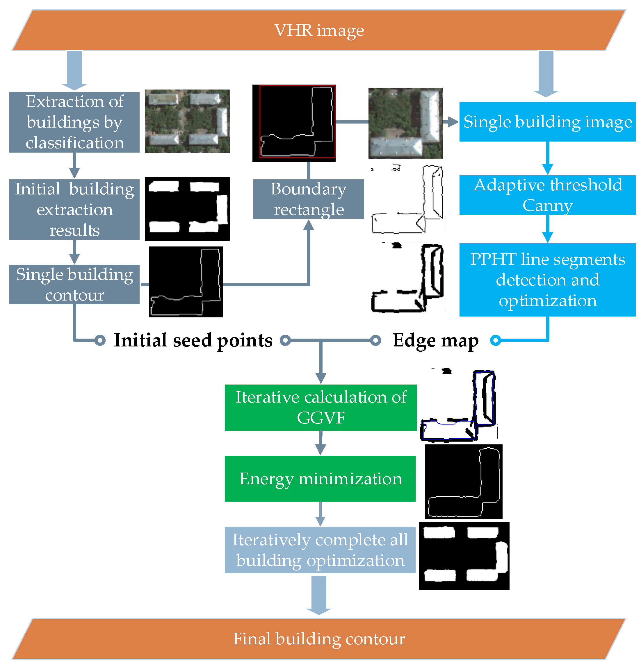
First, the initial building results should be obtained via classification or other methods. To reduce the interference from adjacent object information, each building object image can be clipped according to the boundary rectangle of its initial building from the original image. Afterward, adaptive threshold Canny edge detection is applied to each clipped building image to detect the edge, and PPHT is used to detect the line segments in these edges. These line segments are reconnected as the outer constrained edge, and the initial building contour is used as the inner seed information, both of which are inputted into the GGVF snake model. With this combination, the energy can be rapidly minimized to make the initial contour close to the real outline. The building contour can be optimized by making full use of the line segment information. The flowchart is shown in Figure 1.

Figure 1.
Flowchart of the building contour optimization.
2.1. GGVF Snake Model
By introducing two spatially varying weighting functions into the GVF formulation, Xu and Prince proposed an external force called GGVF [20]. As a generalization of GVF, GGVF was reported to improve contour convergence to LTIs and robustness to noise. GGVF is defined as the equilibrium solution to the following partial differential equation:
where
where t is the iteration time, v(x, y, t) is iteratively calculated from the initial vector field v(x, y, 0), and (x, y, t) denotes the partial derivative of vector field v(x, y, t) with respect to t, and ∇2 is the Laplacian operator. Here, |∇f| is the gradient of the edge map. The weighting function g(·) and h(·) apply to the first (smoothing term) and second terms (data term) in the right-hand side of Equation (1), respectively. The parameter k regulates to some extent the tradeoff between the smoothing and data terms and should be set according to the amount of noise in the image. According to Equations (2) and (3), as k increases, g(|∇f|) and h(|∇f|) in Equation (1) increases and decreases, respectively. That means, as k becomes larger, the GGVF external forces at the indentation boundary are more easily changed. In addition, the larger the tradeoff parameter k, the greater the impact of noise. Therefore, it is necessary to estimate the appropriate maximum k for a given image [23]. The range of k is usually (0.01, 0.2).
2.2. Objected-Oriented GGVF Initial Contour Acquirement
The information surrounding the building in high-resolution remote sensing imagery, such as the adjacent buildings, vegetation, roads, and other objects, are sometimes wrongly recognized, leading to reductions in detection accuracy and efficiency. Therefore, the analysis range of each building is shrunk by clipping each building as a single object according to its boundary rectangle. Specifically, the initial building results can be acquired by using classification or other methods. In this paper, the shadow-shifted classification method proposed in [1] is applied, and the boundary rectangle of each building is obtained and dilated several times to derive its clipping range. The building image object is eventually obtained. Figure 2 shows the schematic diagram of how the building object images are acquired. The initial building contour obtained in this step not only provides the initial building seed information to the GGVF snake model but also can be used to obtain a clipped building image to further detect some line segments as constraint boundary information for optimizing the contour in the GGVF snake model.

Figure 2.
Schematic diagram of obtaining the clipped building object image. (a) Original image; (b) initial extraction results (white) and minimum boundary rectangle (yellow); (c) expanded 3-pixel circumscribed rectangle (purple); and (d) cropped result after 3-pixel expansion.
2.3. GGVF Constraint Edge Map Extraction
Accurate contour constraint segments are important for the GGVF snake model to find the target contour quickly in the optimization process. In this paper, an adaptive threshold Canny edge detection is applied to each building image to detect the edge. Afterward, PPHT is applied to the edge result to extract the line segments. For those cases with missing or wrong line segments in some edges, a hierarchical line segments reconstruction method is proposed to obtain complete contour constraint segments.
2.3.1. Adaptive Canny Edge Detection
The reliable building edges extracted by the Canny detector are vital for line segments using PPHT. First, each clipped image is smoothed via Gaussian convolution. The 2D first derivatives are then used to calculate the gradient magnitude and direction. The first-order derivative of an image f(i, j) at location (i, j) is defined as the following 2D vector [24]:
The absolute gradient magnitude (edge strength) is computed as
The gradient direction (edge orientation) is defined as
Second, a non-maximal suppression process is applied to the gradient magnitude image to remove the local maxima. Only those pixels with an edge strength higher than that of their two adjacent pixels in the gradient direction are identified as edge candidates. To remove false edge segments caused by noise and fine texture, a hysteresis tracking process is further applied with two thresholds in which all candidate edge pixels below the lower threshold are labeled as non-edges, whereas all pixels above the low threshold that can be connected to any pixel above the high threshold through a chain of edge pixels are labeled as edge pixels.
These two thresholds should be suitable for each building to obtain accurate edge detection results. To extract the edge accurately, an adaptive threshold strategy is employed to determine the optimal thresholds for each building. First, the gradient magnitude is normalized to (0, 1). Based on the histogram of the gradient magnitude, the probability sum of one level K can be calculated by consecutively adding the probabilities of each grey level lower than K. PNE denotes the rate of the non-edge point in the whole image.
where K is the rate of non-edge points in the whole edge points, and Im and In are the image height and width, respectively.
Assume that LF_hist is the grey level of the first non-edge point whose probability sum is greater than PNE for the first time, and LT_hist is the grey level total number of the histogram, where LT_hist = 64. The high threshold Thigh represents the ratio between LF_hist and LT_hist and can be determined automatically. The low threshold Tlow is then defined as the ratio of Thigh, where R∈ (0, 1).
As long as R is suitable, Tlow can be determined automatically and adaptively. A series of tests show that R= 0.4 and K = 0.7 are suitable experimental values for most buildings to obtain a reasonable edge. Therefore, the improved automatic threshold strategy is useful for improving the edge accuracy and providing a solid basis for line detection based on PPHT.
2.3.2. Line Segments Detection and Optimization Based on PPHT
The building line segments are extracted to construct the building constraint edge map. PPHT can further extract line segments from those edges obtained by the Canny detector. However, given the complex background of buildings, some line segments extracted by PPHT may not be accurate or enough to construct the constraint edge map. Therefore, based on the line segments extracted by PPHT, a strategy for customizing an effective constraint edge map for different conditions is defined. First, line fitting is applied to connect the adjacent parallel line segments to reduce inference. Second, for the wrongly detected line segments caused by the clipping image, those line segments near the image edge are deleted. The topology relationship between the line segment and the initial building contour is taken into account to delete ineffective segments. Third, a complementary strategy is applied to make the constraint edge map complete by making up for those missing line segments in some directions.
Line Segments Extraction by PPHT
The basis of the Hough transformation is given in Equation (10), where (θ, ρ) and (x, y) represent the Hough transformation and image domains, respectively, whereas δ refers to the Dirac delta function. Each point (x, y) in the original image F(x, y) is transformed into a sinusoid ρ=xcos(θ) − ysin(θ), and H(θ, ρ) represents the total number of sinusoids that intersect at the point (θ, ρ). Therefore, Equation (10) returns the total number of points comprising the line in the original image. By choosing a line-cut threshold T for H(θ, ρ) and by using the inverse Hough transformation, the original image is filtered in order to keep only those lines that contain at least T points [25].
The line segments are extracted by using PPHT, which is improved based on Hough transformation. The main process is to set up an accumulator for each small space in the parameter space and then randomly select the front scenic spot on the image and map this spot to the parameter space to draw a curve. When the intersection of the curves reaches the minimum threshold, the line corresponding to this point is identified. Search for the points on the line in the image, and then connect the qualified points into line segments. If the line segment length meets the minimum length, then record the starting and ending points of the line segment and then repeat the above steps.
Line Segments Fitting
After extracting the line segments, some of them are merged if they are parallel and near enough to reduce similar segments. First, all detected line segments are grouped into set Lset_1= and copied as another set Lset_2=. Each line segment in Lset_1 will be compared with all the segments in Lset_2 to measure the perpendicular distance and the intersection angle between them. Assume that and are the line segments in Lset_1 and Lset_2, respectively, whereas , and and and are the start and end points of and , respectively. Suppose that the perpendicular distance and intersection angle of and r line segments { are small enough to meet the merging requirement. In this case, { will be labeled as the matched segments of . Beginning with , a new average line segment will be generated by connecting the middle points of the start and end points. Afterward, and the corresponding will be removed from Lset_2 and Lset_1. will be compared with the remaining unmatched line segments in {. Continue updating by following the above steps until all matched segments are finished. The final average line segment of will then be added to Lremain until all segments in Lset_1 are finished. The remaining segment group will then be used as the simplified set to replace the original segment group.
| Algorithm 1 Line fitting |
| 1: Input Lset_1 = and Lset_2=. |
| 2: For each in Lset_1 |
| 3: Ltemp= |
| 4: For each in Lset_2 |
| 5: If (Ltemp and are not the same and meet the fitting conditions) |
| 6: Ltemp = Fitting(Ltemp, ) |
| 7: Delete from Lset_1 |
| 8: Delete from Lset_2 |
| 9: End |
| 10: Add Ltemp to Lremain |
| 11: End |
| 12: Output Lremain |
The approximate schematic process of line fitting is shown in Figure 3. Merge_1 shows the fitting of two original PPHT line segments; Merge_2 shows the iterative fitting of the fitting line segment and the original PPHT line segment.

Figure 3.
Line segments from PPHT (blue) merged into one or more collinear line segments (red).
Removing Building Roof Line Segments
Some falsely detected line segments inside the roof region are removed according to their topology relationship with the initial building contour. First, the initial building contours are shrunk via morphology erosion to ensure they are inside the building. Second, the topology relationship between each line segment and the erased building contour is calculated. If one or more endpoints of a line segment are in the erased contour, then the line segment is deleted. Therefore, the remaining line segments around the building contour can be used to accurately construct the building constraint edge map.
Complementing the Incomplete Building Constraint Edge Map
PPHT may not provide complete line segments to construct an effective constraint edge map for GGVF snake model convergence. A reasonable building constraint edge map should contain all edge directions of a building. Therefore, a strategy is developed to complement the missing edge parts. First, by comparing the distance between each PPHT segment and the initial contour for matching, some contours without matched PPHT segments are labeled as the missing edge parts. Second, for these regions, the Shi–Tomasi corner point detection algorithm is applied to the original image to obtain some useful corner points. If some corner points are present in this area, then they are connected to the endpoint in order. Otherwise, the endpoints of the missing parts are connected directly to form a complete constraint edge map. This map is then used in order for the converged GGVF to extract contours accurately. Otherwise, an unclosed or inaccurate edge map will affect the final contour.
2.4. GGVF Force Field Computation
Applying the initial contour and the constraint edge map to the GGVF snake model will help this model rapidly reach convergence to obtain the optimized contour [26]. The initial GGVF vectors v(x, y) = [u(x, y), v(x, y)] are generally normalized with respect to their magnitudes via vector-based normalization. To set up the iterative solution, let the spatial sample intervals be ∆x and ∆y, and let the time step for each iteration be ∆t.
As in [20], the partial differential equation v(x, y, t) specifying GGVF can be implemented by using an explicit finite difference scheme, which is stable if the time step ∆t and the spatial sample intervals ∆x and ∆y satisfy
where is the maximum value of over the range of gradients encountered in the edge map image. An implicit scheme for the numerical implementations of Equation (1) would be unconditionally stable and is therefore not needed in this condition, thereby increasing the speed of the explicit scheme.
An example with intermediate results is shown in Figure 4. The main process includes initial building contour acquisition (Figure 4b), building object clipping (Figure 4c), adaptive threshold Canny edge detection (Figure 4d), PPHT line segment detection (Figure 4e), and GGVF snake iterative calculation to obtain the final result (Figure 4f).

Figure 4.
An example with intermediate results. (a) Original image; (b) initial building results; (c) cropped original image; (d) Canny detection; (e) PPHT segments (black line segments) and GGVF initial contour (blue closed line); and (f) final result.
3. Experiments Results
3.1. Datasets and Experimental Strategy
3.1.1. Dataset Description
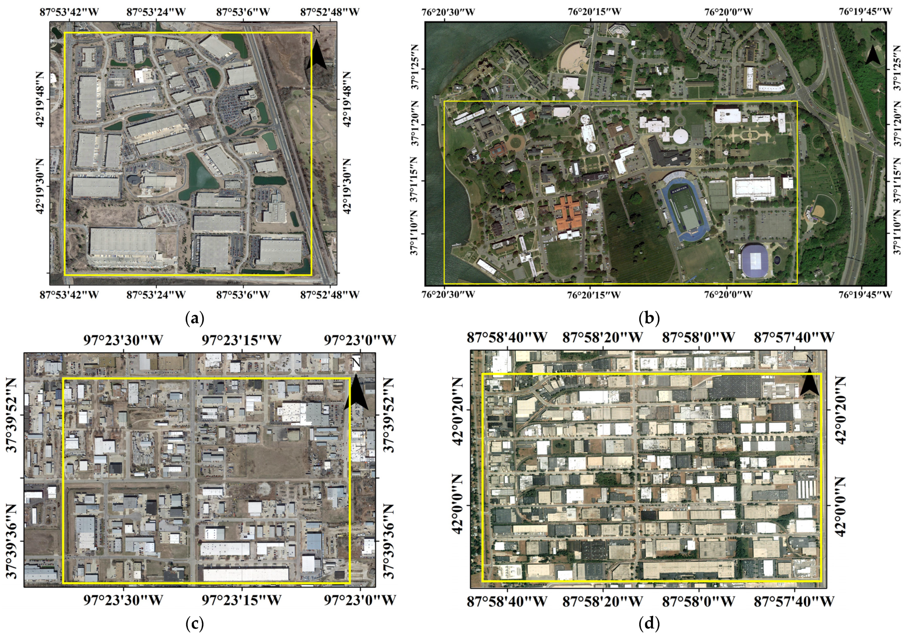
The main experimental areas are in Illinois, Virginia, and Kansas, as shown in Figure 5. The image spatial resolution is 0.4 m. These experimental areas include buildings different in spectra, shape, size, texture, and density. Therefore, these images are adequate to verify the reliability and robustness of the proposed method.
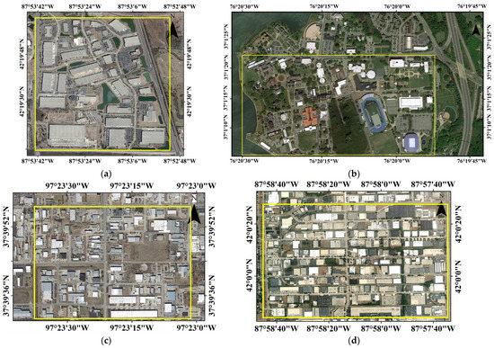
Figure 5.
Origin test image patches. (a) #1 Park City, Chicago; (b) #2 Hampton, Virginia; (c) #3 Wichita, Kansas; and (d) #4 Schomburg, Illinois.
3.1.2. Accuracy Indexes
To objectively evaluate the effectiveness of the proposed method, truth images are extracted by professional staff, and four commonly used accuracy indexes, including completeness (CM), correctness (CR), comprehensive value (F1), and overall accuracy (OA), are used as measures in comparisons with the truth data [27].
where |VTP| is the total number of building pixels that are classified to the building, |VFP| is the total number of non-building pixels that are recognized as buildings, and |VFN| is the total number of building pixels that are labelled as non-buildings.
3.2. Comparison of Experimental Results
3.2.1. Effectiveness Evaluation for Different Initial Results
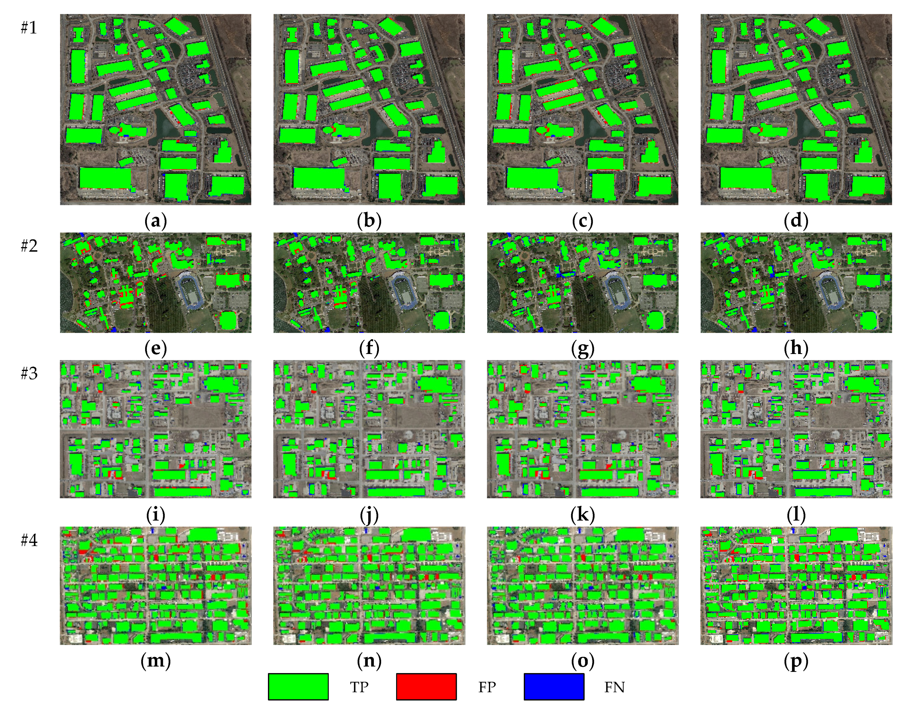
To verify whether the proposed method can be applied to different initial methods, the initial building results extracted by the shift shadow algorithm (SSDA) and the traditional GGVF snake method (TD-GGVF) are optimized by using the proposed method. The SSDA method performs building extraction by classifying an image into the building, bare land, shadow, and vegetation. The building samples are obtained by shifting the shadow region, and the results are verified by using the shadow index. The TD-GGVF obtains the building contour based on the traditional GGVF snake model by manually setting the initial seed points, and then the edge map is obtained based on the original image. These methods based on different principles can provide initial building results that are irregular. Therefore, the proposed method is applied to these two initial results to test its effectiveness. The initial building and optimization results of SSDA and TD-GGVF are shown in Figure 6, and the accuracy comparison results are shown in Table 1.

Figure 6.
Comparison of the optimization results by using the proposed method for different building extraction methods (#1-#4 is shown in Figure 5). (a,e,i,m): building results obtained by the SSDA method; (b,f,j,n): optimization results based on SSDA; (c,g,k,o): building results obtained by the TD-GGVF method; and (d,h,l,p): optimization results based on TD-GGVF.

Table 1.
Comparison of building extraction and optimization results in Figure 6 (the highest values are bold).
From the initial building results, each building extraction method faces the common problem that the building boundaries are irregular. The proposed optimization method can further improve the accuracy of the building boundary. The initial results of the SSDA are shown in the first column in Figure 6, which shows that the proposed method can effectively distinguish buildings from confusing bare land by automatically extracting and verifying samples. However, given the similarity of the spectrum between building and some non-building objects and the occlusion of adjacent vegetation, some false and missing detections are still observed. As reflected in its results, the TD-GGVF method can efficiently extract the building when the building boundary in the original image is clear. Nevertheless, the spectral characteristics of the building and its surroundings are complex. The extraction result becomes inaccurate when the building boundary is not prominent, when the spectrum of the building roof is not uniform, or when a local abnormal spectrum is present on the building roof. The proposed method aims to address these irregularities caused by wrong recognition. As shown in the optimization results, the improvements in the accurate edge extraction and the approximation of the GGVF snake model can refine the building boundary to restore the missing and wrong segmentation parts. The building contour constraint line segments in the proposed method can avoid the spectral interference of the TD-GGVF method. As shown in Table 1, the comprehensive value and overall accuracy of the proposed method are higher than those of the SSDA method. The comprehensive value is improved by 1.41% (SSDA) and 0.98% (TD-GGVF) on average, whereas the overall accuracy is improved by 2.49% (SSDA) and 1.77% (TD-GGVF). The comparison results show that the proposed optimization method can be effectively and automatically used for different building results acquired by classification or the snake model. The optimization is not limited by the building shape and size and can be applied as an effective post-processing tool for improving building regularization and accuracy.
3.2.2. Comparison with Other Contour Optimization Methods
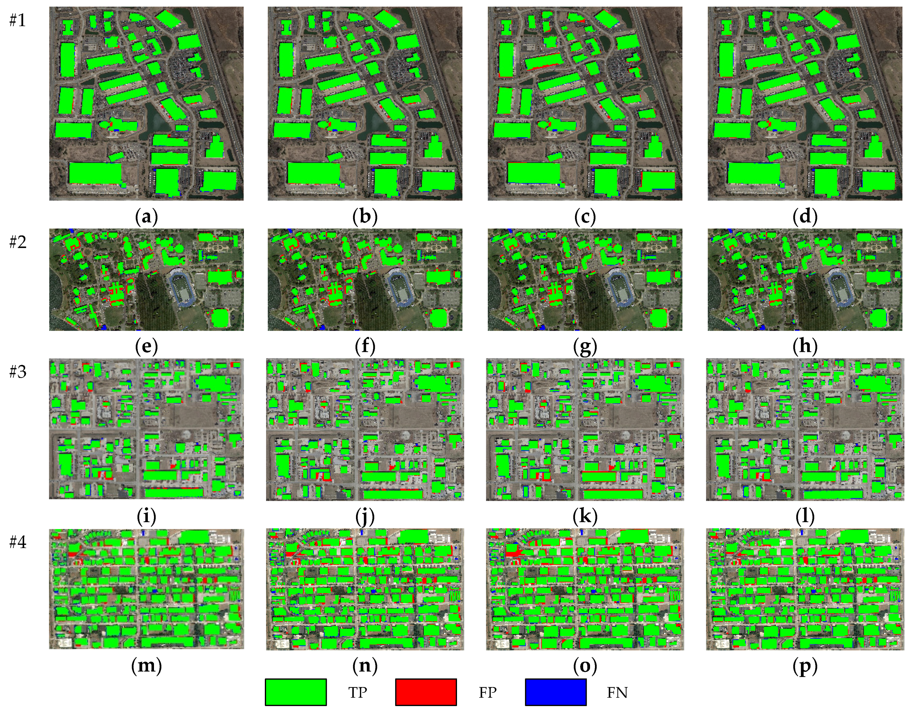
Different contour optimization methods, including the Douglas–Peucker straight-line approximation method (DPSLA) [28], the multi-stars constraint segmentation and regularization method (MCSR), and the proposed method, are applied to the same initial building results (first column of Figure 7) for comparison. DPSLA aims to find a fitting polygon of building results by removing those contour points near the line segments connected by the front and back points of these contour points. MCSR optimizes the building edge by grouping, line fitting, and line rotation after corner extraction. The results of the representative patches in each test image are visualized in Figure 7, and the precision is shown in Table 2.
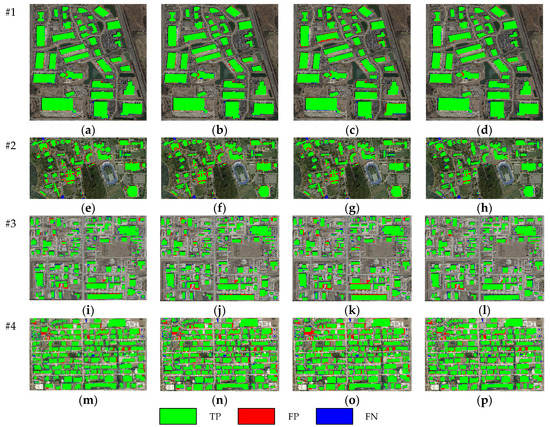
Figure 7.
Comparison of different optimization methods (#1-#4 is shown in Figure 5). (a,e,i,m): initial building results; (b,f,j,n): DPSLA method; (c,g,k,o): MCSR method; (d,h,l,p): proposed method.

Table 2.
Comparison of image optimization results obtained by different optimization methods in Figure 7 (the highest values are bold).
An analysis of the comparison results in Figure 7 reveals that the proposed method is more powerful and feasible than other methods, improving buildings of different shapes. DPSLA is sufficient that some small broken line segments can be approximated into a straight line, and the building outline is regularized to a certain extent. However, DPSLA is greatly affected by the initial building results and is unable to correct the wrong and missing parts in the initial results. Moreover, MCSR in [11] is useful in optimizing rectangular building contours and helps regularize the initial results. Nevertheless, for complex buildings with arcs or non-right angles, MCSR improperly deals with these edges, thereby leading to misclassification in these areas. By contrast, by combining the profile spectrum and texture characteristics of buildings, the proposed method makes full use of the active contour model to accurately approximate the real contours. Therefore, this method is not affected by the initial building results and building shapes. Despite some wrong detection or missing parts in initial buildings, the proposed method correctly self-adapts through the optimization process. The data analysis results in Table 2 show that compared with DPSLA and MCSR, the proposed method has a comprehensive value that is 1.63% (DPSLA) and 2.16% (MCSR) higher on average and an overall accuracy that is 2.86% (DPSLA) and 3.84% (MCSR) higher on average. Therefore, the optimization capability of the proposed method is more powerful and self-adjustable than that of other methods to approach the real building shape.
4. Discussion
4.1. The Positive Effect of Improved Automatic Canny Detector
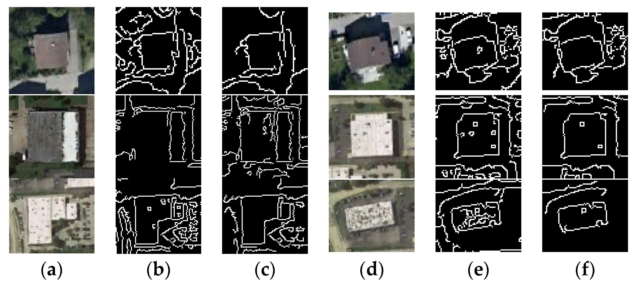
The Canny detector automatic threshold is vital in determining effective edge segments that can be used in the next PPHT. To illustrate the advantages of the adaptive threshold method in Canny detection, a comparison test using a different threshold strategy is performed, as shown in Figure 8. The results in Figure 8b,e are obtained from the whole image by using the global unified threshold method, whereas those in Figure 8c,f are obtained by using the improved automatic threshold strategy. Each building is detected by its corresponding customized threshold. Given the differences in the characteristics of each building, the global threshold cannot be suitable for each building, thereby creating deviations in the edge detection results. In comparison, the designed strategy in the Canny detector can obtain different thresholds for each building without manual help. Therefore, the threshold facilitates the accurate detection of edges.
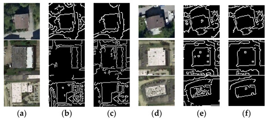
Figure 8.
Comparison of the adaptive and manual global threshold Canny edge detection results. (a,d) present the results for the original image; (b,e) present the results of the Canny edge detection with the manual global threshold; and (c,f) present the results of the Canny edge detection with the adaptive threshold.
4.2. The Positive Effect of Constructing Constraint Line Segments Based on PPHT
Effective line segments serve as vital bases for constructing a complete constraint contour for the GGVF snake model. To verify the effectiveness of these constraint line segments on buildings with different shapes, the results are compared with the original PPHT results, as shown in Figure 9. The straight-line segment detected by PPHT is shown in Figure 9c. Some line segments are overlooked or redundant in the detection (denoted by the red closed line), thereby resulting in missing or inaccurate constraint line segments on one side of the detected building contour. Results of the improved constraint line segments are shown in Figure 9d. Compared with the PPHT line segments, the missing contour line segments can be supplemented more accurately, and some inside line segments are removed. Therefore, the constraint line segments that conform to the building contour can be obtained and used to construct an edge map.

Figure 9.
Comparison results of the building contour constraint line segment. (a) Original images; (b) Canny edge detection; (c) PPHT line segments; and (d) optimized contour constraint line segment.
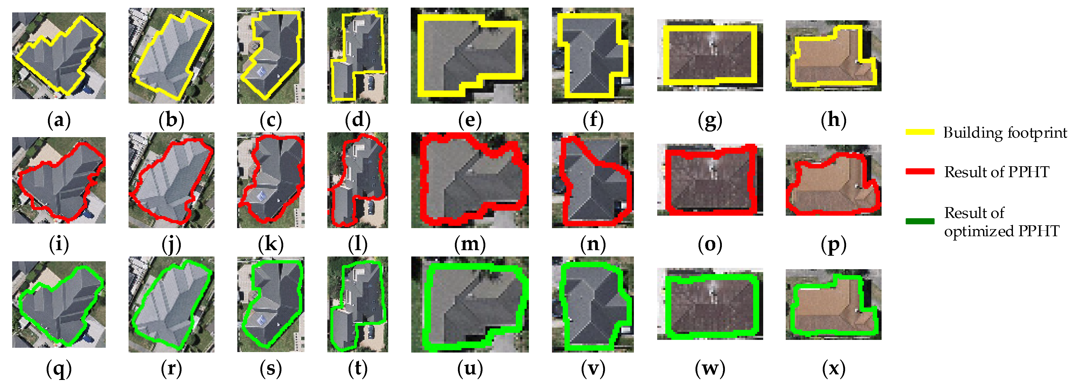
Eight individual building images are randomly selected and compared with the results without the improved PPHT constraint line segments. In Figure 10, the first row shows the truth building contour, the second row presents the results based on the original PPHT line segments, and the third row presents the results based on the improved PPHT line segments. The PPHT optimization results are smooth on the boundary and close to the true shape of the building. Given that the optimization on PPHT can provide more accurate constraint line segments for constructing an edge map, this approach can be used to compute a final contour that is near the original boundary of the building. The comparison results verify the effectiveness and reliability of PPHT optimization.
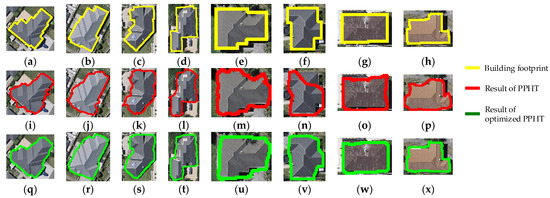
Figure 10.
(a–h): building contour footprints; (i–p): building extraction results obtained by using the original PPHT line segments; and (q–x): building extraction results obtained by using the optimized PPHT line segments.
4.3. Overall Comparison Analysis
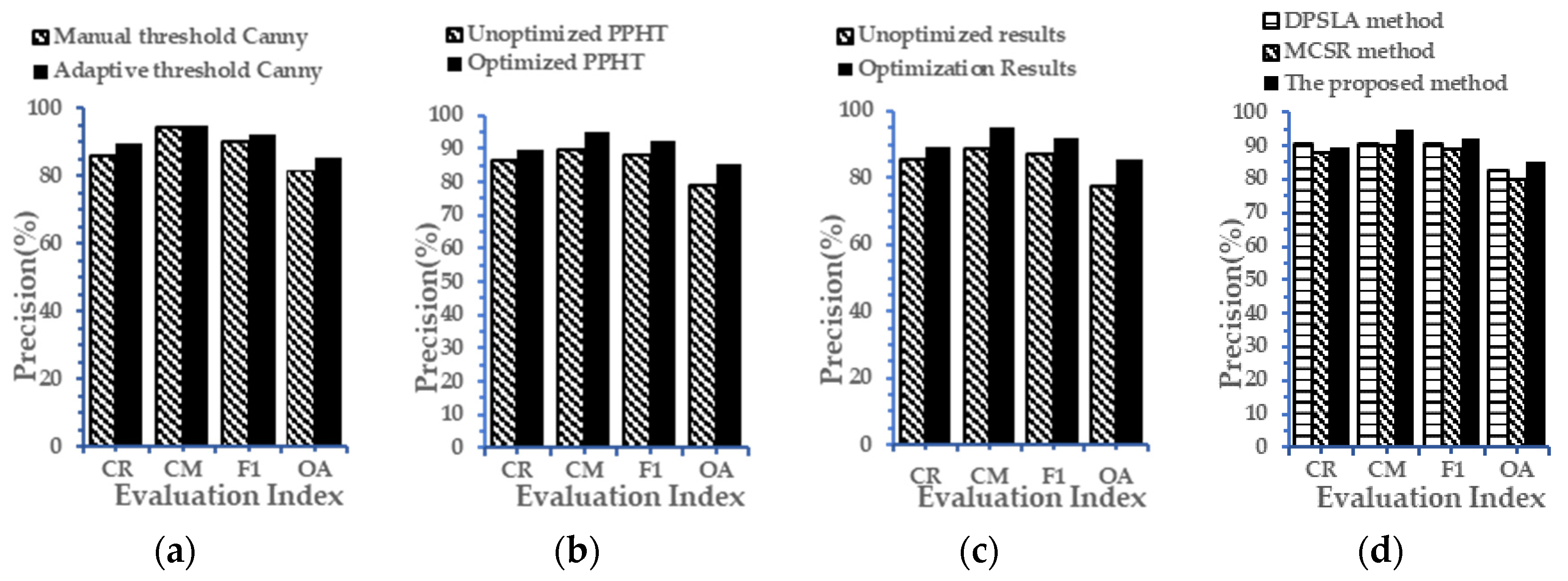
To analyze the contribution of each improvement in the whole optimization process and compare the proposed method with other contour methods in terms of quantity, over 200 buildings are randomly selected from the WHU building dataset [29], and their contours are optimized by using different strategies in Canny detection, constraint line segments, and other optimization methods. The accuracy results are shown in Figure 11. Figure 11a shows the accuracy difference between using the adaptive and manual thresholds in the Canny detection step. The improvement in Canny detection accuracy can increase the F1 and overall precision by 2.35% and 3.83%, respectively. Figure 11b shows the accuracy difference between using the optimized and original PPHT constraint line segments. The improvement in constraint line segments enhances the F1 and overall precision by 3.92% and 6.47%, respectively. Figure 11c compares the proposed method that uses both the adaptive threshold Canny and PPHT segment optimization with the original method that lacks these two improvements. Combining the self-adaptive Canny detector with the optimized PPHT segments improves the F1 and overall precision by 4.94% and 8.13%, respectively. Therefore, the proposed method is proven effective. Figure 11d compares the proposed method with two other methods for optimizing the building contour, namely, DPSLA and MCSR, and shows that the proposed method obtains the higher F1 and overall precision. In sum, the proposed method optimizes the GGVF snake model by introducing the Canny detector and PPHT line segments, which are useful in constructing a suitable constraint edge map for each building and improving building accuracy.
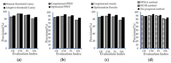
Figure 11.
Accuracy comparison. (a) Adaptive threshold vs. manual global threshold; (b) optimized vs. unoptimized PPHT; (c) optimization proposed by this method vs. unoptimization proposed by this method; and (d) proposed method vs. other optimization methods.
4.4. Comparisons of Time Complexity
In this part, we discuss the main time complexity [30] of the proposed and compared methods in the experiments. In the proposed method, the first step is to gain the building contours [31] and sub-images. The second step is to detect Canny [32] edge with the adaptive threshold. The third is to obtain the building constraint edge map. The last step is to gain the final building contour through GGVF [33]. The main time complexity of each step is shown in Table 3. As we can see, the main time cost is in the fourth step, and the total time complexity of the proposed method is O(WlHl + + WsHs + + ). As we have Wl Ws and Hl Hs, the time cost can be simplified as O(WlHl + + WsHs + + ) O(WlHl + + + ). The complexity of DPSLA [28] depends mainly on the number of building contour points. Thus, in general, the complexity of the DPSLA is O(WlHl + ). As for the main time complexity of MCSR [11], it depends on the number of building contour points and the number of corner points detected. For MSCR, the time complexity is O(WlHl + ). The method proposed in this paper has higher time complexity than that of the compared methods. This is because the method proposed in this paper has more steps and considers them more comprehensively.

Table 3.
The time complexity of the compared methods 1.
5. Conclusions
Building extraction results often show irregular building contours because of inaccurate recognition, and most of the extant optimization methods are limited only to rectangular non-complex buildings. To devise a contour optimization method for complex buildings, an object-oriented strategy combined with the GGVF snake model is proposed in this paper. First, based on the initial building extraction results, each building object is clipped from images to reduce the impact of the adjacent non-building objects. Second, a building boundary shrunk based on the initial result is used as the initial contour of the GGVF and is automatically obtained. Third, a Canny edge detection with adaptive threshold and the optimized PPHT line segments are designed to obtain a highly accurate constraint edge map. Fourth, after inputting the accurate and automatic initial contour and edge map into the GGVF snake model, the building contour is calculated feasibly and self-adaptively. The proposed method is not limited by the complexity of buildings. Experimental verifications confirm that the proposed method not only optimizes the building outline but also improves the final accuracy of building extraction to a certain extent. This method can also optimize the contour similar to the real building shape. The proposed method may be applied as a post-process method for building extraction to improve the regularity and accuracy of buildings.
Author Contributions
J.C. conceived and conducted the experiments. Y.Y. performed the data analysis. N.W. and X.G. revised the manuscript. J.C. wrote the article. All authors have read and agreed to the published version of the manuscript.
Funding
This research is supported by Open Fund of Key Laboratory of National Geographic Census and Monitoring, Ministry of Natural Resources Open Fund (No. 2020NGCM07); Open Fund of National Engineering Laboratory for Digital Construction and Evaluation Technology of Urban Rail Transit(No.2021ZH02); Open Fund of Hunan Provincial Key Laboratory of Geo-Information Engineering in Surveying, Mapping and Remote Sensing, Hunan University of Science and Technology (No.E22133); Open Fund of Beijing Key Laboratory of Urban Spatial Information Engineering (No.20210205); the Open Research Fund of Key Laboratory of Earth Observation of Hainan Province (No.2020LDE001); the National Natural Science Foundation of China (No. 41872129).
Acknowledgments
We would like to thank the anonymous reviewers for their constructive and valuable suggestions on the earlier drafts of this manuscript.
Conflicts of Interest
The authors declare no conflict of interest.
References
- Gao, X.; Wang, M.; Yang, Y.; Li, G. Building Extraction From RGB VHR Images Using Shifted Shadow Algorithm. IEEE Access 2018, 6, 22034–22045. [Google Scholar] [CrossRef]
- Wang, Z.; Du, B.; Zhang, L.; Zhang, L.; Jia, X. A Novel Semisupervised Active-Learning Algorithm for Hyperspectral Image Classification. IEEE Trans. Geosci. Remote Sens. 2017, 55, 3071–3083. [Google Scholar] [CrossRef]
- Chen, M.; Wu, J.; Liu, L.; Zhao, W.; Tian, F.; Shen, Q.; Zhao, B.; Du, R. DR-Net: An Improved Network for Building Extraction from High Resolution Remote Sensing Image. Remote Sens. 2021, 13, 294. [Google Scholar] [CrossRef]
- Wang, Z.; Du, B.; Guo, Y. Domain Adaptation With Neural Embedding Matching. IEEE Trans. Neural Netw. Learn. Syst. 2020, 31, 2387–2397. [Google Scholar] [CrossRef]
- Dey, E.K.; Awrangjeb, M.; Stantic, B. Outlier Detection and Robust Plane Fitting for Building Roof Extraction from LiDAR Data. Int. J. Remote Sens. 2020, 41, 6325–6354. [Google Scholar] [CrossRef]
- Dong, Y.; Liang, T.; Zhang, Y.; Du, B. Spectral–Spatial Weighted Kernel Manifold Embedded Distribution Alignment for Remote Sensing Image Classification. IEEE Trans. Cybern. 2021, 51, 3185–3197. [Google Scholar] [CrossRef] [PubMed]
- Lee, D.S.; Shan, J.; Bethel, J.S. Class-Guided Building Extraction from Ikonos Imagery. Photogramm. Eng. Remote Sens. 2003, 69, 143–150. [Google Scholar] [CrossRef]
- Albers, B.; Kada, M.; Wichmann, A. Automatic Extraction and Regularization of Building Outlines from Airborne Lidar Point Clouds. Int. Arch. Photogramm. Remote Sens. Spatial Inf. Sci. 2016, XLI-B3, 555–560. [Google Scholar] [CrossRef]
- Sampath, A.; Shan, J. Building Boundary Tracing and Regularization from Airborne Lidar Point Clouds. Photogramm. Eng. Remote Sens. 2007, 73, 805–812. [Google Scholar] [CrossRef]
- Partovi, T.; Bahmanyar, R.; Kraus, T.; Reinartz, P. Building Outline Extraction Using a Heuristic Approach Based on Generalization of Line Segments. IEEE J. Sel. Top. Appl. Earth Obs. Remote Sens. 2017, 10, 933–947. [Google Scholar] [CrossRef]
- Ding, Y.; Feng, F.; Li, J.; Hu, Y.; Cui, W. Right-Angle Buildings Extraction from High-Resolution Aerial Image Based on Multi-stars Constraint Segmentation and Regularization. Acta Geod. Cartogr. Sin. 2018, 47, 1630–1639. [Google Scholar] [CrossRef]
- Kwak, E.; Habib, A. Automatic Representation and Reconstruction of DBM from LiDAR Data Using Recursive Minimum Bounding Rectangle. ISPRS J. Photogramm. Remote Sens. 2014, 93, 171–191. [Google Scholar] [CrossRef]
- Feng, M.; Zhang, T.; Li, S.; Jin, G.; Xia, Y. An Improved Minimum Bounding Rectangle Algorithm for Regularized Building Boundary Extraction from Aerial LiDAR Point Clouds with Partial Occlusions. Int. J. Remote Sens. 2020, 41, 300–319. [Google Scholar] [CrossRef]
- Chang, J.; Wang, S.; Yang, Y.; Gao, X. Hierarchical Optimization Method of Building Contour in High-Resolution Remote Sensing Images. Chin. J. Las. 2020, 47, 249–262. [Google Scholar] [CrossRef]
- Kass, M.; Witkin, A.; Terzopoulos, D. Snakes: Active Contour Models. Int. J. Comput. Vis. 1988, 1, 321–331. [Google Scholar] [CrossRef]
- Peng, J.; Liu, Y.C. Model and Context-driven Building Extraction in Dense Urban Aerial Images. Int. J. Remote Sens. 2005, 26, 1289–1307. [Google Scholar] [CrossRef]
- Ahmadi, S.; Zoej, M.J.V.; Ebadi, H.; Moghaddam, H.A.; Mohammadzadeh, A. Automatic Urban Building Boundary Extraction from High Resolution Aerial Images Using an Innovative Model of Active Contours. Int. J. Appl. Earth Obs. Geoinf. 2010, 12, 150–157. [Google Scholar] [CrossRef]
- Liasis, G.; Stavrou, S. Building Extraction in Satellite Images Using Active Contours and Colour Features. Int. J. Remote Sens. 2016, 37, 1127–1153. [Google Scholar] [CrossRef]
- Akbulut, Z.; Özdemir, S.; Acar, H.; Karsli, F. Automatic Building Extraction from Image and LiDAR Data with Active Contour Segmentation. J. Indian Soc. Remote Sens. 2018, 46, 2057–2068. [Google Scholar] [CrossRef]
- Xu, C.; Prince, J.L. Generalized Gradient Vector Flow External Forces for Active Contours. Signal Process. 1998, 71, 131–139. [Google Scholar] [CrossRef]
- Matas, J.; Galambos, C.; Kittler, J. Robust Detection of Lines Using the Progressive Probabilistic Hough Transform. Comput. Vis. Image Underst. 2000, 78, 119–137. [Google Scholar] [CrossRef]
- Xu, C.; Prince, J.L. Snakes, Shapes, and Gradient Vector Flow. IEEE Trans. Image Process. 1998, 7, 359–369. [Google Scholar] [CrossRef] [PubMed]
- Qin, L.; Zhu, C.; Zhao, Y.; Bai, H.; Tian, H. Generalized Gradient Vector Flow for Snakes: New Observations, Analysis, and Improvement. IEEE Trans. Circuits Syst. Video Technol. 2013, 23, 883–897. [Google Scholar] [CrossRef]
- Liu, H.; Jezek, K.C. Automated Extraction of Coastline from Satellite Imagery by Integrating Canny Edge Detection and Locally Adaptive Thresholding Methods. Int. J. Remote Sens. 2004, 25, 937–958. [Google Scholar] [CrossRef]
- Turker, M.; Koc-San, D. Building Extraction from High-Resolution Optical Spaceborne Images Using the Integration of Support Vector Machine (SVM) Classification, Hough Transformation and Perceptual Grouping. Int. J. Appl. Earth Obs. Geoinf. 2015, 34, 58–69. [Google Scholar] [CrossRef]
- Anand, A.; Tripathy, S.S.; Kumar, R.S. An Improved Edge Detection Using Morphological Laplacian of Gaussian Operator. In Proceedings of the 2015 2nd International Conference on Signal Processing and Integrated Networks (SPIN), Noida, India, 19–20 February 2015; IEEE: Noida, India, 2015; pp. 532–536. [Google Scholar]
- Wang, J.; Yang, X.; Qin, X.; Ye, X.; Qin, Q. An Efficient Approach for Automatic Rectangular Building Extraction From Very High Resolution Optical Satellite Imagery. IEEE Geosci. Remote Sens. Lett. 2015, 12, 487–491. [Google Scholar] [CrossRef]
- Douglas, D.H.; Peucker, T.K. Algorithms for the Reduction of the Number of Points Required to Represent a Digitized Line or Its Caricature. Cartogr. Int. J. Geogr. Inf. Geovis. 1973, 10, 112–122. [Google Scholar] [CrossRef]
- Ji, S.; Wei, S.; Lu, M. Fully Convolutional Networks for Multisource Building Extraction From an Open Aerial and Satellite Imagery Data Set. IEEE Trans. Geosci. Remote Sens. 2019, 57, 574–586. [Google Scholar] [CrossRef]
- Wang, Z.; Du, B.; Tu, W.; Zhang, L.; Tao, D. Incorporating Distribution Matching into Uncertainty for Multiple Kernel Active Learning. IEEE Trans. Knowl. Data Eng. 2021, 33, 128–142. [Google Scholar] [CrossRef]
- Suzuki, S.; Abe, K. Topological Structural Analysis of Digitized Binary Images by Border Following. Comput. Vis. Graph. Image Process. 1985, 30, 32–46. [Google Scholar] [CrossRef]
- Kalbasi, M.; Nikmehr, H. Noise-Robust, Reconfigurable Canny Edge Detection and Its Hardware Realization. IEEE Access 2020, 8, 39934–39945. [Google Scholar] [CrossRef]
- Li, B.; Acton, S.T. Active Contour External Force Using Vector Field Convolution for Image Segmentation. IEEE Trans. Image Process. 2007, 16, 2096–2106. [Google Scholar] [CrossRef] [PubMed]
Publisher’s Note: MDPI stays neutral with regard to jurisdictional claims in published maps and institutional affiliations. |
© 2021 by the authors. Licensee MDPI, Basel, Switzerland. This article is an open access article distributed under the terms and conditions of the Creative Commons Attribution (CC BY) license (https://creativecommons.org/licenses/by/4.0/).

