The Extraction of Street Curbs from Mobile Laser Scanning Data in Urban Areas

Abstract

The demand for mobile laser scanning in urban areas has grown in recent years. Mobile-based light detection and ranging (LiDAR) technology can be used to collect high-precision digital information on city roads and building façades. However, due to the small size of curbs, the information that can be used for curb detection is limited. Moreover, occlusion may cause the extraction method unable to correctly capture the curb area. This paper presents the development of an algorithm for extracting street curbs from mobile-based LiDAR point cloud data to support city managers in street deformation monitoring and urban street reconstruction. The proposed method extracts curbs in three complex scenarios: vegetation covering the curbs, curved street curbs, and occlusion curbs by vehicles, pedestrians. This paper combined both spatial information and geometric information, using the spatial attributes of the road boundary. It can adapt to different heights and different road boundary structures. Analyses of real study sites show the rationality and applicability of this method for obtaining accurate results in curb-based street extraction from mobile-based LiDAR data. The overall performance of road curb extraction is fully discussed, and the results are shown to be promising. Both the completeness and correctness of the extracted left and right road edges are greater than 98%.

1. Introduction

Mobile-based light detection and ranging (LiDAR) systems are increasingly considered useful tools for city management. A mobile-based LiDAR system includes a laser scanner, an inertial measurement unit (IMU), and global navigation satellite system (GNSS) capabilities. Mobile-based LiDAR can be used to collect 3D spatial information in order to build information models for purposes such as 3D city modeling [1], road and street planning and maintenance, virtual geographic environment modeling, and location-based services. Mobile-based LiDAR is currently the most popular system for acquiring accurate 3D data that can be utilized in geographic modeling.

Road information is an important component of basic geographic information [2,3], and highly accurate and precise road information plays an important role in urban planning, traffic control, and emergency response [4,5]. However, at present, spatial vector road data are mainly recorded as two-dimensional (2D) information rather than as three-dimensional (3D) road data, and such 2D data are unable to serve the needs of 3D navigation and intelligent city modeling. In recent years, with vehicles as platforms, integrated Global Positioning System (GPS) systems, inertial navigation systems (INSs), laser scanners, charge-coupled device (CCD) cameras, and other sensors have undergone rapid development. Based on sensor synchronization control, geometric data on city streets and building façades as well as texture information can be collected using a mobile-based LiDAR system. Such systems also provide a new means of rapidly assessing road information and generating a 3D road environment [6].

As part of a city street scene, streets and street curbs can be abstracted to support city managers in urban street reconstruction and environmental management. In particular, the extraction of street curbs has been a popular topic for urban managers for some time now [7]. In most urban road systems, the road boundaries are defined by the locations of the curbs on both sides [8]. A curb is a line of stone or concrete forming an edge between a pavement and a roadway. Curbs are important features for the separation of lanes and restricted areas; thus, curb extraction is very important for ensuring the safety of autonomous driving [9]. Vehicles should remain on the road between the left and right curbs, while most pedestrians will be on the sidewalk. By providing information about the outer boundaries of the roadway, methods of detecting and locating curbs can prevent vehicles from driving onto the sidewalk [10]. Moreover, curb information can also be used to determine the types and exact locations of road junctions, which are significant for local path planning [11]. In addition, due to the occlusion caused by trees and high-rise buildings in urban environments, curbs have recently become a common basis for location estimation [12].

Beyond road system applications, edge extraction can also be applied for the monitoring of train tracks. For railway managers, an important safety management concern is to be able to detect grass lying above the train tracks so that it can be removed later. Therefore, methods of detecting objects obstructing the boundaries of either streets or tracks can support environmental safety monitoring for railway managers as well as autonomous driving and city managers.

There are two general kinds of vision-based methods for extracting curbs: appearance-based methods and geometry-based methods [13]. Various types of appearance features (such as color, reflection intensity, and texture) have been widely used in road detection, while geometry-based methods usually use road boundary or road surface models to describe the geometric features of road areas. Most of these methods are susceptible to shadow effects, and low-level cues adopted for the geometric models. Simple geometric models cannot be used to accurately extract road areas or boundaries.

A large number of researchers willing to use appearance-based methods to extract street curbs. Brenner et al. [14] utilized a mobile-based LiDAR system and collected point cloud data with StreetMapper. Later, Kaartinen et al. [15] used a permanent test field to test the performance of research-based MLS systems, and the results showed that the accuracy of the point cloud data depends on the accuracy of sensors. Graham [16] provided an overview of the most recent MLS technology, and the same article also offered promising approaches for street object extraction in the form of automated algorithms for MLS data processing. Graham’s results showed that it could be difficult to capture the complete point clouds and all different types of objects. However, the author seems to have collected the simplest data set—a data set without barriers. Therefore, the robustness of the method is not established. Li et al. [17] utilized the intensity of the reflectance of objects to recognize different road markings. Guan et al. [18] used image data to extract road markings as a basis for quality control or quality assessment in city management. Yang et al. [19] segmented a geometric reference feature image using intensity and elevation difference information and defined solid-edge lines as road outlines and broken lines as lane lines. Finally, the roadmap was estimated by integrating semantic knowledge, such as shape and size. These authors used reflection intensity or brightness information to extract road edged. Notably, intensity data are highly dependent on the angle of incidence of the laser pulse, the range of the scanner to the object, and the material properties of the road surface.

In addition, some authors have used geometric methods to extract street curbs. Liu et al. [20] presented an algorithm for edge detection with a two-dimensional laser rangefinder. The slope, height difference, and height variance features were used to extract the candidate edge points in DEM, and ID GPR was used to represent the straight edge and curve edge. Hervieu et al. [21] introduced a novel prediction/estimation process that used two RIEGLs to identify curbs and ramps. The angle between the normal direction of a point and the ground was considered an important feature to classify a point as a candidate curb. Zhang et al. [22] used a 2D LiDAR sensor and projected point cloud data onto the plane perpendicular to the ground, followed by curb extraction based on the elevation feature of the curb. Jaakkola et al. [23] proposed automatic methods for classifying the road marking and curbstone points and modeling the road surface as a triangulated irregular network. Nonetheless, this method had not been further verified in sheltered areas or curved streets. Rodríguez-Cuenca et al. [24], based on a rasterization and segmentation approach for curb detection, this method was able to detect upper and lower curb edges. However, it was difficult to deal with occluded curbs in curved sections and with boundaries without 3D shapes. Then, Rodríguez-Cuenca et al. [25] proceeded to propose a segmentation algorithm based on morphological operations to determine the location of street boundaries.

Many different methods of curb detection have been tested, but there is still no reliable curb detection system on the automotive market. In essence, the detection of curbs in general road scenes is challenging for the following reasons: (1) The heights of curbs can vary greatly, not only in different scenes but also in the same image or scanner frame. (2) Due to the small size of curbs, the information that can be used for curb detection is limited. (3) Occlusion, which is very common in road scenes, may cause a method based on line fitting to be unable to correctly capture the curb area [26].

Various types of appearance features are generally based on the reflection intensity or texture information to extract the road edge, while geometry-based methods usually use the road boundary or road plane model to describe the geometric features of the road area. Generally, most of these methods are affected by the degradation caused by shadows, and the algorithms used in simple geometric models can not accurately depict the road area or boundary. This article mainly extracts the curbs of complex three-dimensional urban scenes. The three complex scenes include vegetation covering the curbs, curved curbs, and occlusion curbs. The authors found that on some highways, there is grass next to the motorway, and no special sidewalk in reality. It makes walking inconvenient due to the bushes and tall weeds growing next to or over the curb. Thus, the author believes that the other side of the traffic lane in the roadside (pedestrian zone) information would be introduced into the three-dimensional model of the city, and certain algorithms can be used to identify whether it is grass or wasteland suitable for people to walk above the pedestrian zone. Grassland and weeds are very important factors that affect people’s walking. Therefore, it is necessary to determine the type of ground cover above and near the curb.

The rest of the paper is organized as follows. In Section 2, we present our approach and the workflow. In Section 3, we explain the individual steps involved and the technical basis of curb extraction in three complex environments. In Section 4, we introduce the case study area and the data acquisition. Then we discuss our visual results and quantitative evaluation in Section 5. We conclude in the sixth section where we point to open questions and unresolved problems.

2. System Overview

In this paper, a 3D laser scanner data is used for road edge detection. Different from previous methods, the algorithm proposed in this paper attempts to improve the robustness of the results by combining both spatial information and geometric information.

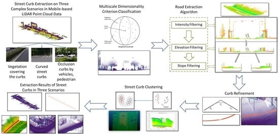
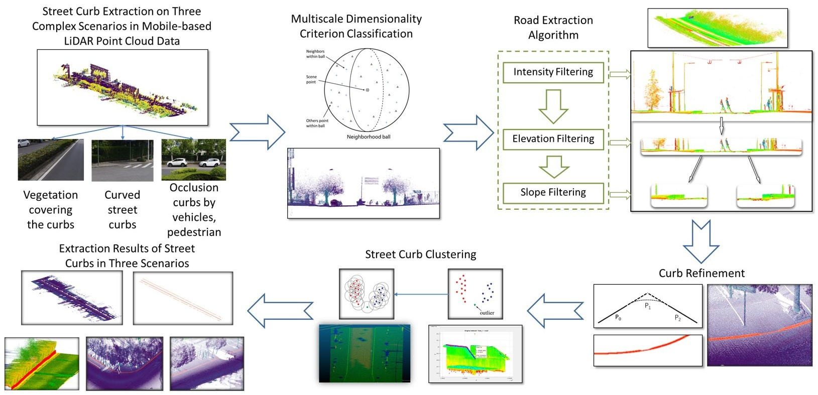
In this study, we use the 3D point cloud data obtained by the Robin scanner, which can generate accurate point clouds. Robin uses the RIEGL VUX-1HA scanner and the specific parameters of the Robin scanner are described in data acquisition in Section 4. This paper introduced a novel method for extracting street curbs. Multiscale dimensionality criterion classification is used to classify and extract vegetation point cloud data. Then, using the characteristics of elevation, echo intensity, and slope change, the street curbs can be detected from the accurate LiDAR point cloud. We use the Otsu threshold method [27] to determine the intensity value, establish the DEM model to determine the elevation slope, and identify the curb according to the spatial slope information of the curb. Then, the quadratic Bézier curve spline was applied to fit the road boundary line segment. Finally, using the Radial Bounded Nearest Neighbor Graph (RBNN) clustering algorithm, the extracted boundary points are clustered to remove some pseudo boundary points. The full procedure of proposed method shows in Figure 1.

Our approach has several advantages. First, different from existing methods that rely only on elevation differently or edge detection, our method considers different shapes and different environments of curbs. It can automatically detect and locate the curb without knowing its shape, length, or distance from the car. In addition, it can deal with special situations such as road curbs blocked by driving vehicles and pedestrians, the curvature of roads, and so on. Finally, it does not need much prior information. We tested our method with a mobile laser scanner in the urban area of Shanghai. The results verify the robustness and effectiveness of our method.

3. Method

This paper presents the development of an algorithm for the extraction of road curbs in an urban area. The procedure consists of three steps: multiscale dimensionality classification to classify and extract vegetation from point cloud data; the use of the characteristics of elevation, echo intensity, and slope change to detect street curbs from the LiDAR point cloud; and the use of the KNN clustering algorithm to cluster the extracted boundary points and remove some pseudo boundary points.

3.1. Classification

Although street curbs extraction algorithms using LiDAR often produce good results with better accuracy and integrity, due to the lack of spectral information, vegetation needs to be removed before filtering classification. Thus, before extracting curb information from the data collected during the mobile laser scanner acquisition process, we need to remove the data on objects that are not of interest to us, such as grass and trees. In this stage, we need to classify all of the data and remove the extraneous data through classification. To this end, vegetation information will be classified first. In this paper, we use a multiscale dimensionality criterion to classify 3D LiDAR data from different kinds of natural scenes.

In the general urban environment, the main types of features are buildings, vegetation, grassland, road information, road signs, cars, and humans. In the proposed algorithm for road edge extraction, all external information that can interfere with edge extraction in an urban environment is taken into account, and different solutions are proposed for different situations. At the stage of multi-scale dimensionality criterion classification, vegetation and grassland point clouds should be identified. The mirror effect (reflection) of 3D scanning water bodies can be an important source of noise (possibly with a high elevation) in the point cloud data. However, it would be further segmented in the process of slope filtering, the reason for that is the elevation change of the water surface is very small. Buildings are identified mainly in the process of intensity filtering.

The main purpose of vegetation classification is to restrain the branches of street trees or the point cloud data of areas of lawn on both sides of the sidewalk, which may affect the extraction of road edges. In the process of vegetation classification, we only need to identify the dense branches of roadside trees and the point cloud of the lawn. Because the accuracy and precision of multi-scale dimensionality criterion classification are very high for vegetation extraction, there are few false extraction cases. Even if some vegetation is not recognized in the dense vegetation point cloud data, the discrete point cloud will not affect the road edge extraction, and the discrete point cloud will be recognized in the subsequent KNN algorithm.

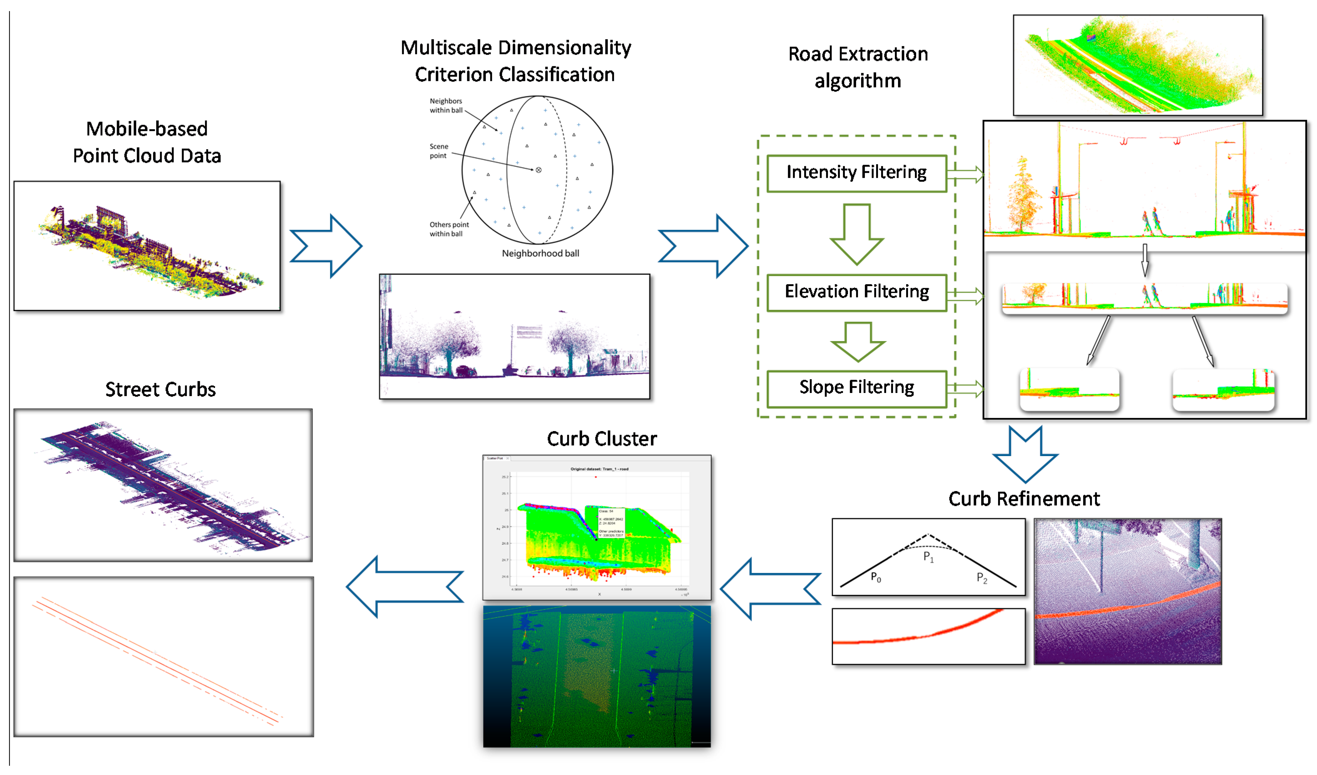
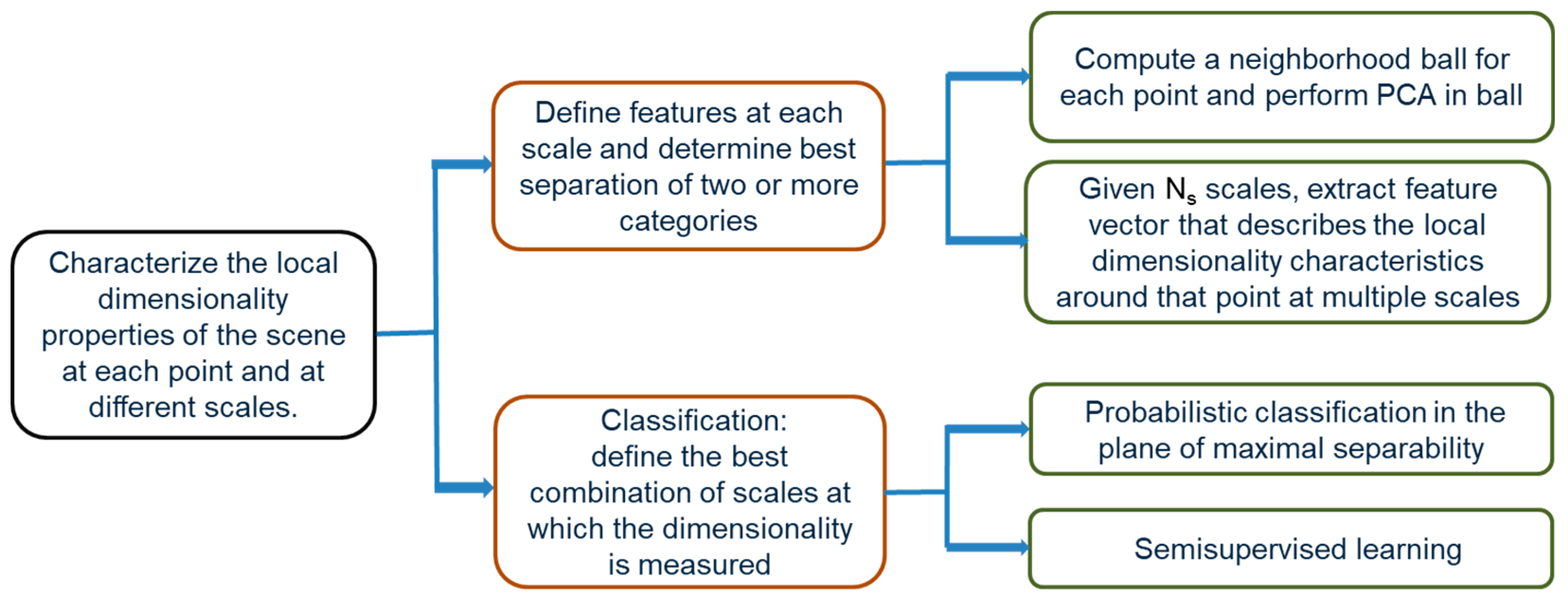
In accordance with the 3D geometric characteristics of the scene elements at multiple scales, the algorithm applied in this paper classifies the surface vegetation and road surface by means of multiscale local dimension features, which can be used to identify vegetation in complex scenes with very high accuracy. For example, this algorithm can be used to describe the local geometry of the midpoint of a scene and represent simple basic environmental features (ground and vegetation) [28]. The workflow of the multiscale dimensionality criterion algorithm is shown in Figure 2.

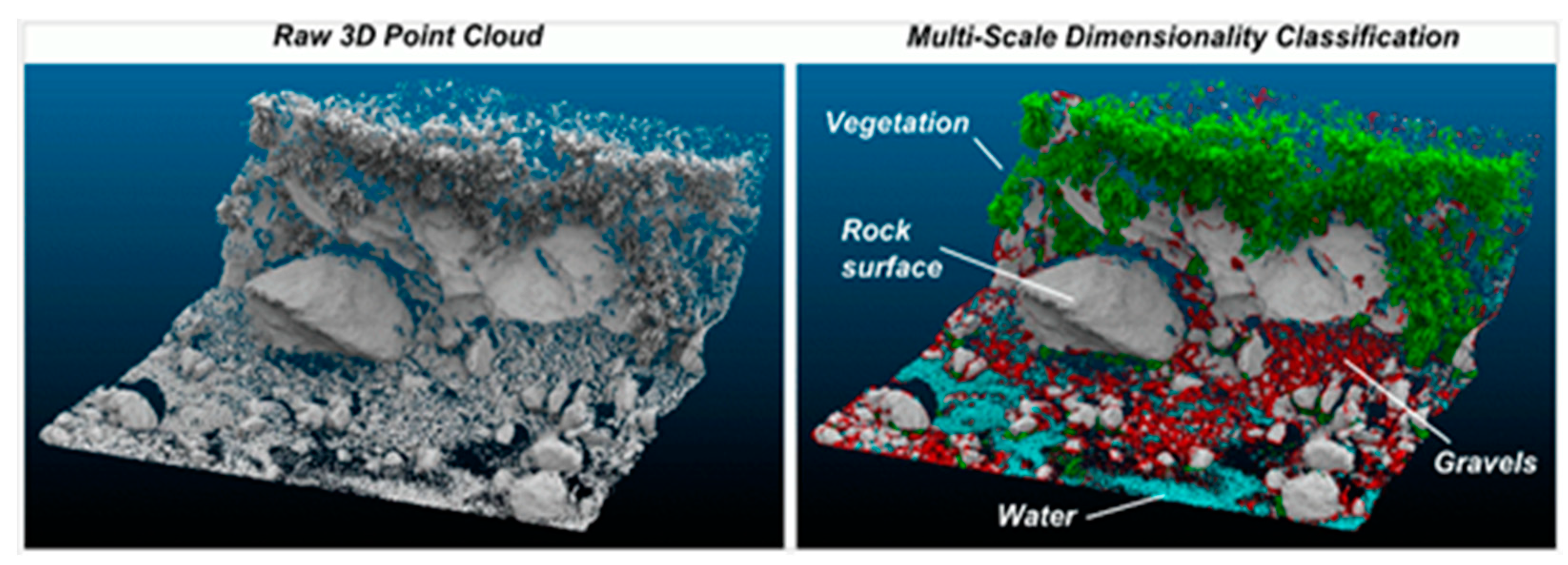
The main idea of the multiscale local dimension features is to describe the local dimension attributes of the scene at each point and different scales. For the example shown in Figure 3, when the scale is 10 cm, the rock surface looks like a 2D surface, the gravel looks like 3D objects, and the vegetation looks like a combination of 1D and 2D elements because it contains stem-like elements and leaves. When the scale is 50 cm, the rock surface still looks 2D, the gravel also appears to be 2D, and the vegetation has the properties of 3D shrubbery. By combining information from different scales, we can thus establish obvious features for recognizing certain object categories in a scene.

We define features at each scale, use training samples to determine which combination of scales enables the best separation of two or more categories, and then analyze the local dimension characteristics at a given scale. For each point in the scene, a neighborhood sphere is calculated at each scale of interest. Principal component analysis (PCA) is performed based on the recalculated Cartesian coordinates of the point in the sphere. Let λi, i = 1, 2, 3, denote the eigenvalues generated via PCA in order of decreasing size, as follows: λ1 > λ2 > λ3. The variance ratio of each eigenvalue is defined as:

pi = λi/λ1 + λ2 + λ3.

(1)

When only one eigenvalue can explain the total variance of the neighborhood ball (i.e., the variance ratio of that eigenvalue is 1), the neighborhood around that point in the scene is distributed in only one dimension. When two eigenvalues are needed to explain the variance, the neighborhood around that point in the scene is distributed in two dimensions. Similarly, a completely 3D point cloud is a cloud for which the variances of all three eigenvalues are of approximately the same magnitude. Specifying these scales is equivalent to placing a point X in a triangle field, which can be done in terms of the center-of-gravity coordinates independently of the shape of the triangle. By varying the diameter of the sphere, we can observe the shape of the local point cloud at different scales.

The features thus generated by repeatedly calculating local dimension features at each scale of interest are called multiscale features. Given N_S scales, for each point in the scene, we can obtain an eigenvector that describes the local dimension features of the point cloud around that feature point at multiple scales.

The general idea behind the classification approach is to define the best combination of dimensions for measurement such that the maximum separability of two or more categories can be achieved. We rely on a semi-automatic construction process to construct a classifier that can find the best combination of scales (note that all scales contribute to the final classification but with different weights), that is to maximize the separability of two categories, i.e., vegetation samples manually defined by the user and ground samples, for separation from the point cloud. The accuracy of vegetation classification at different scales is 99.66% [28].

3.2. Extraction Algorithm

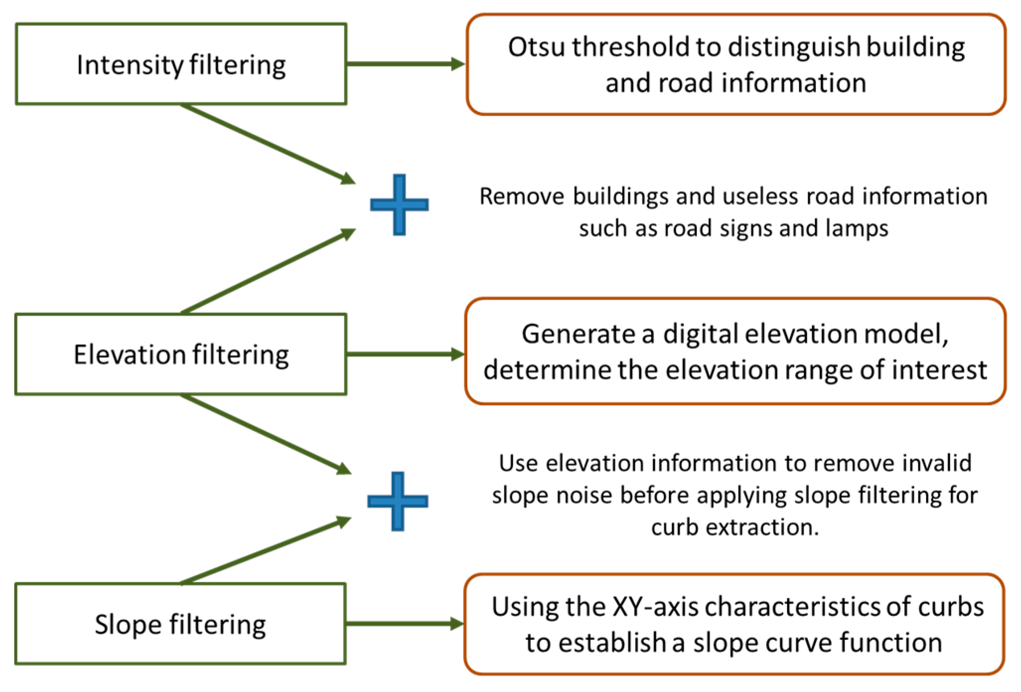
Curbs are located in the adjacent regions between roads and sidewalk/green belt areas. Curbs can be regarded as road boundaries. In general, a simple model of a road point cloud has the following characteristics: (1) Reflectivity. The material of the road surface generally consists of asphalt, cement, or concrete. Therefore, its intensity characteristics are different from those of vegetation, bare ground, etc. Vegetation will produce multiple echoes, so its reflection value will usually be higher than the echo intensity of the road. (2) Elevation. The road generally lies near the ground surface. Therefore, the elevations of road points and ground points are similar to each other and generally lower than those of the surrounding buildings, trees, and other objects. (3) Slope characteristics. Roads are normally designed in accordance with certain standards to exhibit only small changes in elevation within a small area, especially in urban areas. Therefore, the slope of the road network should be relatively small. Thus, to find the locations of curbs, the characteristics of points on each street should be analyzed using three indicators: reflectivity, elevation change, and slope change. The workflow of extraction part shows in Figure 4.

3.2.1. Intensity Filtering

Although point cloud echo intensity information is relatively vague in terms of MLS point cloud data, when the differences between the media attributes of adjacent targets are obvious, one can easily distinguish between different features, such as the surface of a street and the road marking a line in the middle of the street, by analyzing the corresponding laser echo intensity information.

Moreover, the reflection coefficient of a ground surface material, which determines the amount of laser echo energy that is reflected, depends on the wavelength of the laser, the thickness of the dielectric material, and the brightness of the surface of the medium. Although some of these parameters may vary in different locations, the land cover types considered in this study can be classified in accordance with certain general principles. Significant differences in intensity values between media allow researchers to set clear thresholds to distinguish them [29]. Among the three types of land cover considered here, lawns and trees have the highest intensity values, while roads and bare ground have the lowest. In a road environment, the road surface generally consists of an asphalt or concrete material, from which the reflection of a laser beam is low and diffuse [30]. For the mobile survey system used in this paper, Optech’s Lynx system, intensity values are provided for several different media, based on which road objects can be significantly distinguished based on the intensity distributions of the associated major object classes [17] (see

Table 1. Values of laser reflectivity of different media.

Intensity	Medium	Object Classification
1–100	Asphalt, concrete	Street, bridge
100–300	Paint coat	Road marking line
>300	Vegetation	Grass, tree

).

Due to the difference in weather conditions and different LiDAR instruments, the intensity of different objects is not constant. In this study, the statistics of reflectivity intensity of different objects (average, minimum, maximum, and standard deviation of reflectivity values of different objects in the study site) are shown in

Table 2. Statistics of intensity values.

Medium	Average Intensity	Max.	Min.	STD
Asphalt	49.193	157	9	7.817983
Building	70.120	255	3	52.15585
Grass	57.954	116	1	10.68206
Concrete	14.150	138	0	7.989562

. It can be seen from Table 2 that the average strength of buildings is the highest. In addition, the standard deviations of concrete, asphalt, and grass are relatively low.

To determine the multiple thresholds of intensity values belonging to buildings and road markings, the concept of the Otsu threshold [27] is employed in this study because it does not require user-defined parameters for determining thresholds from the histogram. The working principle of the intensity filtering is that thresholds are determined as the maximum values or maxi-mum peaks in the Otsu’s intra-class variance. The basic idea of this method is that well-thresholded classes have to be distinct with respect to the intensity values of their pixels and the converse must be true. The important property of the method is that it is based entirely on computations performed on the histogram of an image. In this way, the Otsu threshold method is used to determine the intensity value T that maximizes the variance between the background (building) and foreground (road marking) categories [31]. After threshold segmentation, the LiDAR points are divided into building points and road marking points.

The steps of road marking detection are listed below:

• Compute the normalized intensity histogram. Let $n_i$ be the value of the i-th histogram bin, and let M be the number of road points; then, the normalized intensity ($p_i$) is:

  $$p_i=\frac{n_i}{M}$$

  (2)
• The cumulative sum $P\left(k\right)$ is the probability that a LiDAR point belongs to the range $\left[0,k\right]$ and is calculated as:

  $$P\left(k\right)={{\displaystyle \sum }}_{i=0}^k{p}_i$$

  (3)
• Compute the cumulative mean intensity $m\left(k\right)$ in the range $\left[0,k\right]$:

  $$m\left(k\right)={{\displaystyle \sum }}_{i=0}^{k}i{p}_i$$

  (4)
• The global cumulative mean $m_G$ is the mean intensity of the whole histogram, where $L$ is the number of possible intensity values that the LiDAR can record:

  $$m_G={{\displaystyle \sum }}_{i=0}^{L-1}i{p}_i$$

  (5)
• Compute the global intensity variance ${\sigma }_G^2$:

  $${\sigma }_G^2={{\displaystyle \sum }}_{i=0}^{L-1}{\left(i-m_G\right)}^2{p}_i$$

  (6)
• The local variance ${\sigma }_L^2$ is the variance of a specific intensity:

  $${\sigma }_L^2=\frac{m_{G}P\left(k\right)-m\left(k\right)}{ P\left(k\right)\left(1-P\left(k\right)\right)}$$

  (7)
• The threshold T is the value of k that maximizes ${\sigma }_L^2$:

  $$T=\underset{0\le k\le R-1}{\mathrm{argmax}}{\sigma }_L^2\left(k\right)$$

  (8)

The value of T can be calculated only once or can be recalculated with each new arrival of LiDAR data. Due to the variance of the intensities of the road markings and asphalt along a street (caused by wear), we recomputed T when new LiDAR data are received.

3.2.2. Elevation Filtering

In urban areas, the elevation distribution of roads is continuous, and the terrain tends to undulate. Additionally, the range of changes in a small scanning range tends to be flat, in accordance with the characteristics of streets. In a scanned scene, the elevations of roads are generally lower than those of buildings, trees, and street lamps; thus, an elevation threshold H can be set to remove some of the nonground points (shows in Figure 5). If the height of the vehicle laser scanner is used as the threshold H, the exact value of this threshold is uncertain and depends on the vehicle type; however, this approach can prevent the elimination of good points based on changes in slope and elevation. This approach can generally be used in flat urban areas, based on the characteristics of the streets, and the study area considered in this paper can be seen to be flat from the slope measurements in the digital elevation model. Thus, elevation filtering can be achieved in this way in the study presented here.

Once the threshold value has been determined, if the elevation value of a point in the point cloud is larger than the threshold value, then that point is removed from the point cloud data. However, for points whose values are less than the threshold, then corresponding data are preserved to be used for slope filtering.

3.2.3. Slope Filtering

The slope filtering algorithm consists of two steps: pseudo scanning line generation and road edge detection.

We define the slope between two consecutive points in the generated pseudo scan line and the elevation difference of the point relative to its neighborhood in the pseudo scan line (Figure 6). First, for the point cloud perpendicular to the orbit data, we divide it into several data blocks of a given length. The outline of each data block is sliced according to a given width. Accordingly, each profile contains both points related to the road pavement and points related to objects outside the road boundary. All points of each profile are projected onto a plane perpendicular to the slice direction. In an MLS system, the frame is defined as a right-handed orthogonal coordinate system with any user-defined point as the origin. The frame orientation is fixed such that the X-axis points toward the front of the vehicle, the Y-axis points toward the right side of the vehicle, and the Z-axis points toward the bottom of the vehicle. A curb will be perpendicular or almost perpendicular to the road surface, corresponding to a sharp jump in height [32]. Therefore, we estimate the curb location in accordance with a gradient difference criterion and finally separate road points from nonroad points in this way. We assume that the slope between the road surface and road boundary will usually be larger than the slope of the continuous road surface. In addition, the elevation of a sidewalk point will be higher than that of a nearby road point.

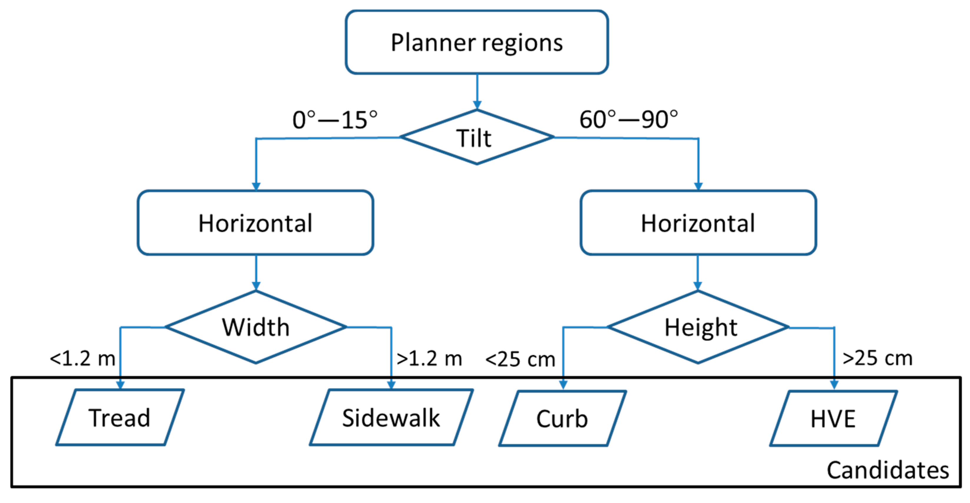
The slope difference method is used to detect curbs among off-highway points. In this work, a decision tree based on ISO-25142 [33] and experimental values were implemented to mark the regions in the preliminary category (Figure 7). Although it is impossible to establish a clear classification based on geometric parameters, ISO-25142 is listed as a good reference. According to ISO-25142 reports and street design and construction manuals from many countries indicate that curbs are generally between 1.5 and 25 cm high.

Therefore, we mathematically define the following two observations as:

$$\left\{\begin{array}{l}\mathrm{if}\left(S_{slope}>ST\&(D_{min}\le D_i\le D_{max}\right)),\mathrm{curb}\mathrm{candidate}\\ \mathrm{otherwise},\mathrm{non-curb}\mathrm{point}\end{array}\right\}$$

(9)

where S_slope is the slope of two consecutive points, S_T is a given slope threshold, and D_i is the elevation difference of a point and its neighbor. D_min and D_max are the minimum and maximum thresholds, respectively.

In our algorithm, if S_slope gets a slope greater than S_T, it means that the point has reached a possible curb. If the height difference D_i near the curb candidate is within the range of [D_min, D_max], the curb candidate will be marked as a curb; otherwise, it will be marked as a non-curb point.

3.3. Curb Refinement

Since the curbs extracted by the above method are sparse in the test area, the next task is to refine the curb edges. We generate smooth edges from these curb points by refining the road boundary.

Balado [34] proposed a curb refinement based on split and merge operations. But the effect is not satisfactory in irregular occlusion such as cars. We use the quadratic Bézier curve spline to fit the curb boundary line segment, which converts the road boundary point into a road boundary curve with topological information.

The curb to be refined is classified into straight line and curve. If reconnected road edges are collinear, the curbs are connected by straight lines. If reconnected road edges are not collinear, the curbs are connected by curve fitting (Figure 8). Extend the edge of the road to the intersection, and then reconnect the extension line into a Bézier curve.

The Bézier curve is the parameter path traced by function B(t) for the given points P₀, P_1, and P₂. The reconnection process can be written as a problem of finding the three control points of the Bézier curve. Points P₀ and P₂ are the start and endpoints of the smooth area respectively.

B(t) = (1 − t)²P₀ + 2(1 − t)tP₁ + t²P₂, t∈[0,1]

(10)

If the curbs of the two parts are collinear, then P₁ is in the middle of P₀ and P₂. If the curb to be reconnected is not collinear, place P₁ at the intersection of the two-point tangent projection lines of P₀ and P₂. The non-collinear area of the curb produces a parabolic segment.

3.4. Curb Clustering

The KNN algorithm is an object classification algorithm based on the nearest training samples in the feature space. In the classification process, unlabeled query points are simply assigned the same labels as their K nearest neighbors. Usually, an object is classified by majority vote according to the labels of its K nearest neighbors [35].

If K = 1, the object is simply classified as belonging to the class of the object closest to it. In the case of binary classification (two data classes), it is better to use an odd integer value of K to prevent the fuzziness of the classification results due to similarity between the two data classes [36]. After converting each image into a fixed-length real vector, we use the most common distance function for KNN classification, called the Euclidean distance:

$$d(x,y)=||x-y||=\sqrt{\left(x-y\right)·\left(x-y\right)}={({{\displaystyle \sum }}_{i=1}^m{\left(x_i-y_i\right)}^2)}^{1/2}$$

(11)

where x and y are histograms in X = RM.

Due to the discontinuities of section lines that can be caused by occlusion by vehicles, pedestrians, or trees, a process of inspecting and checking the results of boundary extraction is needed to obtain accurate road boundaries. For this purpose, according to the characteristic that the curb is extended but the curb occlusion is not extended, KNN clustering is used to cluster the candidate road points into multiple groups. In actual situations, due to curbs and pedestrian occlusion, the data is non-Gaussian or cannot be linearly separated. By evaluating the distance between training samples (for example, Euclidean distance, Manhattan distance), It can be classified by the KNN algorithm.

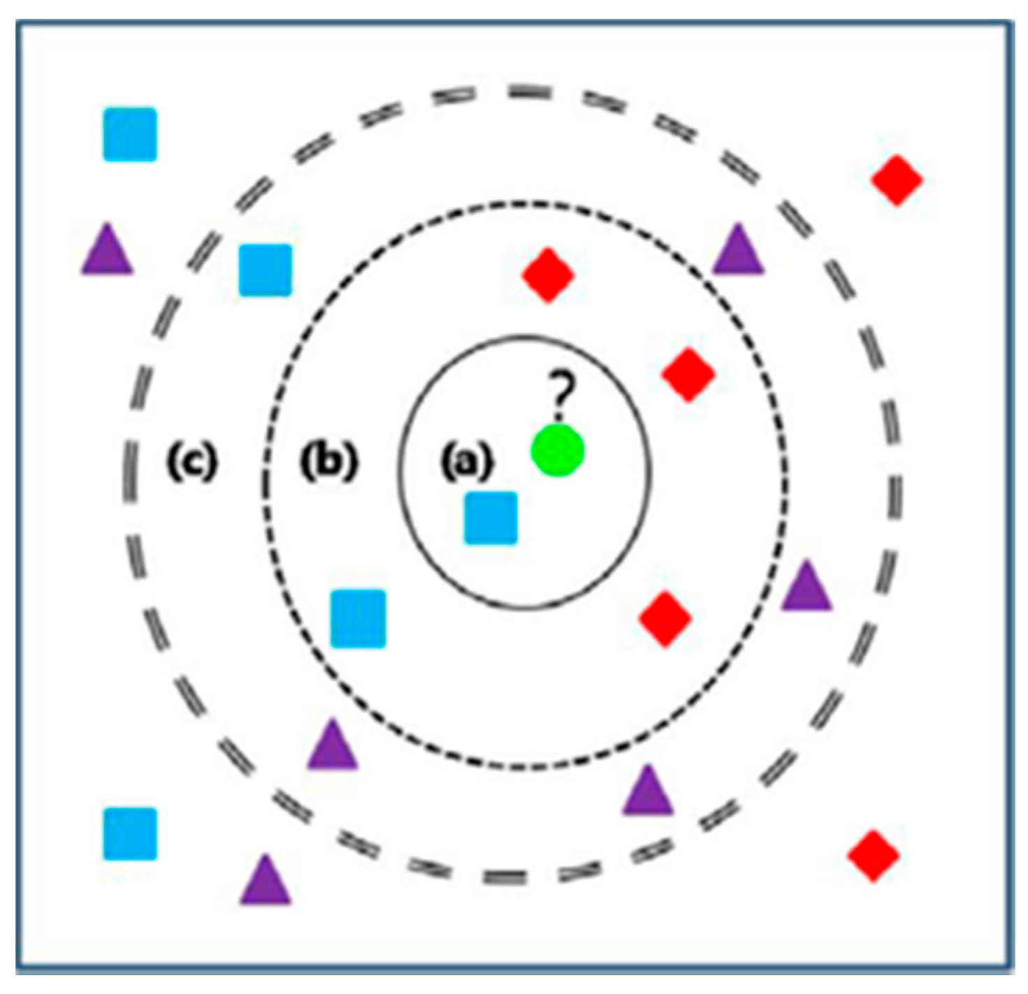
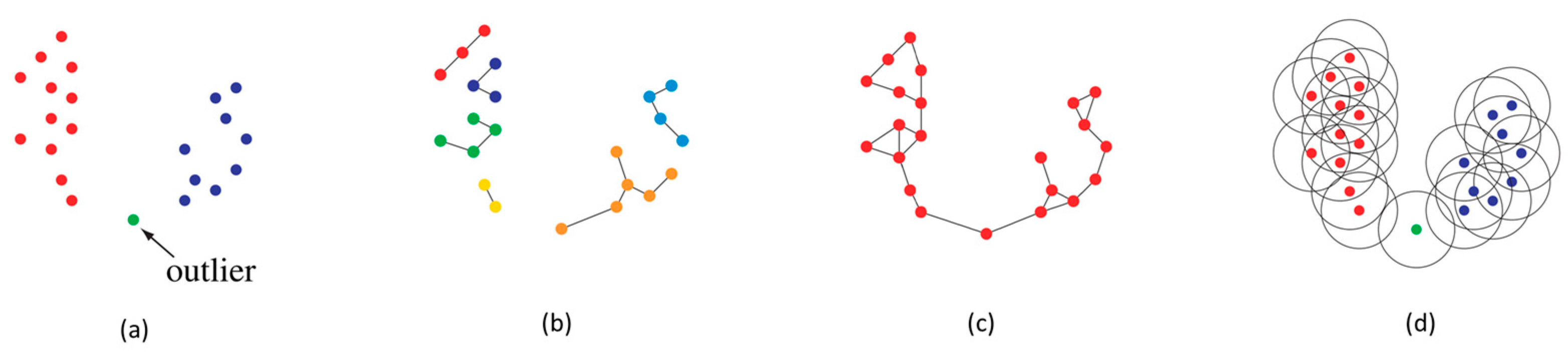
The traditional KNN method improves the clustering accuracy by selecting the K value. The values of the K parameters are chosen by trial. In the case of binary classifications (two data classes), it is better to use an odd integer K to prevent similarity in the dominance of the two data classes, which can cause ambiguity of the classification results. Figure 9 visualizes the process of KNN classification, In the example depicted in Figure 9, the query point is represented by a circle. Depending on whether the K value is 1, 5, or 10, the query point can be classified as a rectangle (a), a diamond (b), or a triangle (c), respectively. In this article, we use Radial Bounded Nearest Neighbor Graph (RBNN) to cluster laser data. Unlike traditional KNN, it connects each node to its K nearest neighbor, regardless of distance. Each node is connected to all neighbors located in a predefined radius r. The set of edges in the RBNN graph is:

E_RBNN = {{x_i, y_i, d_xi,yi|d_xi,yi ≤ r}

(12)

Figure 10 shows the difference between KNN and RBNN in terms of segmentation capabilities. We set a basic 2D data set with two clusters and a noisy point. Given the correct r as a parameter, the RBNN method separates the two clusters and outliers from each other well. However, 1-NN produced 6 clusters (include six kinds of color in subfigures (b)), 2-NN produced only one cluster (only has one color in subfigures (c)). The NN algorithm with numbers as parameters not only did not separate the two clusters but also did not identify noisy points. The main advantage of using the RBNN method is that we do not need to perform the nearest neighbor query for each node, and it does not involve graph cutting and graph structure rearrangement.

The RBNN algorithm is an effective method of removing some pseudo boundary points through clustering. By clustering the extracted boundary points, it is possible to detect pseudo boundary points belonging to cars, green belts, fences, etc. Additionally, it is useful for extracting street curbs in an urban area because it should be possible to assemble the remaining clusters into straight lines. Thus, pseudo boundary points belonging to objects such as cars and humans can be detected and removed.

4. Data Acquisition

In this paper, the instrument that was used to obtain accurate data for curb extraction is named ROBIN.

The ROBIN measurement system includes a high-accuracy laser scanner. The laser pulse repetition rate (PRR) is up to 550 kHz, the wavelength is 1064 nm, the intensity recording is 16 bit, and maximum vertical field of view is 360 degrees, maximum measurement rate is 1000 kHz. The accuracy and precision of the instruments are 8 mm and 5 mm, respectively.

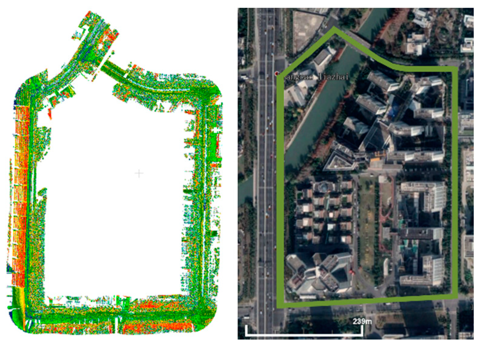
The data for this project were collected on 23 November 2018, in Shanghai where is around the Zhangjiang region and close to the Guanglan Road subway station. The 3D digital urban map obtained using Google Earth is displayed in Figure 11. The length of the total data set is 1693.41 m. The storage size of point cloud data is 1.63 G, with a total of 35 million points.

This article mainly extracts the curbs of complex three-dimensional urban scenes. The three complex scenes include vegetation covering the curbs, curved curbs, and occlusion curbs (see Figure 12). The study sites used in this project included streets, curbs, grass, trees, buildings, and road markings. It should provide a concise and precise description of the experimental results, their interpretation, as well as the experimental conclusions that can be drawn.

5. Analysis and Discussion

5.1. Visual Examples of the Obtained Results in Classification Process

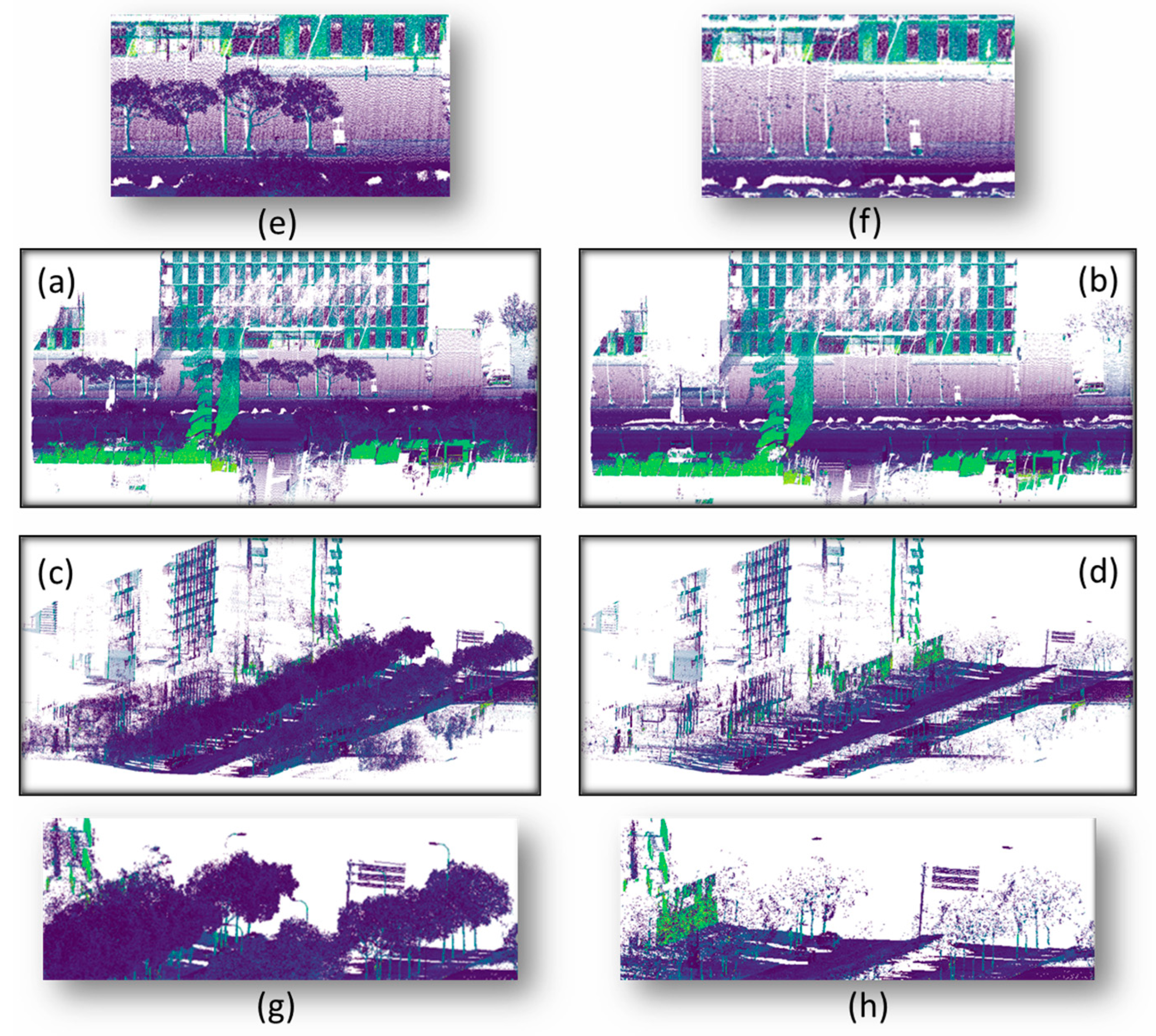
The multiscale dimension criterion classification algorithm is applied to this experimental scenario, and the results of multi-scale dimensionality criterion classification are displayed in Figure 13.

In this experiment, from qualitative evaluation, most of the vegetation information was identified from the classification results of the two places shown in the figure above. Through quantitative calculation, the accuracy of vegetation extraction is 92.11%, and the Fisher’s discriminant ratio is 4.1925.

5.2. Visual Examples of the Obtained Results of Curb Extraction

In order to visually analyze the results obtained in the test area, the detected curbs have been superimposed on the point cloud in the study area. The test site corresponds to the street section of Shanghai, China. This is a typical urban area, with roads that have structured boundaries in the form of crosswalks and curbs and ramps in garages. Most of the curb on this street is covered with vegetation, which creates shadows in the point cloud and obscures the curb, making the detection of curbstones challenging. The number of points in the clouds is 37 million.

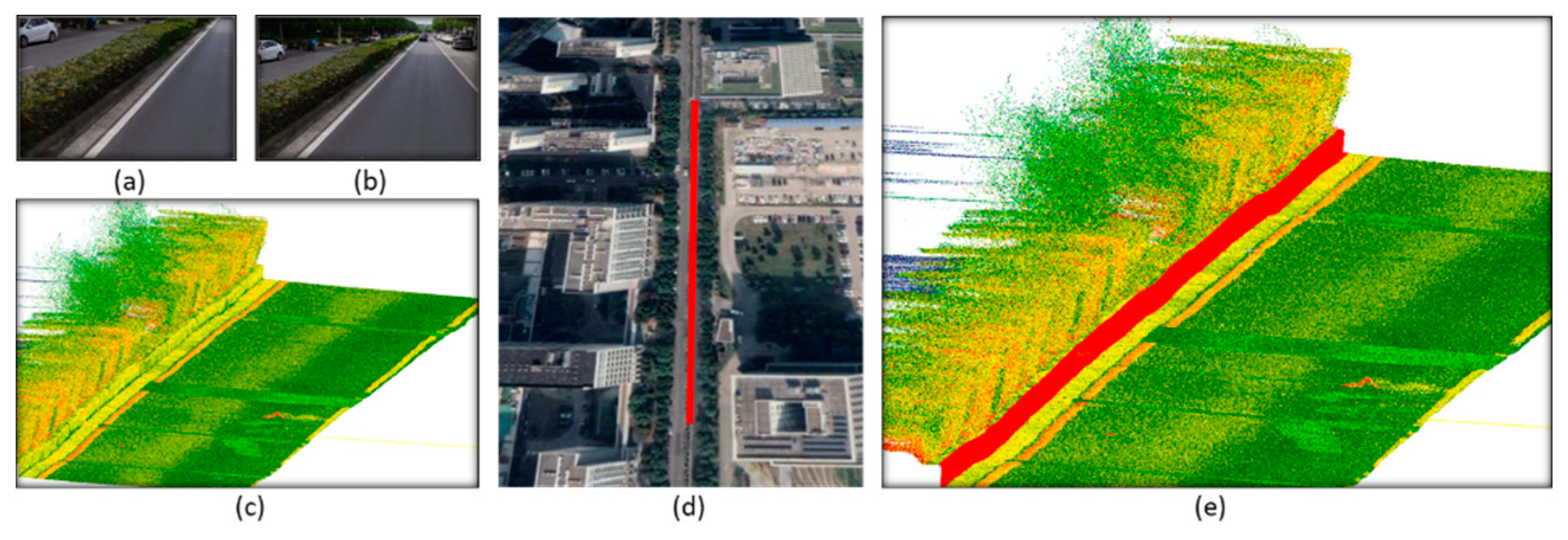
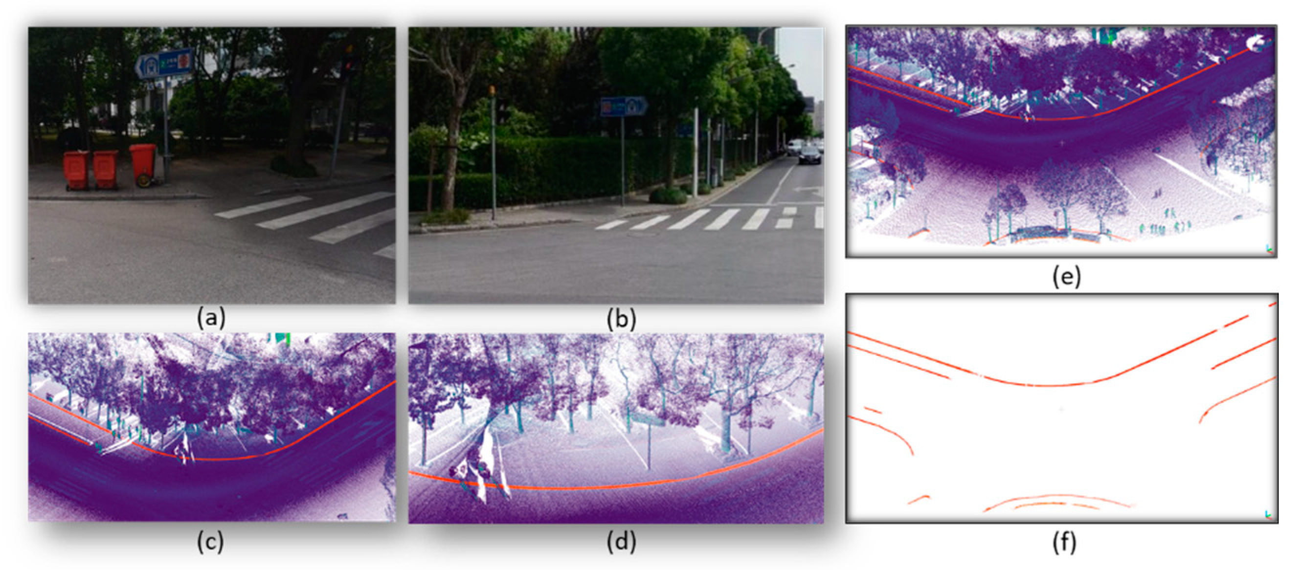
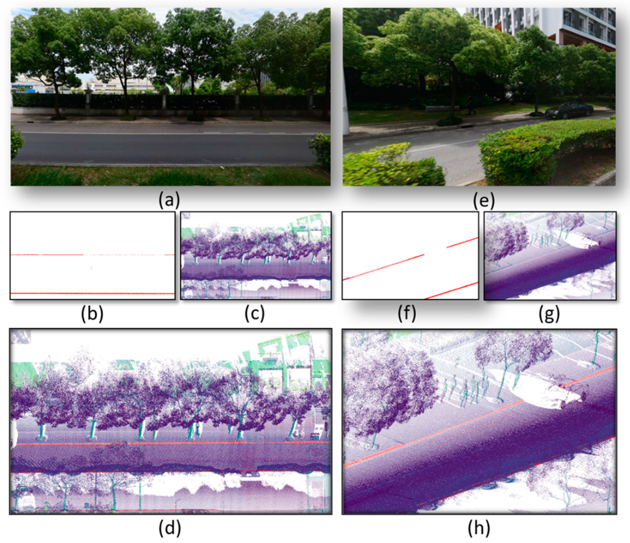
The results of the curb edge segmentation method are fully shown in the following three sections: Figure 14, Figure 15 and Figure 16. Figure 14 represents the curb extraction result on curbs covered by vegetation, Figure 15 is the curb extraction result of the curved part of the street, and Figure 16 is concentrated on the street with intermittent curbs. For each detail, three images are displayed: the street view, the original point cloud of the detail, and the segmentation result.

The curbs of the streets at several study sites are displayed in Figure 14, Figure 15 and Figure 16. We can clearly see the curbs, which are marked with red points. The extracted road curbs were superimposed on the MLS point clouds for visual inspection. Different parts of the test data sets were enlarged for detailed examination. This paper mainly presents the results of extracting, vegetation covering above curbs, straight curbs, and curved curbs at intersections in an urban road environment. By considering the extracted edge point cloud in combination with the real 3D map of the study sites, our analysis shows that the proposed method can effectively detect curb points even at positions where the vegetation covering the curb. At an intersection, the proposed algorithm not only clearly distinguishes between the motorway and sidewalk but also achieves strong closure of the whole curb on a curved surface. In areas where a laser point cloud can be obtained (excluding the inaccessible laser points on the backs of features due to the data acquisition route), the curb information that can be seen in the real 3D scene map can be successfully identified and extracted.

Following the entire processing method, we can observe that the proposed algorithm can be widely used in urban areas because the study sites chosen in this study are typical of such environments. The study sites include buildings, trees, grass, asphalt roads, concrete roads, road markings, and so on. Moreover, the results for the study sites prove that in areas without curb information, no data will be extracted and identified as curbs. Therefore, the proposed method is suitable for the extraction of street curbs in urban areas.

5.3. Quantitative Evaluation

We conduct a quantitative analysis by comparing the automatic extraction line and the manual extraction line. In order to evaluate the accuracy of curb detection, we manually extracted the road boundary from the original point cloud. We analyze these extracted curbs, and the length of reference is the total length of the edge in the experimental area.

Table 3. Parameters after overlaying the manually extracted.

	Left Edges	Right Edges
Length of reference (Manual extraction according to field survey)	1691.2	1623.7
Minimum (m)	0	0
Maximum (m)	0.179	0.112
Mean (m)	0.023	0.011
Median (m)	0.015	0.009
Horizontal RMSE (m)	0.142	0.060
Vertical RMSE (m)	0.071	0.014

lists the parameters after overlaying the manually extracted curbs and the curbs extracted by the algorithm proposed in this paper. It includes the minimum distance, the maximum distance, the average, the median, and the average horizontal and vertical root mean square error (RMSE) between the edge extracted by the algorithm and the manually extracted edge.

Based on the visual information and geometric information, we successfully extract the left and right edges of the test area. The results of road edge extraction show high accuracy, which is attributable to the use of uniform and dense point cloud data along the road. The maximum distance between the extracted left and right edges and the actual edge is approximately 0.1 m, and the average and median distance between the right edge and the actual edge is less than 0.01 m. Guan et al. [37] reported mean horizontal and vertical root mean square error (RMSE) values of 0.08 m and 0.02 m, respectively, for curbs extracted from MLS data. In this paper, the horizontal and vertical RMSE values of the extracted right edge of the road segment are 0.060 m and 0.014 m, respectively. There is a large gap in the effectiveness of the method proposed in this paper between left and right edge extraction. The main reason for this gap is that the laser scanner only travels in one direction when obtaining data on the road. Due to the occlusion of the street by trees in the middle of the road, some data are lost, and the accuracy of the left edge is lower than that of the right edge. When the Otsu threshold is used to classify the intensity information, we can use a more intelligent algorithm and propose more reasonable parameter settings, which increases the effectiveness of distinguishing the road surface from its edge and improves the accuracy of road edge extraction. However, the proposed street curb extraction method needs to be further tested on long road areas to verify its effectiveness compared with existing methods.

In addition, to quantitatively assess the street curb extraction, we calculate the following two accuracy metrics, which are widely used for the evaluation of road extraction algorithms [38]: Completeness = TP/Lr and Correctness = TP/Le, where Lr is the total length of the reference road and Le is the total length of the extracted road. Completeness is defined as the length of the extracted line in the buffer divided by the length of the reference line. Correctness is defined as the length of the extracted lines in the buffer divided by the length of all extracted lines. TP = min(Lme, Lmr), where Lme is the total length of the extracted road that matches the reference road and Lmr is the total length of the reference road that matches the extracted road. A buffer is established on both sides of the reference road, and each point of the extraction results is marked as lying inside or outside of the buffer.

The completeness and correctness values obtained for the study sites considered in this paper are given in

Table 4. Completeness and correctness at two study sites.

Buffer Width (m)	Completeness (%)		Correctness (%)
	Left Edges	Right Edges	Left Edges	Right Edges
0.1	88.3	88.5	87.9	90.6
0.2	93.7	94.2	94.9	96.4
0.3	98.5	98.7	98.8	98.6
0.5	99.2	99.8	99.6	99.7

.

The completeness and correctness values from the study sites are shown for buffer widths of 0.1 m, 0.2 m, 0.3 m, and 0.5 m. Buffer width probably gives an idea of the level of accuracy of the extracted data, which seems to be probably around half a meter. When the buffer width is 0.5 m, the correctness value for the left edges and right edges are 99.6% and 99.7% respectively. Among them, because the distance between parked cars or other elements above the curb is very short, the length of the curb that is not detected on the left and right sides of the road by the proposed method accounts for 0.8% and 0.2% of the total length of the curb. Due to the false extraction caused by elements with geometric shapes similar to the curbs (such as the underside of the car and the stairs), the left and right edges also have a false extraction rate of 0.4% and 0.3%, respectively.

5.4. Comparison with Other Methods

All experiments were performed on a 3.70 GHz Intel Core i7-8700K processor with 16 GB RAM. The calculation time of the whole algorithm in this paper is about 45 min. In order to prove the effectiveness of the proposed method, the following latest technologies are used for comparison, we set the buffer width to 0.5 m. The results are shown in

Table 5. Compared with the results of other methods.

	Kumar (2013)		Yang (2013)	Sun (2019)	Zhang (2018)	Proposed Method
	Left Edges	Right Edges				Left Edges	Right Edges
Completeness (%)	96.5	65.4	95.13	95.1	93	99.2	99.8
Correctness (%)	100	63.8	98.09	95	92.5	99.6	99.7

.

In 2013, Yang [19] and Kumar [39] described the most advanced method for street curb extraction. Zhang [8] and Sun [40] subsequently proposed superior street curb extraction methods by using the geometric or spatial information of urban area edges. The evaluation and comparison results are listed in Table 5. It is clear from the results in the table that the proposed method achieves the best performance.

As shown in Table 5, the completeness of the proposed method is 99.2% at the left edge and 99.8% at the right edge, and the correctness is 99.6% and 99.7%, respectively, which is better than other methods. In addition, between left and right edges, there is only a small difference in the accuracy of the proposed road boundary detection, which reflects the robustness of the proposed algorithm.

Kumar et al. [39] used a new combination of the gradient vector flow (GVF) method and a balloon parameter active contour model to extract road edges from the ground moving LiDAR data. However, the internal and external energy parameters used in the algorithm are selected based on experience, and its robustness must be determined through experimental analysis. For edges extracted from MLS data, the average integrity and accuracy of the Kumar method are 96.5% and 100%, respectively. For edges with a buffer width of 0.5 m, the average integrity and accuracy are 65.4% and 63.8% respectively.

In Yang’s [19] method, MLS point cloud data are regarded as continuous scan lines, non-circular points are filtered by a sliding window operator, and curb points are detected based on a curb pattern. However, it is difficult for Yang’s method to distinguish between asphalt and soil, asphalt and vegetation, and asphalt and grass embankments. In addition, the length of the sliding window used to filter the non-circular points also affects the detection of the road area. If the length of the window is less than the width of the curb, points near the curb may be incorrectly marked as curb points. By comparison, the proposed algorithm has better robustness and good extraction accuracy and correctness for straight roads, curved roads, and intersections.

Zhang’s [8] method is similar to Sun’s [40] method. It uses the nearest neighbor on the same laser line to calculate the smoothness and continuity of the midpoint in the local area and then searches for the boundary points with road boundary features on each laser line. His method can achieve good results on flat roads and slopes with small curvature. However, Zhang used the boundary point search method. When the direction of the car is different from that of the road boundary or the curvature of the road is large, Zhang’s method can only search the boundary points closer to the vehicle. Sun’s method is an improvement of Zhang’s method. For situations in which there are obstacles on the road and the shape of the road boundary is irregular, the algorithm still has high accuracy in extracting road boundaries. However, Zhang’s method does not make use of the intensity information of the point cloud and is vulnerable to interference from roadside grass. In addition, the robustness of the algorithm is low, and incorrect extraction occurs easily in areas without road edges.

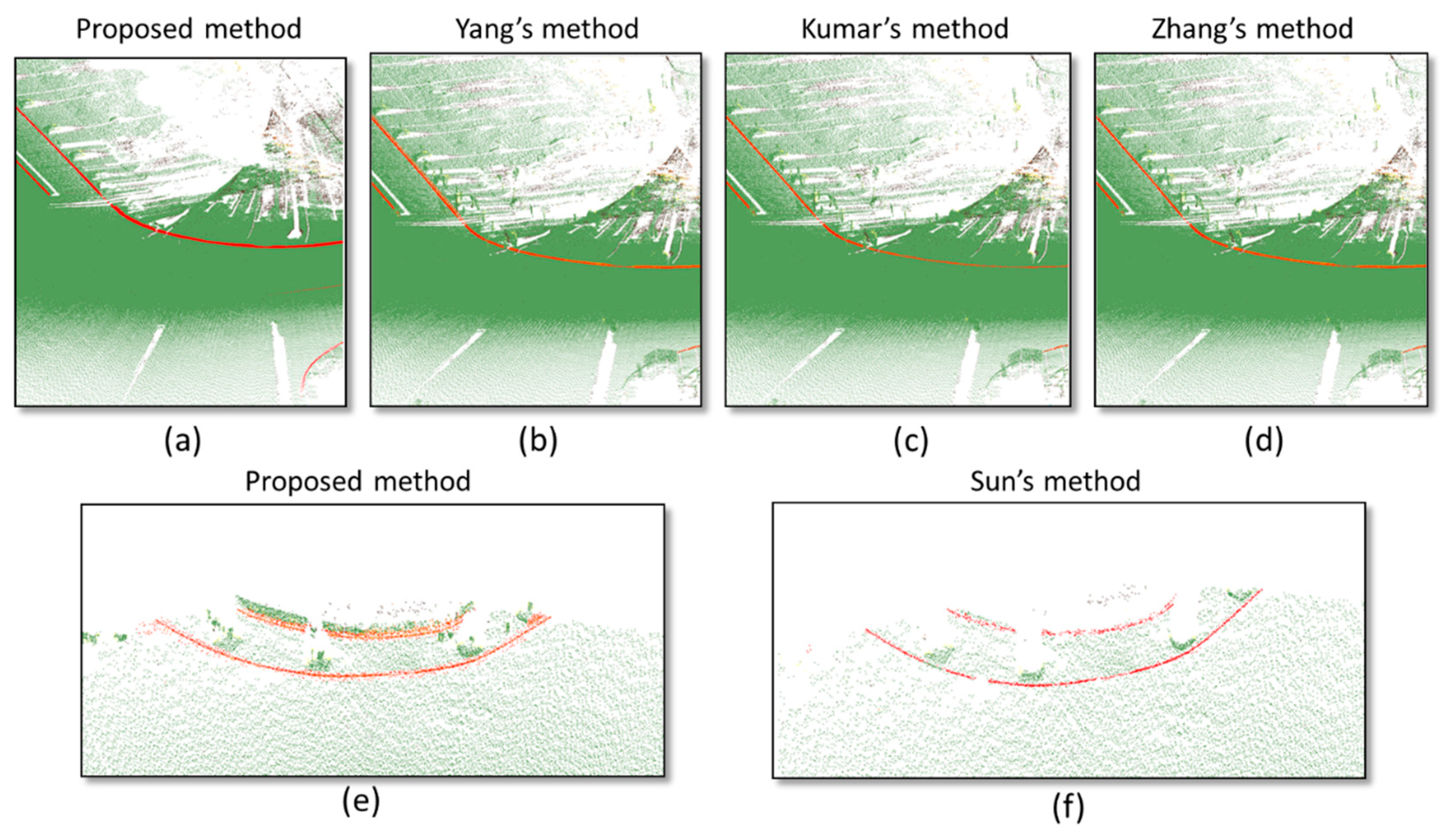
We tested their four techniques on our data sites, and the extraction results are shown in Figure 17. In the straight street scene, due to the simplicity of the road, the results of all methods are similar. In the curve scene, we can see that the point cloud extracted by Kumar based on the gradient vector flow (GVF) method at the edge of the curve is too sparse (Figure 17c). In Yang’s method, the short curbs cannot be recognized in our experimental scenes. This is mainly because Yang’s algorithm relies on the choice of the length of the sliding window (see Figure 17b). In Zhang’s method, the street curbs are far from being extracted when the road curvature is too large, so the extraction result in Figure 17d is not outstanding. Sun’s method is an improvement to Zhang’s method and has higher accuracy on curved roads. However, Sun’s algorithm is easily affected by grass on the roadside. Because there is grass cover above the curb, the completeness of curb extraction is not high in Figure 17f. In contrast, the curb point extraction method proposed in this paper performs better.

The excellent performance of the proposed method is mainly because of three capabilities: (1) by considering the existence of obstacles on the road and using the spatial attributes of the road boundary, it can adapt to different heights and different road boundary structures; (2) it uses both spatial information and geometric information and thus exploits the different advantages of spatial information and geometric information in edge extraction to reduce the robustness of street curb extraction; (3) the RBNN clustering algorithm used to fit the road boundary has better adaptability to different road boundary shapes, especially large changes in the curvature of the road boundary.

6. Conclusions

In this paper, a new method of extracting street curbs is introduced. First, multiscale dimensionality classification is performed to classify and extract street point cloud data. Subsequently, the characteristics of elevation, echo intensity, and slope change are used to detect the street curbs from the accurate LiDAR point cloud. Then, the quadratic Bézier curve spline is to refine the curb edges. As the last step, the RBNN clustering algorithm is used to cluster the extracted boundary points and remove some pseudo boundary points. In three complex urban scenarios (vegetation covering the curbs, curved curbs, and occlusion curbs), this article verifies the reliability and robustness of its algorithm in the experimental part.

Although street curbs are extracted with a high level of correctness using the proposed algorithm, there are two limitations of this study that need to be mentioned. On the one hand, at the study sites considered here, there were some weaknesses in the intensity filtering results. In attempts to identify the problem in the intensity filtering process at the study sites, it was found that the intensity values recorded from asphalt roads, grass, buildings, and road markings are all highly similar, whereas vegetation objects such as trees and grass do not produce quite such high values, as noted in a previously cited reference. Therefore, the filtering results are not entirely clear. The Otsu threshold [27] method can be used to calculate a general value for distinguishing between buildings and road markings, but it does not work well across all possible situations. This is one of the limitations of the method presented in this paper, and overcoming this limitation is a topic for future work.

On the other hand, the second limitation is related to the settings for slope filtering. This method will not work well in high-slope areas. If the slopes at all study sites were approximately 1 m, the slope threshold would be set to approximately 0.2–1.2 m. In this way, we could easily remove buildings and streetlamps from the high-elevation parts of high-slope study sites, but all information would be preserved in low-elevation areas with elevation values below 1.2 m. Notably, there seems to be a considerable amount of noise in low-elevation areas, including the information recorded from cars operating in the middle of the street and people walking in the street.

To summarize the two limitations detailed above, this algorithm can be successfully applied in flat areas and under conditions in which the intensity values of buildings and street markings can be readily discriminated. However, further consideration will be needed in the future to develop an algorithm that can be applied in arbitrary areas with diverse terrain conditions. Furthermore, as the equipment has integrated imagery, we will involve the fusion of sensors in the future.