Spatio-Temporal Estimation of Biomass Growth in Rice Using Canopy Surface Model from Unmanned Aerial Vehicle Images

Abstract

The awareness of spatial and temporal variations in site-specific crop parameters, such as aboveground biomass (total dry weight: (TDW), plant length (PL) and leaf area index (LAI), help in formulating appropriate management decisions. However, conventional monitoring methods rely on time-consuming manual field operations. In this study, the feasibility of using an unmanned aerial vehicle (UAV)-based remote sensing approach for monitoring growth in rice was evaluated using a digital surface model (DSM). Approximately 160 images of paddy fields were captured during each UAV survey campaign over two vegetation seasons. The canopy surface model (CSM) was developed based on the differences observed between each DSM and the first DSM after transplanting. Mean canopy height (CH) was used as a variable for the estimation models of LAI and TDW. The mean CSM of the mesh covering several hills was sufficient to explain the PL (R² = 0.947). TDW and LAI prediction accuracy of the model were high (relative RMSE of 20.8% and 28.7%, and RMSE of 0.76 m² m⁻² and 141.4 g m⁻², respectively) in the rice varieties studied (R² = 0.937 (Basmati370), 0.837 (Nipponbare and IR64) for TDW, and 0.894 (Basmati370), 0.866 (Nipponbare and IR64) for LAI). The results of this study support the assertion of the benefits of DSM-derived CH for predicting biomass development. In addition, LAI and TDW could be estimated temporally and spatially using the UAV-based CSM, which is not easily affected by weather conditions.

1. Introduction

Obtaining knowledge about the dynamic of plant biomass is an essential part of precision agriculture, as such information aids in the management decision making, risk assessment and the design of labor-saving and efficient technologies and that can compensate for the physical deficiency in the agricultural labor force [1,2,3]. Aboveground biomass (total dry weight: TDW) estimation has been widely explored due to its direct relation to crop yield commonly by farmer’s expert knowledge and destructive sampling which are not timely and labor efficient. The consequences thereof leading to lower productivity [4,5]

Alternatively, the potential of satellite-based remote sensing for crop management has been widely studied [6]. However, satellite imaging is hindered by coarse resolution, cloud cover and fixed-timing image acquisition, which may not synchronize with some specific phenological phases [7,8]. In addition, information on sufficient resolution and apt revisit frequency for precisely mapping smallholder farm units has been a challenge until the influx of unmanned aerial vehicles (UAVs) [9]. The low cost, high flexibility, simple handling and high spatial resolution of UAVs enable their application in many fields of research including biology, forestry and hydrology [10,11,12,13,14,15,16,17,18]. Recent studies based on vegetation indices (VIs) extracted from the images captured by relatively inexpensive UAV-based digital and multispectral cameras have been used to examine many options for crop growth indices [19,20]. However, it has been established that the normalized difference vegetation index (NDVI), widely used in remote sensing, saturates the index values as the growth stage progresses, affecting its sensitivity to genetic and environmental conditions in the acquisition of high-resolution data [20,21].

The emergence of UAV photogrammetry has facilitated the on-demand generation of high-resolution datasets such as the Digital Surface Model (DSM) [22]. Comparatively, DSM generated from UAV photogrammetry offers advantages such as easy handling of the UAV platform, the likelihood of adapting sensors, user-friendly data evaluation tools, accessibility of difficult terrains and low cost, over terrestrial platforms or the light detection and ranging (LiDAR) [23,24,25]. Differing from satellite imagery, the DSM generated from overlapped aerial images is relatively less affected by the weather and time zone, except by strong winds and rainfall at the time of the filming. The spike in the use of UAVs for image acquisition proceeded simultaneously with the onset of a novel photogrammetric technique known as structure-from-motion (SfM), which together with multi-view stereo (MVS) provides a robust system capable of creating high-resolution DSMs using less expensive cameras [26,27,28,29].

DSMs have been used extensively in agriculture for monitoring important traits such as plant height, yield and biomass estimation in major crops such as maize, rice, barley, potato and even perennial grasses such as Miscanthus giganteus [30,31,32,33,34]. However, little information is known of studies conducted on rice paddy fields and their particularities which highlights significant varietal differences among cultivars. Additionally, the fact constrains the location of control points (differing from dry land), could lead to potential correlation errors in SfM due to water reflections. Even though, investigations into several other factors that affect DSMs from UAV photogrammetry such as image quality, the layout of the Ground Control Point (GCPs), flight altitude among others have been carried out [35,36,37]. However, the analysis of time-series dynamic processes of various allometry and phenology mechanisms and their relationship with a different environment in rice has not been well studied. For these reasons, rigorous efforts to redress these information gaps are needed.

Unquestionably, previous works have made significant contributions to improve the feasibility of DSM application in agriculture by outlining various prospects, methodologies, challenges and mitigation strategies. However, lapses in the available information for estimating crop growth under various environmental conditions using this method require significant attention especially in a homogeneous canopy such as rice fields. Hence, in this study, UAV photogrammetry was used to assess the time-series aerial growth dynamics of different paddy rice varieties under different environmental conditions to improve the estimation of and biomass growth from canopy height using the DSM. Obtaining such data is a good step towards designing precise phenological calendars that are variety specific to feed crop estimation models. Linear regression models based on the DSM and extrapolated from overlapped RGB images were developed to estimate crop growth. From the estimated results of LAI and crop biomass, the differences in the planting year and growth conditions were revealed using DSM instead of VIs, especially under various conditions, with high spatio-temporal resolution.

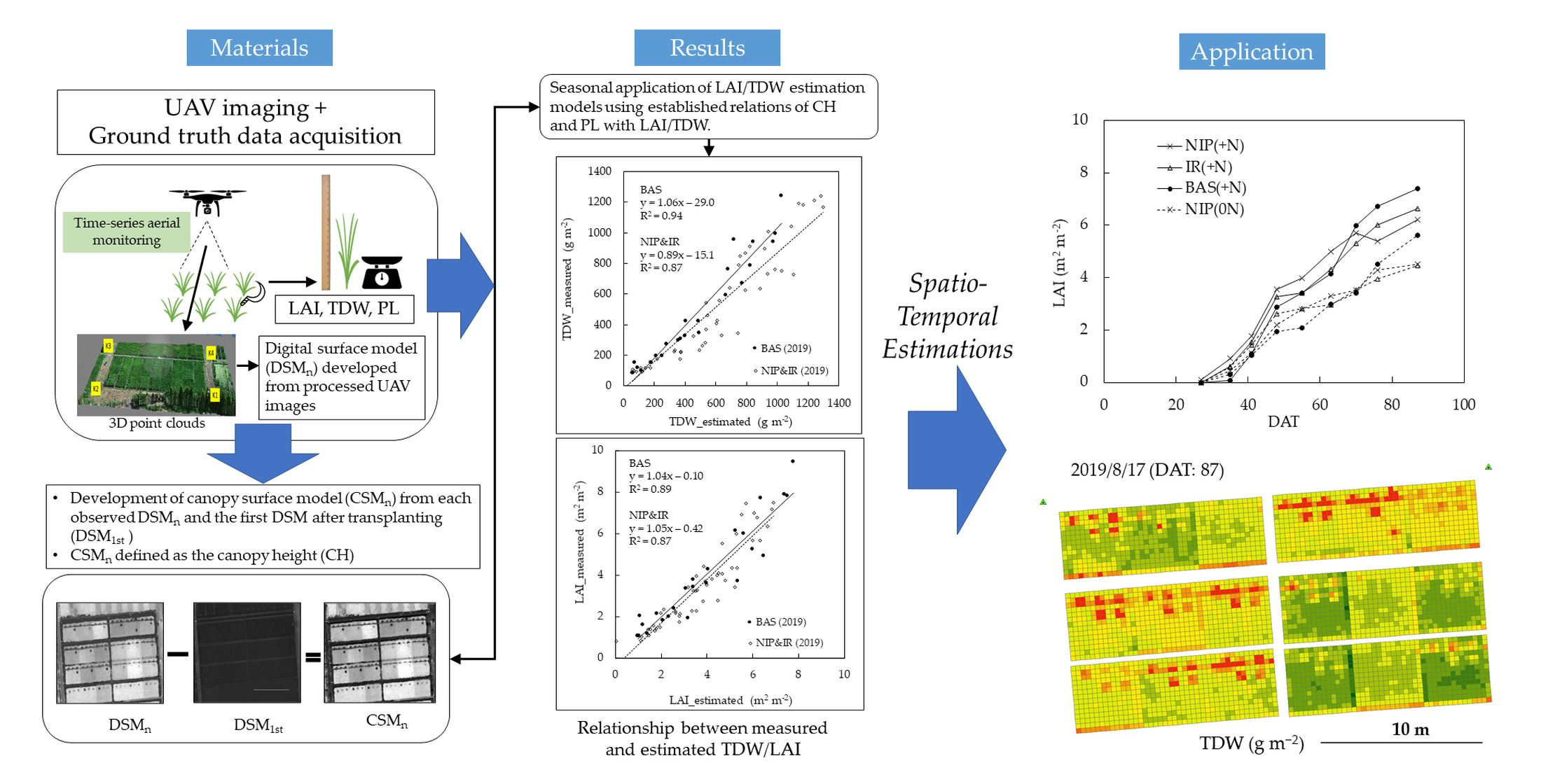
2. Materials and Methods

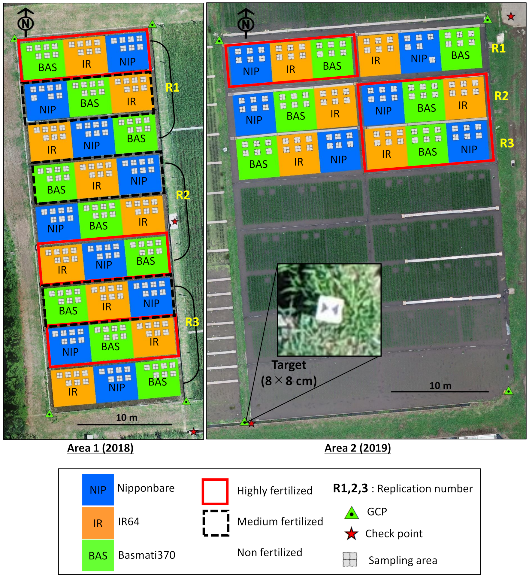
2.1. Experimental Site

Two field experiments were conducted during the summers of 2018 and 2019 as shown in Figure 1 (hereinafter referred to as Area 1 and Area 2, respectively) in a paddy field containing alluvial clay loamy soil, on the farm belonging to the Tokyo University of Agriculture and Technology (35°39′57″N, 139°28′16″E, 49 m above sea level). The climatic conditions of this area are mild and generally warm, with a mean annual temperature and precipitation of 15 °C/59 °F and 1530 mm, respectively [38]. Areas 1 and 2 measured 45 m × 15 m and 15 m × 27 m, respectively, and were arranged in a randomized complete split-plot block design, with three replicates each, with fertilizer treatment as the main plots and rice varieties as sub-plots.

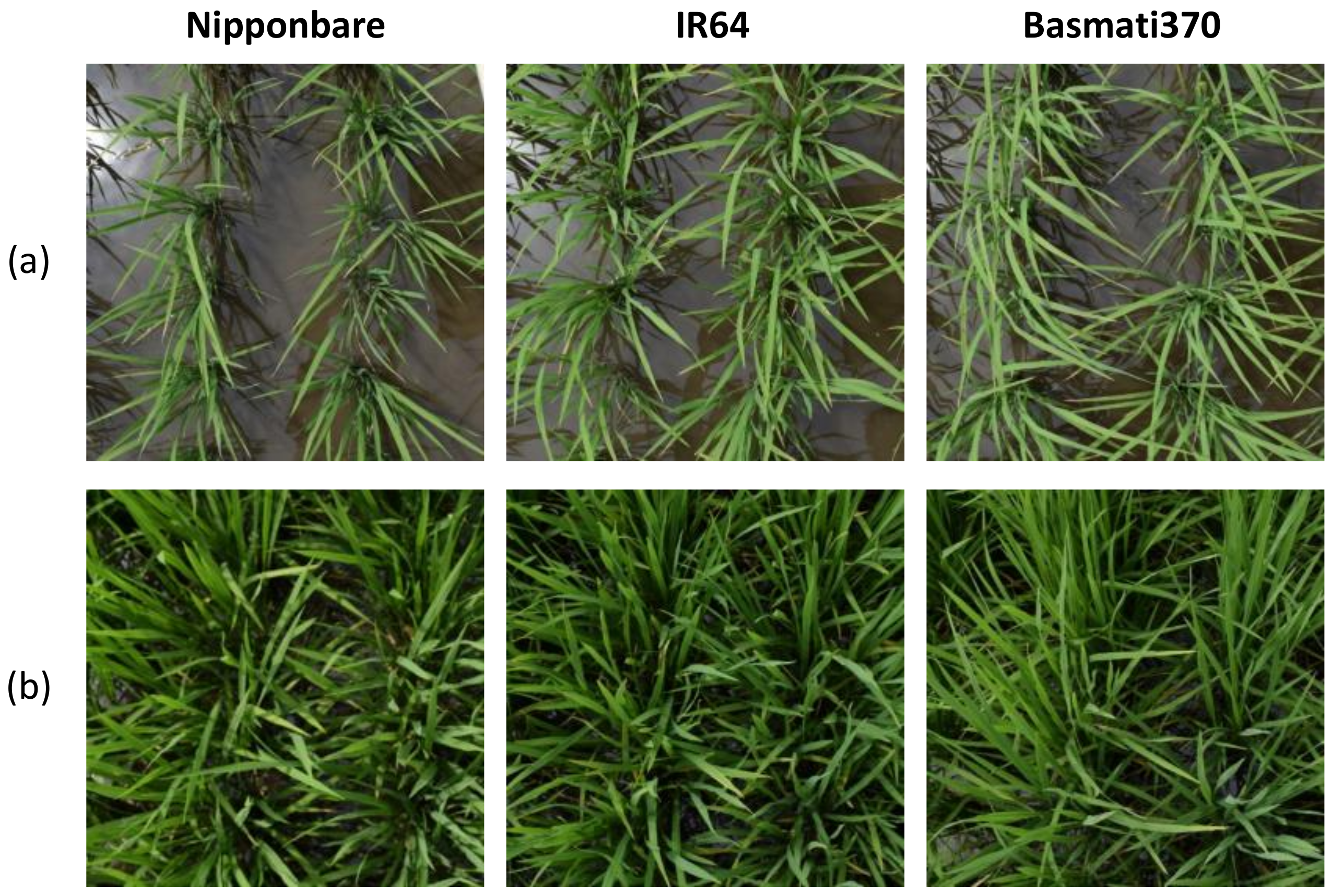
2.2. Rice Cultivars and Fertilizer Application

Three rice cultivars—Nipponbare (Japonica), IR64 (Indica) and Basmati370 (Indica) were used based on their wide genotypic variability. Nipponbare is the first japonica cultivar in the world whose genome sequence has been sequenced in 2004 and was used as a representative of japonica varieties [39]. IR64 is the most widely cultivated indica variety in the world and was used as a representative of indica varieties [40]. Basmati370 is a traditional indica variety of aromatic rice with relatively less genetic improvement [41]. It was used in this study because the traditional (less genetically improved) varieties tend to show vigorous vegetative growth, and the plant morphological traits are very different from the improved varieties such as Nipponbare and IR64 [42]. Seedlings at the fourth leaf stage were transplanted at a hill spacing of 15 cm × 30 cm with one seedling per hill. The transplanting dates were 30 May 2018, in Area 1, and 22 May 2019, in Area 2. Nitrogen fertilizer was applied in three and two splits in 2018 and 2019, respectively. Fertilization in 2018 was divided into no fertilization, low fertilization (basal: 3 g m⁻², and topdressing 3 g m⁻²) and high fertilization areas (basal: 3 g m⁻², and topdressing 3 g m⁻² × 6 times). For 2019, the plots were divided into non-fertilized (0N) and fertilized (+N) areas (basal: 2 g m⁻², and topdressing: 2 g m⁻² × 6 times). Phosphorous pentoxide (P₂O₅) and potassium oxide (K₂O) were also applied at a ratio of 10:10 g m⁻² as the basal dose for each plot (17.5% P and 60% K concentrations, respectively).

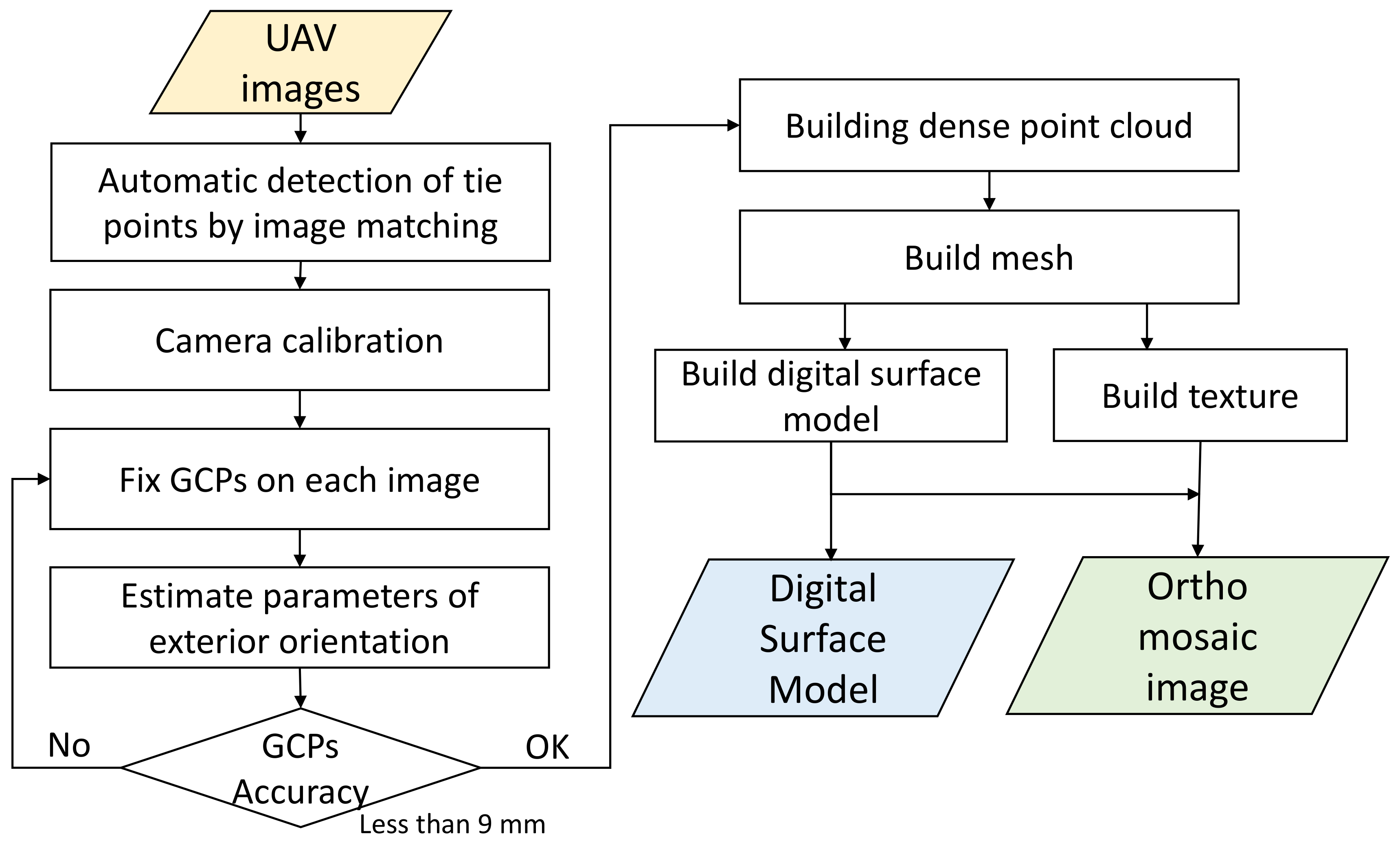
2.3. Aerial Image Acquisition

Ground control points (GCPs) were established in both experimental fields using the total station and auto level by conducting traverse surveying and levelling. The coordinates of the GCPs were referred to the Japan Geodetic Datum 2011/Plane Rectangular Coordinate System zone 9 as a map projection, and the GCPs were set at the four corners of each field (Figure 1). A set of overlapped images of the fields was taken using a UAV (Inspire 2; DJI, Shenzhen, China) equipped with an RGB camera (Zenmuse X4S; DJI, Shenzhen, China) with 20 megapixels (5472 × 3648 resolution). The flight altitude was fixed at 30 m above the rice canopy with a forward and lateral overlap rate of 85%. Approximately 160 images were acquired during each flight campaign, and the flight survey was performed at two-week intervals in 2018 (eight flights) and weekly intervals in 2019 (eleven flights). For time-series monitoring, the aerial survey was achieved weekly in 2019 to acquire more detailed phenological changes in rice growth. In case of the occurrence of rain or strong winds, the shooting time and dates were altered accordingly. Due to the predominant flooded conditions in the paddy field at the early stages, it is better to take the UAV images at the time when the sun altitude is not high.

2.4. Ground Truth Data Collection

Plants were harvested from a 60 cm × 60 cm area that covers eight standard hills from each plot (Figure 1). A total of 27 and 18 plots were sampled in 2018 and 2019, respectively per each sampling date. The total number of samples was 189 (27 plots × 7 times) and 108 (18 plots × 6 times) for up to 89 and 87 days after transplanting in 2018 and 2019, respectively to examine TDW, LAI and PL. Figure 2 shows an example of images of three cultivars taken on 3 and 27 July, and the area of the photos almost correspond to the sampling area covering eight hills per plot. The above-ground parts of the plants such as leaf blades and stem plus leaf sheaths were retained, while the roots were discarded. PL was obtained by straightening the plants one at a time and measuring the height from the ground surface level to the tip of the rice plant. The PL was measured simultaneously along with the CH on each UAV survey Day. Leaf area was obtained by measuring randomly sampled, fully expanded and healthy laminae, based on in situ area measurement using an automatic leaf area meter (AAM-9A; Hayashi Denko, Tokyo, Japan) with a conveyer belt assembly. After determination of leaf area, the plant organs were oven-dried at 80 °C for 72 h to attain a constant dry weight, after which their dry weights were measured. The specific leaf area was calculated as suggested by San-oh et al. [43], after which the LAI, on a ground area basis, was calculated.

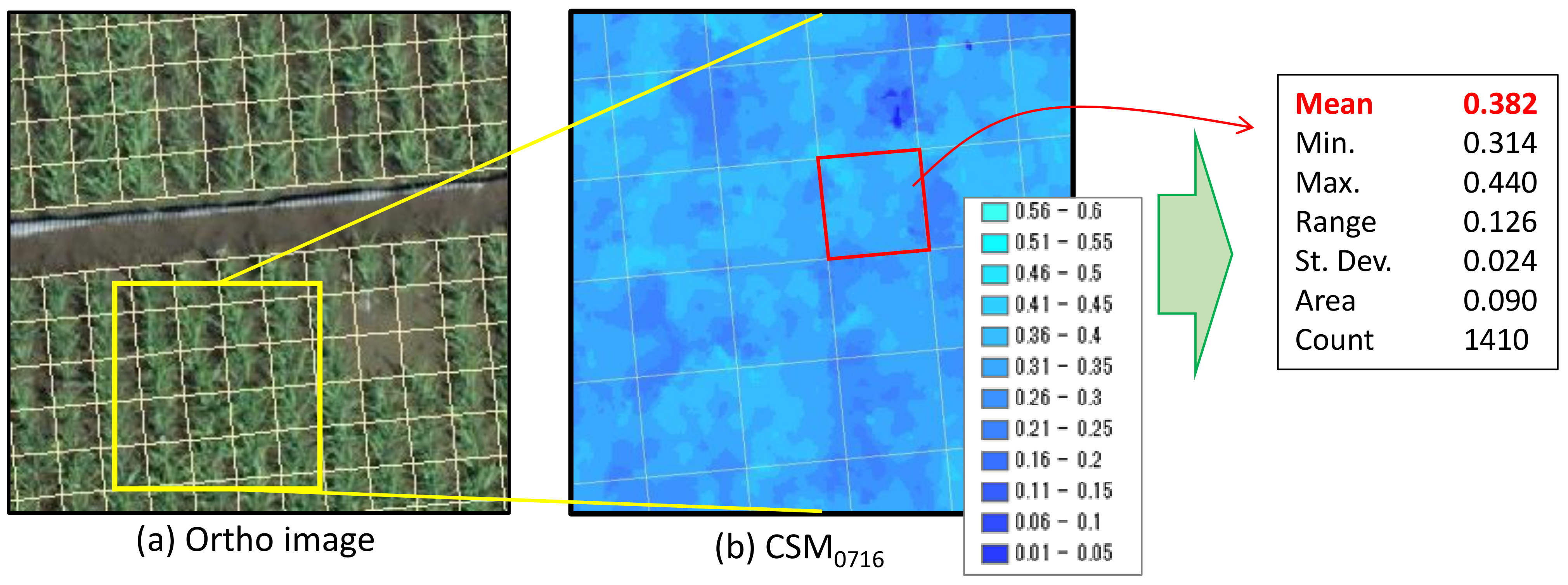
2.5. Generation of the Digital Surface Model and Canopy Surface Model

The Agisoft Metashape Professional (ver. 1.5.1), an SfM software, was used to generate a 3D point cloud, ortho-mosaic images and DSMs by processing the UAV-acquired images. This approach, as outlined by Gindraux et al. [44], supports the simultaneous processing of overlapped images using the geometric constraints of camera positions. Hereinafter, the DSM is also referred to as the canopy surface model (CSM) because it reflects the crop surface. The process of generation of DSM and ortho mosaic image as explained by Yamaguchi et al. [45] was used in this study as shown in Figure 3.

First, tie points were automatically identified from the overlapped aerial images; then the tie points were used to calibrate the camera parameters such as the focal length of the lens, principal point positioning and radial and tangential distortions. The parameters of external orientation (camera position and tilting angle) were estimated using the detected tie points and the four installed GCPs, and a dense point cloud was generated. This processing was performed to achieve a GCP accuracy within 1 pixel. A DSM and an ortho mosaic with a spatial resolution of approximately 9 mm/pixel were developed. The standard deviations of the z-coordinate (elevation) at the two checkpoints each year (Figure 1) were examined from the generated time-series DSMs and were ±8.4 mm and ±18.4 mm in 2018 and ±4.9 mm and ±4.5 mm in 2019. From this, it was confirmed that the DSM generated using the minimum number of 4 GCPs required for photogrammetry showed sufficiently robust and stable in the use of the analysis of crop height.

Using the DSM, CSM was calculated from the distance between the DSM of each observation day (DSM_n) and the first DSM after transplanting (DSM_1st) [46]. DSM_1s can be regarded as almost flat inside the paddy field and is defined as the reference plane to generate CSMs. At this time, since the paddy is flooded, the influence of the refraction of water may be included in the z-coordinate, but this was a systematic error and was not corrected. The value of the CSM was defined as the canopy height (CH). This relation is mathematically expressed as:

$${\mathrm{CSM}}_n={\mathrm{DSM}}_n-{ \mathrm{DSM}}_{1\mathrm{st}},$$

(1)

where n represents the observation dates.

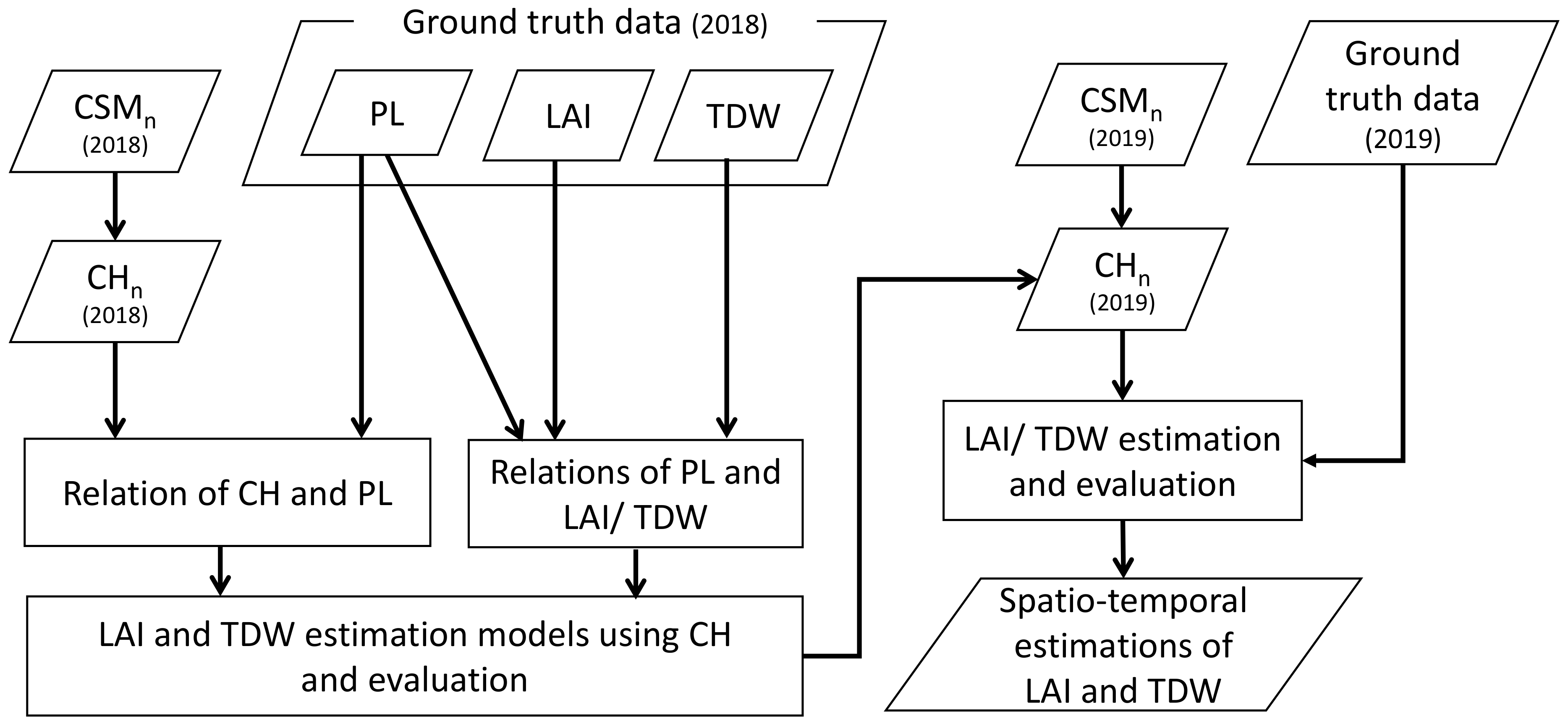
2.6. Procedures of Spatio-Temporal Estimation of Biomass Growth

Using CSM and ground truth data collected in 2018 and 2019, we developed the models to estimate LAI and TDW from CH in relation to PL and tried to estimate LAI and TDW spatially and temporally. Figure 4 shows the flowchart of spatio-temporal estimation of biomass growth using the CSM. First, we examined the method of calculating CSM in 2018 and derived the relations with PL. in addition, the relations between PL and LAI/TDW were derived, and from these relation formulas, LAI and TDW estimation models using CH as the variable were derived and evaluated. Furthermore, these models were applied to CH in 2019 to estimate and evaluate LAI/TDW and estimated LAI and TDW spatially and temporally.

3. Results and Discussions

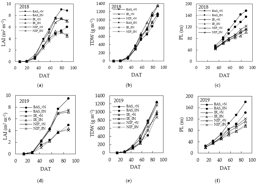
3.1. Seasonal Variations in Rice Growth

This study analyzed the potential of UAV-based DSM for monitoring crop growth, with an emphasis on developing estimation models to predict the growth of three rice varieties grown under varying environmental conditions. The results demonstrated the feasibility of using CSM-derived canopy height to predict biomass growth in rice cultivars. The approach used is uncomplicated, practicable and can achieve timeliness compared to the conventional destructive sampling method. Even though the droopy nature of rice leaves makes it difficult to measure accurately using UAVs in the field, the high correlation with the ground truth data shows a high degree of accuracy in using this technology. A growth survey on plant indices was conducted on the three rice cultivars, and the variations in their results are presented in Figure 5. The agronomic parameters investigated in this study yielded similar per-unit area values over the growth period compared to those of the other authors [47,48,49] (Figure 5a–f). Shoot biomass reached approximately 1334 g m⁻² and 1242 g m⁻² in Nipponbare and IR64, respectively (Figure 5b,e), which are characteristic of the influence of genotype and environmental conditions [50].

LAI increased almost linearly, especially under nitrogen fertilization conditions until after heading, in all varieties (Figure 5a,d), and this result agrees with Yoshida et al. (2010), who emphasized the importance of fertilizer application in enhancing LAI growth [51]. PL showed a similar increasing tendency, except for Basmati370 (Figure 5c,f). Nitrogen fertilization plays a pivotal role in rice growth because of its involvement in physiological processes such as LAI development and biomass growth. The data collected exhibited large variations in each parameter, as described above, and plant height could be obtained throughout the growth period. It can be inferred that nitrogen fertilizer had a significant effect on LAI, TDW and PL (Figure 5).

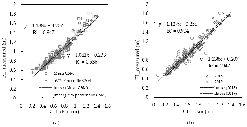
3.2. Relation between the Measured Plant Length (PL) and UAV Canopy Height (CH_dsm)

Generally, CH is relatively lower than PL because CH represents the entire canopy surface and not necessarily the highest point of the plant when measured from the field [30]. The increase in CH can be calculated from the height differences between successive CSMs using the maps obtained, as shown in Figure 6. At the early growth stages, a homogeneous canopy growth pattern was observed, which changed at the later growth stages. The results of the recorded CSMs indicate the suitability of the model developed to estimate CH with a high spatial resolution (approximately 9 mm) and accuracy as opposed to the spaceborne remote sensing approach [52,53,54]. In Figure 7, two types of CH calculated from CSM_n using the values at the 97^th percentile [55] and the mean values of a 60 cm × 60 cm area that covers eight hills are presented. As seen in Figure 7a, the two types of CH strongly correlate with PL, and the determination coefficient (R² = 0.947) of the mean CSM shows a little higher than the 97^th percentile (R² = 0.937). Furthermore, the root mean square errors of the mean and the 97^th percentile of CSM were 0.067 m and 0.074 m respectively. From these results, a complicated method is not required to derive representative CH in this case, and it implies that PL can be estimated simply using the mean of CSM.

The model accurately predicted PL in agreement with the conventional meter rule measurement method (R² = 0.947 and 0.904 in 2018 and 2019, respectively) as sown in Figure 7b. The strong linear correlations between the predicted and measured datasets of 2018 and 2019 (Figure 5) indicate a high accuracy in the model application. When deriving the estimation formula of LAI and TDW from CH, the relational formula of PL and CH in 2018 (y = 1.1384x + 0.207) was used (Figure 7b). Even though constraints such as underestimation by UAVs exist as reported, the results showed enhanced accuracy compared to that of earlier reported models [45,46].

3.3. Canopy Height Calculation

Variations in pixel units make it difficult to estimate crop growth accurately. Therefore, as shown in Figure 8, ortho-mosaic and CSM images were developed, and the entire field was divided into polygons of 30 cm × 30 cm square meshes (2 plants) from which the mean value of the plant height of each mesh was used as the representative value. The model developed was then applied to the representative values of each mesh to estimate the growth in 2019.

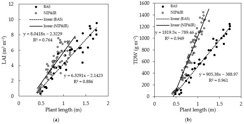
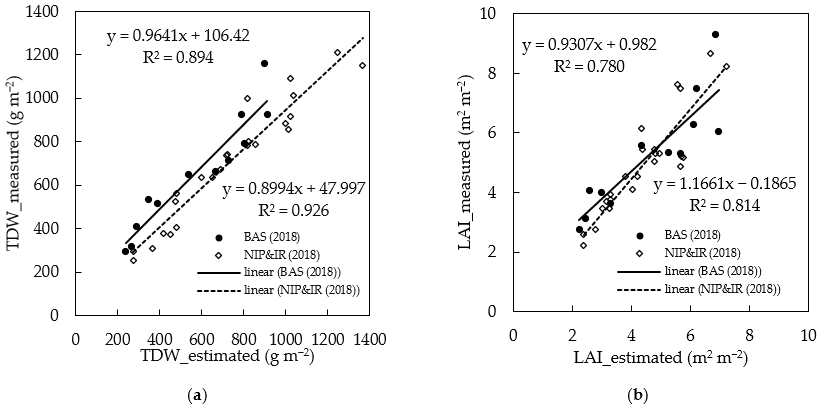
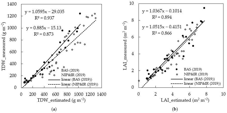
3.4. Biomass Modelling and Evaluation

The dataset was further divided into two; datasets of replications 1 and 3 were for the model calibration (n = 48) and replication 2 was used for the model validation (n = 24). A linear regression model was then developed to compare the PL with LAI and TDW and was evaluated using their coefficient of determination values (Figure 9). The calibration data for LAI yielded R² values of 0.886 and 0.764 for Basmati370, and Nipponbare and IR64 combined, respectively (Figure 9a). Aboveground shoot biomass recorded a high R² value of 0.961 in Basmati370 (Figure 9b). A similar correlation between biomass and plant height has been previously reported [56,57,58]. The effect of fertilizer on the relationship between PL and LAI/TDW was not significant in this study (Figure 9), so we regarded it as negligible because we could develop the same regression lines for the parameter. From the observed linear relationship between the PL and CH, and the relationship of PL with LAI and TDW, a model for estimating LAI and TDW from the CH was developed using the two types of relational expressions expressed below:

Nipponbare and IR64:

$${LAI}_{nipir}=9.15CH-0.66$$

(2)

$${TDW}_{nipir}=2071.3CH-412.8$$

(3)

Basmati370:

$${LAI}_{bas}=7.21CH-0.83$$

(4)

$$TD{W}_{bas}=1030.7CH-201.6$$

(5)

Basmati370 had different relational expressions compared to the other cultivars; therefore, different models were built for Basmati370 and the other two cultivars using ArcMap. Relatively, Basmati370 is less genetically improved than the other two cultivars used in this study, and generally, less genetically improved rice varieties tend to have higher nitrogen requirements and become taller compared to genetically improved rice varieties.

The derived model from the validation dataset was used to estimate LAI and TDW, as shown in Figure 10, and the results were compared with measured values considering their strong relationship with plant height. The correlation between measured and estimated values was high in TDW (R² between 0.894 and 0.926) as compared to LAI (R² between 0.780 and 0.814). In rice canopies, where leaves overlap during canopy closure, leaf area estimation could be hindered as segregation of individual tillers and leaf blades become difficult, which could result in underestimation [59]. Again, the scattering of values increased with the progress in vegetative growth, especially in LAI.

The aerial survey campaign was suspended on 27 August because of strong winds from a typhoon that resulted in the lodging of some plots; thus, subsequent surveys became challenging. Therefore, the CSMs up to 17 August was used for the estimation. The influence of lodging on the development of different cultivars could be a major limiting factor in the application of CSM [30].

Table 1. Estimation accuracy of leaf area index (LAI) and total dry weight (TDW) in 2018 (Rep. 2).

	LAI (m2 m−2)		TDW (g m−2)
	BAS	IR and NIP	BAS	IR and NIP
Mean	5.24	4.96	657.8	708.5
Mean error	−0.67	−0.55	−85.9	25.9
RMSE	1.09	0.93	119.0	84.4
Relative RMSE (%)	20.8	18.8	18.1	11.9

RMSE, root mean square error; BAS, n = 12; NIP and IR, n = 24.

shows the estimation accuracy of the LAI and TDW on the validation dataset that was set in 2018. The root mean squared error (RMSE) of LAI was approximately 1.0 m² m⁻² for all varieties. The RMSE of TDW was approximately 119 g m⁻² and 84 g m⁻² for Basmati370 and the other two varieties, respectively. The relative RMSE of estimating LAI and TDW was approximately 18% to 20% and 12% to 18%, respectively, for all cultivars. The results indicated the ability of plant height derived from the DSM approach to predict crop growth.

In 2019, the regression model derived from the validation dataset of 2018 was applied and evaluated based on the relationship between the measured and predicted values of LAI and biomass (Figure 11). As shown in Figure 11a, the prediction of aboveground dry biomass had the highest R² value (R² = 0.937) in Basmati370 with an RMSE of 0.76 (

Table 2. Estimation accuracy of LAI and TDW in 2019 (Rep. 1, 2 and 3).

	LAI (m2 m−2)	TDW (g m−2)
Mean	3.66	442.9
Mean error	0.13	55.3
RMSE	0.76	141.4
relative RMSE (%)	20.8	28.7

). Compared to 2018, the LAI distribution was slightly smaller in 2019 (R² = 0.894 to 0.866 (Figure 11b) in Basmati370 and the two other cultivars. However, the values tended to be more scattered toward the estimated LAI and TDW compared to the measured values. This is the result of bad weather conditions experienced in the early stages of the growing season, which had adverse effects on the plants. Cloudy weather conditions caused about 80% reduction in the average daylight, which reduced from approximately 7.9 h in 2018 to 1.5 h in 2019. Under cloudy weather conditions, which results in reduced solar radiation, plants tend to elongate more rather than increase their net biomass weight, and several studies assert this assumption [60,61,62]. This implies that as the environment changes, there may be a need to modify the model to fit the environment.

The estimation accuracy of the model applied in 2019 showed that there was an improvement in LAI, as shown in Table 2. Even though there was a reduction in the mean, which decreased from approximately 5.0 in 2018 to approximately 3.7 in 2019, the RMSE improved from 1.0 in 2018 to approximately 0.8 in 2019, with little variation between the years. As mentioned earlier, this result seems to suggest that the estimation results of 2018 tend to be underestimated.

Regarding the accuracy of TDW estimation in 2019, a significant mean reduction from 657.8 g m⁻² in 2018 to 472.6 g m⁻² was observed in Basmati 370 (

Table 3. Estimation accuracy of LAI and TDW for three rice cultivars in 2019 (Rep. 1, 2 and 3).

	LAI (m2 m−2)		TDW (g m−2)
	BAS	NIP and IR	BAS	NIP and IR
Mean	3.93	3.53	472.6	503.0
Mean error	−0.04	0.22	0.9	82.5
RMSE	0.79	0.75	88.3	161.5
relative RMSE (%)	20.1	21.2	18.7	32.1

BAS: n = 24, NIP and IR: n = 48.

). The RMSE of Nipponbare and IR64 in 2019 (161.5 g m⁻²) was approximately twice that of 2018 (84.4 g m⁻²), indicating a large variance between the two seasons. The relative RMSE increased from 18.1% in 2018 to 18.7% in Basmati370 in 2019 (Table 3). In 2018, 12 samples were used to evaluate the accuracy compared to the 24 samples used in 2019. Since the number of samples was large, the model fitted well with the variation, which was evaluated to be relatively small as the accuracy was improved.

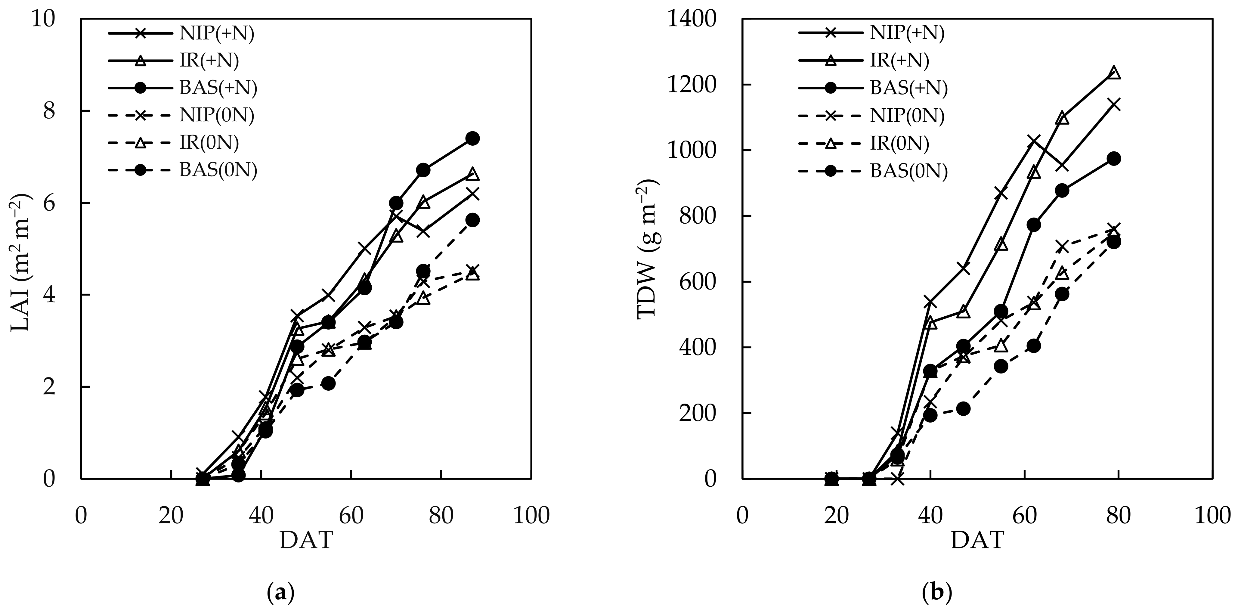
3.5. Temporal Changes in Time-Series Estimation

By changing the survey frequency from two weekly intervals in 2018 to weekly intervals in 2019, our approach could gather a multi-temporal dataset that provided detailed changes in LAI and biomass growth dynamics under field as shown in Figure 12. LAI development increased sharply between 20 June and 10 July after which a steadier growth pattern was observed (Figure 12a). A similar tendency was observed in biomass increase but the increase was prominent in Nipponbare and IR64 under + N conditions (Figure 12b). The weekly observation revealed the detailed growth pattern of the cultivars relative to the growth environment which may not have been revealed by prolonged intervals between monitoring periods This approach helps in real-time monitoring of crop growth at important phenological stages essential for precision agriculture [63], in contrast to single date measurements, which may hinder growth dynamics monitoring in real time [55]. In addition, the hassle of in situ destructive growth evaluation was eliminated [64]. Biomass production in rice is very important for yield formation, and it was pointed out that its importance changes dynamically depending on the growth stage [65]. Therefore, the ability to monitor growth on a fine temporal scale can be used to predict yield with high accuracy.

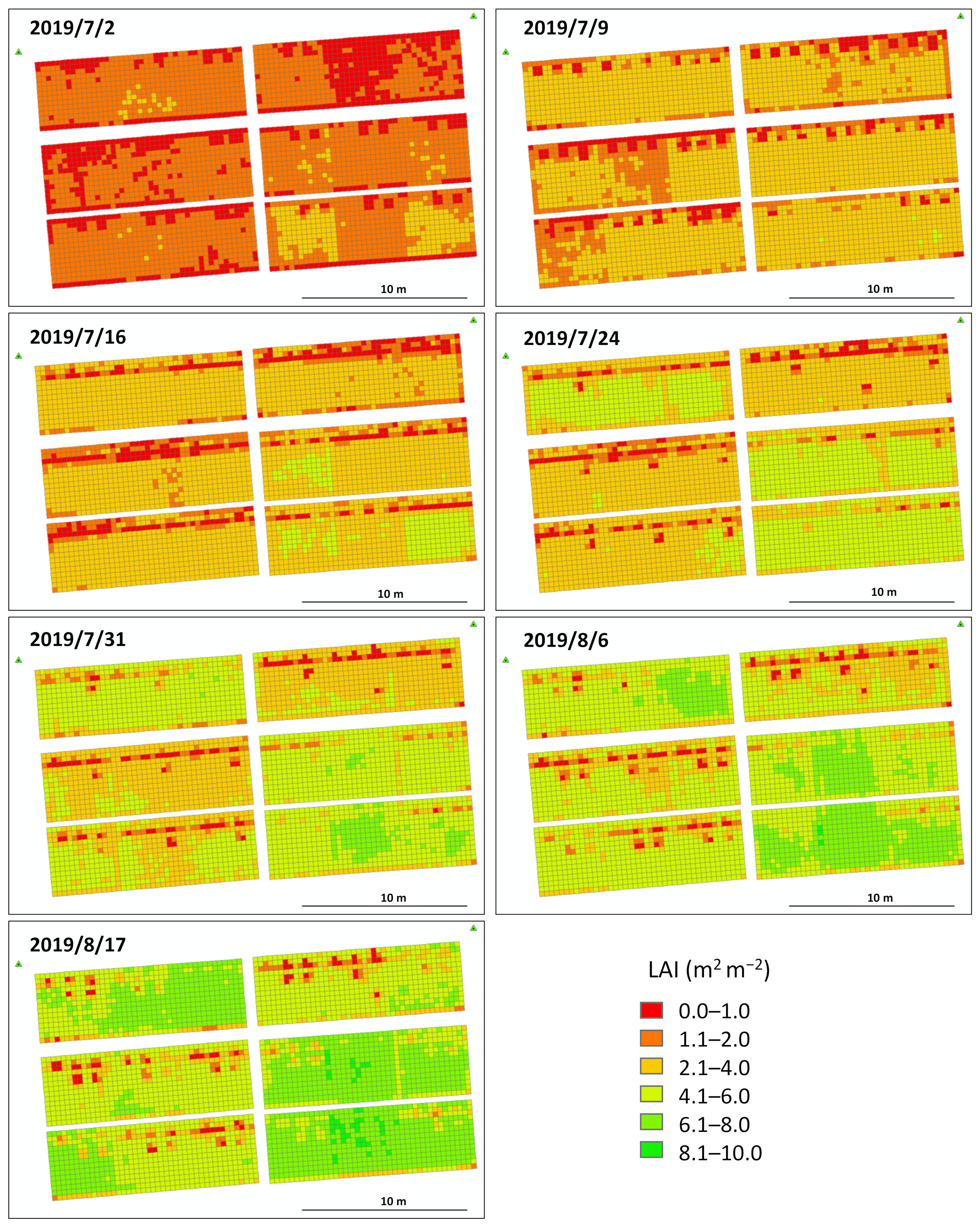
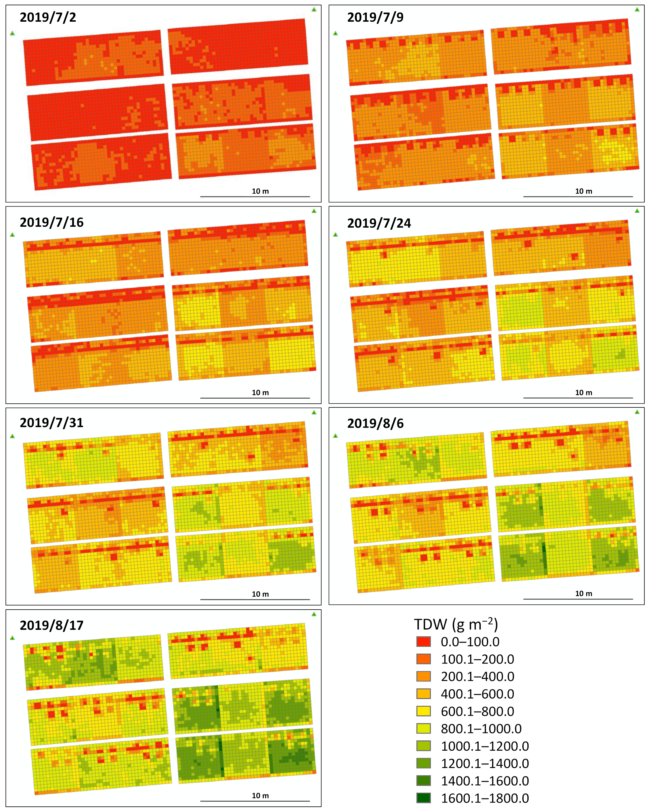
3.6. Spatial Estimation of Biomass Growth

For farmers and researchers alike, information on within-field variations and discrepancies in crop status and edaphic factors is beneficial for making management decisions [66]. In this regard, UAV-based DSM offers clear advantages over conventional manual practices in addition to providing reliable estimates of canopy heights from mean CSM, as seen in this study. Such time saving and real-time monitoring of spatial variations within the field (Figure 13 and Figure 14) can also provide cost-effective and site-specific information for important farm operations, such as fertilizer and pesticide application [67,68,69].

The spatial estimation showed a uniform growth pattern in LAI and TDW at the initial growth stages; however, detailed genotypic differences were evident at the advanced growth stages, with fertilized areas showing more prominent growth. Based on these results, it can be inferred that a good correlation between the variables translates into areas with high canopy height (greener areas), indicating high LAI and aboveground biomass. Thus, this technology can be used to evaluate rice growth spatially. In addition, the technology can be applied not only to precision agriculture technologies, such as site-specific fertilization but also for accurate prediction of growth dynamics in the entire field. The key limitations of the models developed in this study were the effects of weather and genotypic differences between varieties. When the model was applied in 2019, a tendency of overestimation due to reduced sunshine hours during the initial stages of the growing season was observed. As the bad weather persisted, the relationship between plant height, LAI and TDW was affected. Therefore, further investigation is required to understand the variations in the measured and estimated values and to improve the robustness of the model because the genotypes, environmental conditions and parameters investigated in this study were limited.

4. Conclusions

In this study, CSM was used to determine canopy height from UAV aerial images of three rice cultivars in a time series. Manual measurement of relevant growth parameters was performed to validate the UAV aerial surveys. Linear regression models based on the findings of this experiment were established and were used to estimate the biomass of rice plants based on multitemporal and multispectral evaluations. From the observations of the calibration datasets (replications 1 and 3), a strong linear correlation between plant height, LAI and TDW were observed.

A linear relationship with different slopes was obtained for Nipponbare and IR64 combined, and Basmati 370. The estimation model developed using these relational expressions was then applied to the validation dataset (replication 2). Genotypic and environmental differences affected the development of LAI and TDW. In addition, spatial variations in plant growth within the field was observed. The estimation accuracy of the model was found to be high, with relative RMSEs of 20.8% and 28.7% for LAI and TDW, respectively. From this, it was determined that it is possible to perform time-series biomass estimation using this model.

Furthermore, since DSM was used in this study, the influence of weather was relatively small and stable, and easy weekly observations could be made. The results outlined in this study require further investigation in different environmental conditions over multiple years to ascertain its transferability, because several other factors that influence model development and application were not investigated in this study. Furthermore, the spatial resolution of the data can also influence the results obtained, especially in the earlier stages of the growth cycle. By comparing the results under different environmental conditions or planting seasons, we can understand the effect of weather variables such as sunshine, temperature and cloud cover on the application of the model.

References

1. Guo, G.; Wen, Q.; Zhu, J. The Impact of Aging Agricultural Labor Population on Farmland Output: From the Perspective of Farmer Preferences. Math. Probl. Eng. 2015, 2015, 1–7. [Google Scholar] [CrossRef] [Green Version]
2. Gil-Docampo, M.L.; Arza-García, M.; Ortiz-Sanz, J.; Martínez-Rodríguez, S.; Marcos-Robles, J.L.; Sánchez-Sastre, L.F. Above-ground biomass estimation of arable crops using UAV-based SfM photogrammetry. Geocarto Int. 2019, 35, 687–699. [Google Scholar] [CrossRef]
3. Tang, Y.; Chen, M.; Wang, C.; Luo, L.; Li, J.; Lian, G.; Zou, X. Recognition and Localization Methods for Vision-Based Fruit Picking Robots: A Review. Front. Plant Sci. 2020, 11, 510. [Google Scholar] [CrossRef] [PubMed]
4. Li, W.; Niu, Z.; Huang, N.; Wang, C.; Gao, S.; Wu, C. Airborne LiDAR technique for estimating biomass components of maize: A case study in Zhangye City, Northwest China. Ecol. Indic. 2015, 57, 486–496. [Google Scholar] [CrossRef]
5. Jimenez-Berni, J.A.; Deery, D.M.; Rozas-Larraondo, P.; Condon, A.; Rebetzke, G.; James, R.A.; Bovill, W.; Furbank, R.T.; Sirault, X.R.R. High Throughput Determination of Plant Height, Ground Cover, and Above-Ground Biomass in Wheat with LiDAR. Front. Plant Sci. 2018, 9, 237. [Google Scholar] [CrossRef] [PubMed] [Green Version]
6. Macdonald, R.B. A summary of the history of the development of automated remote sensing for agricultural applications. IEEE Trans. Geosci. Remote Sens. 1984, GE-22, 473–482. [Google Scholar]
7. Matese, A.; Toscano, P.; Di Gennaro, S.F.; Genesio, L.; Vaccari, F.P.; Primicerio, J.; Belli, C.; Zaldei, A.; Bianconi, R.; Gioli, B. Intercomparison of UAV, Aircraft and Satellite Remote Sensing Platforms for Precision Viticulture. Remote Sens. 2015, 7, 2971–2990. [Google Scholar] [CrossRef] [Green Version]
8. Cen, H.; Wan, L.; Zhu, J.; Li, Y.; Li, X.; Zhu, Y.; Weng, H.; Wu, W.; Yin, W.; Xu, C.; et al. Dynamic monitoring of biomass of rice under different nitrogen treatments using a lightweight UAV with dual image-frame snapshot cameras. Plant Methods 2019, 15, 32. [Google Scholar] [CrossRef]
9. Hegarty-Craver, M.; Polly, J.; O’Neil, M.; Ujeneza, N.; Rineer, J.; Beach, R.H.; Lapidus, D.; Temple, D.S. Remote Crop Mapping at Scale: Using Satellite Imagery and UAV-Acquired Data as Ground Truth. Remote Sens. 2020, 12, 1984. [Google Scholar] [CrossRef]
10. Burkart, A.; Hecht, V.L.; Kraska, T.; Rascher, U. Phenological analysis of unmanned aerial vehicle based time series of barley imagery with high temporal resolution. Precis. Agric. 2018, 19, 134–146. [Google Scholar] [CrossRef]
11. Candiago, S.; Remondino, F.; De Giglio, M.; Dubbini, M.; Gattelli, M. Evaluating Multispectral Images and Vegetation Indices for Precision Farming Applications from UAV Images. Remote Sens. 2015, 7, 4026–4047. [Google Scholar] [CrossRef] [Green Version]
12. Zhang, C.; Kovacs, J.M. The application of small unmanned aerial systems for precision agriculture: A review. Precis. Agric. 2012, 13, 693–712. [Google Scholar] [CrossRef]
13. George, E.A.; Tiwari, G.; Yadav, R.N.; Peters, E.; Sadana, S. UAV systems for parameter identification in agriculture. In Proceedings of the 2013 IEEE Global Humanitarian Technology Conference: South Asia Satellite (GHTC-SAS), Kerala, India, 23–24 August 2013; pp. 270–273. [Google Scholar]
14. Zhou, X.; Zheng, H.; Xu, X.; He, J.; Ge, X.; Yao, X.; Cheng, T.; Zhu, Y.; Cao, W.; Tian, Y. Predicting grain yield in rice using multi-temporal vegetation indices from UAV-based multispectral and digital imagery. ISPRS J. Photogramm. Remote Sens. 2017, 130, 246–255. [Google Scholar] [CrossRef]
15. Bendig, J.; Yu, K.; Aasen, H.; Bolten, A.; Bennertz, S.; Broscheit, J.; Gnyp, M.L.; Bareth, G. Combining UAV-based plant height from crop surface models, visible, and near infrared vegetation indices for biomass monitoring in barley. Int. J. Appl. Earth Obs. Geoinf. 2015, 39, 79–87. [Google Scholar] [CrossRef]
16. Debell, L.; Anderson, K.; Brazier, R.; King, N.; Jones, L. Water resource management at catchment scales using lightweight UAVs: Current capabilities and future perspectives. J. Unmanned Veh. Syst. 2016, 4, 7–30. [Google Scholar] [CrossRef]
17. Anderson, K.; Gaston, K.J. Lightweight unmanned aerial vehicles will revolutionize spatial ecology. Front. Ecol. Environ. 2013, 11, 138–146. [Google Scholar] [CrossRef] [Green Version]
18. Rasmussen, J.; Ntakos, G.; Nielsen, J.; Svensgaard, J.; Poulsen, R.N.; Christensen, S. Are vegetation indices derived from consumer-grade cameras mounted on UAVs sufficiently reliable for assessing experimental plots? Eur. J. Agron. 2016, 74, 75–92. [Google Scholar] [CrossRef]
19. Honkavaara, E.; Saari, H.; Kaivosoja, J.; Pölönen, I.; Hakala, T.; Litkey, P.; Mäkynen, J.; Pesonen, L. Processing and Assessment of Spectrometric, Stereoscopic Imagery Collected Using a Lightweight UAV Spectral Camera for Precision Agriculture. Remote Sens. 2013, 5, 5006–5039. [Google Scholar] [CrossRef] [Green Version]
20. Lee, K.-J.; Lee, B.-W. Estimation of rice growth and nitrogen nutrition status using color digital camera image analysis. Eur. J. Agron. 2013, 48, 57–65. [Google Scholar] [CrossRef]
21. Christopher, J.T.; Christopher, M.J.; Borrell, A.K.; Fletcher, S.; Chenu, K. Stay-green traits to improve wheat adaptation in well-watered and water-limited environments. J. Exp. Bot. 2016, 67, 5159–5172. [Google Scholar] [CrossRef] [Green Version]
22. Hoffmeister, D.; Bolten, A.; Curdt, C.; Waldhoff, G.; Bareth, G. High-resolution Crop Surface Models (CSM) and Crop Volume Models (CVM) on field level by terrestrial laser scanning. In Proceedings of the Sixth International Symposium on Digital Earth: Models, Algorithms, and Virtual Reality, Beijing, China, 9–12 September 2009. [Google Scholar]
23. Fischer, M.; Huss, M.; Kummert, M.; Hoelzle, M. Use of an ultra-long-range terrestrial laser scanner to monitor the mass balance of very small glaciers in the Swiss Alps. Cryosphere Discuss. 2016, 1, 1–27. [Google Scholar]
24. Barrand, N.E.; Murray, T.; James, T.D.; Barr, S.; Mills, J.P. Optimizing photogrammetric DEMs for glacier volume change assessment using laser-scanning derived ground-control points. J. Glaciol. 2009, 55, 106–116. [Google Scholar] [CrossRef] [Green Version]
25. Baltsavias, E.P.; Favey, E.; Bauder, A.; Bosch, H.; Pateraki, M. Digital Surface Modelling by Airborne Laser Scanning and Digital Photogrammetry for Glacier Monitoring. Photogramm. Rec. 2001, 17, 243–273. [Google Scholar] [CrossRef] [Green Version]
26. Javernick, L.; Brasington, J.; Caruso, B. Modeling the topography of shallow braided rivers using Structure-from-Motion photogrammetry. Geomorphology 2014, 213, 166–182. [Google Scholar] [CrossRef]
27. Verhoeven, G. Taking computer vision aloft—Archaeological three-dimensional reconstructions from aerial photographs with photoscan. Archaeol. Prospect. 2011, 18, 67–73. [Google Scholar] [CrossRef]
28. Geipel, J.; Link, J.; Claupein, W. Combined Spectral and Spatial Modeling of Corn Yield Based on Aerial Images and Crop Surface Models Acquired with an Unmanned Aircraft System. Remote Sens. 2014, 6, 10335–10355. [Google Scholar] [CrossRef] [Green Version]
29. Schirrmann, M.; Giebel, A.; Gleiniger, F.; Pflanz, M.; Lentschke, J.; Dammer, K.-H. Monitoring Agronomic Parameters of Winter Wheat Crops with Low-Cost UAV Imagery. Remote Sens. 2016, 8, 706. [Google Scholar] [CrossRef] [Green Version]
30. Bendig, J.; Bolten, A.; Bennertz, S.; Broscheit, J.; Eichfuss, S.; Bareth, G. Estimating Biomass of Barley Using Crop Surface Models (CSMs) Derived from UAV-Based RGB Imaging. Remote Sens. 2014, 6, 10395–10412. [Google Scholar] [CrossRef] [Green Version]
31. Papadavid, G.; Hadjimitsis, D.; Toulios, L.; Michaelides, S. Mapping potato crop height and leaf area index through vegetation indices using remote sensing in Cyprus. J. Appl. Remote Sens. 2011, 5, 053526. [Google Scholar] [CrossRef]
32. Verhoeven, G.; Vermeulen, F. Engaging with the Canopy—Multi-Dimensional Vegetation Mark Visualisation Using Archived Aerial Images. Remote Sens. 2016, 8, 752. [Google Scholar] [CrossRef] [Green Version]
33. Freeman, K.W.; Girma, K.; Arnall, D.B.; Mullen, R.W.; Martin, K.L.; Teal, R.K.; Raun, W.R. By-Plant Prediction of Corn Forage Biomass and Nitrogen Uptake at Various Growth Stages Using Remote Sensing and Plant Height. Agron. J. 2007, 99, 530–536. [Google Scholar] [CrossRef] [Green Version]
34. Sharma, L.K.; Bu, H.; Franzen, D.W.; Denton, A. Use of corn height measured with an acoustic sensor improves yield estimation with ground based active optical sensors. Comput. Electron. Agric. 2016, 124, 254–262. [Google Scholar] [CrossRef] [Green Version]
35. Rock, G.; Ries, J.B.; Udelhoven, T. Sensitivity analysis of UAV-photogrammetry for creating digital elevation models (DEM). In Proceedings of the International Archives of the Photogrammetry, Remote Sensing and Spatial Information Sciences, Zurich, Switzerland, 14–16 September 2011; pp. 1–5. [Google Scholar]
36. Tahar, K.N.; Tahar, K.N.; Ahmad, A.; Abdul, W.; Wan, A.; Akib, M.; Mohd, W.; Mohd, N.W. Assessment on Ground Control Points in Unmanned Aerial System Image Processing for Slope Mapping Studies. Int. J. Sci. Eng. Res. 2012, 3, 1–10. [Google Scholar]
37. Nouwakpo, S.K.; Weltz, M.A.; McGwire, K.C. Assessing the performance of structure-from-motion photogrammetry and terrestrial LiDAR for reconstructing soil surface microtopography of naturally vegetated plots. Earth Surf. Process. Landf. 2016, 41, 308–322. [Google Scholar] [CrossRef]
38. Japan Meteorological Agency: Search Past Weather Data. Available online: http://www.data.jma.go.jp/obd/stats/etrn/view/-nml_amd_ym.php?prec_no=44&block_no=1133&year=&month=&day=&view (accessed on 23 March 2021).
39. Matsumoto, T.; Wu, J.; Kanamori, H.; Katayose, Y.; Fujisawa, M.; Namiki, N.; Mizuno, H.; Yamamoto, K.; Antonio, B.A.; Baba, T.; et al. The map-based sequence of the rice genome. Nature 2005, 436, 793–800. [Google Scholar]
40. Mackill, D.J.; Khush, G.S. IR64: A high-quality and high-yielding mega variety. Rice 2018, 11, 1–11. [Google Scholar] [CrossRef] [Green Version]
41. Mojulat, W.C.; Yusop, M.R.; Ismail, M.R.; Juraimi, A.S.; Harun, A.R.; Ahmed, F.; Tanweer, F.A.; Latif, A. Analysis of Simple Sequence Repeat Markers Linked to Submergence Tolerance on Newly Developed Rice Lines Derived from MR263 × Swarna-Sub1. Sains Malays. 2017, 46, 521–528. [Google Scholar]
42. Peng, S.; Khush, G.S. Four Decades of Breeding for Varietal Improvement of Irrigated Lowland Rice in the International Rice Research Institute. Plant Prod. Sci. 2003, 6, 157–164. [Google Scholar] [CrossRef]
43. San-oh, Y.; Mano, Y.; Ookawa, T.; Hirasawa, T. Comparison of dry matter production and associated characteristics between direct-sown and transplanted rice plants in a submerged paddy field and relationships to planting patterns. Field Crop. Res. 2004, 87, 43–58. [Google Scholar] [CrossRef]
44. Gindraux, S.; Boesch, R.; Farinotti, D. Accuracy Assessment of Digital Surface Models from Unmanned Aerial Vehicles’ Imagery on Glaciers. Remote Sens. 2017, 9, 186. [Google Scholar] [CrossRef] [Green Version]
45. Yamaguchi, T.; Tanaka, Y.; Imachi, Y.; Yamashita, M.; Katsura, K. Feasibility of Combining Deep Learning and RGB Images Obtained by Unmanned Aerial Vehicle for Leaf Area Index Estimation in Rice. Remote Sens. 2020, 13, 84. [Google Scholar] [CrossRef]
46. Van Iersel, W.; Straatsma, M.; Addink, E.; Middelkoop, H. Monitoring height and greenness of non-woody floodplain vegetation with UAV time series. ISPRS J. Photogramm. Remote Sens. 2018, 141, 112–123. [Google Scholar] [CrossRef]
47. Fageria, N.K. Yield Physiology of Rice. J. Plant Nutr. 2007, 30, 843–879. [Google Scholar] [CrossRef]
48. Yoshida, H.; Horie, T.; Katsura, K.; Shiraiwa, T. A model explaining genotypic and environmental variation in leaf area development of rice based on biomass growth and leaf N accumulation. Field Crop. Res. 2007, 102, 228–238. [Google Scholar] [CrossRef]
49. Njinju, S.M.; Samejima, H.; Katsura, K.; Kikuta, M.; Gweyi-Onyango, J.P.; Kimani, J.M.; Yamauchi, A.; Makihara, D. Grain yield responses of lowland rice varieties to increased amount of nitrogen fertilizer under tropical highland conditions in central Kenya. Plant Prod. Sci. 2018, 21, 59–70. [Google Scholar] [CrossRef]
50. Semchenko, M.; Zobel, K. The effect of breeding on allometry and phenotypic plasticity in four varieties of oat (Avena sativa L.). Field Crop. Res. 2005, 93, 151–168. [Google Scholar] [CrossRef]
51. Yoshida, H.; Horie, T. A model for simulating plant N accumulation, growth and yield of diverse rice genotypes grown under different soil and climatic conditions. Field Crop. Res. 2010, 117, 122–130. [Google Scholar] [CrossRef]
52. Koppe, W.; Gnyp, M.L.; Hütt, C.; Yao, Y.; Miao, Y.; Chen, X.; Bareth, G. Rice monitoring with multi-temporal and dual-polarimetric terrasar-X data. Int. J. Appl. Earth Obs. Geoinf. 2012, 21, 568–576. [Google Scholar] [CrossRef]
53. Lopez-Sanchez, J.M.; Ballester-Berman, J.D.; Hajnsek, I.; Hajnsek, I. First Results of Rice Monitoring Practices in Spain by Means of Time Series of TerraSAR-X Dual-Pol Images. IEEE J. Sel. Top. Appl. Earth Obs. Remote Sens. 2011, 4, 412–422. [Google Scholar] [CrossRef]
54. Ribbes, F.; Letoan, T. Rice field mapping and monitoring with radarsat data. Int. J. Remote Sens. 1999, 20, 745–765. [Google Scholar] [CrossRef]
55. Kawamura, K.; Asai, H.; Yasuda, T.; Khanthavong, P.; Soisouvanh, P.; Phongchanmixay, S. Field phenotyping of plant height in an upland rice field in Laos using low-cost small unmanned aerial vehicles (UAVs). Plant Prod. Sci. 2020, 23, 452–465. [Google Scholar] [CrossRef]
56. Willkomm, M.; Bolten, A.; Bareth, G. Non-destructive monitoring of rice by hyperspectral in-field spectometry and UAV-based remote sensing; Case study of field-grown rice in North Rhine-Westphalia, Germany. Int. Arch. Photogramm. Remote Sens. Spat. Inf. Sci. 2016, XLI-B1, 12–19. [Google Scholar] [CrossRef] [Green Version]
57. Aasen, H.; Burkart, A.; Bolten, A.; Bareth, G. Generating 3D hyperspectral information with lightweight UAV snapshot cameras for vegetation monitoring: From camera calibration to quality assurance. ISPRS J. Photogramm. Remote Sens. 2015, 108, 245–259. [Google Scholar] [CrossRef]
58. Ehlert, D.; Adamek, R.; Horn, H.-J. Laser rangefinder-based measuring of crop biomass under field conditions. Precis. Agric. 2009, 10, 395–408. [Google Scholar] [CrossRef]
59. Fang, H.; Li, W.; Wei, S.; Jiang, C. Seasonal variation of leaf area index (LAI) over paddy rice fields in NE China: Inter-comparison of destructive sampling, LAI-2200, digital hemispherical photography (DHP), and AccuPAR methods. Agric. For. Meteorol. 2014, 198, 126–141. [Google Scholar] [CrossRef]
60. Pierson, E.A.; Mack, R.N.; Black, R.A. The effect of shading on photosynthesis, growth, and regrowth following defoliation for Bromus tectorum. Oecologia 1990, 84, 534–543. [Google Scholar] [CrossRef]
61. Song, L.; Jin, J. Effects of Sunshine Hours and Daily Maximum Temperature Declines and Cultivar Replacements on Maize Growth and Yields. Agronomy 2020, 10, 1862. [Google Scholar] [CrossRef]
62. Zhang, T.; Huang, Y.; Yang, X. Climate warming over the past three decades has shortened rice growth duration in China and cultivar shifts have further accelerated the process for late rice. Glob. Chang. Biol. 2013, 19, 563–570. [Google Scholar] [CrossRef]
63. Hansen, P.; Schjoerring, J. Reflectance measurement of canopy biomass and nitrogen status in wheat crops using normalized difference vegetation indices and partial least squares regression. Remote Sens. Environ. 2003, 86, 542–553. [Google Scholar] [CrossRef]
64. Jay, S.; Rabatel, G.; Hadoux, X.; Moura, D.; Gorretta, N. In-field crop row phenotyping from 3D modeling performed using Structure from Motion. Comput. Electron. Agric. 2015, 110, 70–77. [Google Scholar] [CrossRef] [Green Version]
65. Takai, T.; Matsuura, S.; Nishio, T.; Ohsumi, A.; Shiraiwa, T.; Horie, T. Rice yield potential is closely related to crop growth rate during late reproductive period. Field Crop. Res. 2006, 96, 328–335. [Google Scholar] [CrossRef]
66. Maes, W.H.; Steppe, K. Perspectives for Remote Sensing with Unmanned Aerial Vehicles in Precision Agriculture. Trends Plant Sci. 2019, 24, 152–164. [Google Scholar] [CrossRef]
67. Portz, G.; Molin, J.P.; Jasper, J. Active crop sensor to detect variability of nitrogen supply and biomass on sugarcane fields. Precis. Agric. 2011, 13, 33–44. [Google Scholar] [CrossRef]
68. Dammer, K.H.; Wartenberg, G. Sensor-based weed detection and application of variable herbicide rates in real time. Crop Prot. 2007, 26, 270–277. [Google Scholar] [CrossRef]
69. Shanahan, J.; Kitchen, N.; Raun, W.; Schepers, J. Responsive in-season nitrogen management for cereals. Comput. Electron. Agric. 2008, 61, 51–62. [Google Scholar] [CrossRef] [Green Version]
Figure 1. Study fields and layouts in 2018 and 2019.
Remotesensing 13 02388 g001
Figure 2. Examples of photos of 8 hills of 3 cultivars (Nipponbare, IR64 and Basmati370) with medium fertilization in replication 2 taken on (a) 3 July and (b) 27 July in 2018.
Remotesensing 13 02388 g002
Figure 3. The flowchart of generation of the digital surface model and ortho mosaic image from UAV images.
Remotesensing 13 02388 g003
Figure 4. Procedures of spatio-temporal estimations using canopy surface models.
Remotesensing 13 02388 g004
Figure 5. Comparison of seasonal changes in crop growth; (a,d) LAI, (b,e) TDW and (c,f) PL at various days after transplanting (DAT) in 2018 and 2019 for three rice cultivars: Basmati370 (BAS), IR64 (IR) and Nipponbare (NIP).
Remotesensing 13 02388 g005
Figure 6. Examples of canopy surface model (CSM) for three rice cultivars in two vegetation seasons.
Remotesensing 13 02388 g006
Figure 7. Comparison between; (a) measured plant length (PL) and two types of canopy heights (CH) calculated from the mean values and 97th percentile of CSMn and (b) the seasonal relationships between them.
Remotesensing 13 02388 g007
Figure 8. Canopy height calculation from (a) ortho image and (b) CSM in a 30 × 30 cm area covering two plants.
Remotesensing 13 02388 g008
Figure 9. Relationship of (a) Leaf area index (LAI) and (b) aboveground biomass dry weight (TDW) with measured plant height in 2018 (Rep. 1 and 3).
Remotesensing 13 02388 g009
Figure 10. Accuracy assessment of CSM derived estimated (a) LAI and (b) TDW against standard ground-based measurements in 2018 (Rep. 2). BAS: n = 12, NIP and IR: n = 24.
Remotesensing 13 02388 g010
Figure 11. Relationship between the estimated and observed values of (a) TDW and (b) LAI in 2019 (Rep. 1, 2 and 3). BAS: n = 24, NIP and IR: n = 48.
Remotesensing 13 02388 g011
Figure 12. Observed temporal changes of estimated (a) LAI and (b) TDW in 2019 (Rep. 2) at various days after transplanting (DAT).
Remotesensing 13 02388 g012
Figure 13. Examples of Spatial estimation of LAI in 2019 using the DSM model (greener areas represent higher LAI).
Remotesensing 13 02388 g013
Figure 14. Example of spatial estimation of TDW in 2019 using the DSM model (greener areas represent higher biomass growth).
Remotesensing 13 02388 g014