Article

Estimation of the Monthly Dynamics of Surface Water in Wetlands from Satellite and Secondary Hydro-Climatological Data

by
Antonio-Juan Collados-Lara
1,*,
Eulogio Pardo-Igúzquiza
2,
David Pulido-Velazquez
1 and
Leticia Baena-Ruiz
1
1
Instituto Geológico y Minero de España (IGME, CSIC), Urb. Alcázar del Genil, 4. Edificio Zulema Bajo, 18006 Granada, Spain
2
Instituto Geológico y Minero de España (IGME, CSIC), Ríos Rosas, 23, 28003 Madrid, Spain
*
Author to whom correspondence should be addressed.
Remote Sens. 2021, 13(12), 2380; https://doi.org/10.3390/rs13122380
Submission received: 27 April 2021 / Revised: 15 June 2021 / Accepted: 15 June 2021 / Published: 18 June 2021

Abstract

:
Satellites produce valuable information for studying the surface water in wetlands, but in many cases the period covered, the spatial resolution and/or the revisit frequency is not enough to produce long historical series. In this paper we propose a novel method which uses regression models that include climatic and hydrological variables to complete the satellite information. We used this method in the Lagunas de Ruidera wetland (Spain). We approached the monthly dynamic of the surface water for a long period (1984–2015). Information from LANDSAT (30-m resolution) and MODIS (250-m resolution) satellites were tested but, due to the size of some lagoons, only the LANDSAT approach produced satisfactory results. An ensemble of regression models based on hydro-climatological explanatory variables was defined to complete the gaps in the monthly surface water. It showed a root mean squared error of around 476 pixels (0.4 Km2) in the cross-validation analysis. Our analysis showed that the explanatory variables with a more significant participation in the regression ensemble are the aquifer discharge, the effective precipitation and the surface water from the previous month. From January to June, the mean surface water in Lagunas de Ruidera is around 4.3 Km2. In summer a reduction of around 13% of the surface water can be observed, which is recovered during the autumn.

1. Introduction

Satellite images provide useful information for monitoring some climatic and hydrological variables with different spatial resolutions and revisit frequencies. For example, they provide information about water [1,2], area covered by snow [3,4], different land uses [5] in water resource systems and urban physical characteristics [6]. This paper focuses on the analyses of wetland surface-water mapping.
Wetlands are systems with significant environmental value. In accordance with the Ramsar convention [7], they can be used to improve water quality, store floodwater, maintain surface water during dry periods and provide valuable habitats for wildlife. They can also help to regulate urban temperature [8] and have a significant recreational and tourism interest supporting multiple ecosystem services [9]. The Ramsar convention is an intergovernmental convention that provides the framework for national action and international co-operation for the conservation and wise use of wetlands and their resources. It was signed in the Iranian city of Ramsar in 1971 and came into force in 1975. It also defines a list of wetlands of international interest and has the aim of defining a framework for their conservation. Note that the Convention uses a broad definition of wetlands (lakes and rivers, underground aquifers, swamps and marshes, wet grasslands, peatlands, oases, estuaries, deltas and tidal flats, mangroves and other coastal areas, coral reefs, and all human-made sites such as fish ponds, rice paddies, reservoirs and salt pans).
Wetland dynamics can be very sensitive to climate conditions and anthropogenic impact [10,11]. For example, in coastal areas, they can be affected by sea water intrusion [12,13]. In general, in accordance with the potential future climate scenarios [14], this impact on water resource systems will be exacerbated in the future due to both climate [15] and global change [16]. Adaptation strategies will be required to reduce the future potential impact in order to define sustainable management measures [17,18].
From a methodological point of view, the problems related with surface water mapping algorithms from surface reflectance satellite data have been previously resolved by using different water-related spectral indices and sensors [1,2]. The spatial resolution and the revisit frequency depend on the satellite data, (e.g., SENTINEL-2 has a spatial resolution of 10 m and a revisit frequency of 10 days [19], LANDSAT has a spatial resolution of 30 m and a revisit frequency of 16 days [20], and MODIS 250 m spatial resolution and daily revisit frequency [21]). In the literature, we can find some studies that have tried to use downscaling MODIS surface reflectance to improve the accuracy of the estimations for these cases [22,23]. The temporal coverage for the satellites with a higher revisit frequency is scarce (e.g., MODIS covers from 2000 and SENTINEL covers from 2015). However, the temporal coverage for some studies (e.g., hydrological applications or land use changes) should be long enough (e.g., 30 years) to be able to carry out an appropriate statistical analysis. The LANDSAT satellite, which has a good spatial resolution (30 m from mission 5), covers from 1984. Therefore LANDSAT has been used in several surface earth applications (water detection [24], snow cover area [25] and land use change [26]). The low revisit frequency of satellite data for land surface variable mapping can be complemented by using other well sampled explanatory variables related to the target variable as we propose in this study.
In the case of wetlands, the amount of water and, therefore, the surface water is related to climatic variables (e.g., precipitation, temperature, evapotranspiration). Wetlands are in general linked to groundwater resources [27] and, therefore, hydrological variables such as the aquifer discharge are closely related to surface water in wetlands. These variables can provide valuable information to complete the data obtained from satellites. Regression models based on different explanatory variables have been used successfully to estimate different climatic and hydrological variables (e.g., precipitation [28], temperature [29], and snow depth and snow water equivalent [30]).
This surface water is a key variable that should be taken into account in the decision making process when assessing sustainable management strategies in water resource systems for wetlands. In order to be able to draw conclusions which are statistically representative of the hydrological dynamic and/or the analyses of management strategies, long enough series covering multiple years should be analysed [31,32]. Most of these hydrological and water resource studies covering long time periods work at a monthly scale [33,34,35].
In this paper, we propose a novel method to approach long monthly series of surface water in small lagoons that require high spatial resolution information. It combines visual satellite data and regression models that include climatic and hydrological explanatory variables to complete the information obtained from the satellite data. The main novelty of this methodology is the use of hydro-climatological information to complete and approach the surface water dynamic observed with the satellite information. It is a general method that can be applied to other wetlands taking into account the dependence of surface water on hydro-climatological information. We applied the proposed methodology to the Ramsar wetland “Lagunas de Ruidera” (Spain) that integrates groundwater-dependent small size lagoons. Some studies were developed in this area for the analyses of different issues such as bacterial and microbial diversity [36,37], but none of them tried to map the surface water within the historical period (1984−2015). Therefore, we analysed a critical problem in this groundwater-dependent Ramsar site. The particularities of our system forced us to also include some novelties in our method of analysis. As the surface water in our wetland is relatively small (between 2.7 and 6.3 km²), in order to identify the surface water with enough spatial detail we had to use satellite images with high spatial resolution (e.g., LANDSAT with a resolution of 30 m). The problem is that the frequency of data is low (around 16 days). We also analysed the MODIS (MOD09GQ) daily surface reflectance data, but their spatial resolution is too low (250 m) to assess the domain of open water in the wetland. Combined use of satellite images with different spatial resolution and the revisit frequency has already been carried out in the study of wetlands in previous research [22,23]. Nevertheless, as far as we know, an integrated analysis of potential explanatory variables has not been carried out in any of them in which, in addition to the satellite images, some climatic (precipitation, temperature and evapotranspiration) and hydrogeological variables (aquifer discharge to the groundwater-dependent lagoons) are included to complete the satellite information. This requires the use of mathematical models to simulate surface water–groundwater interaction [38,39,40] as auxiliary tools to assess discharge, which is an important variable with which to understand and approach the dynamic of groundwater dependent wetlands [41], such as the “Lagunas de Ruidera”.

2. Study Area

The Lagunas de Ruidera wetland area (south-eastern Spain) is a group of small natural lakes and a reservoir (Peñarroya) located in the headwaters of the Guadiana River Basin (Figure 1a), where there is a strong natural interaction between groundwater and surface water. This area also highlights a conflict between groundwater dependent ecosystems and groundwater pumping to supply demands (mainly irrigation demands). The site is critical for the functioning of the regional hydrological system and serves as an important water reservoir in this semi-arid region. The lagoons are located on a plateau formed mainly of limestone and dolomites. The lagoons overflow and flood each other forming waterfalls due to geological formations such as travertine barriers. The system consists of 15 lagoons along a distance of around 35 km. The elevation of the area varies from 750 to 950 m a.s.l. (see Figure 1b) and the difference of elevation between the first lagoon and the reservoir is around 120 m. The mean yearly precipitation in the area in the period 1984-2015 is 477 mm year−1 and the mean temperature is 14.8 °C. The lagoons receive significant groundwater contributions, (mean of 57 Mm3 year−1 for the period 1984–2015). The Lagunas de Ruidera has a significant environmental value with a great diversity of animal and plant species. The site hosts many globally threatened species including the bivalve Unio tumidiformis and the water vole Arvicola sapidus as well as numerous fish and bird species, especially Anatidae. It is also important for the region from an economic point of view, with many tourist activities. The site is also of archaeological and historic significance and is used for traditional agriculture, research and recreational activities. In addition, the water resources from the area are important to the supply of water demands within the region. Due to these characteristics, the zone was classified as a Natural Park (from 1979) and a Ramsar area (from 2011).

3. Methodology and Data

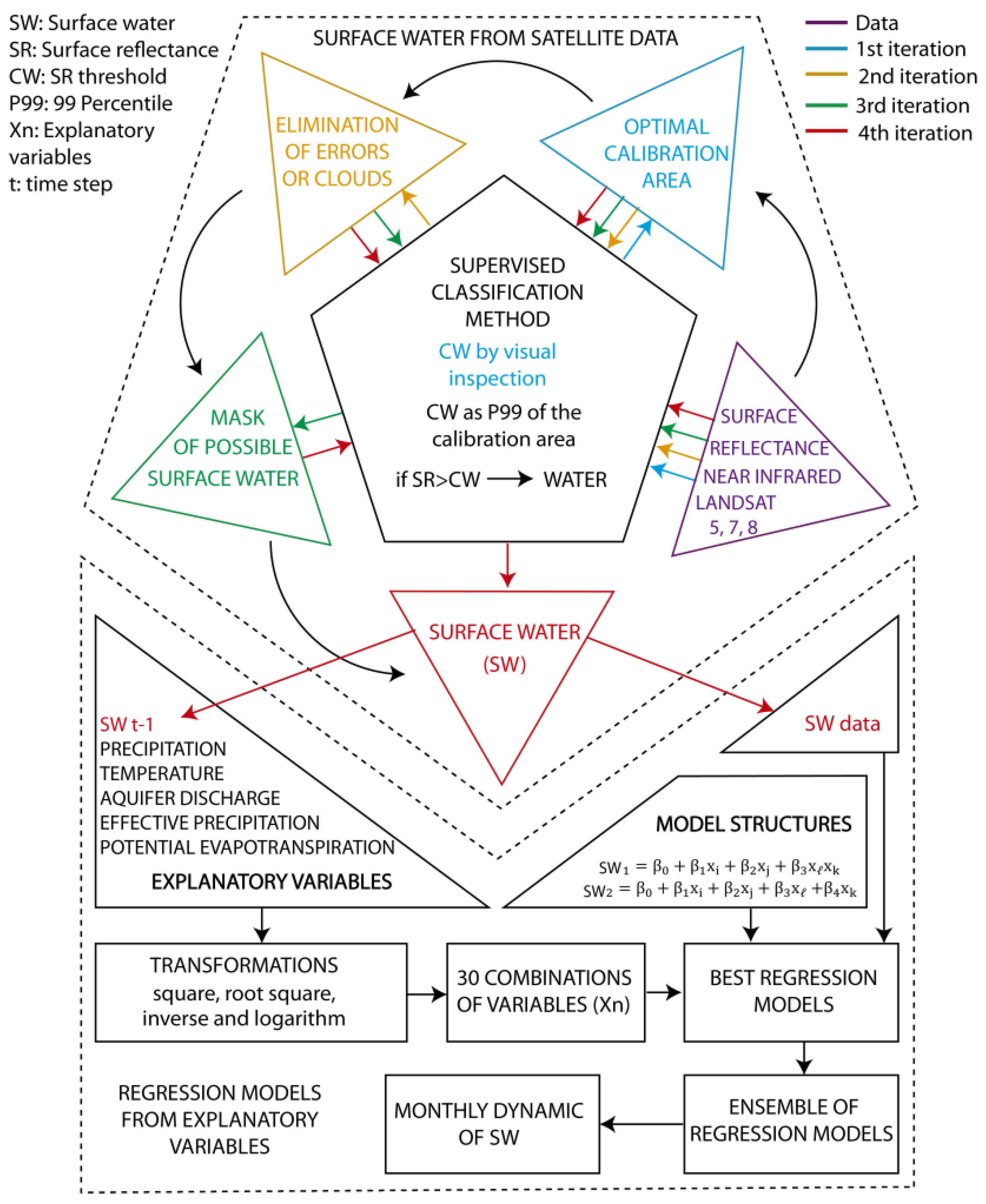
The proposed method (see Figure 2) requires the identification of the surface water using surface reflectance from satellites and to calibrate multiple regression models which complete the available information provided by the satellite data. Both procedures are described below.

3.1. Identification of the Surface Water from Satellite Data

The surface reflectance measures the fraction of incoming solar radiation reflected from Earth’s surface to the satellite sensor. It is useful for the detection and characterisation of the status and changes of the Earth’s surface. We propose using the near infrared band, which can be used for mapping shorelines. The surface water can be identified because it has a low surface reflectance compared to other land cover classes.
For surface water identification we used the supervised classification methodology, which requires selecting representative samples for each land cover class. The algorithm uses the statistics obtained in these training sites for the entire image to identify these cover classes. In our case study, the target cover class is the surface water. We used a threshold of the surface reflectance from satellite, which varies temporally, to identify the surface water. It is obtained from a selected calibration area or training area. A pixel is considered as covered by water if its surface reflectance is below or equal to the threshold defined for the corresponding day. Our methodology, based on this assumption, aims to reduce the errors in the water identification by incorporating the following procedures (see Figure 1):
(a)
Selection of the calibration area
The calibration area is used to define the threshold of surface reflectance that best defines the surface water. As a first approximation we considered a stationary surface reflectance threshold identified visually from some satellite images. We created a map that shows the spatial distribution of the number of times that each pixel is below the considered threshold. The areas with the higher values were considered as potential calibration areas, taking into account that their probability of always being covered by water is high. Note that the calibration area can be composed of different areas or lagoons and the threshold identified visually was only used to define good calibration areas. In our case study the calibration area is composed of two areas that represent the two main surface water characteristics of the case study. We considered 49 pixels of the reservoir next to the dam and 366 pixels of the lagoons. Both of them are always covered by water. This allowed us to take into account the different conditions of surface reflectance of both water bodies (reservoir and natural lagoons), which are related to the different water depths. The maximum depth of the natural lagoons is between 10 and 20 m and in the case of the reservoir it can reach 35 m.
(b)
Elimination of images with errors or clouds
Satellite images have errors and clouds which may prevent the correct identification of water. Three kinds of filters were included to rule out these images with errors and clouds. The first one considers that the calibration areas should have a low surface reflectance because they are covered by water. The second one uses a stationary threshold to identify clouds (high surface reflectance) in the study area, and the last one is a filter based on the minimum and maximum surface water identified in the historical period.
(c)
Creation of a mask of possible surface water
We also created a mask of possible surface water in order to reduce the algorithm errors by constraining the solution to the pixels which are covered by water on at least one day in the study period. The mask was defined by using the proposed algorithm and corrected with the digital elevation model and an aerial photograph.
(d)
Surface water mapping by applying a temporally variable threshold
The threshold for distinguishing surface water was considered as the 99th percentile of the surface reflectance in the calibration areas. Note that these areas are always covered by water during the studied period. The images with errors and clouds were ruled out and the mask was incorporated to reduce the errors.
In this study, only one band, the near infrared band from the different LANDSAT satellite missions, was used for surface water mapping. In fact, despite there being more sophisticated methods for mapping water using multiple spectral bands or multiple sensors [42] the mapping of open surface water, in the area considered in this paper, is a task that can be efficiently performed by using only the near infrared band. This is the case because the spectral signature of water calculated by using the near infrared band is efficient for mapping surface water and it is simply defined as the values that are below a given threshold. Thus, the surface water is identified as the pixels whose digital number, in the near infrared band, is smaller than a calibrated temporary variable threshold. It should be noted that it is the temporal variability of the threshold that allows us to separate water from other surfaces.

3.2. Regression Models from Explanatory Variables

The information obtained at a certain resolution by using satellite data within the selected period is usually incomplete, due to the frequency of satellite data acquisition, the errors in the sensor and the presence of clouds. In this paper we propose using secondary hydro-climatological information to complete the monthly surface water data through regression models calibrated with the available data. The objective is to estimate the monthly surface water area for those months without satellite-based information. The monthly surface water for a given month is calculated as the arithmetic mean of the satellite surface water areas available for that month. It is considered that intra-month variability is negligible with respect to the inter-month variability. Two regression model structures (previously used [3,30] for snow dynamic estimation) were tested:
SW 1 = β 0 + β 1 x i + β 2 x j + β 3 x x k
SW 2 = β 0 + β 1 x i + β 2 x j + β 3 x + β 4 x k
where SW is the monthly surface water to be estimated (1 refers to the first structure and 2 to the second), { x i , x j , x , x k }   are the explanatory variables (including transformations of them), and { β 0 ,   β 1 , β 2 , β 3 , β 4 } are unknown parameters estimated from experimental data.
The explanatory variables used in this study can be divided into three categories:
(a)
Main climatic variables: precipitation and temperature.
(b)
Those derived from the main climatic variables: potential evapotranspiration and effective precipitation.
(c)
Hydrological variables: aquifer discharge and surface water in the previous month.
We also considered their mathematical transformations (square, square root, logarithm and inverse). The indices { x i , x j , x , x k } represent the explanatory variables. Each regression model has four explanatory variables that can be selected from the six considered variables and their transformations.
The regression models were calibrated by applying a maximum likelihood normal regression for both structures and their performance was measured in terms of correlation coefficient (R2). The calibration of the regression models must be carried out using pairs of satellite measurements made in adjacent months, because the surface water in the previous month was used as an explanatory variable. The performance of the obtained models was also tested under different estimation modes by calculating the root mean squared error (RMSE). We used a forecasting mode that only uses the satellite information to define the initial conditions (the first value of the surface water series) for a sequential simulation of the entire monthly series in the selected period. In this forecast model, the estimated surface water in each time step is used as the initial value of surface water in the next time step. The results were also compared with a completion mode that updates the monthly estimate of the surface water with the value deduced from satellite data when it is known. In this case, when measurements from satellite are available, they are used as initial conditions to calculate the surface water in the following month. The completion mode was applied by using different estimation procedures (forward, backward and combined forward–backward). The forward estimation procedure is executed from 1984 to 2015 and the backward procedure is executed from 2015 to 1984. The forward–backward estimation mode is a weighted estimation from the forward and backward approaches, which estimates each time step as a weighted average of both estimation modes. In the forward mode the weights are calculated considering the distance of the target time step to the previous month with available data. In the backward estimation mode, they depend on the distance to the next available month with data.
In our case study several regression models showed similar performance statistics and we opted for using an ensemble of regression models to do the final estimations. It was made up of the six best regression models for each considered regression structure (12 models in total). It allowed us to identify the most significant explanatory variables to estimate the surface water in our case study.

3.3. Data

The methodology was applied to the case study for the period 1984–2015. It requires surface reflectance data from satellite and hydro-climatological data. Two sources of satellite information (LANDSAT and MODIS) were tested for the study domain (Figure 2). In the case of LANDSAT, information from three satellite missions (5, 7, and 8) was used. We used the near infrared bands (band 4 in the case of LANDSAT 5 and 7 and band 5 in the case of LANDSAT 8), which provide useful information to identify shorelines. The spatial resolution of LANDSAT is 30 meters, and the revisit frequency is around 16 days. In the case of the MODIS surface reflectance, we used the product MOD09GQ which provides two bands of surface reflectance at 250 m resolution with daily revisit frequency. For this product we used band 2 which can identify surface water better than band 1 due to its higher wavelength. Note that for the studied period MODIS was only available from 2000 to 2015. With respect the hydro-climatological variables, precipitation and temperature (mean, maximum and minimum) were obtained from the Spain02 (v5) project [43,44]. Potential evapotranspiration and effective precipitation were calculated from temperature by using the Hargraves method [45] at a daily scale. These variables were calculated for the study basin within the study domain (Figure 1). The aquifer discharge was obtained from a Finite Difference groundwater model calibrated with historical data from the period (1974–2010).

4. Results

4.1. Surface Water from Satellite Data

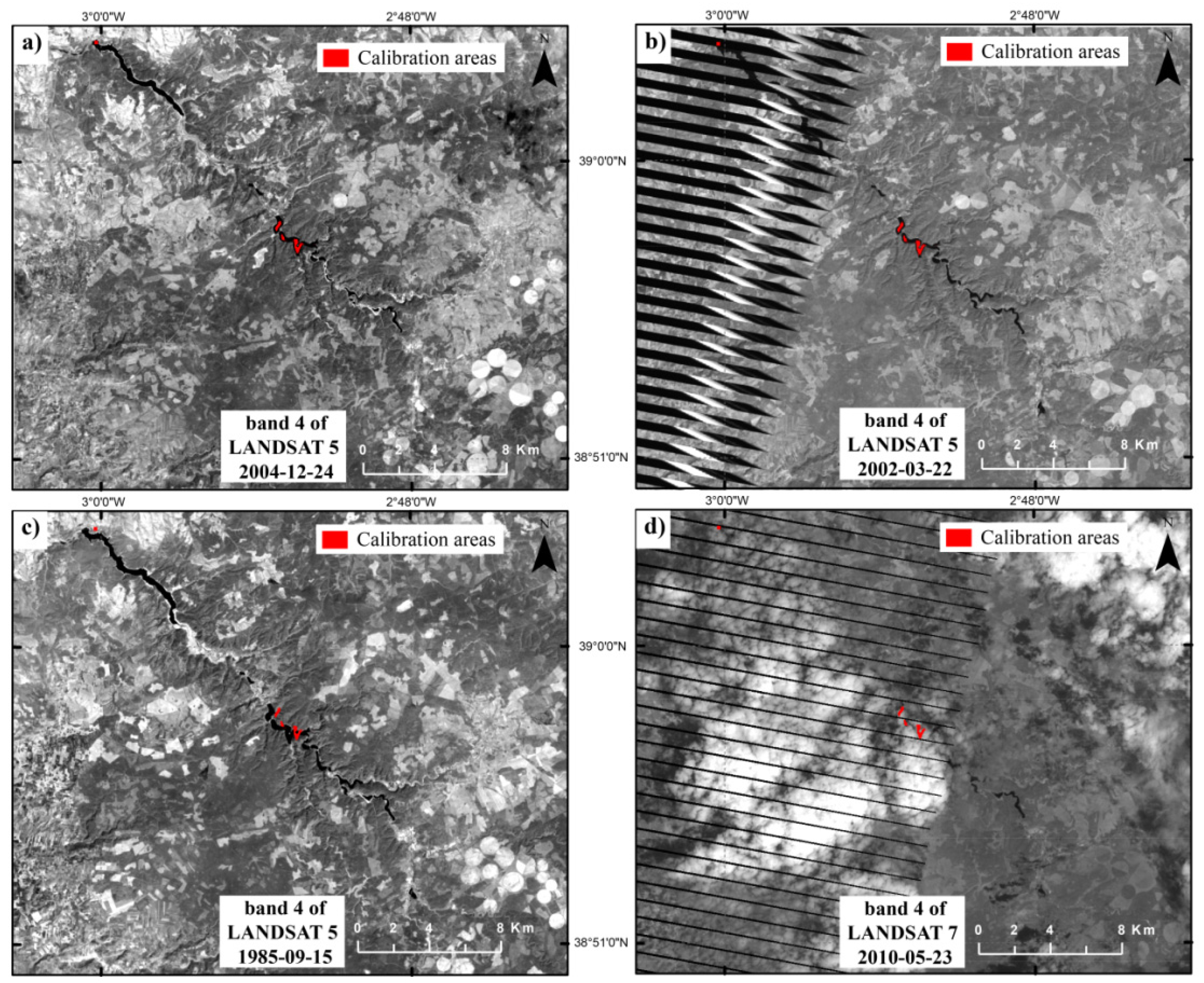
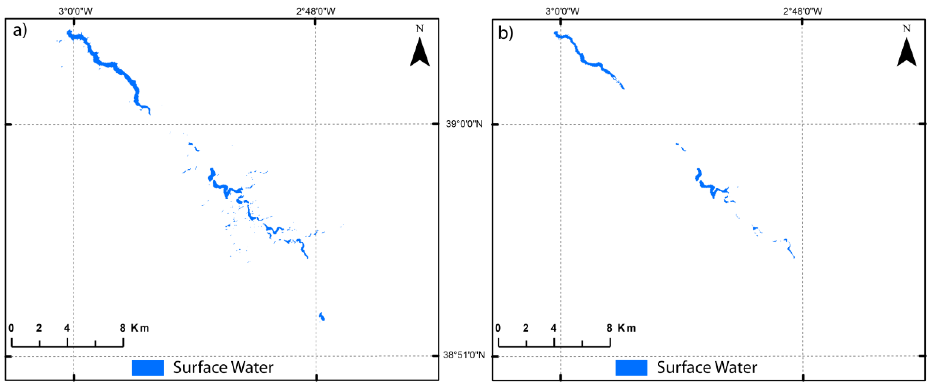
The first satellite source investigated in this study was LANDSAT (30 m resolution). In order to obtain a good calibration area, as first approximation, we used the land surface reflectance provided by the different satellite images to obtain the number of images per pixel that had a low surface reflectance (below a threshold obtained visually from some images). From this map, we considered the calibration area defined by the pixels that have a value higher than 520. Note that the total number of images, considering also those ones with errors and clouds, is 790. This ensures that the calibration area is always covered by water. We also added to the obtained area (366 pixels) 49 pixels of the reservoir to take into account the different conditions of surface reflectance of both water bodies (reservoir and natural lagoons), which are related to the different water depths. These pixels were selected from the part of the reservoir which is always covered by water (next to the dam). The optimal calibration area is showed in Figure 3a. The algorithm was executed within the study area to identify the surface water by using the threshold defined as the 99th percentile of the surface reflectance of the calibration area. We obtained a preliminary surface water area for the 790 available images. At the same time, we fixed an additional threshold for cloud identification and did a visual inspection of maximum and minimum water-cover area for the studied period. The maximum was obtained for 1985-11-05 with 6804 pixels covered by water (see Figure 4a), and the minimum for 1996-03-05 with 3001 pixels covered by water (see Figure 4b). Using the above-mentioned information, we included the three filters explained in Section 2 to eliminate the images with clouds and errors. We selected as images suitable to identify surface water those that fulfilled the following criteria:
-
The number of pixels covered by clouds was less than 15,000 in the study domain (total of 895,275 pixels).
-
The reflectance threshold for water identification was smaller than 25 (considering surface reflectance from 0 to 255).
-
The number of pixels covered by water increased from 3000 to 7000.
A total number of 342 images were found suitable using this process. Figure 3b shows an example of an image with error in the sensor, Figure 3c includes an example of images which were not been geo-referenced correctly and Figure 3d shows an image with clouds and errors in the sensor.
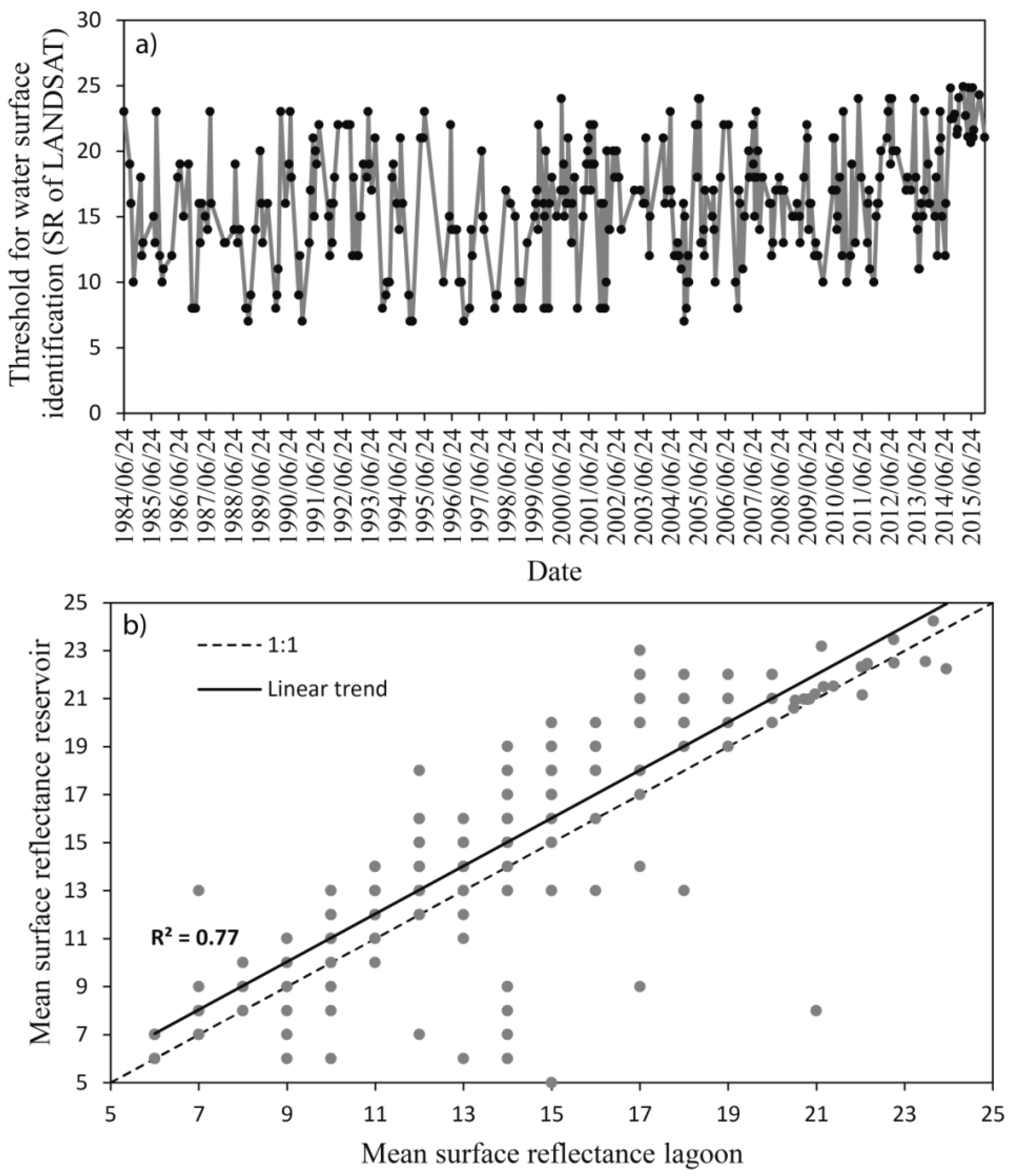
The threshold for water identification obtained for the LANDSAT images without errors and clouds is shown in Figure 5a. We also present the mean surface reflectance of the reservoir zone included in the calibration area vs. the mean surface reflectance area of the lagoon calibration area (see Figure 5b). They show similar values with good correlation (R2 of 0.77), but, in general, the reservoir has higher mean surface reflectance than the lagoon.
The surface water identified for the selected images in the studied period (1984–2015) (Figure 6a) was used to calculate the probability of being covered by water in each pixel (Figure 6b). We also verified that the pixels included in the calibration areas are always (for the studied period) covered by water. In general, the areas with lower elevation within the reservoir and the lagoons have a higher probability of being covered by water. The probability also increases in the areas located in the middle of the valley.
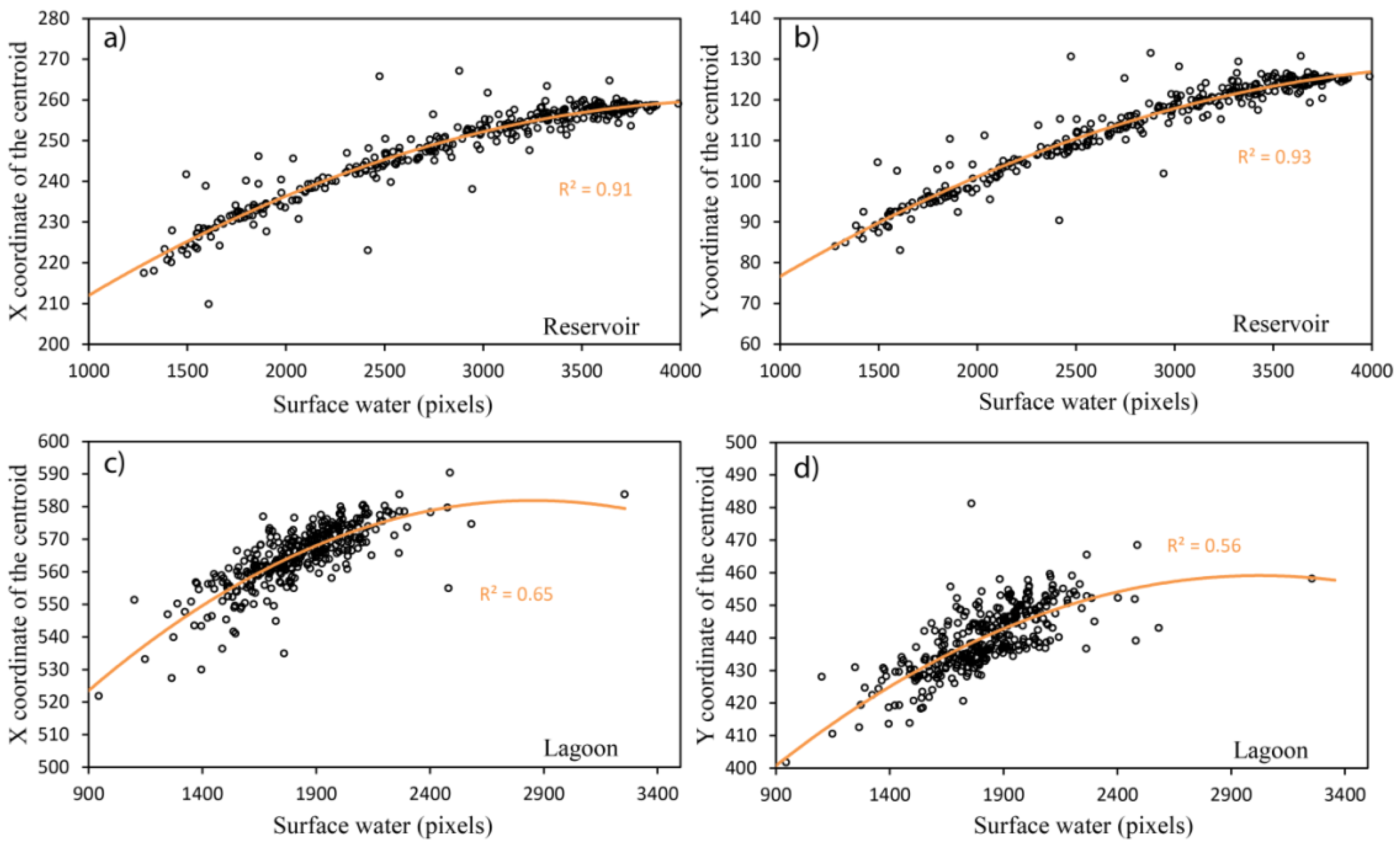
In order to know if a certain surface covered by water is related to the same distribution of pixels, we also studied the relationship between the surface water and the centroid of this area. In general, they show a good correlation. It is higher for the reservoir (see Figure 7a,b), which shows an R2 of higher than 0.91, than in the lagoons (Figure 7c,d), where the R2 is higher than 0.56.
We also wanted to complete the information within the period 2000–2015 by using information from the MODIS satellite. We used the same procedure (the entire methodology) that we used for LANDSAT but the results were not satisfactory. The correlation between the surface water identified by MODIS and LANDSAT is very poor (see Figure 8c). Note that the spatial resolution of MODIS (Figure 8b) is more than eight times that of the LANDSAT one (Figure 8a) (30 vs. 250 m), and the maximum width of our water bodies is around 350 m, in the reservoir, and 250 m in the lagoons. Taking into account these results, we used an alternative method to test the suitability of MODIS in the pilot that combines information from both sources of satellite data. For a certain image or day (i), we created a match with the other one (j) that produces the lower RMSE within the database, and we assigned the surface water of LANDSAT for day (j) to day (i). The correlation between the surface water identified by using LANDSAT individually and the surface water obtained by using this procedure is higher than the one obtained using only MODIS information (Figure 8d), but it is not good enough. Therefore, we decided not to use the MODIS information for water-cover area characterisation.

4.2. Surface Water from Regression Models

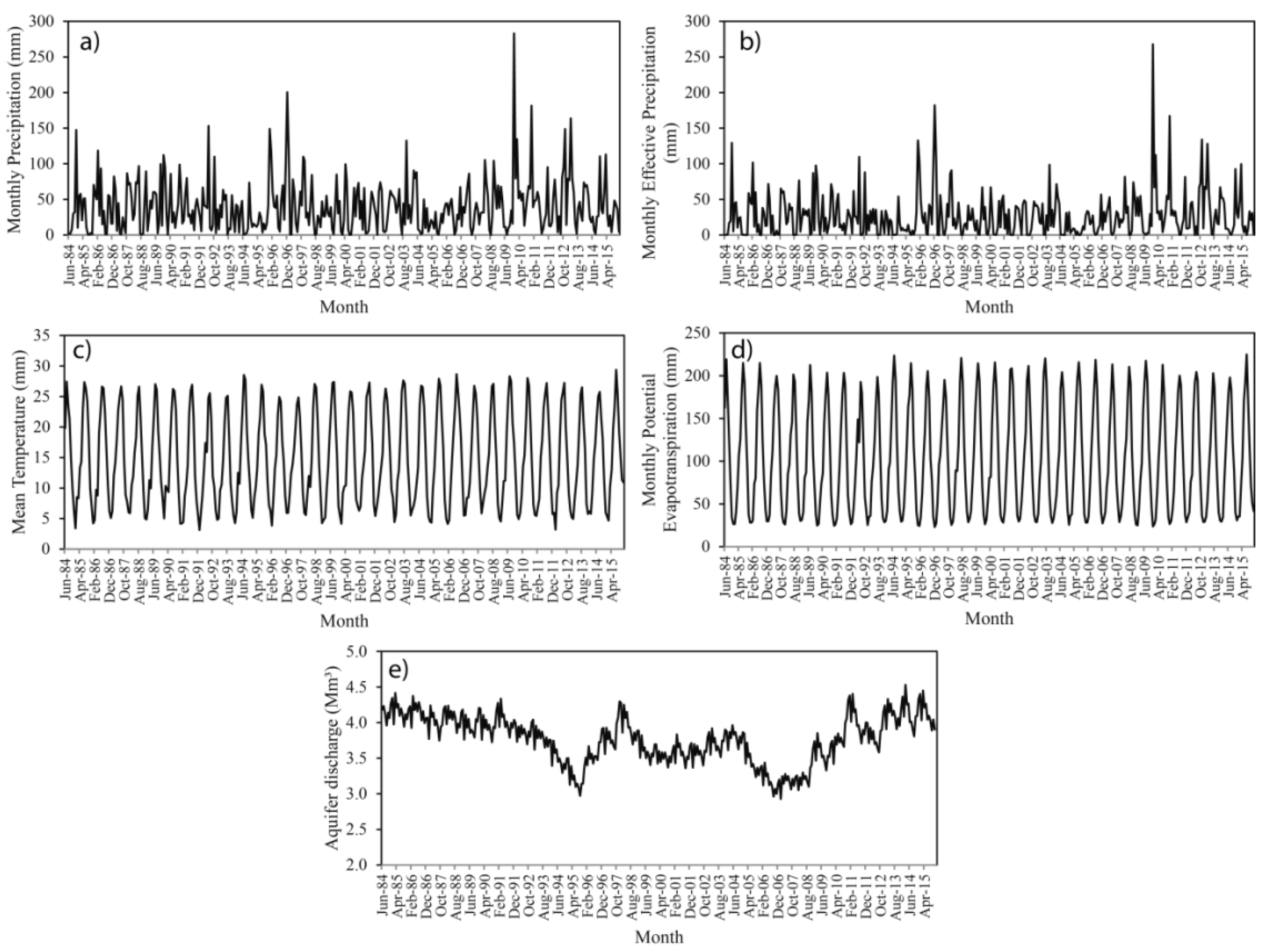
The 342 daily data obtained from LANDSAT were used to calculate the mean monthly surface water from June 1984 to December 2015. In this period, (384 months) there are 238 months with data and 146 gaps. The regression models selected to complete the gaps of information use five explanatory variables and the surface water of the previous month. The temporal series of these five explanatory variables are shown in Figure 9. The mean monthly precipitation in the period is 39.6 mm, whilst the effective precipitation (precipitation minus evapotranspiration) is 27.0 mm. The mean temperature and potential evapotranspiration are 14.9 °C and 102.6 mm, respectively. The mean monthly aquifer discharge to the wetland is 3.8 Mm3.
The six best regression models obtained for each regression structure considered are shown in Table 1. The final estimates were obtained by using an ensemble of these models. The R2 obtained in the calibration is similar for all of them, around 0.71. With respect to the different estimation modes, the performance statistics are also similar. In the forecasting mode the RMSE varies between 777.4 and 780.2 pixels. In the case of the forward completion the minimum and maximum RMSE are 497.4 and 501.8 pixels. It shows better results than the backward completion, which has an RMSE varying from 586.1 to 589.2 pixels. The best results for the completion mode are shown for the mixed version of forward–backward (RMSE from 475.6 to 477.6 pixels).
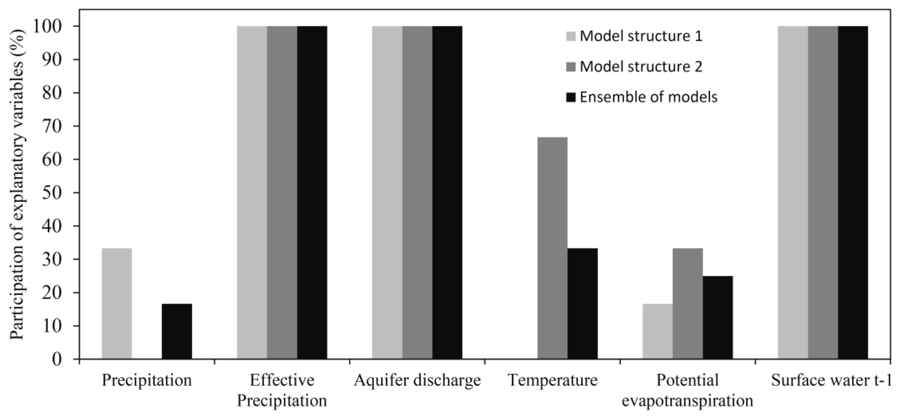
The participation of the explanatory variables in the ensemble of models is heterogeneous (Figure 10). Effective precipitation, aquifer discharge, and surface water of the previous month take part in all the regression models (100% participation). The participation of the rest of variables is lower. The precipitation is selected in 16.7% in the ensemble of models and temperature and potential evapotranspiration in 33.3% and 25.0%, respectively.
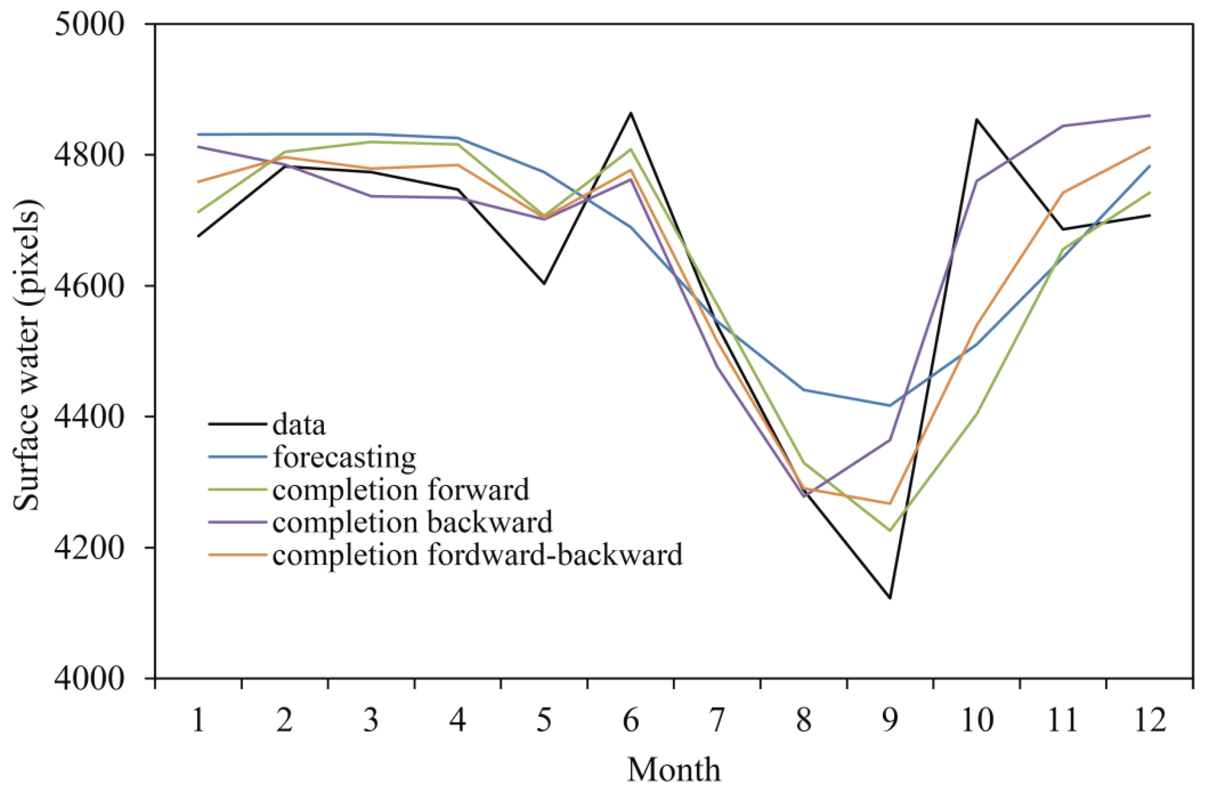
The calibration of the regression models was done by using 158 data of the 384 months in the study period. Note that we have 238 data, but our regression models can only be calibrated when the data of surface water are also available for the previous month. The experimental data and the estimation obtained by using the ensemble approach are shown in Figure 11a for the 158 months used in the calibration. Figure 11b also shows the 238 experimental data and the estimated values for the entire period (384 months) using the different estimation modes. As we commented previously the estimation mode that shows the best results is the forward–backward completion approach. This ensemble solution (see Section 2) shows a RMSE of 476 pixels. Figure 12 shows the experimental data and the estimation modes for the monthly mean year. An important reduction (13%) in surface water can be observed during the summertime (from July to September), which recovered during the autumn (from October to December). The rest of the year (from January to June), the mean surface water is more stable, with a value of around 4750 pixels, which is equivalent to 4.3 Km2.
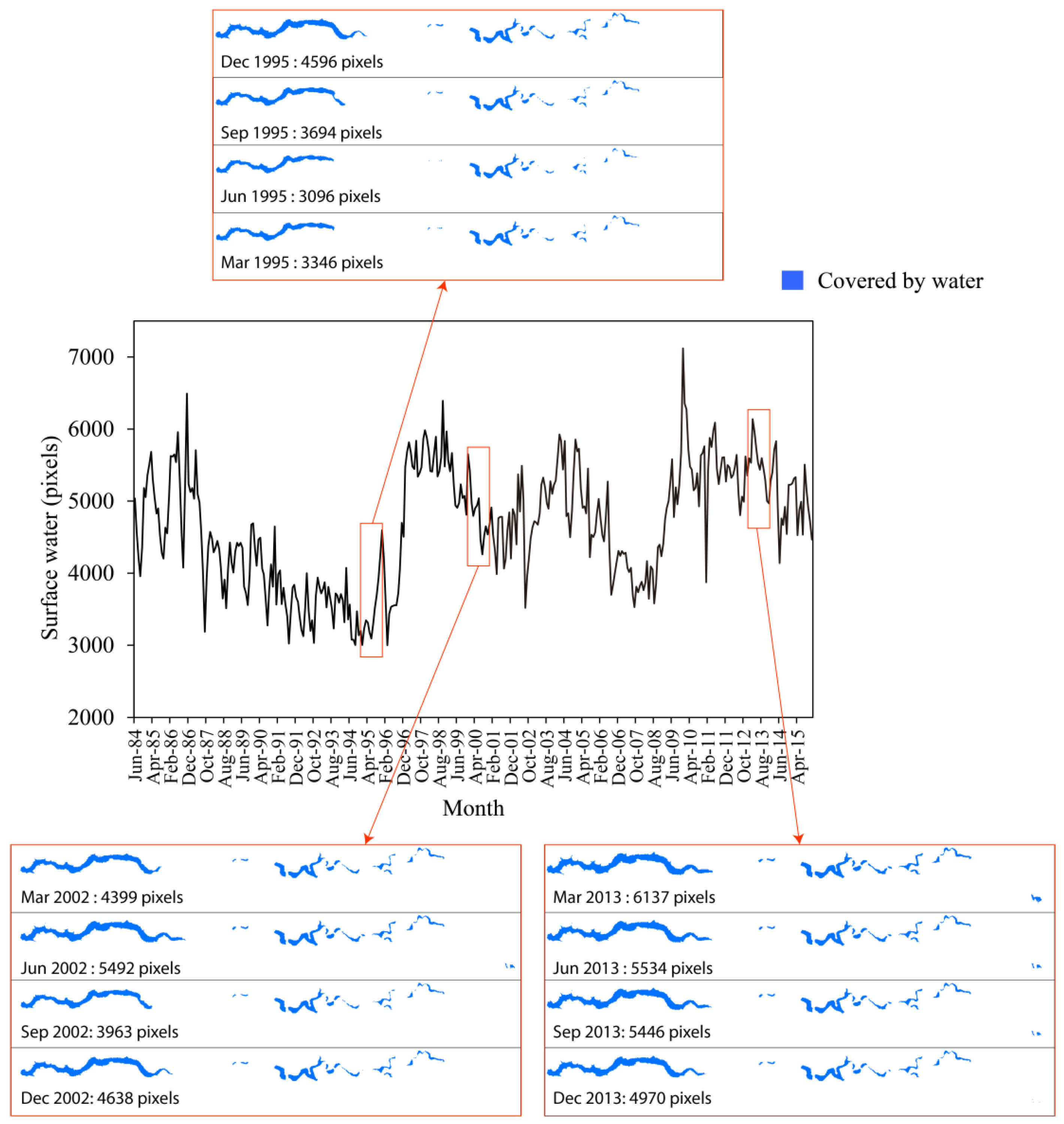
The final spatiotemporal estimation of the monthly surface water (the main objective of this study) was obtained by using the best solution, the forward–backward completion approach (see Figure 13). It shows the complete monthly time series of the estimated surface water and the spatial distribution for some months (March, June, September, and December) of a dry year (1995), a wet year (2013), and an average year (2002) of the studied period (1984–2015). For these years, the aquifer discharge and the mean surface water are 38.4 Mm3 and 3536 pixels, 49.4 Mm3 and 5518 pixels, and 43.1 Mm3 and 4635 pixels, respectively.

5. Discussion

We demonstrated the utility of the proposed methodology for mapping surface water in wetlands. It is a general method that could be applied in case studies where a good relationship between hydro-climatological variables and surface water is observed. In our case study we obtained an RMSE of around 476 pixels for the completion mode, which is equivalent to a 7% of the total lagoon surface. We consider that it is good enough and assume that the errors are acceptable taking into account the benefit of obtaining a complete monthly series of surface water.
We also showed that the spatial resolution required to use satellite data should be analysed for each case study, depending on the size of the water bodies. In our case study, the MODIS satellite data, which has a spatial resolution of 250 m, were not suitable. Note that the average width of the water bodies is around 250 m. However, the MODIS product has been used satisfactorily in cases studies with wider water bodies [46,47]. The LANDSAT data were useful in our case study, where the average width of the water bodies is around eight times the LANDSAT spatial resolution, whilst this rate is one for the MODIS data.
Other satellites launched recently (e.g., SENTINEL with 10 m resolution [48] or PLEIADES with 0.5 m resolution [49]) provide very detailed spatial information. However, they do not cover a long time period, which is needed for modelling purposes in some applications. This is another critical aspect for the selection of a satellite source of information. LANDSAT 5 (and the next missions) has a relatively good spatial resolution compared to the new satellites and was launched in 1984. It has been used in several earth surface applications (e.g., water detection [24], snow cover area [25] and land use change [26]).
However, the clouds and sensor errors did not allow us to obtain a continuous monthly series of surface water in our pilots in the study period (1984–2015) if we only used this source of information. A regression approach based on the values adopted by some hydro-climatological explanatory variables was used to overcome this drawback. It was defined with a mathematical structure analogous to the one used by Collados-Lara et al. [3,30] for the estimation of snow variables. This study has proved that the methodology is also suitable for completing data regarding surface water in wetlands.
The application of the proposed methodology to other case studies also requires the estimation of the surface reflectance threshold for water identification in an adequate calibration area for the water bodies included within the domain. In our case study, two different water bodies (reservoir and lagoons) were included. They showed some differences with respect the mean surface reflectance of the areas covered by water. This is due to the different depths of water in each body [50]. In our case study the depth of the reservoir was higher than the lagoons. Both areas also showed different behaviour when we studied the relationship between the spatial distribution of the surface water and its total value. Both water bodies show a good correlation between both variables, but in the case of the reservoir it was stronger. The reservoir always has the same pattern of filling and discharge (it works like a tank), but the lagoons have a more complex behaviour.

Limitations and Future Research

Although we have demonstrated the utility of the proposed approach for mapping surface water in wetlands, we want to highlight some limitations and future research.
(a)
This study was focused on estimating the monthly dynamic, but in some applications daily information can be necessary. The proposed regression approach cannot be used for daily completion. It uses the surface water of the previous time step and there are no consecutive days with data for the case study. For daily dynamic characterisation other approaches should be explored.
(b)
The proposed approach to complete surface water by using hydro-climatological variables requires a good correlation between these variables and the surface water. However, in other cases studies this correlation may not exist or the information of secondary variables may not be available (especially for the aquifer discharge which requires the calibration of a groundwater model).
(c)
The studied area highlights a strong conflict between groundwater-dependent ecosystems such as wetlands, and groundwater pumping to supply demands (mainly irrigation). This problem might be exacerbated in the future due to the impact of climate change. In this area a reduction in precipitation from 1.0 to 2.7% and an increase in temperature from 14.1 to 14.5% are expected for the period 2016–2045 with respect the period 1974–2015 considering the RCP8.5 emission scenario [15]. These changes will also have an impact on the surface water of the wetland. The proposed methodology is useful to propagate the impact on the explanatory hydro-climatological variables to the surface water through the proposed regression ensemble. This approach could be explored in future research.

6. Conclusions

We demonstrated the utility of a novel integrated method to approach monthly dynamic of surface water in wetlands. The approach can be applied to any case study where the following information is available: satellite data with adequate spatial resolution to identify the surface water distribution in different dates during a long enough period, and secondary variables that help to model the monthly system dynamic. The requirements that those data (spatial resolution of the satellite images and secondary variables) should fulfil will depend on the case study.
In our case study, Lagunas de Ruidera, the water bodies included in the wetland are narrow (maximum around 250 m) making the MODIS satellite (250 m resolution) unsuitable. Nevertheless, the LANDSAT satellite spatial resolution (30 m) and its temporal coverage (1984–2015) are also adequate for our proposed analyses. However, the monthly series obtained from LANDSAT has 38% of gaps due to its scarce revisit frequency (around 16 days), the errors, and clouds.
In this study we used a regression-based approach based on hydro-climatological explanatory variables to complete the surface water monthly series. The completion forward–backward mode showed the best results with a RMSE of 476 pixels (0.4 Km2). The explanatory variables that have a higher participation in the ensemble are effective precipitation, aquifer discharge and the surface water from the previous month. Other variables such as temperature, precipitation and potential evapotranspiration are included but with lower participation.
The proposed approach allowed us to simulate the surface water monthly dynamic for the Lagunas de Ruidera Ramsar wetland. The monthly mean year shows more or less stable mean surface water values around 4.3 Km2 during the period that goes from January to June. In summer months (from July to September) a mean reduction of around 13% can be observed, which then recovered during autumn (from October to December).
The proposed method can be extended in the future to propagate impacts of climate change on surface water distribution taking into account future climatic and hydrological scenarios in the definition of the explanatory variables. This extension could be explored in a future research. On the other hand, this study was focused on estimating the monthly dynamic, but in some applications daily information can be necessary. This issue is also open for future works.

Author Contributions

Conceptualisation, A.-J.C.-L., E.P.-I., and D.P.-V.; methodology, A.-J.C.-L., E.P.-I., D.P.-V., and L.B.-R.; software, A.-J.C.-L. and L.B.-R.; validation, A.-J.C.-L., L.B.-R., E.P.-I., and D.P.-V.; formal analysis, A.-J.C.-L., L.B.-R., E.P.-I., and D.P.-V.; investigation, A.-J.C.-L., L.B.-R., E.P.-I., and D.P.-V.; resources, A.-J.C.-L., L.B.-R., E.P.-I., and D.P.-V.; data curation, A.-J.C.-L., L.B.-R., E.P.-I., and D.P.-V.; writing—original draft preparation, A.-J.C.-L., L.B.-R., E.P.-I., and D.P.-V.; writing—review and editing, A.-J.C.-L., L.B.-R., E.P.-I., and D.P.-V.; visualisation, A.-J.C.-L.; supervision, E.P.-I., and D.P.-V.; project administration, D.P.-V.; funding acquisition, D.P.-V. All authors have read and agreed to the published version of the manuscript.

Funding

This research was partially supported by the research projects GeoE.171.008-TACTIC from GeoERA organisation funded by European Union’s Horizon 2020 research and innovation program and SIGLO-AN (RTI2018-101397-B-I00) from the Spanish Ministry of Science, Innovation and Universities (Programa Estatal de I+D+I orientada a los Retos de la Sociedad).

Data Availability Statement

The LANDSAT surface reflectance data (missions 5, 7, and 8) were retrieved from the United States Geological Survey www.usgs.gov (accessed on 27 April 2021) and the MODIS surface reflectance data (product MOD09GQ) were retrieved from the NASA Distributed Active Archive Center (DAAC) <earthdata.nasa.gov> (accessed on 27 April 2021). The precipitation and temperature data were obtained from the Spain02 (v5) project.

Conflicts of Interest

The authors declare no conflict of interest. The funders had no role in the design of the study; in the collection, analyses, or interpretation of data; in the writing of the manuscript, or in the decision to publish the results.

References

  1. Zhou, Y.; Dong, J.; Xiao, X.; Xiao, T.; Yang, Z.; Zhao, G.; Zou, Z.; Qin, Y. Open Surface Water Mapping Algorithms: A Comparison of Water-Related Spectral Indices and Sensors. Water 2017, 9, 256. [Google Scholar] [CrossRef]
  2. Colditz, R.R.; Souza, C.T.; Vazquez, B.; Wickel, A.J.; Ressl, R. Analysis of optimal thresholds for identification of open water using MODIS-derived spectral indices for two coastal wetland systems in Mexico. Int. J. Appl. Earth Obs. Geoinf. 2018, 70, 13–24. [Google Scholar] [CrossRef]
  3. Collados-Lara, A.-J.; Pardo-Igúzquiza, E.; Pulido-Velazquez, D. Spatiotemporal estimation of snow depth using point data from snow stakes, digital terrain models, and satellite data. Hydrol. Process. 2017, 31, 1966–1982. [Google Scholar] [CrossRef]
  4. Pardo-Igúzquiza, E.; Collados-Lara, A.-J.; Pulido-Velazquez, D. Estimation of the spatiotemporal dynamics of snow covered area by using cellular automata models. J. Hydrol. 2017, 550, 230–238. [Google Scholar] [CrossRef]
  5. Pflugmacher, D.; Rabe, A.; Peters, M.; Hostert, P. Mapping pan-European land cover using Landsat spectral-temporal metrics and the European LUCAS survey. Remote Sens. Environ. 2019, 221, 583–595. [Google Scholar] [CrossRef]
  6. He, B.-J.; Zhao, Z.-Q.; Shen, L.-D.; Wang, H.-B.; Li, L.-G. An approach to examining performances of cool/hot sources in mitigating/enhancing land surface temperature under different temperature backgrounds based on landsat 8 image. Sustain. Cities Soc. 2019, 44, 416–427. [Google Scholar] [CrossRef]
  7. Matthews, G.V.T. The Ramsar Convention on Wetlands: Its History and Development; Ramsar Convention Bureau: Gland, Switzerland, 1993; ISBN 2940073007. [Google Scholar]
  8. He, B.-J.; Zhu, J.; Zhao, D.-X.; Gou, Z.-H.; Qi, J.-D.; Wang, J. Co-benefits approach: Opportunities for implementing sponge city and urban heat island mitigation. Land Use Policy 2019, 86, 147–157. [Google Scholar] [CrossRef]
  9. De La Hera, A.; Gimena, E.C.; Cortés, À.G. Evaluating ecosystem services and drivers of change in Spanish groundwater-related wetlands included in the Ramsar Convention. AIMS Environ. Sci. 2017, 4, 232–250. [Google Scholar] [CrossRef]
  10. Anand, V.; Oinam, B. Future land use land cover prediction with special emphasis on urbanization and wetlands. Remote Sens. Lett. 2020, 11, 225–234. [Google Scholar] [CrossRef]
  11. Malekmohammadi, B.; Jahanishakib, F. Vulnerability assessment of wetland landscape ecosystem services using driver-pressure-state-impact-response (DPSIR) model. Ecol. Indic. 2017, 82, 293–303. [Google Scholar] [CrossRef]
  12. Baena-Ruiz, L.; Pulido-Velazquez, D.; Collados-Lara, A.-J.; Renau-Pruñonosa, A.; Morell, I. Global Assessment of Seawater Intrusion Problems (Status and Vulnerability). Water Resour. Manag. 2018, 32, 2681–2700. [Google Scholar] [CrossRef]
  13. Renau-Pruñonosa, A.; Morell, I.; Pulido-Velazquez, D. A Methodology to Analyse and Assess Pumping Management Strategies in Coastal Aquifers to Avoid Degradation Due to Seawater Intrusion Problems. Water Resour. Manag. 2016, 30, 4823–4837. [Google Scholar] [CrossRef] [Green Version]
  14. Collados-Lara, A.-J.; Pulido-Velazquez, D.; Pardo-Igúzquiza, E. An Integrated Statistical Method to Generate Potential Future Climate Scenarios to Analyse Droughts. Water 2018, 10, 1224. [Google Scholar] [CrossRef] [Green Version]
  15. Pulido-Velazquez, D.; Collados-Lara, A.-J.; Alcalá, F.J. Assessing impacts of future potential climate change scenarios on aquifer recharge in continental Spain. J. Hydrol. 2018, 567, 803–819. [Google Scholar] [CrossRef]
  16. Pulido-Velazquez, D.; Renau-Pruñonosa, A.; Llopis-Albert, C.; Morell, I.; Collados-Lara, A.-J.; Senent-Aparicio, J.; Baena-Ruiz, L. Integrated assessment of future potential global change scenarios and their hydrological impacts in coastal aquifers—A new tool to analyse management alternatives in the Plana Oropesa-Torreblanca aquifer. Hydrol. Earth Syst. Sci. 2018, 22, 3053–3074. [Google Scholar] [CrossRef] [Green Version]
  17. Escriva-Bou, A.; Pulido-Velazquez, M.; Pulido-Velazquez, D. Economic Value of Climate Change Adaptation Strategies for Water Management in Spain’s Jucar Basin. J. Water Resour. Plan. Manag. 2017, 143, 04017005. [Google Scholar] [CrossRef]
  18. Baena-Ruiz, L.; Pulido-Velazquez, D.; Collados-Lara, A.-J.; Renau-Pruñonosa, A.; Morell, I.; Senent-Aparicio, J.; Llopis-Albert, C. Summarizing the impacts of future potential global change scenarios on seawater intrusion at the aquifer scale. Environ. Earth Sci. 2020, 79, 1–13. [Google Scholar] [CrossRef]
  19. Vuolo, F.; Żółtak, M.; Pipitone, C.; Zappa, L.; Wenng, H.; Immitzer, M.; Weiss, M.; Baret, F.; Atzberger, C. Data Service Platform for Sentinel-2 Surface Reflectance and Value-Added Products: System Use and Examples. Remote Sens. 2016, 8, 938. [Google Scholar] [CrossRef] [Green Version]
  20. Vermote, E.; Justice, C.; Claverie, M.; Franch, B. Preliminary analysis of the performance of the Landsat 8/OLI land surface reflectance product. Remote Sens. Environ. 2016, 185, 46–56. [Google Scholar] [CrossRef] [PubMed]
  21. Zhan, X.; Sohlberg, R.; Townshend, J.; DiMiceli, C.; Carroll, M.; Eastman, J.; Hansen, M.; DeFries, R. Detection of land cover changes using MODIS 250 m data. Remote Sens. Environ. 2002, 83, 336–350. [Google Scholar] [CrossRef]
  22. Xiao, F.; Cheng, W.; Zhu, L.; Feng, Q.; Du, Y. Downscaling MODIS-derived water maps with high-precision topographic data in a shallow lake. Int. J. Remote Sens. 2018, 39, 7846–7860. [Google Scholar] [CrossRef]
  23. Che, X.; Yang, Y.; Feng, M.; Xiao, T.; Huang, S.; Xiang, Y.; Chen, Z. Mapping Extent Dynamics of Small Lakes Using Downscaling MODIS Surface Reflectance. Remote Sens. 2017, 9, 82. [Google Scholar] [CrossRef] [Green Version]
  24. Rokni, K.; Ahmad, A.; Selamat, A.; Hazini, S. Water Feature Extraction and Change Detection Using Multitemporal Landsat Imagery. Remote Sens. 2014, 6, 4173–4189. [Google Scholar] [CrossRef] [Green Version]
  25. Girona-Mata, M.; Miles, E.S.; Ragettli, S.; Pellicciotti, F. High-Resolution Snowline Delineation From Landsat Imagery to Infer Snow Cover Controls in a Himalayan Catchment. Water Resour. Res. 2019, 55, 6754–6772. [Google Scholar] [CrossRef] [Green Version]
  26. Alam, A.; Bhat, M.S.; Maheen, M. Using Landsat satellite data for assessing the land use and land cover change in Kashmir valley. GeoJournal 2020, 85, 1529–1543. [Google Scholar] [CrossRef] [Green Version]
  27. Jolly, I.D.; McEwan, K.L.; Holland, K.L. A review of groundwater-surface water interactions in arid/semi-arid wetlands and the consequences of salinity for wetland ecology. Ecohydrology 2008, 1, 43–58. [Google Scholar] [CrossRef]
  28. Collados-Lara, A.-J.; Pardo-Igúzquiza, E.; Pulido-Velazquez, D.; Jiménez-Sánchez, J. Precipitation fields in an alpine Mediterranean catchment: Inversion of precipitation gradient with elevation or undercatch of snowfall? Int. J. Clim. 2018, 38, 3565–3578. [Google Scholar] [CrossRef]
  29. Jimeno-Sáez, P.; Pulido-Velazquez, D.; Collados-Lara, A.-J.; Pardo-Igúzquiza, E.; Senent-Aparicio, J.; Baena-Ruiz, L. A Preliminary Assessment of the “Undercatching” and the Precipitation Pattern in an Alpine Basin. Water 2020, 12, 1061. [Google Scholar] [CrossRef] [Green Version]
  30. Collados-Lara, A.-J.; Pulido-Velazquez, D.; Pardo-Igúzquiza, E.; Alonso-González, E. Estimation of the spatiotemporal dynamic of snow water equivalent at mountain range scale under data scarcity. Sci. Total Environ. 2020, 741, 140485. [Google Scholar] [CrossRef] [PubMed]
  31. Pérez-Sánchez, J.; Senent-Aparicio, J.; Segura-Méndez, F.; Pulido-Velazquez, D.; Srinivasan, R. Evaluating Hydrological Models for Deriving Water Resources in Peninsular Spain. Sustainability 2019, 11, 2872. [Google Scholar] [CrossRef] [Green Version]
  32. Pulido-Velazquez, D.; Sahuquillo, A.; Andreu, J.; Pulido-Velazquez, M. A general methodology to simulate groundwater flow of unconfined aquifers with a reduced computational cost. J. Hydrol. 2007, 338, 42–56. [Google Scholar] [CrossRef]
  33. Senent-Aparicio, J.; López-Ballesteros, A.; Pérez-Sánchez, J.; Segura-Méndez, F.J.; Pulido-Velazquez, D. Using Multiple Monthly Water Balance Models to Evaluate Gridded Precipitation Products over Peninsular Spain. Remote Sens. 2018, 10, 922. [Google Scholar] [CrossRef] [Green Version]
  34. Senent-Aparicio, J.; Sáez, P.J.; Bueno-Crespo, A.; Pérez-Sánchez, J.; Pulido-Velázquez, D. Coupling machine-learning techniques with SWAT model for instantaneous peak flow prediction. Biosyst. Eng. 2019, 177, 67–77. [Google Scholar] [CrossRef]
  35. Pulido-Velazquez, D.; Garrote, L.; Andreu, J.; Martin-Carrasco, F.-J.; Iglesias, A. A methodology to diagnose the effect of climate change and to identify adaptive strategies to reduce its impacts in conjunctive-use systems at basin scale. J. Hydrol. 2011, 405, 110–122. [Google Scholar] [CrossRef]
  36. Santos, F.; Peña, A.; Nogales, B.; Soria-Soria, E.; del Cura, M.; Ángeles, G.; González-Martín, J.A.; Antón, J. Bacterial diversity in dry modern freshwater stromatolites from Ruidera Pools Natural Park, Spain. Syst. Appl. Microbiol. 2010, 33, 209–221. [Google Scholar] [CrossRef] [PubMed]
  37. Foster, J.S.; Green, S.J. Microbial Diversity in Modern Stromatolites; Springer Science and Business Media LLC: Berlin, Germany, 2011; pp. 383–405. [Google Scholar]
  38. Pulido-Velazquez, D.; Sahuquillo, A.; Andreu, J. A two-step explicit solution of the Boussinesq equation for efficient simulation of unconfined aquifers in conjunctive-use models. Water Resour. Res. 2006, 42. [Google Scholar] [CrossRef]
  39. Pulido-Velazquez, D.; Sahuquillo, A.; Andreu, J.; Pulido-Velazquez, M. An efficient conceptual model to simulate surface water body-aquifer interaction in conjunctive use management models. Water Resour. Res. 2007, 43. [Google Scholar] [CrossRef]
  40. Llopis-Albert, C.; Pulido-Velazquez, D. Using MODFLOW code to approach transient hydraulic head with a sharp-interface solution. Hydrol. Process. 2015, 29, 2052–2064. [Google Scholar] [CrossRef]
  41. McCormack, T.; Naughton, O.; Johnston, P.M.; Gill, L. Quantifying the influence of surface water–groundwater interaction on nutrient flux in a lowland karst catchment. Hydrol. Earth Syst. Sci. 2016, 20, 2119–2133. [Google Scholar] [CrossRef] [Green Version]
  42. Hardy, A.; Oakes, G.; Ettritch, G. Tropical Wetland (TropWet) Mapping Tool: The Automatic Detection of Open and Vegetated Waterbodies in Google Earth Engine for Tropical Wetlands. Remote Sens. 2020, 12, 1182. [Google Scholar] [CrossRef] [Green Version]
  43. Herrera, S.; Gutiérrez, J.M.; Ancell, R.; Pons, M.R.; Frías, M.D.; Fernández, J. Development and analysis of a 50-year high-resolution daily gridded precipitation dataset over Spain (Spain02). Int. J. Clim. 2010, 32, 74–85. [Google Scholar] [CrossRef] [Green Version]
  44. Herrera, S.; Fernández, J.; Gutiérrez, J.M. Update of the Spain02 gridded observational dataset for EURO-CORDEX evaluation: Assessing the effect of the interpolation methodology. Int. J. Clim. 2016, 36, 900–908. [Google Scholar] [CrossRef] [Green Version]
  45. Hargreaves, G.H.; Allen, R.G. History and Evaluation of Hargreaves Evapotranspiration Equation. J. Irrig. Drain. Eng. 2003, 129, 53–63. [Google Scholar] [CrossRef]
  46. Khandelwal, A.; Karpatne, A.; Marlier, M.E.; Kim, J.; Lettenmaier, D.P.; Kumar, V. An approach for global monitoring of surface water extent variations in reservoirs using MODIS data. Remote Sens. Environ. 2017, 202, 113–128. [Google Scholar] [CrossRef]
  47. Di Vittorio, C.A.; Georgakakos, A.P. Land cover classification and wetland inundation mapping using MODIS. Remote Sens. Environ. 2018, 204, 1–17. [Google Scholar] [CrossRef]
  48. Huang, W.; DeVries, B.; Huang, C.; Lang, M.W.; Jones, J.W.; Creed, I.F.; Carroll, M.L. Automated Extraction of Surface Water Extent from Sentinel-1 Data. Remote Sens. 2018, 10, 797. [Google Scholar] [CrossRef] [Green Version]
  49. Luo, Y.; Doxaran, D.; Vanhellemont, Q. Retrieval and Validation of Water Turbidity at Metre-Scale Using Pléiades Satellite Data: A Case Study in the Gironde Estuary. Remote Sens. 2020, 12, 946. [Google Scholar] [CrossRef] [Green Version]
  50. Stumpf, R.P.; Holderied, K.; Sinclair, M. Determination of water depth with high-resolution satellite imagery over variable bottom types. Limnol. Oceanogr. 2003, 48, 547–556. [Google Scholar] [CrossRef]
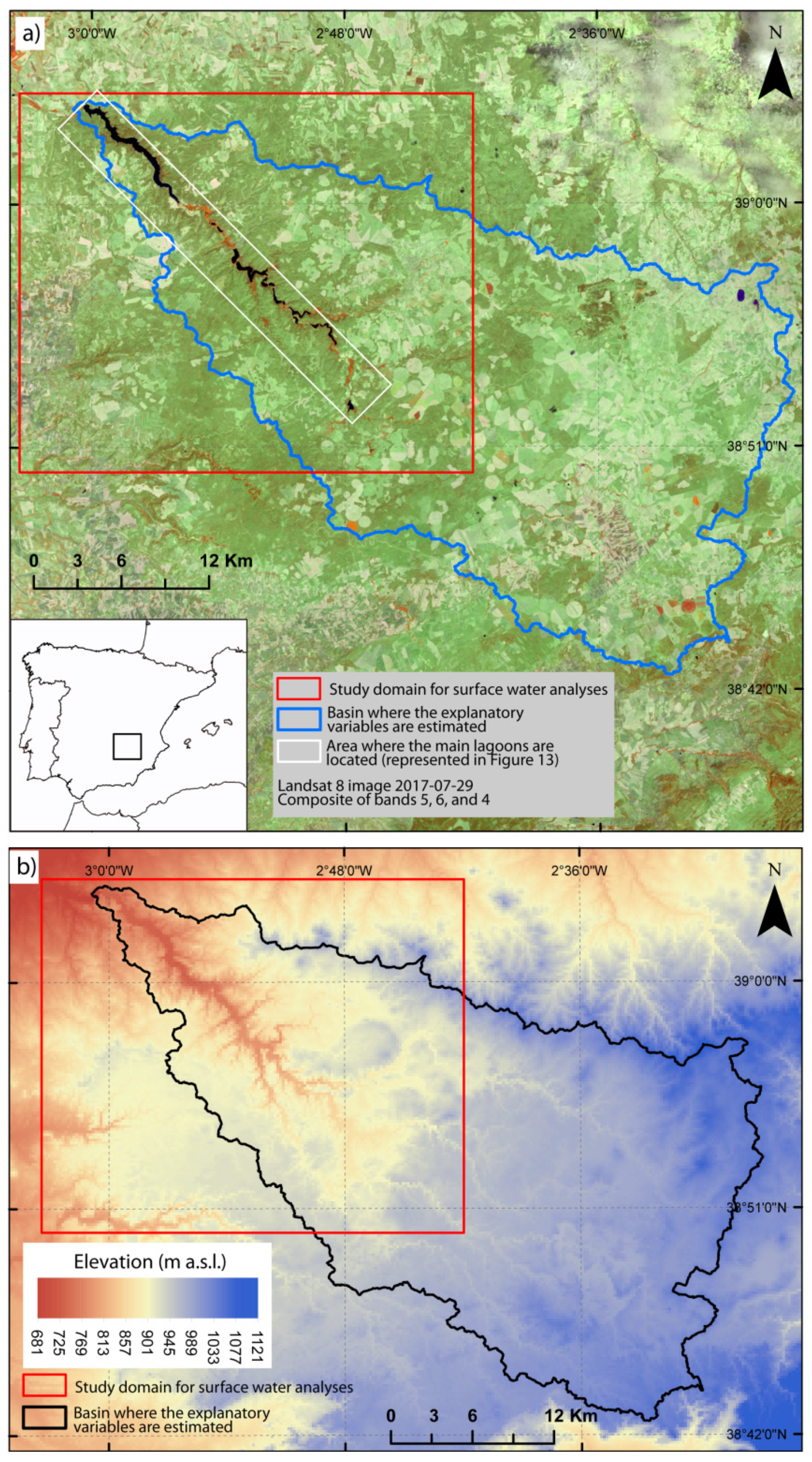
Figure 1. Study area: (a) location; (b) digital elevation model of the area.
Remotesensing 13 02380 g001
Figure 2. Flow chart of the proposed methodology.
Remotesensing 13 02380 g002
Figure 3. Surface reflectance maps for the case study and the areas used for calibration: (a) image without errors and clouds; (b) discarded image due to errors; (c) discarded image due to a wrong geo-referenced; (d) discarded image due to errors and clouds.
Remotesensing 13 02380 g003
Figure 4. Spatial distribution of the surface water within the period 1984 to 2015: (a) maximum surface water; (b) minimum surface water.
Remotesensing 13 02380 g004
Figure 5. Surface reflectance of the calibration areas: (a) temporal dynamic of the surface reflectance threshold used to identify the surface water; (b) comparison of the mean surface reflectance of the two areas used for calibration.
Remotesensing 13 02380 g005
Figure 6. Surface water in the period 1984 to 2015: (a) surface water identified by using LANDSAT for the days with available information; (b) spatial distribution of the probability of being covered by water (days with water divided by the total days in the studied period) within a pixel. (b1) Zoom in on (b) to show the reservoir area, (b2) Zoom in on (b) to show the lagoons area.
Remotesensing 13 02380 g006
Figure 7. Relationship between the number of pixels covered by water and the centroid of the surface water: (a) for the X coordinate within the reservoir; (b) for the Y coordinate within the reservoir; (c) for the X coordinate within the lagoon areas; (d) for the Y coordinate within the lagoon areas.
Remotesensing 13 02380 g007
Figure 8. Surface reflectance map for the day 2015-03-10: (a) from LANDSAT; (b) from MODIS. Monthly surface water identified by LANDSAT vs. MODIS: (c) using them independently; (d) using matches of images.
Remotesensing 13 02380 g008
Figure 9. Explanatory variables used for the calibration of the multiple regression model in the period 1984 to 2015: (a) precipitation; (b) effective precipitation; (c) temperature; (d) potential evapotranspiration; (e) aquifer discharge.
Remotesensing 13 02380 g009
Figure 10. Participation of the explanatory variables in the regression models.
Remotesensing 13 02380 g010
Figure 11. Obtained root mean squared error (RMSE) for the ensemble of regression models: (a) calibration; (b) cross-validation.
Remotesensing 13 02380 g011
Figure 12. Mean year of the monthly dynamic of the surface water obtained by using the different estimation modes for the ensemble of regression models.
Remotesensing 13 02380 g012
Figure 13. Monthly time series of the estimated surface water for the study period (1985–2015) and spatial distribution of the surface water for some months (March, June, September, and December) of a dry year (1995), an average year (2002), and a wet year (2013). The area used for the spatial representation is shown as a white square in Figure 1.
Remotesensing 13 02380 g013
Table 1. Regression models used to obtain the ensemble and its performance in terms of R2 in the calibration and RMSE in the re-analysis. P is precipitation, PE is effective precipitation, T is temperature, E is potential evapotranspiration, D is aquifer discharge, and W is the surface water in the previous month.
ModelxixjxlxkR² CalibrationRMSE (Pixels) ForecastingRMSE (Pixels) Completion ForwardRMSE (Pixels) Completion BackwardRMSE (Pixels) Completion Forward–Backward
1.1(D)(W)(PE)LOG(D)0.709777.374497.764589.183476.856
1.2(W)LOG(D)1/(P)(PE)20.707777.878501.515586.689477.398
1.3(D)(W)(PE)SQRT(D)0.709778.372498.137588.780476.825
1.4(W)(PE)LOG(W)1/(D)0.709778.419498.782588.137476.714
1.5(D)(W)1/(P)(PE)20.707778.557501.822587.120477.638
1.6(W)1/(D)1/(PE)(PE)20.709778.733498.290587.081476.276
2.1(W)(PE)1/(D)1/(T)0.709778.41497.683586.064475.621
2.2(W)(PE)LOG(D)1/(T)0.709779.114497.983586.479475.854
2.3(W)(PE)1/(D)1/(E)0.709779.45497.351587.411476.175
2.4(W)(PE)1/(T)SQRT(D)0.709779.497498.125586.684475.965
2.5(D)(W)(PE)1/(T)0.709779.849498.280586.919476.094
2.6(W)(PE)LOG(D)1/(E)0.709780.244497.652587.810476.400
Publisher’s Note: MDPI stays neutral with regard to jurisdictional claims in published maps and institutional affiliations.