Revising the Observation Satellite Scheduling Problem Based on Deep Reinforcement Learning

Abstract

Earth observation satellite task scheduling research plays a key role in space-based remote sensing services. An effective task scheduling strategy can maximize the utilization of satellite resources and obtain larger objective observation profits. In this paper, inspired by the success of deep reinforcement learning in optimization domains, the deep deterministic policy gradient algorithm is adopted to solve a time-continuous satellite task scheduling problem. Moreover, an improved graph-based minimum clique partition algorithm is proposed for preprocessing in the task clustering phase by considering the maximum task priority and the minimum observation slewing angle under constraint conditions. Experimental simulation results demonstrate that the deep reinforcement learning-based task scheduling method is feasible and performs much better than traditional metaheuristic optimization algorithms, especially in large-scale problems.

1. Introduction

Earth observation satellites (EOSs) are platforms equipped with optical instruments in order to take photographs of specific areas at the request of users [1]. Currently, EOSs have been extensively employed in scientific research, mainly in environment and disaster surveillance [2], ocean monitoring [3], agricultural harvesting [4], etc. However, with the increase in multi-user and multi-satellite space application scenarios [5,6], it is becoming more difficult to meet various observation requirements under the limitation of satellite resources. Therefore, an effective EOS scheduling algorithm plays an important role to improve high-quality space-based information services, and not only guides the corresponding EOSs on how to perform the following actions, but also controls the time to start the observations [5]. The main purpose is to maximize the observation profit within the limited observation time window and with other resources (for example, the available energy, the remaining data storage, etc.) [7,8].

The EOS scheduling problem (EOSSP) is well known as a complex non-deterministic polynomial (NP) hard problem and multiple objective combinational optimization problem [9,10]. Currently, inspired by increasing demands on scheduling EOSs effectively and efficiently, the study of the EOSSP has gained more and more attention. Wang et al. [7] summarized that the EOSSP could be divided into time-continuous and time-discrete problems. In time-continuous models [11,12,13], a continuous decision variable is introduced to represent the observation start time for each visible time window (VTW), which is defined to check whether tasks are scheduled or not. On the other hand, for time-discrete models [14,15,16], each time window generates multiple observation tasks for the same target. In this way, each candidate task has a determined observation time, and binary decision variables are introduced to represent whether a task is operated in a specific time slice.

General solving algorithms are usually classified into exact method, heuristic, metaheuristic [17,18] and machine learning [7]. Exact methods, such as branch and bound (BB) [19] and mixed integer linear programming (MILP) [15], have deterministic solving steps and could solve problems in polynomial time, but it is nearly impossible to build a deterministic model for a larger scale problem. Heuristic methods can be used to speed up the process by finding a satisfactory solution, but this method depends on a specific heuristic policy and the policy is not always feasible. Jang et al. [20] proposed a heuristic solution approach to solve the image collection planning problem of the KOMPSAT-2 satellite. Liu et al. [21] combined the neural network method and heuristic search algorithm and the result was superior to the existing heuristic search algorithm in terms of the overall profit. Alternatively, without relying on a specific heuristic policy, metaheuristic methods could provide a sufficiently high-quality and universal solution to an optimization problem. For example, Kim et al. [22] proposed an optimal algorithm based on a genetic algorithm for synthetic aperture radar (SAR) imaging satellite constellation scheduling. Niu et al. [23] presented a multi-objective genetic algorithm to solve the problem of satellite areal task scheduling during disaster emergency responses. Long et al. [24] proposed a two-phase GA–SA hybrid algorithm for the EOSSP which is superior to the GA or SA algorithm alone. Although metaheuristic algorithms could gain better operation results and have been widely adopted in the EOSSP, they easily fall into local optimum [25] due to the dependence on one certain mathematical model. Consequently, this makes us turn to deep reinforcement learning (DRL), which is known as a model-free solution and can autonomously build a general task scheduling strategy by training [26]. It has the promising potential to be applied in combinatorial optimization problems [27,28,29].

As a significant research domain in machine learning, DRL has achieved success in game playing and robot control. Moreover, recently, DRL has also gained more and more attention in optimization domains. Bello et al. [27] presented a DRL framework using neural networks and a policy gradient algorithm for solving problems modeled as the traveling salesman problem (TSP). Additionally, for the TSP, Khalil et al. [28] embedded a graph in DRL networks and it learnt effective policies. Furthermore, Nazari et al. [29] gave an end-to-end framework with a parameterized stochastic policy for solving the vehicle routing problem (VRP), which is an expanded problem based on the TSP. Peng et al. [30] presented a dynamic attention model with dynamic encoder–decoder architecture and obtained a good generalization performance in the VRP. Besides the TSP and VRP, another type of optimization problem, resource allocation [25], also has been solved by RL. Khadilkar et al. [31] adopted RL to schedule time resourced for a railway system, and it was found that the Q-learning algorithm is superior to heuristic approaches in effectiveness. Ye et al. [32] proposed a decentralized resource allocation mechanism for vehicle-to-vehicle communications based on DRL and improved the communication resource allocation.

Inspired by the above applications of DRL, solving the EOSSP by using DRL has become a feasible solution. Hadj-Salah et al. [33] adopted A2C to handle the EOSSP in order to reduce the time to completion of large-area requests. Wang et al. [34] proposed a real-time online scheduling method for image satellites by importing A3C into satellite scheduling. Zhao et al. [35] developed a two-phase neural combinatorial optimization RL method to address the EOSSP with the consideration of the transition time constraint and image quality criteria. Lam et al. [36] proposed a training system based on RL which is fast enough to generate decisions in near real time.

In the present paper, the EOS scheduling problems as a time-continuous model with multiple constraints are revised by adopting the deep deterministic policy gradient (DDPG) algorithm, and comparisons with the traditional metaheuristic methods are conducted with an increase in the task scale. The major highlights are summarized as follows:

• Aiming to enhance the task scheduling efficiency further, an improved graph-based minimum clique partition algorithm is introduced as a task clustering preprocess to decrease the task scale and improve the scheduling algorithm’s effect.
• Different from previous studies, the EOSSP was considered as a time-discrete model when solving by RL algorithms. In this paper, a time-continuous model is established for the EOSSP, which could make accurate observation time decisions for each task by the DDPG algorithm.
• Considering practical engineering constraints, comparison experiments were implemented between the RL method and some metaheuristic methods, such as the GA, SA and GA–SA hybrid algorithm, to validate the feasibility of the DDPG algorithm.

2. Problem Description

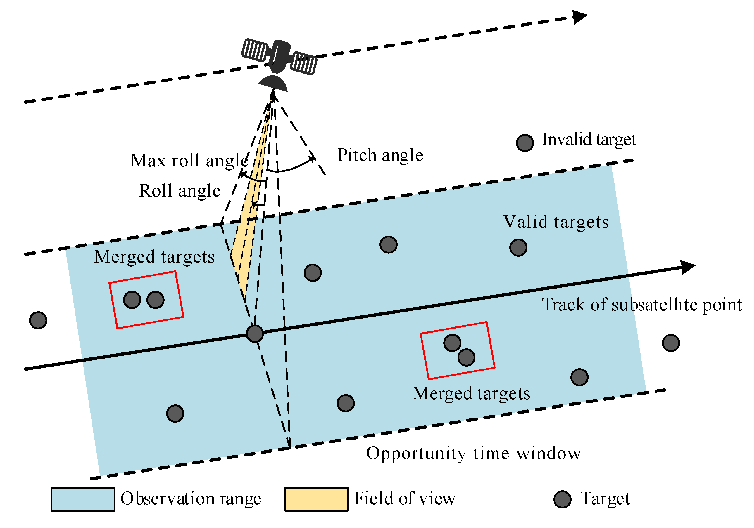
As shown in Figure 1, an EOS can maneuver in the direction of three axes (roll, pitch and yaw) for transitions between every two sequential observation tasks. Usually, the mobility of the roll angle represents the slewing maneuverability of the EOS. The maneuvering of the pitch angle enables the targets to be observed in advance or over time. Observation targets are accessible within a period of a specific VTW, which is determined by the maximum off-nadir angle. The observation window (OW) defines the start and the end time for observing target in the VTW. Therefore, the task scheduling algorithm enables an EOS to conduct certain operations for the transformation between two sequential observation tasks, such as slew maneuvering and payload switching. Simultaneously, observation tasks are restricted in a specific time interval, and the observations must be carried out continuously and completely within the VTW [37].

It is noted that targets outside the observation range are invisible, and are be seen as invalid, as shown in Figure 1. An EOS could observe multiple targets simultaneously, and the observation task of the merged targets is defined as a clustered task in this study. Task clustering belongs to preprocessing for EOS task scheduling, which has gained more and more attention as it enables an EOS to finish more tasks at the cost of relatively few optical sensor opening times and satellite maneuver times. To clearly explain the EOSSP, herein, a summary of the most important notations in this paper is given in

Table 1. Summary of notations.

Symbol	Meaning
$t_u$	Observation task to target u
$t_u^c$	Observation task to merged target u
$[TW{S}_u^i,TW{E}_u^i]$	VTW of $t_u$ in the $i$th orbit
$[TW{S}_u^{ci},TW{E}_u^{ci}]$	VTW of $t_u^c$ in the $i$th orbit
${\theta }_u$	Slewing angle for observation task $t_u$
$d_u$	Observation duration time of $t_u$
$x_u$	Whether to execute $t_u$
$x_{uv}$	Whether to transform execution from $t_u$ to $t_v$
$v_s$	Slewing maneuver velocity
$s_{uv}$	Preparation time of task switch
$tran{T}_{uv}$	Slewing angle maneuver time between two tasks
$maxT$	Maximum operating time in one observation
$max\theta$	Maximum slewing angle
$c_i$	Storage consumption per unit observation time
M	Total data storage capacity
$e_i$	Energy consumption per unit time of observation
${\epsilon }_{uv}$	Energy consumption per unit time of slewing maneuver
E	Total available energy
$pri{o}_u$	Priority of observation task $t_u$

.

2.1. Graph Clustering Model

In contrast to task scheduling without clustering, this strategy could save a lot of energy, especially with frequent observations. In addition, task clustering enables some previously conflicting tasks to be executed at the same time. The condition for merging multiple tasks into a clustering task is that these tasks can be finished with the same slewing angle and OW [38], which constrains the task clustering process.

(1) Time window-related constraint

The longest observation duration $\Delta T$ allowed for a sequential observation is limited because of the characteristic of the sensor. Therefore, the VTW should satisfy the following constraint:

$$TW{E}_u^{ci}-TW{S}_u^{ci}\le \Delta T$$

(1)

Supposing that clustering task $t_u^c$ is clustered from $\{t_1,t_2,\cdots ,t_n\}$, where:

$$TW{S}_u^{ci}=min\{TW{S}_l\mid l=1,2,\cdots ,n\}$$

(2)

$$TW{E}_u^{ci}=max\{TW{E}_l\mid l=1,2,\cdots ,n\}$$

(3)

The time window of clustered tasks should allow the satellite to finish all the component tasks in a common temporal interval.

(2) Slewing angle-related constraint

Multiple clustered tasks should guarantee that they can be completed with the same slewing angle. Let ${\theta }_u$ denote the slewing angle when observing $t_u$ and $\delta {\theta }_u$ denote the feasible slewing angle range, then Equation (4) gives:

$$\Delta {\theta }_u^c=\Delta {\theta }_1\cap \Delta {\theta }_2\cdots \cap \Delta {\theta }_n$$

(4)

For the clustered task $t_u^c$, the slewing angle could be calculated by the mean value of $\Delta {\theta }_u^c$:

$${\theta }_u^c=\frac{1}{2}[sup\left(\Delta {\theta }_u^c\right)+inf\left(\Delta {\theta }_u^c\right)]$$

(5)

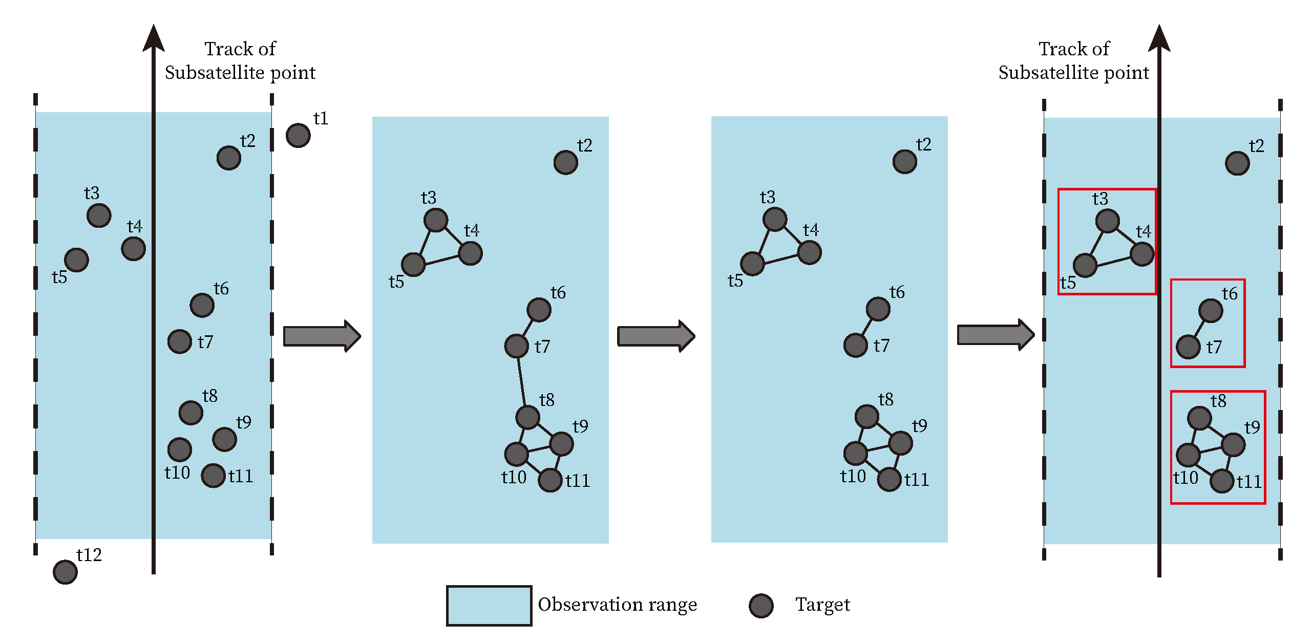
According to the constraints mentioned above, merged tasks need to be screened out, and the graph theory is used to build the clustering model. Firstly, we defined an undirected graph $G=\langle V,E\rangle$, where V is the set of vertexes and $V\left(G_i\right)$ represents all valid observation tasks in the $ith$ orbit, E is the set of edges and $E\left(G_i\right)$ denotes the links between two tasks. In the graph clustering model, any two original observation tasks with the edge connection satisfying the constraint conditions can be regarded as a clustering task. While expanding to a multiple vertex condition, multiple original tasks can be merged into one clustering task if there are edge connections between any two vertexes. The connected vertexes form a clique, where all vertexes are connected with each other, as shown in Figure 2, $\{t_3,t_4,t_5\}$, $\{t_6,t_7\}$ and $\{t_8,t_9,t_{1}0,t_{1}1\}$ can be seen as cliques and each clique is regarded as a clustering task.

In this paper, an adjacency matrix is adopted to better illustrate the utility of the graph clustering model. These original tasks $\{t_1,t_2,\cdots ,t_n\}$ can be described by a set of vertexes $V=\{v_1,v_2,\cdots ,v_n\}$ in the graph theory. Consequently, the graph clustering model could be represented by the adjacency matrix $A_{n\times n}$. If $t_u$ and $t_v$ meet the clustering constraint conditions, the relationship between two tasks can be described as $(v_u,v_v)\in E\left(G\right)$. Correspondingly, the element in the matrix $A_{uv}=1$, otherwise $A_{uv}=0$. Finally, the adjacency matrix $A_{n\times n}$ consisting of 0 and 1 forms the graph clustering model $E\left(G_i\right)$ in the $ith$ orbit.

2.2. Task Scheduling Problem

2.2.1. Scheduling Model

In this paper, a time-continuous resource allocation model for the EOSSP is established. Continuous decision variables are introduced to represent the observation start time within each VTW and decision variables are defined to check whether tasks are scheduled or not.

Figure 3 gives a task sequential execution description in one orbit, where $TWS$ and $TWE$ stand for the start and end time of the VTW of an observation task, respectively, d represents the observation duration time of a task, $tranT$ and s represent slewing angle maneuver time and preparation time, respectively, and $ObvS$ and $ObvE$ are the observation start time and end time.

2.2.2. Constraint Conditions

In this paper, the VTW is seen as the allocated resource, and the OWs for tasks are continuous decision variables to decide when to start the observation. The solution of the EOSSP model aims to schedule an observation sequence and maximize the observation profit, subject to corresponding constraints. In practical engineering scenarios, the following constraints are usually taken into account [24]:

(1) VTW constraint

The VTW constraint ensures that the observation tasks can be executed within the VTW of EOSs in the observation process.

For $\forall t_u^i\in \left\{t_i\mid i=1,2,\dots ,N\right\}$, where N is the number of tasks,

$$\left\{\begin{array}{c}Obv{S}_u^i\ge TW{S}_u^i\hfill \\ Obv{E}_u^i+d_u\le TW{E}_u^i\hfill \end{array}\right.$$

(6)

where $d_u$ represents the observation duration time of task $t_u$, $d_u=Obv{E}_u^i-Obv{S}_u^i$ is the observation start time of $t_u$ in the $ith$ orbit, $Obv{E}_u^i$ is defined as the observation end time. $TW{S}_u^i$ and $TW{E}_u^i$ represent the start and end time of the VTW for task $t_u^i$.

(2) Conflict constraint for task execution

The conflict constraint for task execution means that there is no crossover between any two tasks as the optical sensor cannot perform two observation tasks at the same time:

$$\sum _{v=1,v\ne u}^N{x}_{uv}\le 1$$

(7)

where $x_{uv}$ is a decision variable and denotes whether to transform execution from task $t_u$ to task $t_v$. $x_{uv}=1$ means that $t_v$ will be executed after $t_u$.

(3) Task conversion time constraint

Between any two sequential tasks, enough preparation time is required, mainly including slewing maneuvering time and sensor shutdown–restart setup time [38], which could be described as the following formula:

For $\forall u,v\in N$ and $u<v$,

$$Obv{S}_v^i-Obv{E}_u^i\ge s_{uv}+trans{T}_{uv}$$

(8)

where $s_{uv}$ is the preparation time for restarting the sensor and $tran{T}_{uv}$ is the slewing maneuver time from task $t_u$ to $t_v$, and the slewing maneuver time can be calculated as the following formula:

$$trans{T}_{uv}=\frac{\left|{\theta }_v-{\theta }_u\right|}{v_s}$$

(9)

In the above formula, ${\theta }_u$ and ${\theta }_v$ represent the observation slewing angle of $t_u$ and $t_v$. $v_s$ denotes the angular velocity of the satellite slewing maneuver.

(4) Optical sensor boot time constraint

According to the power constraint of the optical payload, the observation time of a task cannot exceed the maximum operating time of the optical sensor,

$$maxT\ge x_u{d}_u(u=1,2,\cdots ,N)$$

(10)

(5) Storage size constraint

Limited by the total storage size in the satellite, the constraint could be described as the following equation,

$$\sum _{u=1}^N{x}_u{c}_i{d}_u\le M$$

(11)

where M represents the total data storage capacity of the satellite in one orbit. $c_i$ is the storage consumption per unit observation time in one orbit.

(6) Power consumption constraint

In each orbit, the energy to be consumed is limited by the maximum capacity, and the corresponding energy consumed by the sensor operation and slewing maneuver is mainly considered in this paper as:

$$\sum _{u=1}^N{x}_u{e}_i{d}_u+\sum _{u=1}^N\sum _{v=1,v\ne u}^N{x}_{uv}\left(s_{uv}+tran{T}_{uv}\right){\epsilon }_{uv}\le E$$

(12)

In this formula, $e_i$ represents the energy consumption per unit time of observation operation. ${\epsilon }_{uv}$ represents the energy consumption per unit time of the slewing maneuver from $t_u$ to $t_v$. E is the total energy available for observation activities in one orbit.

2.2.3. Optimization Objectives

Models of observation satellite scheduling are always built as multiple objective optimization problems, and a scheduling algorithm aims to generate a compromise solution between objectives. Tangpattanakul et al. [39] implemented an indicator-based multi-objective local search method for the EOSSP, whose objectives were to maximize the total profit and simultaneously to ensure the fairness of resource allocation among multiple users. Sometimes, energy balance and fuel consumption are designed as optimization objectives [40,41].

In this paper, to maximize the total observation profit, more tasks and tasks with higher priority were scheduled. Hence, the objective function f was designed to maximize the total profit by the sum of priority associated with selected tasks.

$$f=max\left(\sum _{u=1}^N\frac{x_u}{N}pri{o}_u\right)$$

(13)

This optimization objective function is subject to the constraint model mentioned above.

3. Solving Method

3.1. Task Preprocess: Graph Clustering

In Section 2.1, we proposed an undirected graph clustering model $G=\langle V,E\rangle$. According to a previous analysis, clustering tasks can be selected by dividing the graph into independent cliques, aiming to minimize the number of clusters, which is known as the minimum clique partition algorithm [42]. Wu et al. [38,43] improved the clique partition algorithm by considering the priorities of vertices (original tasks) and adopted it in the task clustering phase. In this paper, an improved minimum clique partition algorithm is proposed. The maximum task priority and the minimum observation slewing angle of clustering tasks are taken into consideration simultaneously. This improvement could save energy to maintain a smaller observation slewing angle, which is significant in real engineering applications.

3.1.1. Graph Model Establishment

The establishment of a graph-based clustering model involves two steps, establishing the adjacency matrix and updating the model, as described below:

(1) Establish the adjacency matrix

All tasks in $V\left(G_i\right)$ are traversed and whether two original tasks $t_u$ and $t_v$ satisfy the time window constraint is checked. If the time window constraint is satisfied, $A_{uv}=1$, otherwise $A_{uv}=0$. After the iteration, the edge $(v_v,v_u)$ is generated, and the initial graph model $G_0$ is gained.

(2) Update graph model by checking other constraints

According to the initial graph $G_0$ built by satisfying the time window constraint, the adjacency matrix elements $A_{uv}(u,v=1,2,\cdots ,n)$ are searched. If $A_{uv}\ne 0$, constraints of the observation time window and observation slewing angle are checked sequentially. Once a constraint condition is not satisfied, $A_{uv}=0$. Finally, the clustering graph G and the adjacency matrix $A_{n\times n}$ are obtained.

3.1.2. Clique Partition Algorithm

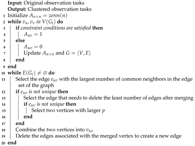
Based on the graph model, each independent cluster represents a clustering task. The purpose of the clique partition algorithm is to minimize the number of clustered tasks and ensuring more original tasks are contained in each divided clique. The algorithm is described as follows:

Firstly, the edge $e_{uv}$ with the largest number of common neighbors on the edge set $E\left(G_i\right)$ in the graph is selected. Secondly, the edge which needs to delete the least number of edges is screened out after merging. Thirdly, the edge which has a larger evaluation parameter p of the corresponding vertices is selected. Finally, the two vertices are merged into a new virtual vertex, and the edge associated with the merged vertex is deleted. Repeatedly applying the procedure to the updated edge set, the process is stopped when the original $E\left(G_i\right)$ becomes empty.

In the algorithm, evaluation parameter p can be calculated as follows:

$$pri{o}^c=\frac{1}{m}\left(pri{o}_1+pri{o}_2+\cdots +pri{o}_m\right)$$

(14)

$${\theta }^c=\frac{1}{2}\left(inf\left(\bigcap _{j=1}^m{\theta }_j\right)+sup\left(\bigcap _{j=1}^m{\theta }_j\right)\right)$$

(15)

$$p=\frac{pri{o}^c}{max\left(prio\right)}+\frac{max\theta }{{\theta }^c}$$

(16)

where $pri{o}^c$ and ${\theta }^c$ are the priority and the minimum slewing angle of the generated clustering task, respectively. The pseudocode of the improved minimum clique partition algorithm process is shown in Algorithm 1:

Algorithm 1: Improved minimum clique partition algorithm

In this paper, an improved clique partition algorithm is adopted by taking the priority and the minimum slewing angle of clustering tasks into consideration. The generated clustering tasks are used as the input of the following DRL algorithm to calculate the scheduling result.

3.2. DRL-Based Method for Optimization

3.2.1. Markov Decision Process Model

Deep reinforcement learning is the process of an agent that learns how to make a decision by interacting with the dynamic environment through trial and error. Agents take actions on the environment and achieve positive or negative reward feedback.

The Markov decision process (MDP) is the fundamental framework of RL for modeling. One agent (a satellite in this research) chooses an action in the current state, then transfers to the next state and receives a reward. This process could be described by a tuple $\mathcal{M}=\langle \mathcal{S},\mathcal{A},\mathcal{P},\mathcal{R},\gamma \rangle$, where $\mathcal{S}$ is a finite set of states, $\mathcal{A}$ is a finite set of actions, $\mathcal{P}$ is a state transition probability matrix. $\mathcal{R}$ represents the reward function and $\gamma$ denotes a discount factor ($\gamma \in [0,1]$).

In the EOSSP, the global state $\mathcal{S}$ includes the task state $S^{task}$ and the satellite state $S^{sat}$ is given as the following equations:

$$S^{task}=\bigcup _u^N\left[TW{S}_u^c,TW{E}_u^c,Obv{S}_u,Obv{E}_u,pri{o}_u,d_u\right]$$

(17)

$$S^{sat}=\bigcup _u^N{\theta }_u$$

(18)

where the global state $s_t=\mathcal{S}=[S^{task},S^{sat}]$. The task state $S^{task}$ is the collection of start and end times of the VTW, start and end times of the OW, priority and the observation duration. The satellite state $S^{sat}$ is the collection of observation slewing angles.

The action space $\mathcal{A}$ is the collection of decision variables of each task, and all of the value range is normalized to $[-1,1]$ as follows:

$$\mathcal{A}=\bigcup _u^N{a}_u(a\in [-1,1])$$

(19)

It should be noted that $\mathcal{A}$ is not the OW for each task, and the corresponding mapping function is given in the following equation.

$$\left\{\begin{array}{c}Obv{S}_u=TW{S}_u+\frac{a_u+1}{2}\left(TW{E}_u-TW{S}_u\right)\hfill \\ Obv{E}_u=Obv{S}_u+d_u\hfill \end{array}\right.$$

(20)

The selected OW for task $t_u$ is $[Obv{S}_u,Obv{E}_u]$ and could be seen as the global solution for the EOSSP. It is noted that in a model-free algorithm, it does not need any hypothesis or a prior knowledge P. The VTW-related state $s_t$ will transform to the next state $s_{t+1}$ after an OW-related action $a_t$ occurs. This process happens continuously within a finite time, and an immediate reward $r_t$ is obtained predictably in each transition step, as shown in Figure 4.

3.2.2. Optimization with DDPG

In 2015, Mnih et al. [44] proposed the first successful deep Q-network (DQN) frame in Atari games, with the main idea of mapping the state to action-value function by deep networks. However, the action taken is given by $a_t=argmaxQ(s_t,a)$, which means the DQN could handle discrete action space problems. In the optimization research domain, in terms of the TSP model or VRP model problems, the agent is designed to make sequential discrete decisions, and the DQN has been applied successfully [27,28,29].

COntrary to the DQN, the main idea of the DDPG is mapping state to policy (specific actions taken) directly. Therefore the DDPG could make continuous decision variables and has advantages in large-dimensional problems [45]. In this paper, the EOSSP is modeled as a time-continuous resource allocation problem, where the VTW is the crucial resource. The policy made is to decide a specific time for each observation task, and the action space is typically continuous, so it is suitable for the DDPG solution.

The DDPG algorithm conforms to the actor–critic framework, which includes the actor network and critic network. The actor network is represented by parameters ${\theta }_{\mu }$, which offers a strategy action distribution according to the current state. The critic network evaluates the current strategy by calculating the value function and its parameters are denoted by ${\theta }_q$.

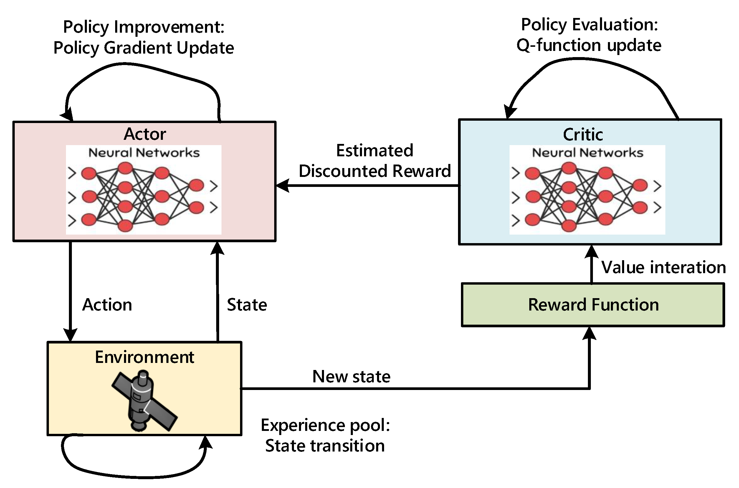
Figure 5 illustrates the DDPG algorithm. The actor network outputs an action from a continuous action space, which converts the state space into the action $a=\mu \left(s\right)$. In the critic network, the output $Q(s,\mu (s\left)\right)$ is learned by using the Bellman equation, which represents the approximation of the discounted total reward. In every step of the optimization training process, the actor network is improved by computing the gradient of the $Q(s,\mu (s\left)\right)$ function, which could be calculated by applying the chain rule [45]:

$$\nabla Q(s,\mu \left(s\right))\approx {\nabla }_{a}Q(s,a){\nabla }_{{\theta }_{\mu }}\mu \left(s\right)$$

(21)

In order to ensure the scheduling network convergence, target networks are adopted to update parameters periodically. Correspondingly, ${\theta }_{\mu }^{\prime }$ and ${\theta }_q^{\prime }$ are defined to represent parameters of the target actor network and the target critic network.

3.2.3. Task Scheduling Method

As an off-policy DRL algorithm, the DDPG allows us to train the EOS task scheduling network without knowing the prior information. Moreover, it is noted that in the training process, valid observation tasks are sorted according to the start time of the VTW.

(1) Network architecture

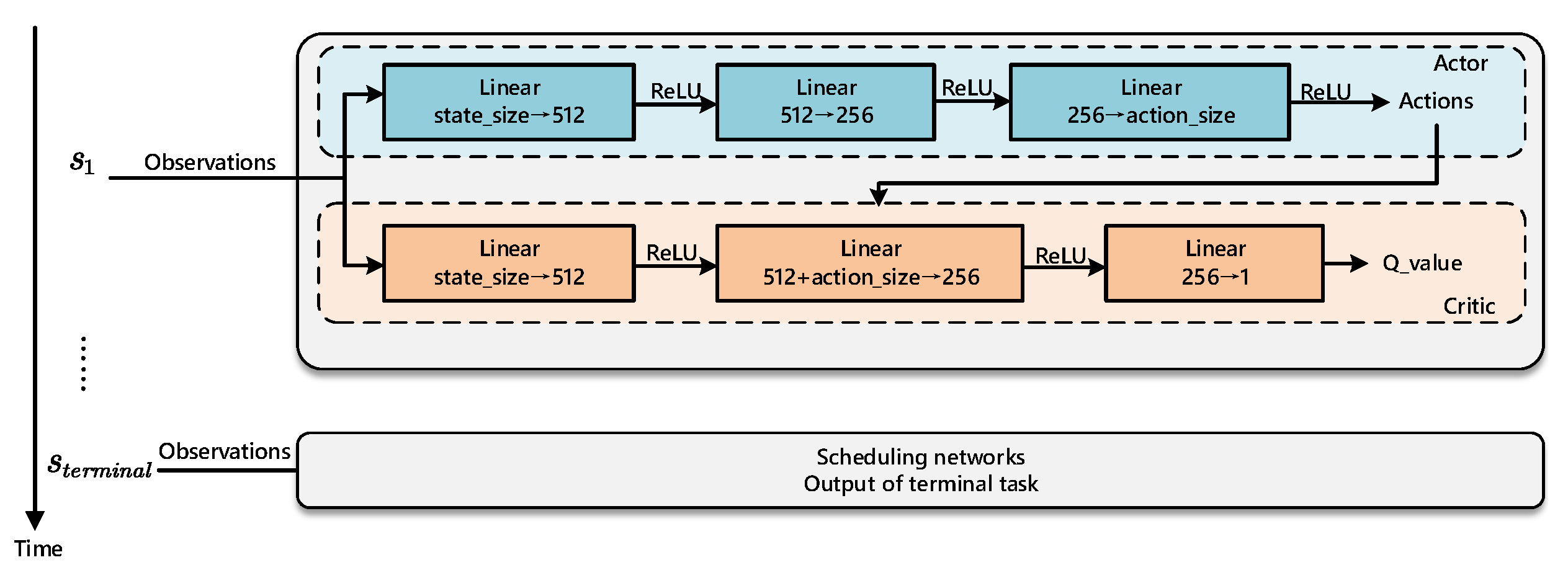
As mentioned above, the model consists of two separate networks, which are, respectively, the actor and the critic. Figure 6 shows the network architecture.

The input of the network is a sequence of state information (denoted as s), including the start and end time of the VTW, start and end time of the OW, priority and the observation duration. The L2-normalization is applied to the state input layer and the output of the architecture has two parts: an estimation Q-value of total expected profit (denoted as $Q(s,a\mid {\theta }_q$)) as critic and the policy (denoted as $\mu (s\mid {\theta }_{\mu }$)) for the task as actor. The output value of the actor network is mapped to $[-1,1]$ by applying a non-linear activation function $Tanh$, which has the same value range as the action space in Equation (19).

$$Tanh\left(x\right)=\frac{e^x-e^{-x}}{e^x+e^{-x}}$$

(22)

(2) Reward function design

In the task scheduling problem, the EOS must guarantee that high-priority observation tasks in the execution sequence can be carried out. Simultaneously, to meet actual requirements, conflicting tasks are not permitted. Therefore, the reward function, denoted by $r_t$, is modeled to supervise the task scheduler to achieve an optimal result. In Section 2.2, we propose the optimization objective function f in Equation (13). Thus, to acquire the largest global profit, the reward function is formulated as follows:

$$r_t=r(s_t,a_t)=\lambda (f_t-f_{t-1})$$

(23)

where $\lambda$ is an amplification factor to improve a good action’s reward and accelerate the process of training the policy network.

(3) Training method

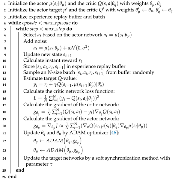
In the training process, the scheduling network makes a decision when to start observing targets, and then receives an instant reward based on the reward function. For considering the future reward given by the current policy, an accumulated reward with a discount factor $\gamma$ is used to estimate the Q-value in the critic network. Meanwhile, the actor could learn to make an optimal scheduling policy based on the actor network. During each training step, the critic improves its prediction ability by gradient descent of error between actual profit and estimated profit. The actor updates its parameters based on the prediction from the critic. To improve exploration efficiency, noise is introduced into the decision as follows:

$$a_t=\mu (s_t\mid {\theta }_{\mu })+\alpha \mathcal{N}(0,{\sigma }^2)$$

(24)

The noise obeys the normal distribution and $\alpha$ is the attenuation coefficient, $\sigma$ is the standard deviation. At the end of each training episode, a soft synchronization method is adopted to update network parameters, which is formulated as follows:

$$\left\{\begin{array}{c}{\theta }_{\mu }^{\prime }=\tau {\theta }_{\mu }+(1-\tau ){\theta }_{\mu }^{\prime }\hfill \\ {\theta }_q^{\prime }=\tau {\theta }_q+(1-\tau ){\theta }_q^{\prime }\hfill \end{array}\right.$$

(25)

where $\tau$ is the coefficient of synchronization, which is used to make the target networks slowly track the learned networks, significantly improving the stability of learning [45]. The pseudocode for the scheduling algorithm is shown in Algorithm 2:

Algorithm 2: Task scheduling method based on DDPG

(4) Resolving conflicts

After the OW is determined by the DDPG, conflicts may still remain. Constraint checking and conflict resolving are performed, and the breadth first search (BFS) is adopted to check the task sequence and update the list $\{x_1,x_2,\dots ,x_N\}$ to $\{0,1,1,0,\cdots \}$. After resolving conflicts, the profit obtained in the current step is calculated according to Equation (13).

4. Experimental Simulation

4.1. Simulation Scenario

In this paper, a typical engineering scenario is taken into consideration, where the observation targets were generated randomly with different task numbers in the region between ${40}^{\circ }$ and ${45}^{\circ }$ (N) latitude and ${117}^{\circ }$ and ${130}^{\circ }$ (E) longitude, as shown in Figure 7. The simulation scenario was implemented by using the System Tool Kit (STK) and six typical orbital elements of an LEO observation satellite are selected, as listed in

Table 2. Orbital element settings.

Parameters	Value
Semi-major axis of orbit a	7000 km
Orbital eccentricity e	0
Orbital inclination i	${60}^{\circ }$
Longitude of ascending node $\mathrm{\Omega }$	${285}^{\circ }$
Argument of perihelion $\omega$	$0^{\circ }$
Mean anomaly $M_0$	$0^{\circ }$

.

In addition, 50, 100, 150 and 200 original tasks were generated to simulate practical users’ requests. In addition, different task numbers represent the increasing complexity of the EOSSP. In the comparison experiment groups, the performance and scalability of the proposed DDPG algorithm were validated and discussed while the problem scale increased.

The resource-related constraints, including the VTW, slewing angle maneuverability, total energy, total memory constraints, etc., were taken into account, and associated constant variables are summarized in

Table 3. Constraint conditions in the task scheduling.

Parameters	Value	Parameters	Value
M	600	$c_i$	1
$FOV$	${10}^{\circ }$	$e_i$	1
$maxT$	150 s	${\epsilon }_{uv}$	0.5
$max\theta$	$\pm {40}^{\circ }$	E	1200

.

It is emphasized that tasks waiting to be scheduled were arranged in chronological order according to the start time of the VTW. Meanwhile, tasks were set up with different observation durations, ranging from 5 s to 15 s, and different priorities, ranging from 1 to 10.

4.2. Results and Discussion

According to the analysis in Section 3, task clustering is an effective approach promoting scheduling efficiency and saving EOS resources. For the task clustering preprocess phase, the proposed minimum clique partitioning algorithm consists of two steps. Firstly, it establishes the clustering graph by considering constraint conditions, and then it partitions original tasks into minimum clique aiming to update the task execution sequence. Figure 8 shows the clique partition result of 50 original tasks, where $\{t_1,t_2,t_3,t_4\}$ are inaccessible. The interconnected vertexes such as $\{t_{29},t_{34},t_{37}\}$ can be seen as a merged task.

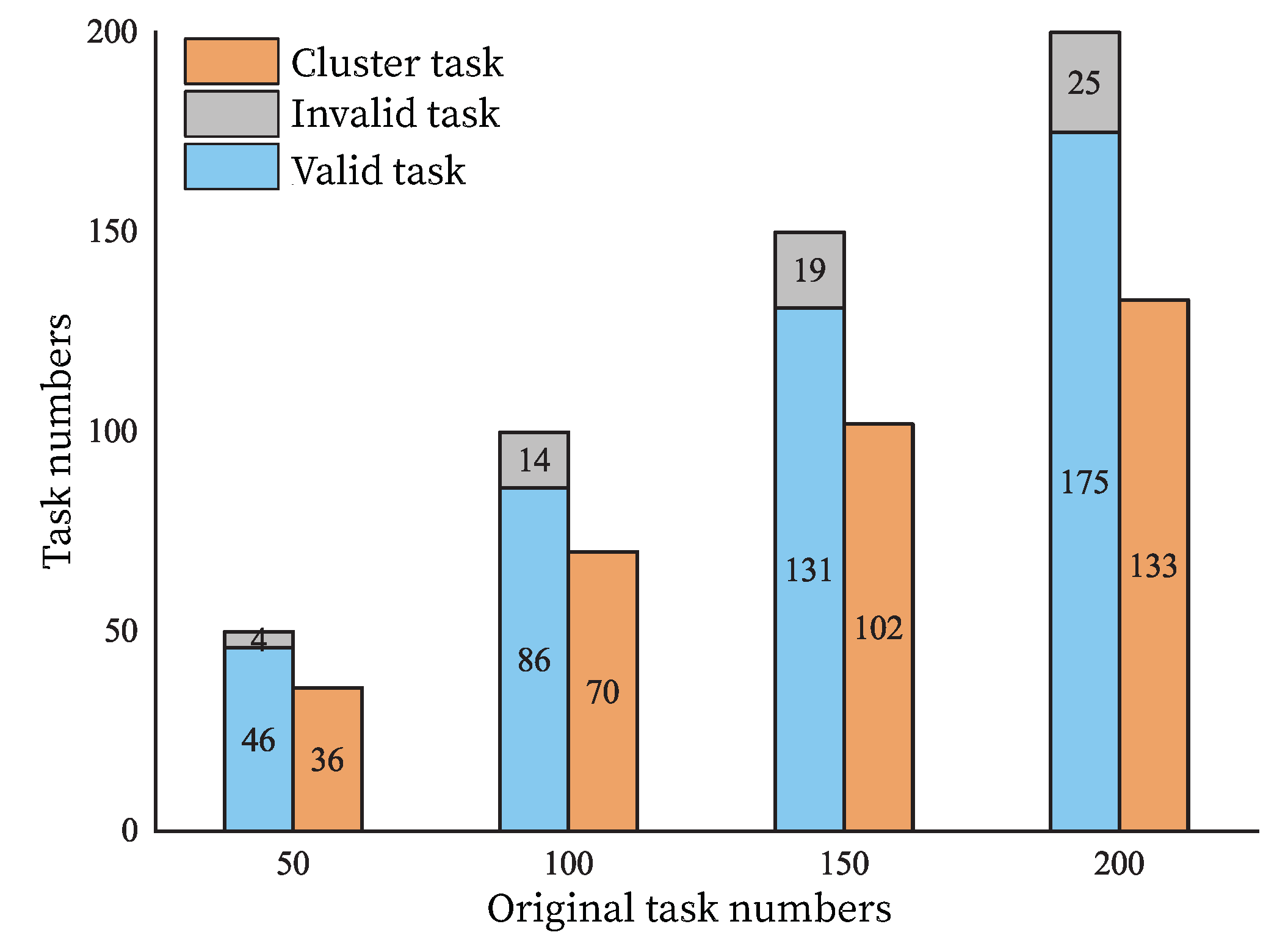
Furthermore, other groups of comparisons with 100, 150 and 200 original tasks were simulated, as shown in Figure 9. The results indicate that 4, 14, 19 and 25 corresponding invalid tasks are eliminated and 36, 70, 102 and 133 clustering tasks are generated. Moreover, it is found that the task clustering running time is less than 0.5 s. Thus, it could be stated that the improved graph-based minimum clique partition algorithm achieves the desired objective and reduces the task scale obviously and quickly.

On the basis of the results from the clustering, the performance of the RL-based algorithm is examined, where the Pytorch deep learning framework is utilized to implement the scheduling networks.

Table 4. Training hyperparameter settings.

Parameters	Value
Learning rate for the critic	0.002
Learning rate for the actor	0.001
Discount factor $\gamma$	0.95
Memory capacity	3000
Batch size	32
Noise attenuation coefficient $\alpha$	0.9995
Standard deviation $\sigma$	0.1
Soft synchronization coefficient $\tau$	0.001

gives the hyperparameters adopted in the training process.

The DRL algorithm runs on an Nvidia GTX1660 GPU and Intel i5-8400 CPU device. In each training episode, there are 100 exploratory steps, and the maximum training episode is 400, which means the total amount of experience is 40,000. The experience memory pool keeps updated data with a size of 3000. In each training step, experiences are randomly sampled from the memory pool with a batch size of 32. Parameters of the actor and the critic networks are initialized randomly before training, and the models are trained with the ADAM optimizer [46].

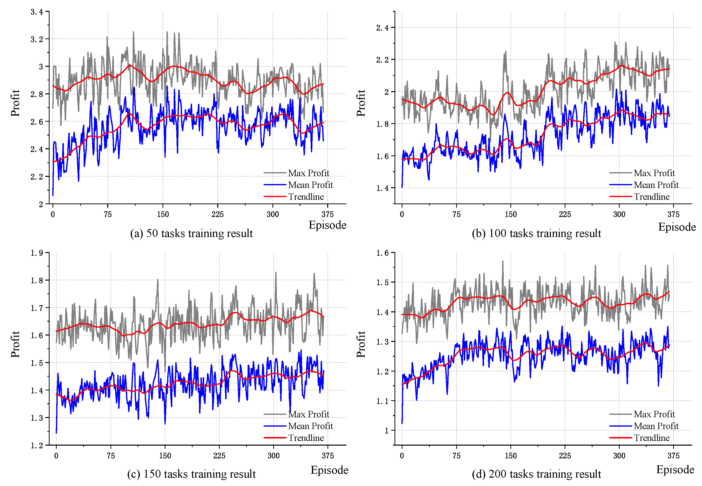
The task scheduling profit p proposed in Section 2.2 is selected as the evaluation indexes of the training performance. As shown in Figure 10 the episode maximum profit (gray curves) and average profit (blue curves) are selected to demonstrate the algorithm’s performance in each training episode. The trendline (red curves) indicates that the task scheduling network could achieve a higher profit in every simulation, which demonstrates that the proposed method is working. The profit score of scheduling is fluctuates upward with increasing episodes, which shows that the network could learn from experience and achieve a better and more stable scheduling policy with higher profit.

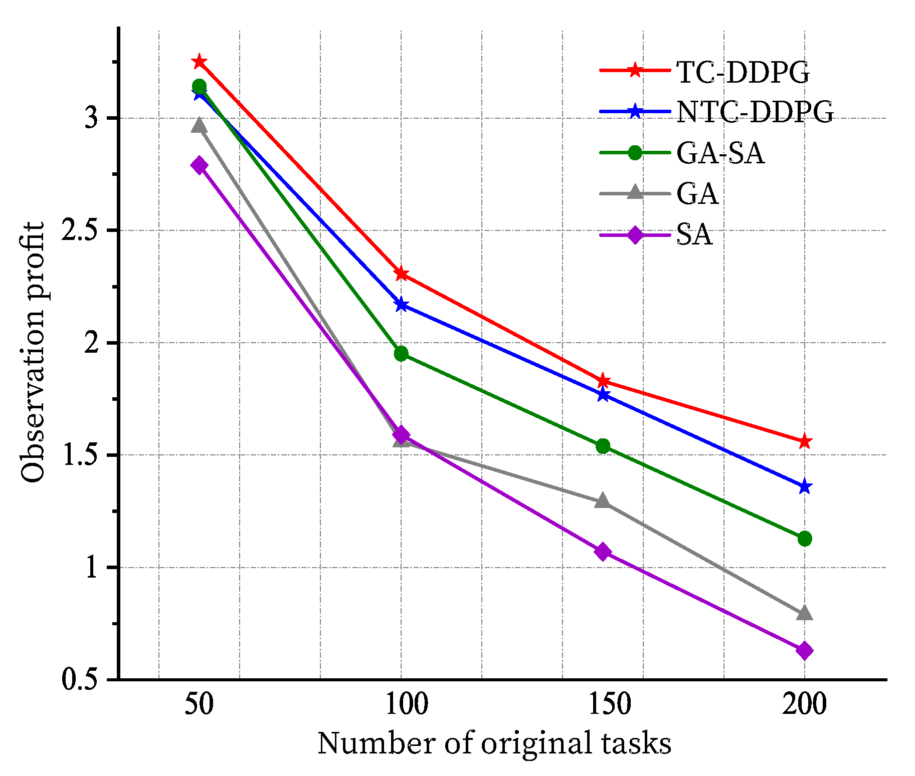
Additionally, the trained DRL scheduling network gives a solution with observation profit of 3.25 for 50 original tasks, but the profit of allocating 100, 150 and 200 original tasks decreases it to 2.31, 1.83 and 1.56, respectively. Therefore, the desired profit is greatly influenced by the number of original tasks, representing the complexity of the EOSSP. The main possible reason for this is that the observation tasks are under the limitation of the VTW, energy, storage and other constraint conditions, and task scheduling becomes more and more difficult while the number of tasks increases. A compromising solution is to ensure tasks with higher priority are executed.

Figure 11 demonstrates the observation time period selection of the DDPG methods in the task scheduling phase for 50 original tasks. The horizontal axis represents the time and the vertical axis represents different clustered observation tasks. The left figure shows the initial state, where all tasks are arranged at the start of the VTW. The scheduling result is shown in the right figure, where valid tasks (marked as green) are executed, and the invalid tasks (marked as red) are not performed because of constraint conflicts.

Moreover, a series of comparisons with the genetic algorithm (GA), the simulated annealing algorithm (SA) and the GA–SA hybrid algorithm is performed to examine the superiority of the DDPG method. Note that the GA–SA hybrid algorithm has been validated in our previous work [24]. In addition, the DDPG without considering the task clustering is simulated to withstand the effect of the preprocess, and it is defined as NTC-DDPG. Correspondingly, the DDPG with task clustering is represented by TC-DDPG.

Comparison results are given in Figure 12. It is indicated that the TC-DDPG method always gives a good optimization result compared with other methods. Interestingly, it was found that for 50 tasks, NTC-DDPG has a relatively low profit, but with the increase in the task number, NTC-DDPG exceeds the non-DRL methods, even though NTC-DDPG does not take the task clustering into account. This indicates that the DDPG could contribute to a high EOS efficiency. It is necessary to point out that the non-DRL methods also include the task clustering preprocess.

Additionally, it is obvious that traditional optimization algorithms achieve a worse profit with the increases in the number of original tasks, and the SA algorithm is even out of work in the 150 and 200 task-scale situations. Hence, the DRL method has practical advantages when addressing a large-scale EOSSP. The results shown in

Table 5. Algorithm performance comparison.

	Profit				Running Time (s)
Task Numbers	50	100	150	200	50	100	150	200
TC-DDPG	3.25	2.31	1.83	1.56	163.7	228.3	295.3	362.4
NTC-DDPG	3.11	2.17	1.77	1.36	181.1	255.2	352.1	454.7
GA-SA	3.14	1.95	1.54	1.13	155.3	163.7	362.9	530.2
GA	2.96	1.56	1.29	0.79	3.7	6.4	10.3	15.6
SA	2.79	1.59	1.07	0.63	47.1	83.4	379.2	702.3

illustrate the feasibility of the proposed RL method and this method is rather competitive in the EOSSP, with good profit performance and adaptability to practical applications. In addition, the task clustering algorithm greatly improves the DDPG algorithm, obtaining a higher observation profit and reducing the running time, with a preprocess time of less than 0.5 s.

5. Conclusions

Observation satellite task scheduling policy plays a crucial role in providing high-quality space-based information services. In previous studies, many algorithms based on traditional optimization methods such as GA and SA have been successfully applied in the EOSSP. However, these methods depend upon a mathematical model, and with the increase in the task scale, they may fall into local optimum. In this paper, the EOSSP is considered as a time-continuous model with multiple constraints and, inspired by the progress of DRL and its model-free characteristics, a DRL-based algorithm is proposed to approach the EOSSP. In addition, to decrease the complexity of the solution, an improved graph-based minimum clique partition algorithm is proposed for the task clustering preprocess; this is a relatively new attempt in handling EOSSP optimization. The simulation results show that the DDPG algorithm combined with the task clustering process is practicable and achieves the expected performance. In addition, this solution has a higher optimization performance compared with traditional metaheuristic algorithms (GA, SA and GA–SA hybrid algorithm). In terms of scheduling profits, the experimental results indicate that the DDPG is feasible and efficient for the EOSSP even in a relatively large-scale situation.

Note that, in the present work, satellite constellation task scheduling problems were not addressed. In a future study, we will attempt to adopt multi-agent DRL methods to study the multiple satellite EOSSP.

References

1. Bianchessi, N.; Cordeau, J.F.; Desrosiers, J.; Laporte, G.; Raymond, V. A Heuristic for the Multi-Satellite, Multi-Orbit and Multi-User Management of Earth Observation Satellites. Eur. J. Oper. Res. 2007, 177, 750–762. [Google Scholar] [CrossRef]
2. Bianchessi, N.; Righini, G. Planning and Scheduling Algorithms for the COSMO-SkyMed Constellation. Aerosp. Sci. Technol. 2008, 12, 535–544. [Google Scholar] [CrossRef]
3. Irrgang, C.; Saynisch, J.; Thomas, M. Estimating Global Ocean Heat Content from Tidal Magnetic Satellite Observations. Sci. Rep. 2019, 9, 1–8. [Google Scholar]
4. Gevaert, C.M.; Suomalainen, J.; Tang, J.; Kooistra, L. Generation of Spectral–Temporal Response Surfaces by Combining Multispectral Satellite and Hyperspectral UAV Imagery for Precision Agriculture Applications. IEEE J. Sel. Top. Appl. Earth Obs. Remote. Sens. 2015, 8, 3140–3146. [Google Scholar] [CrossRef]
5. Lemaître, M.; Verfaillie, G.; Jouhaud, F.; Lachiver, J.M.; Bataille, N. Selecting and Scheduling Observations of Agile Satellites. Aerosp. Sci. Technol. 2002, 6, 367–381. [Google Scholar] [CrossRef]
6. Zheng, Z.; Guo, J.; Gill, E. Distributed Onboard Mission Planning for Multi-Satellite Systems. Aerosp. Sci. Technol. 2019, 89, 111–122. [Google Scholar] [CrossRef]
7. Wang, X.; Wu, G.; Xing, L.; Pedrycz, W. Agile Earth Observation Satellite Scheduling over 20 Years: Formulations, Methods, and Future Directions. IEEE Syst. J. 2020. [Google Scholar] [CrossRef]
8. Xu, R.; Wang, H.; Zhu, S.; Jiang, H.; Li, Z. Multiobjective Planning for Spacecraft Reorientation under Complex Pointing Constraints. Aerosp. Sci. Technol. 2020, 104, 106002. [Google Scholar] [CrossRef]
9. Wolfe, W.J.; Sorensen, S.E. Three Scheduling Algorithms Applied to the Earth Observing Systems Domain. Manag. Sci. 2000, 46, 148–166. [Google Scholar] [CrossRef]
10. Zhu, X.; Zhang, C.; Sun, R.; Chen, J.; Wan, X. Orbit Determination for Fuel Station in Multiple SSO Spacecraft Refueling Considering the J2 Perturbation. Aerosp. Sci. Technol. 2020, 105, 105994. [Google Scholar] [CrossRef]
11. Chen, X.; Reinelt, G.; Dai, G.; Spitz, A. A Mixed Integer Linear Programming Model for Multi-Satellite Scheduling. Eur. J. Oper. Res. 2019, 275, 694–707. [Google Scholar] [CrossRef] [Green Version]
12. Peng, G.; Dewil, R.; Verbeeck, C.; Gunawan, A.; Xing, L.; Vansteenwegen, P. Agile Earth Observation Satellite Scheduling: An Orienteering Problem with Time-Dependent Profits and Travel Times. Comput. Oper. Res. 2019, 111, 84–98. [Google Scholar] [CrossRef]
13. Liu, X.; Laporte, G.; Chen, Y.; He, R. An Adaptive Large Neighborhood Search Metaheuristic for Agile Satellite Scheduling with Time-Dependent Transition Time. Comput. Oper. Res. 2017, 86, 41–53. [Google Scholar] [CrossRef]
14. Wang, X.W.; Chen, Z.; Han, C. Scheduling for Single Agile Satellite, Redundant Targets Problem Using Complex Networks Theory. Chaos Solitons Fractals 2016, 83, 125–132. [Google Scholar] [CrossRef]
15. Valicka, C.G.; Garcia, D.; Staid, A.; Watson, J.P.; Hackebeil, G.; Rathinam, S.; Ntaimo, L. Mixed-Integer Programming Models for Optimal Constellation Scheduling given Cloud Cover Uncertainty. Eur. J. Oper. Res. 2019, 275, 431–445. [Google Scholar] [CrossRef]
16. Wang, X.; Han, C.; Zhang, R.; Gu, Y. Scheduling Multiple Agile Earth Observation Satellites for Oversubscribed Targets Using Complex Networks Theory. IEEE Access 2019, 7, 110605–110615. [Google Scholar] [CrossRef]
17. Islas, M.A.; Rubio, J.d.J.; Muñiz, S.; Ochoa, G.; Pacheco, J.; Meda-Campaña, J.A.; Mujica-Vargas, D.; Aguilar-Ibañez, C.; Gutierrez, G.J.; Zacarias, A. A Fuzzy Logic Model for Hourly Electrical Power Demand Modeling. Electronics 2021, 10, 448. [Google Scholar] [CrossRef]
18. De Jesus Rubio, J. SOFMLS: Online Self-Organizing Fuzzy Modified Least-Squares Network. IEEE Trans. Fuzzy Syst. 2009, 17, 1296–1309. [Google Scholar] [CrossRef]
19. Gabrel, V.; Moulet, A.; Murat, C.; Paschos, V.T. A New Single Model and Derived Algorithms for the Satellite Shot Planning Problem Using Graph Theory Concepts. Ann. Oper. Res. 1997, 69, 115–134. [Google Scholar] [CrossRef]
20. Jang, J.; Choi, J.; Bae, H.J.; Choi, I.C. Image Collection Planning for KOrea Multi-Purpose SATellite-2. Eur. J. Oper. Res. 2013, 230, 190–199. [Google Scholar] [CrossRef]
21. Liu, S.; Yang, J. A Satellite Task Planning Algorithm Based on a Symmetric Recurrent Neural Network. Symmetry 2019, 11, 1373. [Google Scholar] [CrossRef] [Green Version]
22. Kim, H.; Chang, Y.K. Mission Scheduling Optimization of SAR Satellite Constellation for Minimizing System Response Time. Aerosp. Sci. Technol. 2015, 40, 17–32. [Google Scholar] [CrossRef]
23. Niu, X.; Tang, H.; Wu, L. Satellite Scheduling of Large Areal Tasks for Rapid Response to Natural Disaster Using a Multi-Objective Genetic Algorithm. Int. J. Disaster Risk Reduct. 2018, 28, 813–825. [Google Scholar] [CrossRef]
24. Long, X.; Wu, S.; Wu, X.; Huang, Y.; Mu, Z. A GA-SA Hybrid Planning Algorithm Combined with Improved Clustering for LEO Observation Satellite Missions. Algorithms 2019, 12, 231. [Google Scholar] [CrossRef] [Green Version]
25. Mao, H.; Alizadeh, M.; Menache, I.; Kandula, S. Resource Management with Deep Reinforcement Learning. In Proceedings of the 15th ACM Workshop on Hot Topics in Networks; Association for Computing Machinery: Atlanta, GA, USA, 2016; pp. 50–56. [Google Scholar]
26. Sutton, R.S.; McAllester, D.A.; Singh, S.P.; Mansour, Y. Policy Gradient Methods for Reinforcement Learning with Function Approximation. Adv. Neural Inf. Process. Syst. 1999, 99, 1057–1063. [Google Scholar]
27. Bello, I.; Pham, H.; Le, Q.V.; Norouzi, M.; Bengio, S. Neural Combinatorial Optimization with Reinforcement Learning. arXiv 2016, arXiv:1611.09940. [Google Scholar]
28. Khalil, E.; Dai, H.; Zhang, Y.; Dilkina, B.; Song, L. Learning Combinatorial Optimization Algorithms over Graphs. Adv. Neural Inf. Process. Syst. 2017, 30, 6348–6358. [Google Scholar]
29. Nazari, M.; Oroojlooy, A.; Snyder, L.; Takác, M. Reinforcement Learning for Solving the Vehicle Routing Problem. Adv. Neural Inf. Process. Syst. 2018, 31, 9839–9849. [Google Scholar]
30. Peng, B.; Wang, J.; Zhang, Z. A Deep Reinforcement Learning Algorithm Using Dynamic Attention Model for Vehicle Routing Problems. In International Symposium on Intelligence Computation and Applications; Springer: Singapore, 2019; pp. 636–650. [Google Scholar]
31. Khadilkar, H. A Scalable Reinforcement Learning Algorithm for Scheduling Railway Lines. IEEE Trans. Intell. Transp. Syst. 2018, 20, 727–736. [Google Scholar] [CrossRef]
32. Ye, H.; Li, G.Y.; Juang, B.H.F. Deep Reinforcement Learning Based Resource Allocation for V2V Communications. IEEE Trans. Veh. Technol. 2019, 68, 3163–3173. [Google Scholar] [CrossRef] [Green Version]
33. Hadj-Salah, A.; Verdier, R.; Caron, C.; Picard, M.; Capelle, M. Schedule Earth Observation Satellites with Deep Reinforcement Learning. arXiv 2019, arXiv:1911.05696. [Google Scholar]
34. Haijiao, W.; Zhen, Y.; Wugen, Z.; Dalin, L. Online Scheduling of Image Satellites Based on Neural Networks and Deep Reinforcement Learning. Chin. J. Aeronaut. 2019, 32, 1011–1019. [Google Scholar]
35. Zhao, X.; Wang, Z.; Zheng, G. Two-Phase Neural Combinatorial Optimization with Reinforcement Learning for Agile Satellite Scheduling. J. Aerosp. Inf. Syst. 2020, 17, 346–357. [Google Scholar] [CrossRef]
36. Lam, J.T.; Rivest, F.; Berger, J. Deep Reinforcement Learning for Multi-Satellite Collection Scheduling. In International Conference on Theory and Practice of Natural Computing; Springer: Cham, Switzerland, 2019; pp. 184–196. [Google Scholar]
37. Wu, G.; Du, X.; Fan, M.; Wang, J.; Shi, J.; Wang, X. Ensemble of Heuristic and Exact Algorithm Based on the Divide and Conquer Framework for Multi-Satellite Observation Scheduling. arXiv 2020, arXiv:2007.03644. [Google Scholar]
38. Wu, G.; Liu, J.; Ma, M.; Qiu, D. A Two-Phase Scheduling Method with the Consideration of Task Clustering for Earth Observing Satellites. Comput. Oper. Res. 2013, 40, 1884–1894. [Google Scholar] [CrossRef]
39. Tangpattanakul, P.; Jozefowiez, N.; Lopez, P. A Multi-Objective Local Search Heuristic for Scheduling Earth Observations Taken by an Agile Satellite. Eur. J. Oper. Res. 2015, 245, 542–554. [Google Scholar] [CrossRef] [Green Version]
40. Wang, S.; Zhao, L.; Cheng, J.; Zhou, J.; Wang, Y. Task Scheduling and Attitude Planning for Agile Earth Observation Satellite with Intensive Tasks. Aerosp. Sci. Technol. 2019, 90, 23–33. [Google Scholar] [CrossRef]
41. Liu, F.; Gao, F.; Zhang, W.; Zhang, B.; He, J. The Optimization Design with Minimum Power for Variable Speed Control Moment Gyroscopes with Integrated Power and Attitude Control. Aerosp. Sci. Technol. 2019, 88, 287–297. [Google Scholar] [CrossRef]
42. Tseng, C.; Siewiorek, D.P. Automated Synthesis of Data Paths in Digital Systems. IEEE Trans. Comput. Aided Des. Integr. Circ. Syst. 1986, 5, 379–395. [Google Scholar] [CrossRef]
43. Wu, G.; Wang, H.; Pedrycz, W.; Li, H.; Wang, L. Satellite Observation Scheduling with a Novel Adaptive Simulated Annealing Algorithm and a Dynamic Task Clustering Strategy. Comput. Ind. Eng. 2017, 113, 576–588. [Google Scholar] [CrossRef]
44. Mnih, V.; Kavukcuoglu, K.; Silver, D.; Rusu, A.A.; Veness, J.; Bellemare, M.G.; Graves, A.; Riedmiller, M.; Fidjeland, A.K.; Ostrovski, G.; et al. Human-Level Control through Deep Reinforcement Learning. Nature 2015, 518, 529–533. [Google Scholar] [CrossRef]
45. Lillicrap, T.P.; Hunt, J.J.; Pritzel, A.; Heess, N.; Erez, T.; Tassa, Y.; Silver, D.; Wierstra, D. Continuous Control with Deep Reinforcement Learning. arXiv 2015, arXiv:1509.02971. [Google Scholar]
46. Kingma, D.P.; Ba, J. Adam: A Method for Stochastic Optimization. arXiv 2014, arXiv:1412.6980. [Google Scholar]
Figure 1. EOS observes targets in orbit.
Remotesensing 13 02377 g001
Figure 2. Illustration of clique partition for clustering graph.
Remotesensing 13 02377 g002
Figure 3. Description of the observation task scheduling sequence.
Remotesensing 13 02377 g003
Figure 4. Markov decision process in EOSSP.
Remotesensing 13 02377 g004
Figure 5. Illustration of DDPG algorithm.
Remotesensing 13 02377 g005
Figure 6. Architecture of DDPG actor and critic network.
Remotesensing 13 02377 g006
Figure 7. Observation target point map.
Remotesensing 13 02377 g007
Figure 8. Result of the minimum task clique partition.
Remotesensing 13 02377 g008
Figure 9. Performance demonstration of clustering algorithm.
Remotesensing 13 02377 g009
Figure 10. Profit curves of training performance.
Remotesensing 13 02377 g010
Figure 11. Observation time period selection results.
Remotesensing 13 02377 g011
Figure 12. Optimization performance contrast.
Remotesensing 13 02377 g012