Microphysical Characteristics of Rainfall Observed by a 2DVD Disdrometer during Different Seasons in Beijing, China

Abstract

The seasonal variations of raindrop size distribution (DSD) and rainfall are investigated using three-year (2016–2018) observations from a two-dimensional video disdrometer (2DVD) located at a suburban station (40.13° N, 116.62° E, ~30 m AMSL) in Beijing, China. The annual distribution of rainfall presents a unimodal distribution with a peak in summer with total rainfall of 966.6 mm, followed by fall. Rain rate (R), mass-weighted mean diameter (D_m), and raindrop concentration (N_t) are stratified into six regimes to study their seasonal variation and relative rainfall contribution to the total seasonal rainfall. Heavy drizzle/light rain (R2: 0.2~2.5 mm h⁻¹) has the maximum occurrence frequency throughout the year, while the total rainfall in summer is primarily from heavy rain (R4: 10~50 mm h⁻¹). The rainfall for all seasons is contributed primarily from small raindrops (D_m2: 1.0~2.0 mm). The distribution of occurrence frequency of N_t and the relative rainfall contribution exhibit similar behavior during four seasons with N_t of 10~1000 m⁻³ registering the maximum occurrence and rainfall contributions. Rainfall in Beijing is dominated by stratiform rain (SR) throughout the year. There is no convective rainfall (CR) in winter, i.e., it occurs most often during summer. DSD of SR has minor seasonal differences, but varies significantly in CR. The mean values of log₁₀N_w (N_w: mm⁻¹m⁻³, the generalized intercept parameter) and D_m of CR indicate that the CR during spring and fall in Beijing is neither continental nor maritime, at the same time, the CR in summer is close to the maritime-like cluster. The radar reflectivity (Z) and rain rate (𝑅) relationship (Z = 𝑎R^𝑏) showed seasonal differences, but were close to the standard NEXRAD Z-R relationship in summer. The shape of raindrops observed from 2DVD was more spherical than the shape obtained from previous experiments, and the effect of different axis ratio relations on polarimetric radar measurements was investigated through T-matrix-based scattering simulations.

1. Introduction

The microphysical process of cloud and precipitation plays an essential role in the formation and evolution of rainfall. Many studies concentrated on microscopic cloud physics have shown that considerable differences in the intensity and distribution of rain can reveal the different microphysical properties of clouds [1,2]. The space and time variation of raindrop size distribution (DSD) within an observation area is related to a series of microphysical processes, such as condensation, coalescence, freezing, attachment, melting, fragmentation, and evaporation of particles in a particular precipitation system [3]. Therefore, the knowledge of DSD is not only helpful to understand the precipitation microphysics [4] and establish the radar quantitative precipitation estimation (QPE) algorithms [5,6,7], but also to improve the parameterization of rainfall microphysics in numerical weather and climate prediction models [3,8,9,10,11].

In recent years, there have been growing interests in the variability of DSD in Beijing, and previous studies revealed the microphysical characteristics of summer precipitation to a certain extent [12,13,14,15]. In their research, it was found that convective rain during summer in Beijing shows a higher mean value of D₀/D_m, but a lower log₁₀N_w than that in Eastern or Southern China, where D₀ is the median volume diameter, D_m is the mass-weighted mean diameter of raindrops, and N_w is the intercept parameter of a Gamma distribution. More than 50% of the raindrop spectrum samples are collected from May to October with rain rates less than 1 mm h⁻¹ [13], and the mixed-phase microphysical processes dominate the precipitation in Beijing [12]. To improve the accuracy of radar quatitative precipitaion estimation (QPE), different Z-R relationships are also established for different rain types [12,14]. In addition, Wen et al. [15] revealed that the mean shape of raindrops in Beijing is more spherical than typical drop shape models (Pruppacher and Beard [16], hereafter PB70; Beard and Chuang, [17], hereafter BC87; Brandes et al. [18], hereafter BR02; Thurai et al. [19], hereafter TH07). However, there is little knowledge of the effects of such a raindrop shape on polarimetric rainfall algorithms. Moreover, research about the seasonal variations of DSD and raindrop shapes is still rare in this area.

In this paper, a comprehensive study of DSD and rainfall integral parameters in different seasons is presented using three-year (2016–2018) continuous DSD observations in Beijing. The similarities and differences of the microphysical characteristics between convective and stratiform rainfall types are analyzed and compared with those in other parts of China. Besides, the plausible mechanism and associated background atmospheric conditions that form the rain DSD on its fall are explored. The influence of different mean axis-ratio relations on polarimetric radar parameters including differential reflectivity (Z_DR) and specific differential propagation phase (K_DP) was also discussed, which is essential for radar QPE with polarimetric observables.

The rest of this manuscript is organized as follows. A description of the instruments, datasets, and methods used in this study is given in Section 2. Section 3 details the seasonal variations of DSD and rainfall, the derived radar rainfall algorithms, the constrained shape–slope (μ–Λ) relation for the Gamma DSD, and the mean raindrop axis-ratio relation from 2DVD data, as well as the effect of different axis-ratio relations on polarimetric radar measurements. The major conclusions are provided in Section 4.

2. Data and Methodology

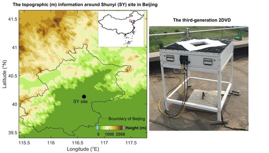
2.1. Data and Instruments

The DSD data ultilized in this research were collected from the field campaigns of the “Storm 973 (dynamic-microphysical-electrical processes in severe thunderstorms and lightning hazards)” Program carried out in Beijing, northern China from 2016 to 2018 [20]. During the observation period, a two-dimensional video disdrometer (2DVD) and a rain gauge (RG) were deployed at the Shunyi national meteorological observation station (SY; 40.13° N, 116.62° E), Beijing, northern China. SY site with an altitude of 30 m AMSL, located at the suburb of the northeast corner of Beijing and adjacent to the Bohai Sea in the east, is a typical semi-humid and semi-arid continental monsoon climatic region. The location of the measurement site is indicated in Figure 1.

The 2-dimensional video distrometer (2DVD) is a particle imaging system based on two orthogonal high-speed line scanning cameras that can record the information of each particle, including the size, fall velocity, and shape. In principle, three-dimensional raindrop shape information of every particle can be recognized through two orthogonal projections [21]. The structure, design, component, and measurement principle of 2DVD can be found in Schönhuber et al. [22]. Many studies have been conducted with this device since it became commercially available [15,23,24,25]. Up to date, the 2DVD has been upgraded to the third generation, which is used in this study. Compared with the previous versions, although the third-generation 2DVD is designed to mitigate the errors caused by raindrop splashing and wind effects [26], some studies have shown that there are still spurious detections of drops, especially for the small raindrops, as well as the splash effect in 2DVD observations [27].

To remove these spurious drops in false terminal fall velocity, a recommended velocity-based filter was applied to the data [21]. Here, the diameter-terminal velocity model described by Brandes et al. [18] was used in the filter. Any raindrop with the velocity that lies outside the ±60% limits of the velocity of Brandes et al. [18] was eliminated. Figure 2 shows the number of raindrops observed by 2DVD on a logarithmic (log₁₀) scale for different diameter size and fall velocity bins during different seasons. In general, the 2DVD measured fall speed of raindrops in each season agreed fairly well with the terminal fall velocity derived using the empirical relation in Brandes et al. [18]. As shown, the peak number of raindrops agrees with the empirical velocity, suggesting a high reliability of the 2DVD measurements. A total of 13,669, 6696, 1301, and 3635 1-min DSD samples are collected using this criterion for summer, fall, winter, and spring rainfall, respectively. In this research, December, January, and February are classified as winter; spring is from March to May; summer is from June to August; and fall includes the months of September, October, and November. As this study mainly focuses on rain, the 2DVD measurements containing snow were removed according to the temperature data measured from automated surface stations at the SY site. In addition, the rain measurements during winter are further confirmed by the particle terminal velocity and diameter relation in [18] (see Figure 2a).

2.2. Methodology

2.2.1. Droplet Size Distribution (DSD)

The DSD [N(D): (mm⁻¹m⁻³)] can be calculated from 2DVD according to the following formula:

$$N(D_i)=\frac{1}{\Delta t\Delta D}{\displaystyle {\sum }_{j=1}^{m_i}\frac{1}{A_j{V}_j}}$$

(1)

where ΔD is the bin size (0.2 mm); Δt is the sampling time (60 s); D_i (mm) is the raindrop diameter at the ith size class; A_j (mm²) is the effective sensing area; V_j (m s⁻¹) denotes the fall velocity for drop j; and m_i is the drop number within the sampling time interval Δt and size bin i.

The widely used gamma distribution [28] was applied to describe the observed DSD,

$$N(D)=N_0{D}^{\mu }{e}^{-\Lambda D}$$

(2)

where D is the raindrop diameter (mm); N₀ (m⁻³ mm^−1-μ) is the number density parameter; Λ (mm⁻¹) is the slope parameter; and μ (dimensionless) is the shape parameter.

The nth-order moment of DSD is defined as follows:

$${\mathrm{M}}_n={\displaystyle {\int }_0^{\infty }{D}^{n}N(D)dD}$$

(3)

Then, we can calculate the mass-weighted mean diameter D_m (mm) and the normalized intercept parameter (N_w) (mm⁻¹m⁻³) [29] as follows:

$$D_m=\frac{M_4}{M_3}=\frac{{\displaystyle \sum _{i=1}^{32}N(D_{\mathrm{i}})D_i^4}\Delta D_i}{{\displaystyle \sum _{i=1}^{32}N(D_{\mathrm{i}})D_i^3}\Delta D_i}$$

(4)

$$N_w=\frac{4^4}{\mathsf{\pi }{\mathsf{\rho }}_w}\left(\frac{{10}^{3}W}{D_m^4}\right)$$

(5)

where ρ_w is the water density (1.0 g cm⁻³).

From the raindrop concentration N(D), integral rainfall parameters such as rain rate R (mm h⁻¹), liquid water content W (g m⁻³), and the total number concentration N_t (m⁻³) can be calculated as follows:

$$R=\frac{6\mathsf{\pi }}{{10}^4}{\displaystyle \sum _{i=1}^L{D}_i^3{V}_{i}N(D_i)}\Delta D_i$$

(6)

$$W=\frac{\mathsf{\pi }}{6\times {10}^3}{\displaystyle \sum _{i=1}^L{D}_i^{3}N(D_i)\Delta D_i}$$

(7)

$$N_t={\displaystyle \sum _{i=1}^{L}N(D_i)}\Delta D_i$$

(8)

where L is the total number of bins; D_i (mm) is the equivalent volume diameter of raindrops for size bin i; and V_i (m s⁻¹) denotes the fall velocity at the diameter D_i. These integral parameters are commonly utilized to describe the microphysical characteristics of precipitation.

2.2.2. Calculated Polarimetric Radar Variables

A high-resolution dual-polarization X-band radar network is being deployed in Beijing for improving the monitoring and prediction of severe weather. Therefore, the theoretical polarimetric variables, including reflectivity at horizontal (Z_h) and vertical polarization (Z_v), differential reflectivity Z_dr, and specific differential phase shift K_dp, were simulated at X-band frequency (9.5 GHz) from the 2DVD data based on the T-matrix scattering approach [30].

$$Z_{h,v}=\frac{4{\lambda }^4}{{\mathsf{\pi }}^4{\left|K_w\right|}^2}{\displaystyle {\int }_{D_{\min }}^{D_{\max }}{\left|f_{hh,vv}(D)\right|}^{2}N(D)dD} [{\mathrm{mm}}^6{\mathrm{m}}^{-3}]$$

(9)

$$Z_{DR}=10{\log }_{10}\left(\frac{Z_h}{Z_v}\right) [\mathrm{dB}]$$

(10)

$$K_{dp}={10}^{-3}\frac{180}{\mathsf{\pi }}\lambda \mathrm{Re}\left\{{\displaystyle {\int }_{D_{\min }}^{D_{\max }}\left[f_h(0,D)-f_v(0,D)\right]N(D)dD}\right\} [° {\mathrm{km}}^{-1}]$$

(11)

where f_hh,vv(D) and f_hh,vv(0, D) are the backscattering and forward-scattering amplitude of a droplet with horizontal and vertical polarization, respectively. The radar wavelength λ is 3.2 cm (X-band). The dielectric factor for water is K_w = 0.93. N(D) is computed from the 2DVD measurements.

2.2.3. Classification of Rain Types

Different precipitation formation mechanisms of convective and stratiform rainfall induce different microphysical characteristics in both rain types [31,32]. In this study, a simple method, similar to the schemes in [33], is used to separate the two rainfall types based on the rainfall rate (R) and the standard deviation (σ_R) over ten consecutive 1-min DSD samples. In particular, it would classify a sample as stratiform rain if R ≥ 0.1 mm h⁻¹ and σ_R ≤ 1.5 mm h⁻¹, and convective rain if R ≥ 5 mm h⁻¹ and σ_R > 1.5 mm h⁻¹. The lower limit of rain rate for seperating stratiform is the same as that in Wen et al. [15] and Tang et al. [14]. Any sample that belongs neither to the stratiform nor convective type is classified as a mixed type and is excluded from the investigation. For the whole datasets obtained from 2DVD, this classification scheme produces 1582 (6.5%) convective samples and 18,741 (76.8%) stratiform samples. Furthermore, there are 10.3% (69.5%), 1.2% (85.5%), 2.7% (86.1%), and 0% (89.6%) convective (stratiform) rainfall samples for summer, fall, spring, and winter, respectively, which indicates that the precipitation in this region is mainly dominated by stratiform rain and the occurrence probability of convective rainfall reaches the highest in summer.

Many studies have investigated the rainfall characteristics under different rain rate classes because the rainfall intensity is closely related to the type of rainfall. For the further analysis of microphysical characteristics of precipitation, the total dataset has been grouped into six categories for DSD parameters (R, D_m, and N_t), akin to Sreekanth et al. [34]. The different bins of R, D_m, and N_t are repeated in

Table 1. Categories of R, D_m, and N_t. Precipitation in this study is divided into six main types based on the rain rate, including moderate drizzle (MD), heavy drizzle/light rain (HD/LR), moderate rain (MD), heavy rain (HR), violent rain (VR), and very violent rain (VVR) [34].

Rain Rate (mm h−1)			Raindrop Diameter (mm)		Raindrop Concentration (m−3)
R Class	Range	Rain Type	Dm Class	Range	Nt Class	Range
R1	0.1~0.5	MD	Dm1	<1	Nt1	10~1000
R2	0.5~2.5	HD/LR	Dm2	1~2	Nt2	1000~2000
R3	2.5~10	MR	Dm3	2~3	Nt3	2000~3000
R4	10~50	HR	Dm4	3~4	Nt4	3000~4000
R5	50~100	VR	Dm5	4~5	Nt5	4000~5000
R6	>100	VVR	Dm6	>5	Nt6	>5000

. For each category of R, D_m, and N_t, the seasonal variability of the average DSD, the frequency of occurrence, the amount of rainfall, and the percentage of contribution to the total rainfall are investigated.

3. Results and Discussions

3.1. Seasonal Variation of Rainfall

Rainfall during 2016–2018 in Beijing presents distinct seasonal variation. Figure 3 shows a unimodal distribution of the three-year mean of annual rainfall with a peak in July and the minimum rainfall amount in winter. The rainfall in fall is more copious than that in spring. A good amount of rainfall, accounting for more than 90% of the three-year total rainfall, is recorded at SY site in summer (June–August) compared with that in the other months. The comparison of monthly rainfall between the two independent instruments (2DVD and rain gauge) at the study site presents an excellent consistency with a correlation coefficient of 0.9991, as shown in the inset graph in Figure 3. For comparison, the coincident rainy time frames of 2DVD and rain gauge were used. During this observation period from 2016 to 2018, a total number of 3551 rain events covering 77,956 min of rain with a total rainfall of 9264.77 mm were observed by the deployed 2DVD. Here, the definition of a rain event was based on the method proposed by Tokay and Bashor [35], i.e., a rain event is defined on the basis of 1 h or a longer rain-free period between two consecutive rainy minutes. The number of rainfall events, total rain duration, seasonal total rainfall, mean rain rate, liquid water content, mass-weighted diameter (D_m), and raindrop concentration (N_t) for each season are listed in

Table 2. The total number of rainfall events, rainfall, and rain duration, as well as the mean values of rain rate, liquid water content, raindrop diameter, and raindrop concentration for each season based on the 2DVD observations.

Season	Winter (December–February)	Spring (March–May)	Summer (June–August)	Fall (September–November)
No. of events	4	15	70	28
Total rain duration (min)	980	4421	16,406	7024
Total rainfall (mm)	13.25	95.08	966.60	145.24
Mean rain rate (mm h−1)	0.86	1.62	4.57	1.52
Mean liquid water content (g m−3)	0.07	0.10	0.24	0.09
Mean Dm (mm)	0.87	1.11	1.32	1.13
Mean Nt (m−3)	410.50	360.76	746.97	400.36

. The values of all rainfall properties reached the highest in summer and the smallest in winter, except for N_t of winter rain. In fall, each value of the rainfall parameter was slightly higher than that in spring except for the mean rain rate and liquid water content. The difference in rainfall parameters of each season implies the unique DSD characteristics of rainfall in each season. Besides, compared with the rain in eastern China [36], the precipitation in Beijing shows lower raindrop concentration for each season. The mean raindrop diameter is slightly larger in summer than that in eastern China, but smaller in the other three seasons.

3.2. DSD of Different Rain Types

Figure 4 shows the composite DSD of six different rain rate bins (R1–R6, Table 1) during four seasons. The width of the DSD in all seasons broadens with the rain intensity. The spectra having large raindrops exceeding 6 mm in high rain rates (R > 10 mm h⁻¹) were observed in spring, summer, and fall, resulting in higher mean values of water content and rain rate and total seasonal rainfall (Table 2) than in winter. Note that there is no rain rate higher than R3 in winter owing to the absence of convective rain during the 2016–2018 period, and the DSDs in winter have the lowest number concentration of raindrops larger than 2.0 mm; moreover, the maximum raindrop diameter is approximately 3.9 mm (Figure 4a–c). The DSD shows seasonal differences in different rain rates, and the seasonal difference is more pronounced in a higher rain rate regime. The raindrop number density N (D) in small drop sizes (D < 1.5 mm) is higher in winter and fall than in spring and summer when R is less than 2.5 mm h⁻¹, while it is lower in larger diameters (D > 2.0 mm) (Figure 4a,b). The differences of DSDs with diameters less than 4 mm are negligible in the R3 category during spring, summer, and fall (Figure 4c). DSDs from R1 to R3 show a single peak with around a diameter of 0.5 mm. N (D) is less than 10³ mm⁻¹m⁻³ and the spectra for all the seasons present a concave-down DSD shape. For R4, R5, and R6, the number densities of small raindrops (D ~ 0.3 mm) for each season is over 10³ mm⁻¹m⁻³ (Figure 4d) and reach 10⁴ mm⁻¹m⁻³ in R5 and R6 (Figure 4e–f). DSDs in R4 show a well-defined peak around diameter of 0.3 mm, followed by a sharp decrease in concentration as the diameter increases to around 0.7 mm in summer and 1.0 mm in srping and fall. Then, the number concentrations decreases exponentially with increasing drop sizes. DSDs in spring and fall are very similar for the R4 categary, and the number density of particles is slightly lower for small diameters (D < 3 mm) than in summer, but higher for larger drops (D > 3 mm) (Figure 4d).

According to the classifications of DSD based on the highest slope (HS) value of DSD between 1.0 and 2.6 mm as described by D’Adderio et al. [37], the DSD of R4 in summer can be classified as the class 3 DSD with an HS value of −0.7, and this type of DSD exhibits a shape with one peak and has an exponential slope from the peak to the largest observed size. The DSD of R5 in spring was similar to that in summer when the drop sizes were smaller than 1.3 mm and showed a smaller concentration for drops between 1.3 and 3.3 mm. In R5, the lowest concentration of raindrops smaller than 3.3 mm occurred in fall, and the three DSDs intersect when the drop size is ~3.3 mm. When raindrop size is larger than 3.3 mm, the number concentration is from high to low for fall, spring, and summer (Figure 4e). In summer, the shape of DSD changes little from R4 to R6, except the increase of number concentration. The R6 category only occurres in summer rain with the highest number concentration of small- to moderate-sized raindrops (D < 4.5 mm), showing a peak (10^4.7 mm⁻¹m⁻³) at the diameter size ~0.3 mm (Figure 4f). These results indicate that the shapes of DSD in MD (R1) and HD/LR (R2) rain categories present similar unimodal distribution in four seasons, and there are minor seasonal distinctions in the small- and large-drop ends. Howerver, the convective rain with a higher rain rate (R > 10 mm h⁻¹) in Beijing shows distinct seasonal variations of DSD.

To explain the seasonal variations of DSD as discussed above, some environmental factors are collected and analyzed. As shown in Figure 5a, the CAPE (convective available potential energy per unit mass) [38] values for the rainy days calculated from the radiosonde data at Beijing site during different seasons are depicted with box-whisker plots. The vertical profiles of mean wind field, temperature, and relative humidity obtained from the radiosonde observations for the rainy days in the four seasons are depicted in Figure 5b–d.

As shown in Figure 5a, the highest value of CAPE, reaching as high as 2275 J kg⁻¹, can be seen during summer, with the mean value at ~709.7 J kg⁻¹, followed by the CAPE in fall and spring, suggesting specific stronger convection activities in summer than in the other two seasons. In addition, the warm and moist air is transported from the Bohai Sea to the continent by the dominant southeasterly winds below the height of less than 850 hPa (Figure 5b), providing favorable conditions for the initiation and development of convective activities in this region, which is prone for the collision and coalescence of raindrops [39]; as a result, the exiguity of large drops in summer was observed (Figure 4). The dominant wind under 850 hPa in fall is also southeasterly. The CAPE value, temperature, and relative humidity are higher in fall than in spring, indicating that the convective activities in fall might be more intense, which helps to produce larger raindrops. Large raindrops will further collect small and/or tiny raindrops through the collision-coalescence process in heavy rain. This might help explain that DSD in fall has more large raindrops, but fewer small- to medium-sized drops in a high rain intensity than in spring (Figure 4e). The CAPE value in winter is negligible because there is no convective rain during winter in Beijing. Cold air from the middle and high latitudes occurred during winter via the prevailing north and northwesterly winds; at the same time, the relative humidity under 850 hPa was relatively higher than that in spring and fall (Figure 5d), thus more small raindrops (D < 1.0 mm) can be retained in low rain intensity. High humidity and low wind speeds might prevent the small raindrops from evaporating during their falling [40]. As shown in Figure 4a,b, the number density of small drops in winter reaches the highest when R is less than 2.5 mm h⁻¹.

3.3. Distributions of D_m and N_w

To further reveal the distinctions of DSD parameters, i.e., D_m and log₁₀N_w, for different rain types, Figure 6 describes the mean, standard deviation of log₁₀N_w and D_m for convective rain (CR) and stratiform rain (SR) in different seasons. For comparative analysis, the mean D_m and log₁₀N_w values obtained in eastern [36] and northwest [41] China are also indicated in Figure 6. In general, the annual averages of D_m and log₁₀N_w are 1.22 mm and 3.84 (mm⁻¹m⁻³ for N_w), respectively. The mean log₁₀N_w in northern China is smaller than that in eastern (3.93) and northwest (3.91) China, while the mean D_m is larger (smaller) than that in estern (eastwest) China. For different rain types, the mean D_m-log₁₀N_w pairs exhibit significant differences in the seasonal pattern in northern China. The CR in summer shows up with the highest log₁₀N_w, but the smallest D_m. The mean D_m (log₁₀N_w) value for CR is approximately 1.84 (3.96), 2.11 (3.65), and 2.42 (3.58) mm in summer, spring, and fall, respectively, which are larger (lower) than that in eastern and northwest China [36] during the same season. On the other hand, the mean values of SR D_m and log₁₀N_w for the four seasons are concentrated in a smaller area (SR: 3.68–3.85 for log₁₀N_w, 0.99–1.28 mm for D_m) than that of CR (CR: 3.58–3.96 for log₁₀N_w, 1.84–2.42 mm for D_m). In addition, the mean D_m-log₁₀N_w pairs for SR appear close to the results in eastern China, and they appear around the leftside of the stratiform line reported by Bringi et al. [42]. However, the mean values of SR D_m and log₁₀N_w in northern and eastern China are both smaller than those of northwest China.

As shown by the errorbars in Figure 6, the difference of the standard deviation (STD) of log₁₀N_w for the same season between CR and SR is not significant. Moreover, for the same rain type, the STD values of log₁₀N_w do not show prominent seasonal variation. In contrast, the STD value of D_m in CR is larger than that in SR for the same season. There is no distinct seasonal variation for the STD of D_m in SR, while the STD value of D_m for CR is 0.70 mm in fall, 0.56 mm in spring, and 0.43 mm in summer (i.e., from large to small).

Previous studies [42,43,44] showed that the different microphysical processes between the maritime and continental convective storms induce considerably different behaviors in the DSD parameters of N_w and D_m. In this study, convective rainfall is not similar to either continental or maritime convective precipitation. The CR in summer and fall slightly tends to the “maritime cluster” and “continental cluster”, respectively.

3.4. Seasonal Variation of R, N_t, and D_m Frequency Distributions and Their Contribution to Rainfall

To further elucidate the microphysical characteristics of rain and their seasonal distinction in Beijing, it is essential to understand rain in terms of its microphysics such as R, D_m, and N_t. These parameters are stratified into six different range bins (Table 1) for all the seasons to further quantify their variation and relative contributions to the total seasonal rainfall. Figure 7 shows the percentage of occurrence frequency (POF) (grey bar) of different categories of rain rate (R1~R6), mean drop diameter (D_m1~D_m2), and raindrop number concentration (N_t1~N_t2) in each season, as well as the percentage of rainfall contribution (PRC) to total rainfall (blue dotted line). The numbers shown on each bar denote the total number of the samples in each range bin.

As shown in Figure 7a–d, the POF of R exhibits an almost similar distribution in the four seasons with a sharp decrease from R2 to R6, even though the occurrence number in each R category varies. Heavy dizzle/light rain (R2) is the major rain type, followed by moderate drizzle (R1) and moderate rain (R3). There were no rain events with a rain rate exceeding R3 (R5) in winter (spring). For the tropical precipitation in India [34], heavy rain with intensity of R4 (10–50 mm h⁻¹) contributes the most to the total rainfall in all seasons, while the largest production of rainfall is from 0.5~5 mm h⁻¹ in Shaanxi, northwest China [41]. The distribution of PRC for R in each rain type varies significantly with the season. During winter and fall, the PRC of R2 reaches the highest, which is 75.1% and 36.6%, respectively. Note that R3 also contributes a comparable total rainfall with 33.4% in fall. The PRC of R in spring shows a bimodal distribution with two approximate peaks (31%) at R4 and R2. During summer, the PRC of R4 is the highest, with near 40%. On the other hand, the contribution from the high rain rates R4 is about 15% in fall. R5 and R6 rain types are disastrous as they can engender an enormous amount of rainfall within a short period [34]. Note that up to 27.9% of total rainfall during summer is from R5 and R6, which easily cause the landslide and flash flood.

Figure 7e–h show a pronounced seasonal variability of POF for D_m, with D_m1 (D_m2) reaching the highest frequency of occurrence during winter and spring (summer and fall). For all the seasons, a steep decrease is exhibited from POF of D_m2 to POF of D_m3. Note that there is no rain exceeding D_m3 in winter. Compared with the other three seasons, summer rain marked the maximum occurrence percentage from the large raindrops (D_m4–D_m6) and had the least POF in D_m1. The distribution of the PRC of D_m is relatively similar in all the seasons, with the D_m2 category registering the highest contribution to the total rainfall. The POF of large raindrops (D_m4–D_m6) is the highest in summer, followed by spring and fall; however, these large raindrops contribute less than 6% of the total rainfall. The large drops with D_m > D_m4 were mainly observed during the intense convective rainstorms from April to September. A combination of many factors, such as the more effective collision-coalescence of raindrops, relatively wet atmospheric background in the warm season, and the dynamic and thermodynamic conditions in the clouds, may lead to the occurrence of large raindrops up to D_m5–D_m6 in warm-rain clouds.

Figure 7i–l demonstrate the seasonal distribution of the POF and PRC of N_t. For the four seasons, the N_t1 category is dominated in the frequency of occurrence of N_t bins, followed by a steep decrease in the subsequent bins. A steady decrease in the POF and PRC from N_t2 to N_t5 and an apparent increase in the subsequent N_t6 are observed in all the seasons except for winter, when there is no N_t6 category. The distribution of PRC for different N_t bins in spring and fall is quite similar. During summer, the PRC of N_t1 is the lowest (34.7%), which exhibits high values in the other three seasons with a mean value of 77.8%. Although the most frequent N_t1 registers the most relative rainfall contribution for the other three seasons, N_t6 contributes the most total rainfall in summer. Approximately 36.6% of total rainfall from N_t6 (>5000 m⁻³) drops range, indicating the high concentration of raindrops in summer. Moreover, the increased PRC of N_t6 during summer is well supported by the increased POF of D_m2.

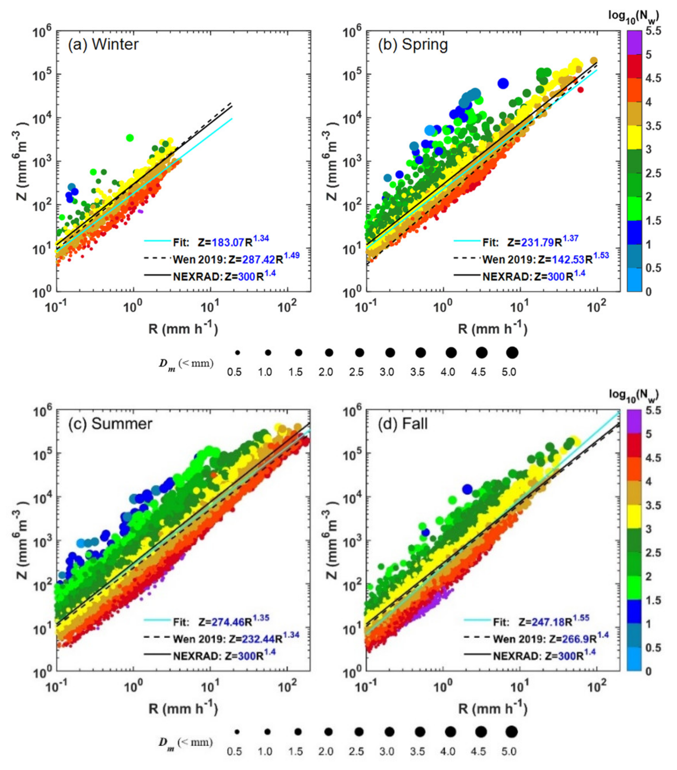
3.5. Derived Relations

3.5.1. μ–Λ Relations

Previous studies [14,25,43,45,46] have shown that the μ–Λ relations vary in different regions, depending on the local raindrop spectrum characteristics. The μ–Λ relation provides an insight into the DSD characteristics and simplifies the polarization variables in the retrieval of DSD from dual-polarization radar. Zhang et al. [47] used an empirical relation: Λ = 0.0365μ² + 0.735μ + 1.935, derived under the condition of R > 5 mm h⁻¹ and N_t > 1000 m⁻³, to retrieve DSD from polarimetric radar measurements. He suggested that the μ–Λ relation is more suitable for the range of Λ from 0 to 20 because large Λ values contain a larger measurement error rather than the microphysical process of precipitation. In this study, therefore, the same threshold criterion proposed by Zhang et al. [43] is applied to minimize the sampling errors. It is noted that there are no samples in winter that can go through the data filter owing to the absence of convective rain. Thus, the µ–Λ relations for the other three seasons and the total dataset are analyzed and presented in Figure 8. In addition, the µ–Λ relations derived from other measurements in different regions (e.g., Florida [47], Nanjing [43], Zhangbei [14], and Zhuhai [46]) are also depicted by the dashed lines in Figure 8. Therein, the data observed in Florida were collected from 2DVD and the other data sets were observed by Parsivel.

It is evident from Figure 8 that the μ–Λ relations in our study vary little among seasons and they are close to Florida relation [47]. Such similarities could be related to the same type of instrument measurements as well as the applied filter threshold. Relations in Chen et al. [43], Tang et al. [14], and Zhang et al. [46] are similar to each other, and for a given Λ, these relations have higher µ than our relation. Previous studies [48,49,50] have shown that higher µ values may be attributed in part to the underestimation of small drops by the Parsivel. 2DVD was used in this study and Florida [47], so the differences in μ–Λ relations in different regions obtained by the same instrument are related to the microphysical processes of rainfall in different climatic regimes. As shown in Figure 8, the difference between the two curves obtained in Beijing and Florida gradually becomes pronounced when μ > 10. For a given μ, the value of Λ is smaller in our relationship, which implies that the D_m might be larger than that in Florida because D_m is inversely proportional to Λ when μ is known.

3.5.2. Z–R Relations

The power–law relationship Z = AR ^b derived using disdrometer measurements has been widely used for radar quantitative precipitation estimation (QPE). Owing to the significant variability of DSD, the equations of Z = AR ^b are also changeable [4,51,52,53]. The different dynamics and microphysical processes are the main reasons for the distinction in Z–R relationships between mid-latitude and tropical precipitation [4,53]. Figure 9 shows the scatter distribution of Z–R pairs color-coded by log₁₀N_w, and the size of the circles represents the magnitude of D_m. The power–law formulations of Z–R relationships in each season are also fitted using the least-squares method and given by the cyan lines in Figure 9. For comparison, the standard WSR-88D relation (i.e., Z = 300R^1.4, [54]), which is adopted by the operational weather radar systems in China (the solid black lines), and the eastern China Z–R relationships in each season are also plotted in Figure 9.

During winter, the rainfall is entirely composed of stratiform and all the 1-min rain rates are less than 10 mm h⁻¹ (Figure 9a), resulting in the lowest value of A and b (Z = 183.07R^1.34), compared with the other three seasons. Moreover, the fitting curve locates below the Z–R relationship of eastern China and the standard Z–R relation (Z = 300R^1.4) (Figure 9a). In spring, the Z–R relationship (Z = 231.79R^1.37) in this study lies between the other two Z–R relationships except for the R exceeding 25 mm h⁻¹ (Figure 9b). The Z–R relation in summer (Z = 274.46R^1.35) is nearest to the standard relationship (Figure 9c), suggesting the relationship of the operational WSR-88D could be properly employed for QPE in Beijing to estimate the summer rain. During fall, the exponent b of the Z–R relation is the highest (Z = 247.18R^1.55). For a given Z, this relation leads to a lower (higher) R than the Z–R relation of eastern China and the standard relationship when R is higher (less) than 10 mm h⁻¹ (Figure 9d).

From the above analysis, it is concluded that Z–R relaionships not only vary with seasons, but also change with geographical location owing to the variability of DSD in different seasons and regions. The two coefficients A and b are dependent on the DSD characteristics. Therein, the coefficient A is proportional to D_m (Steiner et al., 2014). As shown in Table 2, the mean values of D_m (coefficient A) are 1.32 mm (274.46) in summer, 1.13 mm (247.18) in fall, 1.11 mm (231.79) in spring, and 0.87 mm (193.07) in winter. The exponent b shows slight differences among seasons and ranges from 1.34 to 1.55 (within range 1.0 ≤ b ≤ 1.63, see Figure 1 in Steiner et al. [55]), indicating that the variability of DSDs in each season is controlled by a coordinated mix of variations in number concentration and drop size [55], which is different from the tropical oceanic rain characterized by concentration-controlled DSD variability [23]. In addition, Figure 9 shows that the same D_m can result in different reflectivities and/or rain rates depending on the number concentration. A majority of the DSDs with low log₁₀N_w (<1.5) and large D_m (>4.0 mm) exist above the area for Z > 20 dBZ, while the higher log₁₀N_w values ranging from >5 appear only in the lower mode of the Z (R) distributions, which indicates that the radar measurements are insensitive to small raindrops when large raindrops are present. In general, as shown in Figure 9, Z–R relationships change with seasons, hence it is worth considering such variability in improving radar-based QPE.

3.5.3. Axis Ratio versus Drop Diameter

The raindrop axis ratio (drop shape ratio—DSR) relations play an essential role in the derivation of polarimetric radar rainfall algorithms based on polarimetric radar parameters, i.e., Z_DR and K_DP [56,57,58]. In this section, the mean axis-ratio relation obtained in the natural atmospheric environment and several polarimetric rainfall algorithms developed using 2DVD measurements are studied. For comparison, four raindrop shape assumptions (i.e., PB70, BC87, BR02, and TH07) obtained in various conditions are also used to derive the algorithms.

Figure 10 shows the frequency distribution (in a logarithmic scale) of every drop axis ratio bin of 0.02 (dimensionless) and equivolumetric diameter interval of 0.2 mm for the four seasons. There are still significant particles with a diameter less than 1.5 mm having an axis ratio less than 0.5, and some small drops have an axis ratio exceeding 1.5. This may be related to the instrumental uncertainty [59,60]. As reported in Larsen et al. [27], these outliers cannot be completely excluded by merely applying a velocity-based filter to the data. Therefore, akin to the procedures of Chang et al. [59], the axis ratios of raindrops with a diameter less than 1 mm were artificially set to nearly 1. Moreover, the fitting relation of mean axis ratio versus diameter was constructed within 3.0 mm for winter and within 4.5 mm diameter for the other three seasons to have enough raindrops.

As shown in Figure 10a–d, the frequency distribution characteristics of axis ratio versus diameter for all seasons are relatively consistent, although the fourth-order polynomial fitting formulas change with the season. The fourth-order polynomial mean axis-ratio relations for the whole dataset and the different seasons are given in Equations (12)–(16), respectively:

b/a = −3.139 × 10⁻⁴D⁴ + 5.528 × 10⁻³D³ − 3.325 × 10⁻²D² + 2.869 × 10⁻²D + 0.9871 (Total)

(12)

b/a = −6.363 × 10⁻⁴D⁴ + 1.060 × 10⁻²D³ − 6.141 × 10⁻²D² + 7.621 × 10⁻²D + 0.9802 (Winter)

(13)

b/a = −1.575 × 10⁻⁴D⁴ + 3.445 × 10⁻³D³ − 2.781 × 10⁻²D² + 3.873 × 10⁻²D + 0.9869 (Spring)

(14)

b/a = −1.346 × 10⁻⁴D⁴ + 3.221 × 10⁻³D³ − 2.421 × 10⁻²D² + 1.699 × 10⁻²D + 0.9882 (Summer)

(15)

b/a = −1.182 × 10⁻⁴D⁴ + 2.180 × 10⁻³D³ − 1.690 × 10⁻²D² − 4.992 × 10⁻³D + 1.0016 (Fall)

(16)

where a and b are the major and minor axises of a particle, respectively, and D (mm) is the equivalent raindrop diameter.

In general, the mean axis ratio relation fitted from the measurements in Beijing is more spherical than the other three empirical relations (the dashed curves in Figure 10e) and shows seasonal varibility. Compared with summer and fall, the mean axis ratio (closer to 1) for raindrops between 0.4 and 1.3 mm in diameter in winter and spring is more spherical. The spring axis-ratio relation for 1.5 ≤ D ≤ 6.5 mm is higher than that of the other three seasons (Figure 10e). The summer DSR is close to that derived from the whole dataset, while the mean axis ratio is lower in fall and winter than in summer, especially for diameter larger than 3 mm, and reaches the maximum in spring. The horizaontal wind may be a factor that affects the raindrop shape. Chang et al. [59] and Wen et al. [61] both found that the DSR is more spherical than that of Brandes et al. [18], and they attributed this spherical DSR to the higher horizaontal wind. However, to isolate the specific causes, further observational experiments and aerodynamics model study are needed.

The polarimetric variables are sensitive to the raindrop shapes. Therefore, the impact of different axis-ratio relations on the polarimetric radar parameters is discussed. Here, the new fitted axis-ratio Equation (12) for the entire data set was considered in the following analysis. Firstly, the dual-polarimetric variables at the X-band of 3.2 cm wavelength were calculated using Equations (9)–(11) based on different axis-ratio relations using the T-matrix method. The temperature is assumed to be 20 °C. The mean and standard deviation of the raindrop canting angle are set to 0° and 7°, respectively [62]. Secondly, the polarimetric rainfall algorithms incuding R (K_dp), R (Z_h, Z_dr), and R (Z_dr, K_dp) were deduced and compared with R (Z_h).

Referring to Figure 11, the relationship between Z_DR and Z_H (Figure 11a) is more exponential other than the linear relationship between Z_DR and Z_H reported by Park et al. [63]; moreover, there is a distinct exponential relationship between K_dp and Z_H (Figure 11b). Z_DR and K_dp increase with Z_H. Note that the polarimetric variables based on the shape of raindrops in Beijing increase less rapidly than that from other raindrop shape models when Z_H is larger than 40 dBZ (for Z_DR) and 60 dBZ (for K_dp) (Figure 11c,d). This is probably related to the larger axis-ratio of large raindrops observed in Beijing, as shown in Figure 10e. The raindrop keeps a more spherical shape in the process of increasing, which makes Z_H increase rapidly, but contributes less to Z_DR and K_dp.

Table 3. Information for the fitted Z_DR-Z_H and K_dp-Z_H relationships at the X-band radar (3.2 cm) and 20 ℃ derived under different axis-ratio relations.

Raindrop Shape Models	ZDR = aZH b		Kdp = cZH d
	a	b	c	d
PB70	0.0051	1.5523	6.85 × 10−8	4.3282
BC87	0.0011	1.9307	1.51 × 10−8	4.6660
BR02	0.0004	2.1974	4.67 × 10−9	4.9473
TH07	0.0005	2.1290	6.71 × 10−9	4.8664
New	0.0012	1.7724	3.16 × 10−8	4.3216

lists the coefficients of these fitted exponential relationships between Z_DR, K_dp, and Z_H. For a given Z, the other relations have larger Z_DR and K_dp values than those from our fitting relations.

To further investigate the impact of the raindrop shape on the polarimetric rainfall estimations, the rain rate R_e estimated from various QPE algorithms based on polarimetric variables (

Table 4. Comparison results (CC, RMSE and NE) of rain rate derived from 2DVD (R) and estimated from QPE algorithms (R_e) based on different raindrop shape models.

R (Zh) = αZhβ
	α	β	CC	RMSE	NE		Raindrop Shape Models
1	0.0234	0.6567	0.82	5.92	0.45		PB70
2	0.0238	0.6559	0.81	6.12	0.46		BC87
3	0.0237	0.6572	0.81	6.06	0.45		BR02
4	0.0261	0.6427	0.80	5.82	0.47		TH07
5	0.0238	0.6567	0.82	5.77	0.45		New
R (Kdp) = αKdpβ
	α	β	CC	RMSE	NE		Raindrop Shape Models
1	11.1818	0.8480	0.98	2.14	0.17		PB70
2	13.3291	0.7837	0.98	2.80	0.23		BC87
3	14.0583	0.7345	0.97	3.40	0.28		BR02
4	13.5500	0.7368	0.97	3.41	0.27		TH07
5	21.9257	0.8419	0.98	1.85	0.18		New
R (Zh,Zdr) = αZhβ100.1γZdr
	α	β	γ		CC	RMSE	NE	Raindrop Shape Models
1	0.0125	0.9488	−5.4400		0.98	2.70	0.17	PB70
2	0.0112	0.9146	−4.8392		0.98	3.25	0.21	BC87
3	0.0108	0.9025	−4.7226		0.98	3.40	0.22	BR02
4	0.0112	0.9123	−4.8495		0.98	3.23	0.21	TH07
5	0.0114	0.9130	−7.3969		0.98	3.29	0.21	New
R (Kdp,Zdr) = αKdpβ100.1γZdr
	α	β	γ		CC	RMSE	NE	Raindrop Shape Models
1	19.6049	0.9397	−1.5455		0.98	2.70	0.17	PB70
2	25.6583	0.8933	−1.9110		0.97	3.48	0.22	BC87
3	28.2863	0.8495	−2.1187		0.96	4.13	0.26	BR02
4	26.7898	0.8473	−2.0690		0.96	4.13	0.26	TH07
5	45.6066	0.9590	−3.0565		0.98	2.16	0.14	New

) was compared with R derived directly from 2DVD results—Equation (6). The evaluation metrics to quantify the performance of each QPE algorithm include the correlation coefficient (CC), root-mean-square error (RMSE), and the normalized absolute error (NE). They are calculated according to Equations (17)–(19):

$$CC=\frac{{{\displaystyle \sum }}_{i=1}^n\left(R_i-\overline{R}\right)\left(R_{e,i}-\overline{R_e}\right)}{{\left[{{\displaystyle \sum }}_{i=1}^n\left(R_i-\overline{R}\right)\right]}^{1/2}{\left[{{\displaystyle \sum }}_{i=1}^n\left(R_{e,i}-\overline{R_e}\right)\right]}^{1/2}}$$

(17)

$$RMSE={\left(\frac{1}{n}{\displaystyle \sum }_{i=1}^n{R}_i-R_{e,i}\right)}^{0.5}$$

(18)

$$NE=\frac{\frac{1}{n}{{\displaystyle \sum }}_{i=1}^n\left|R_i-R_{e,i}\right|}{\overline{R}}$$

(19)

where R and R_e are the observed rain rate from 2DVD and the estimated rainfall rates with QPE algorithms (Table 4), respectively. The n is the number of sample pairs and “¯” represents the sample average. Figure 12 illustrates the scatterplot of R versus R_e estimated from polarimetric rainfall relations derived using the new axis-ratio model in this study. The dispersion of the scatters suggests the large effect of DSD variability on rainfall estimations. As shown in Figure 12, it is evident that three QPE algorithms based on Z_dr and K_dp perform much better than R (Z_h), which performs the worst with broadly distributed scatters and overestimations (Figure 12a). Notably, R (K_dp, Z_dr) and R (K_dp) present similar performance under the “ideal” conditions with the high CC of 0.98 for both estimators and small NE values of 0.15 mm h⁻¹ and 0.18 mm h⁻¹, as well as low RMSE values of 1.87 mm h⁻¹ and 1.85 mm h⁻¹ for R (K_dp, Z_dr) and R (K_dp), respectively (Figure 12d). Compared with the polarimetric rainfall relations, the highest RMSE (5.76 mm h⁻¹) and NE (0.45 mm h⁻¹), but the lowest CC (0.82) are found in the use of the R (Z_h), indicating that the Q2PE estimators based on polarization parameters mitigate the effect of DSD variability on the rainfall estimation. Similar results can be found in the polarimetric rainfall algorithms based on other axis-ratio relations (Table 4) with the CC of 0.96~0.99. R (Z_h) estimators based on all axis-ratio relations have lower CC (0.80~0.82), along with higher NE (0.45~0.47 mm h⁻¹) and RMSE (5.77~6.12 mm h⁻¹). Note that the R (Z_dr, K_dp) based on the new axis-ratio relationship shown the best performance; however, the performance of the polarimetric rainfall relations in practical conditions also depends on the different error structures of dual-polarization radar measurements. Therefore, more detailed analyses should be carried out on quantifying the impact of different axis-ratio relations on polarimetric rainfall estimates using multiple precipitation cases in the future.

4. Conclusions

The seasonal variations of rainfall microphysics in Beijing, northern China are investigated using observations from a 2DVD disdrometer during 2016–2018. For the first time, the seasonal differences in DSD and the raindrop shapes in northern China are quantified. In addition, the polarimetric radar rainfall algorithms were derived based on various raindrop axis ratio relationships; moreover, the impact of different raindrop shape models on the polarimetric parameters was discussed. The main conclusions are summarized as follows:

(1)

There exist significant seasonal differences in DSD and rainfall in Beijing. The least rainy season is winter with a large number of small raindrops and the maximum raindrop is approximately 4 mm in diameter. The total raindrop concentration N_t peaked in summer and the mean annual rainfall peaked in July. Small- to medium-sized raindrops (D < 3.5 mm) are more prevalent during July and August, whereas larger raindrops (D > 4 mm) are more abundant in June. The shape of averaged DSD in spring and fall is similar for a diameter of less than 2.5 mm, but the number density of raindrops exceeding 2.5 mm is slightly more in spring.

(2)

The DSD in different rain rates exhibits significant seasonal variation. The width of DSD broadens with the increasing rain rate. DSD for each season presents a unimodal (bimodal) model when R is less (more) than 10 mm h⁻¹. The mean D_m and log₁₀N_w of stratiform rainfall for all seasons are near the “stratiform line” given by [32]. The convective rain in summer is close to the “maritime-like” cluster, whereas there was no distinguishable “maritime-like” or “continental-like” convective precipitation in spring and fall. The causative mechanisms responsible for the seasonal variations of DSD are investigated. Significant differences in temperature, relative humidity, wind velocity, and CAPE value may account for the distinctions in the DSD during different seasons.

(3)

The light rain (R2 category: 0.2–2.5 mm h⁻¹) has the highest occurrence frequency throughout the year, followed by R1 (0.1–0.5 mm h⁻¹). The high occurrence of R5 and R6 manifests the rain intensity of summer precipitation in Beijing. The rainfall is dominated by the small raindrops (D_m2: 1~2 mm) for all seasons in Beijing. Among N_t bins, the lowest raindrop concentration category N_t1 registers the maximum occurrence and rainfall percentages for all seasons, except for the summer, where the rainfall is contributed primarily from the N_t6 (>5000 m⁻³).

(4)

There were no significant seasonal differences in the shape–slope relations. For a given slope value, the μ value in this study is less than that derived from other regions of China. The Z–R relationship changes with the seasons owing to the seasonal variations of DSD. Therein, the Z–R relationship in summer is closest to the NEXRAD Z–R relationship.

(5)

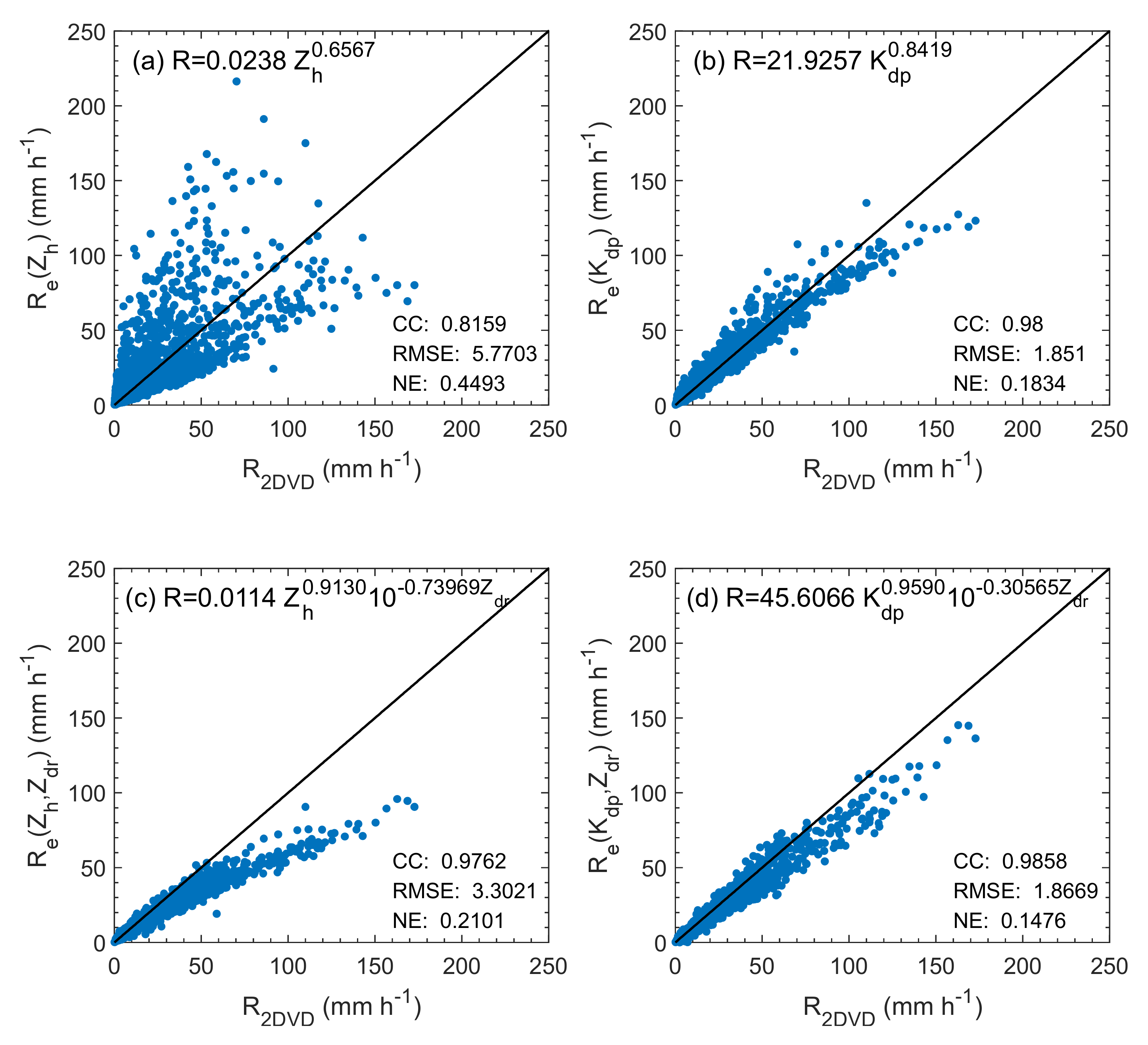
The shape of raindrops in Beijing was more spherical than those obtained with other empirical relations from PB70, BC87, BR02, and TH07. The polarimetric rainfall relations at X-band frequency derived based on various raindrop shape models showed that R (K_dp, Z_dr) using the new axis-ratio relation performs the best under “ideal” conditions.

In general, this study gives an insight into the seasonal variations of DSD and the shape of raindrops in Beijing, which could serve as a reference for optimizing the polarimetric rainfall algorithms for the Beijing urban radar network. However, it is still necessary to further investigate the characteristics of DSD to obtain more information about the microphysical characteristics of precipitation in Beijing. Moreover, the polarimetric radar rainfall relations derived using different raindrop shape models should be verified and evaluated through cross-comparison with rain gauge observations in future.

References

1. Jankov, I.; Bao, J.-W.; Neiman, P.J.; Schultz, P.J.; Yuan, H.; White, A.B. Evaluation and comparison of microphysical algorithms in ARW-WRF model simulations of atmospheric river events affecting the California coast. J. Hydrometeorol. 2009, 10, 847–870. [Google Scholar] [CrossRef]
2. Orr, A.; Listowski, C.; Couttet, M.; Collier, E.; Immerzeel, W.; Deb, P.; Bannister, D. Sensitivity of simulated summer monsoonal precipitation in Langtang Valley, Himalaya, to cloud microphysics schemes in WRF. J. Geophys. Res. Atmos. 2017, 122, 6298–6318. [Google Scholar] [CrossRef] [Green Version]
3. Morrison, H.; van Lier-Walqui, M.; Fridlind, A.M.; Grabowski, W.W.; Harrington, J.Y.; Hoose, C.; Korolev, A.; Kumjian, M.R.; Milbrandt, J.A.; Pawlowska, H.; et al. Confronting the challenge of modeling cloud and precipitation microphysics. J. Adv. Modeling Earth Syst. 2020, 12. [Google Scholar] [CrossRef] [PubMed]
4. Rosenfeld, D.; Ulbrich, C.W. Cloud microphysical properties, processes, and rainfall estimation opportunities. Meteorol. Monogr. 2003, 52, 237–258. [Google Scholar] [CrossRef]
5. Bringi, V.N.; Chandrasekar, V. Polarimetric Doppler Weather Radar: Principles and Applications; Cambridge University Press: Cambridge, UK, 2001. [Google Scholar] [CrossRef]
6. Chen, H.; Chandrasekar, V.; Bechini, R. An Improved Dual-Polarization Radar Rainfall Algorithm (DROPS2.0): Application in NASA IFloodS Field Campaign. J. Hydrometeorol. 2017, 18, 917–937. [Google Scholar] [CrossRef]
7. Cifelli, R.; Chandrasekar, V.; Lim, S.; Kennedy, P.C.; Wang, Y.; Rutledge, S.A. A new dual-polarization radar rainfall algorithm: Application in Colorado precipitation events. J. Atmos. Ocean. Technol. 2011, 28, 352–364. [Google Scholar] [CrossRef] [Green Version]
8. Cohen, C.; McCaul, E.W., Jr. The sensitivity of simulated convective storms to variations in prescribed single-moment microphysics parameters that describe particle distributions, sizes, and numbers. Mon. Weather Rev. 2006, 134, 2547–2565. [Google Scholar] [CrossRef] [Green Version]
9. Fadnavis, S.; Deshpande, M.; Ghude, S.D.; Raj, P.E. Simulation of severe thunder storm event: A case study over Pune, India. Nat. Hazards 2014, 72, 927–943. [Google Scholar] [CrossRef]
10. Gilmore, M.S.; Straka, J.M.; Rasmussen, E.N. Precipitation uncertainty due to variations in precipitation particle parameters within a simple microphysics scheme. Mon. Weather Rev. 2004, 132, 2610–2627. [Google Scholar] [CrossRef]
11. McFarquhar, G.M.; Hsieh, T.-L.; Freer, M.; Mascio, J.; Jewett, B.F. The characterization of ice hydrometeor gamma size distributions as volumes inN0-λ-μphase space: Implications for microphysical process modeling. J. Atmos. Sci. 2015, 72, 892. [Google Scholar] [CrossRef]
12. Ji, L.; Chen, H.; Li, L.; Chen, B.; Xiao, X.; Chen, M.; Zhang, G. Raindrop size distributions and rain characteristics observed by a PARSIVEL disdrometer in Beijing, Northern China. Remote Sens. 2019, 11, 1479. [Google Scholar] [CrossRef] [Green Version]
13. Ma, Y.; Ni, G.; Chandrasekar, V.; Tian, F.; Chen, H. Statistical characteristics of raindrop size distribution during rainy seasons in Beijing urban area and implications for radar rainfall estimation. Hydrol. Earth Syst. Sci. Discuss. 2019, 2019, 1–34. [Google Scholar] [CrossRef] [Green Version]
14. Tang, Q.; Xiao, H.; Guo, C.W.; Feng, L. Characteristics of the raindrop size distributions and their retrieved polarimetric radar parameters in northern and southern China. Atmos. Res. 2014, 135, 59–75. [Google Scholar] [CrossRef]
15. Wen, G.; Xiao, H.; Yang, H.L.; Bi, Y.H.; Xu, W.J. Characteristics of summer and winter precipitation over northern China. Atmos. Res. 2017, 197, 390–406. [Google Scholar] [CrossRef]
16. Pruppacher, H.R.; Beard, K.V. A wind tunnel investigation of the internal circulation and shape of water drops falling at terminal velocity in air. Q. J. Royal Meteorol. Soc. 1970, 96, 247–256. [Google Scholar] [CrossRef]
17. Beard, K.V.; Chuang, C. A New model for the equilibrium shape of raindrops. J. Atmos. Sci. 1987, 44, 1509–1524. [Google Scholar] [CrossRef]
18. Brandes, E.A.; Zhang, G.F.; Vivekanandan, J. Experiments in rainfall estimation with a polarimetric radar in a subtropical environment. J. Appl. Meteorol. 2002, 41, 674–685. [Google Scholar] [CrossRef] [Green Version]
19. Thurai, M.; Huang, G.J.; Bringi, V.N.; Randeu, W.L.; Schönhuber, M. Drop shapes, model comparisons, and calculations of polarimetric radar parameters in rain. J. Atmos. Ocean. Technol. 2007, 24, 1019–1032. [Google Scholar] [CrossRef]
20. Qie, X.; Yuan, S.; Chen, Z.; Wang, D.; Liu, D.; Sun, M.; Sun, Z.; Srivastava, A.; Zhang, H.; Lu, J.; et al. Understanding the dynamical-microphysical-electrical processes associated with severe thunderstorms over the Beijing metropolitan region. Sci. China Earth Sci. 2020. [Google Scholar] [CrossRef]
21. Kruger, A.; Krajewski, W.F. Two-dimensional video disdrometer: A description. J. Atmos. Ocean. Technol. 2002, 19, 602–617. [Google Scholar] [CrossRef]
22. Schönhuber, M.; Lammer, G.; Randeu, W.L. The 2D-video-distrometer. In Precipitation: Advances in Measurement, Estimation and Prediction; Michaelides, S., Ed.; Springer: Berlin/Heidelberg, Germany, 2008; pp. 3–31. [Google Scholar] [CrossRef]
23. Thompson, E.J.; Rutledge, S.A.; Dolan, B.; Thurai, M. Drop size distributions and radar observations of convective and stratiform rain over the equatorial Indian and West Pacific Oceans. J. Atmos. Sci. 2015, 72, 4091–4125. [Google Scholar] [CrossRef]
24. Thurai, M.; Gatlin, P.N.; Bringi, V.N. Separating stratiform and convective rain types based on the drop size distribution characteristics using 2D video disdrometer data. Atmos. Res. 2016, 169, 416–423. [Google Scholar] [CrossRef]
25. Wen, L.; Zhao, K.; Zhang, G.F.; Xue, M.; Zhou, B.W.; Liu, S.; Chen, X.C. Statistical characteristics of raindrop size distributions observed in East China during the Asian summer monsoon season using 2-D video disdrometer and Micro Rain Radar data. J. Geophys. Res.Atmos. 2016, 121, 2265–2282. [Google Scholar] [CrossRef] [Green Version]
26. Schönhuber, M.; Lammer, G.; Randeu, W.L. One decade of imaging precipitation measurement by 2D-video-distrometer. Adv. in Geosci. 2007, 10, 85–90. [Google Scholar] [CrossRef] [Green Version]
27. Larsen, M.L.; Schoenhuber, M. Identification and characterization of an anomaly in two-dimensional video disdrometer data. Atmosphere 2018, 9, 315. [Google Scholar] [CrossRef] [Green Version]
28. Ulbrich, C.W. Natural variations in the analytical form of the raindrop size distribution. J. Clim. Appl. Meteorol. 1983, 22, 1764–1775. [Google Scholar] [CrossRef] [Green Version]
29. Testud, J.; Oury, S.; Black, R.A.; Amayenc, P.; Dou, X.K. The concept of “normalized” distribution to describe raindrop spectra: A tool for cloud physics and cloud remote sensing. J. Appl. Meteorol. 2001, 40, 1118–1140. [Google Scholar] [CrossRef]
30. Waterman, P.C. Matrix formulation of electromagnetic scattering. Proc. IEEE 1965, 53, 805–812. [Google Scholar] [CrossRef]
31. Fujiwara, M. Raindrop-size distribution from individual storms. J. Atmos. Sci. 1965, 22, 585–591. [Google Scholar] [CrossRef] [Green Version]
32. Stout, G.E.; Mueller, E.A. Survey of relationships between rainfall rate and radar reflectivity in the measurement of precipitation. J. Appl. Meteorol. 1968, 7, 465–474. [Google Scholar] [CrossRef] [Green Version]
33. Marzano, F.S.; Cimini, D.; Montopoli, M. Investigating precipitation microphysics using ground-based microwave remote sensors and disdrometer data. Atmos. Res. 2010, 97, 583–600. [Google Scholar] [CrossRef]
34. Sreekanth, T.S.; Varikoden, H.; Mohan-Kumar, G.; Resmi, E.A. Microphysical features of rain and rain events during different seasons over a tropical mountain location using an optical disdrometer. Sci. Rep. 2019, 9, 19083. [Google Scholar] [CrossRef] [Green Version]
35. Tokay, A.; Bashor, P.G. An Experimental study of small-scale variability of raindrop size distribution. J. Appl. Meteorol. Climatol. 2010, 49, 2348–2365. [Google Scholar] [CrossRef]
36. Wen, L.; Zhao, K.; Wang, M.; Zhang, G. Seasonal variations of observed raindrop size distribution in East China. Adv. Atmos. Sci. 2019, 36, 346–362. [Google Scholar] [CrossRef]
37. D’Adderio, L.P.; Porcu, F.; Tokay, A. Identification and analysis of collisional breakup in natural rain. J. Atmos. Sci. 2015, 72, 3404–3416. [Google Scholar] [CrossRef]
38. Moncrieff, M.W.; Miller, M.J. The dynamics and simulation of tropical cumulonimbus and squall lines. Q. J. R. Meteorol. Soc. 1976, 102, 373–394. [Google Scholar] [CrossRef]
39. Andreae, M.O.; Rosenfeld, D.; Artaxo, P.; Costa, A.A.; Frank, G.P.; Longo, K.M.; Silva-Dias, M.A.F. Smoking rain clouds over the Amazon. Science 2004, 303, 1337. [Google Scholar] [CrossRef] [Green Version]
40. McVicar, T.R.; Roderick, M.L.; Donohue, R.J.; Li, L.T.; Van Niel, T.G.; Thomas, A.; Grieser, J.; Jhajharia, D.; Himri, Y.; Mahowald, N.M.; et al. Global review and synthesis of trends in observed terrestrial near-surface wind speeds: Implications for evaporation. J. Hydrol. 2012, 416–417, 182–205. [Google Scholar] [CrossRef]
41. Xie, Z.; Yang, H.; Lv, H.; Hu, Q. Seasonal characteristics of disdrometer-observed raindrop size distributions and their applications on radar calibration and erosion mechanism in a semi-arid area of China. Remote Sens. 2020, 12, 262. [Google Scholar] [CrossRef] [Green Version]
42. Bringi, V.N.; Chandrasekar, V.; Hubbert, J.; Gorgucci, E.; Randeu, W.L.; Schoenhuber, M. Raindrop size distribution in different climatic regimes from disdrometer and dual-polarized radar analysis. J. Atmos. Sci. 2003, 60, 354–365. [Google Scholar] [CrossRef]
43. Chen, B.J.; Yang, J.; Pu, J.P. Statistical characteristics of raindrop size distribution in the Meiyu season observed in Eastern China. J. Meteorol. Soc. Jpn. 2013, 91, 215–227. [Google Scholar] [CrossRef] [Green Version]
44. Ulbrich, C.W.; Atlas, D. Microphysics of raindrop size spectra: Tropical continental and maritime storms. J. Appl. Meteorol. Climatol. 2007, 46, 1777–1791. [Google Scholar] [CrossRef]
45. Cao, Q.; Zhang, G.; Brandes, E.; Schuur, T.; Ryzhkov, A.; Ikeda, K. Analysis of video disdrometer and polarimetric radar data to characterize rain microphysics in Oklahoma. J. Appl. Meteorol. Climatol. 2008, 47, 2238–2255. [Google Scholar] [CrossRef] [Green Version]
46. Zhang, A.; Hu, J.; Chen, S.; Hu, D.; Liang, Z.; Huang, C.; Xiao, L.; Min, C.; Li, H. Statistical characteristics of raindrop size distribution in the monsoon season observed in Southern China. Remote Sens. 2019, 11, 432. [Google Scholar] [CrossRef] [Green Version]
47. Zhang, G.; Vivekanandan, J.; Brandes, E.A.; Meneghini, R.; Kozu, T. The shape–slope relation in observed gamma raindrop size distributions: Statistical error or useful information? J. Atmos. Ocean. Technol. 2003, 20, 1106–1119. [Google Scholar] [CrossRef] [Green Version]
48. Thurai, M.; Petersen, W.A.; Tokay, A.; Schultz, C.; Gatlin, P. Drop size distribution comparisons between Parsivel and 2-D video disdrometers. Adv. Geosci. 2011, 30, 3–9. [Google Scholar] [CrossRef] [Green Version]
49. Tokay, A.; Petersen, W.A.; Gatlin, P.; Wingo, M. Comparison of raindrop size distribution measurements by collocated disdrometers. J. Atmos. Ocean. Technol. 2013, 30, 1672–1690. [Google Scholar] [CrossRef]
50. Wen, L.; Zhao, K.; Zhang, G.F.; Liu, S.; Chen, G. Impacts of instrument limitations on estimated raindrop size distribution, radar parameters, and model microphysics during mei-yu season in East China. J. Atmos. Ocean. Technol. 2017, 34, 1021–1037. [Google Scholar] [CrossRef]
51. Chandrasekar, V.; Meneghini, R.; Zawadzki, I. Global and local precipitation measurements by radar. Meteorol. Monogr. 2003, 30, 215. [Google Scholar] [CrossRef]
52. Kirsch, B.; Clemens, M.; Ament, F. Stratiform and convective radar reflectivity–rain rate relationships and their potential to improve radar rainfall estimates. J. Appl. Meteorol. Climatol. 2019, 58, 2259–2271. [Google Scholar] [CrossRef]
53. Steiner, M.; Houze, R.A. Sensitivity of the estimated monthly convective rain fraction to the choice of Z–R relation. J. Appl. Meteorol. 1997, 36, 452–462. [Google Scholar] [CrossRef] [Green Version]
54. Fulton, R.A.; Breidenbach, J.P.; Seo, D.J.; Miller, D.A.; O’Bannon, T. The WSR-88D rainfall algorithm. Weather Forecast. 1998, 13, 377–395. [Google Scholar] [CrossRef]
55. Steiner, M.; Smith, J.A.; Uijlenhoet, R. A Microphysical interpretation of radar reflectivity–Rain rate relationships. J. Atmos. Sci. 2004, 61, 1114–1131. [Google Scholar] [CrossRef]
56. Gorgucci, E.; Scarchilli, G.; Chandrasekar, V.; Bringi, V.N. Rainfall estimation from polarimetric radar measurements: Composite algorithms immune to variability in raindrop shape-size relation. J. Atmos. Ocean. Technol. 2001, 18, 1773–1786. [Google Scholar] [CrossRef]
57. Jameson, A.R. Microphysical interpretation of multi-parameter radar measurements in rain. part I: Interpretation of polarization measurements and estimation of raindrop shapes. J. Atmos. Sci. 1983, 40, 1792–1802. [Google Scholar] [CrossRef] [Green Version]
58. Jameson, A.R. Microphysical interpretation of multiparameter radar measurements in rain. Part III: Interpretation and measurement of propagation differential phase shift between orthogonal linear polarizations. J. Atmos. Sci. 1985, 42, 607–614. [Google Scholar] [CrossRef] [Green Version]
59. Chang, W.Y.; Wang, T.C.C.; Lin, P.L. Characteristics of the raindrop size distribution and drop shape relation in typhoon systems in the western Pacific from the 2D video disdrometer and NCU C-band polarimetric radar. J. Atmos. Ocean. Technol. 2009, 26, 1973–1993. [Google Scholar] [CrossRef]
60. Kim, H.L.; Suk, M.K.; Park, H.S.; Lee, G.W.; Ko, J.S. Dual-polarization radar rainfall estimation in Korea according to raindrop shapes obtained by using a 2-D video disdrometer. Atmos. Meas. Tech. 2016, 9, 3863–3878. [Google Scholar] [CrossRef] [Green Version]
61. Wen, L.; Zhao, K.; Chen, G.; Wang, M.J.; Zhou, B.W.; Huang, H.; Hu, D.M.; Lee, W.C.; Hu, H.F. Drop size distribution characteristics of seven typhoons in China. J. Geophys. Res. Atmos. 2018, 123, 6529–6548. [Google Scholar] [CrossRef]
62. Huang, G.-J.; Bringi, V.N.; Thurai, M. Orientation angle distributions of drops after an 80-m fall using a 2D video disdrometer. J. Atmos. Ocean. Technol. 2008, 25, 1717–1723. [Google Scholar] [CrossRef]
63. Park, S.-G.; Maki, M.; Iwanami, K.; Bringi, V.N.; Chandrasekar, V. Correction of radar reflectivity and differential reflectivity for rain attenuation at X band. Part II: Evaluation and application. J. Atmos. Ocean. Technol. 2005, 22, 1633–1655. [Google Scholar] [CrossRef]
Figure 1. Location of the 2DVD at Beijing Shunyi site (SY) in China.
Remotesensing 13 02303 g001
Figure 2. The distributions of the drop count on a log scale at different diameter size and fall velocity bins during different seasons: (a) Winter; (b) Spring; (c) Summer; (d) Fall. The black solid and dashed lines indicate the drop terminal velocity calculated using the model in Brandes et al. [18] and its ±60% bounds, respectively.
Remotesensing 13 02303 g002
Figure 3. The distribution of the three-year mean of annual rainfall observed by 2DVD and a rain gauge (RG) at SY site during 2016–2018. The correlation between rainfall from the 2DVD disdrometer and rain gauge is also indicated in the inset graph.
Remotesensing 13 02303 g003
Figure 4. Composite DSD of different rain types during four seasons in Beijing: (a) R1: 0.1 < R ≤ 0.5; (b) R2: 0.5 < R ≤ 2.5; (c) R3: 2.5 < R ≤ 10; (d) R4: 10 < R ≤ 50; (e) R5: 50 < R ≤ 100; (f) R6: R > 100.
Remotesensing 13 02303 g004
Figure 5. Diagrams of (a) CAPE (convective available potential energy per unit mass) (J kg−1) with cyan plus signs representing the seasonal mean, (b) wind velocity (m s−1), (c) temperature (°C), and (d) relative humidity (%) from the radiosonde data (twice a day) at the Beijing site during rainy days in the four seasons.
Remotesensing 13 02303 g005
Figure 6. Scatterplots of averaged log10Nw versus Dm for convective (full symbols) and stratiform (blank symbols) rain in northern (squares), eastern (circles), and northwest (triangles) China during winter (blue), spring (green), summer (red), and fall (orange). The stratiform line in Bringi et al. [42] is drawn with the black dashed line. The maritime and continental convective clusters described in Bringi et al. [42] are indicated by the two gray rectangles correspondingly.
Remotesensing 13 02303 g006
Figure 7. Seasonal variations of the percentage of occurrence frequency (POF) (grey bar) as well as the percentage of rainfall contribution (PRC) (blue dot-line) to the total seasonal rainfall from (ad) R, (eh) Dm, and (il) Nt bins. The number above each bar denotes the occurrence number of each class.
Remotesensing 13 02303 g007
Figure 8. µ–Λ relations for different seasons and the whole dataset from 2016 to 2018 in Beijing depicted by the solid lines. The dashed lines indicate the μ–Λ relations derived from the measurements in Florida (the magenta dashed line) and other different parts of China (e.g., Nanjing, Zhangbei, and Zhuhai denoted by the cyan, purple, and blue dashed lines, respectively).
Remotesensing 13 02303 g008
Figure 9. Scatterplots of reflectivity (Z: mm6 m−3) vs. rain rate (R: mm h−1) color-coded by log10Nw during different seasons: (a) Winter; (b) Spring; (c) Summer; (d) Fall. The size of the circles represents the magnitude of Dm. The fitted power–law Z–R relations for the four seasons (the cyan lines); the Z–R relationship for each season in Eastern China [36] (black dashed lines); and the standard WSR-88D Z–R relationship, i.e., Z = 300R1.4 (black solid lines) are also depicted.
Remotesensing 13 02303 g009
Figure 10. Distribution of the drop number density (log scale) as a function of drop diameter and axis ratio (b/a) for different seasons: (a) Winter; (b) Spring; (c) Summer; (d) Fall. The mean value and ± 1σ of axis ratio in each corresponding equivalent diameter (De) are denoted by the white error bars. The fitted relation of diameter and axis-ratio are depicted by the red lines in (ad). (e) The derived relations by previous studies presented by dashed lines, as well as the drop shape relations (DSR), for four seasons and the whole dataset observed by 2DVD in Beijing denoted by the solid lines with corresponding colors.
Remotesensing 13 02303 g010
Figure 11. Scatter plots of ZDR (a) and Kdp (b) as a function of reflectivity ZH derived from the 2DVD observations using the T-matrix scattering appraoch at X-band frequency with different mean axis-ratio relations. The fitting curves of ZDR-ZH (c) and Kdp-ZH (d) for different axis-ratio relations (i.e., PB70, BC87, BR02 and TH07) as well with the new axis-raio relation Equation (12) obtained in this study.
Remotesensing 13 02303 g011
Figure 12. Scatterplot of rain rate Re (mm h−1) estimated from (a) R (Zh), (b) R (Kdp), (c) R (Zh, Zdr), and (d) R (Kdp) relations derived based on the local mean axis-ratio relation vs. the rain rate R (mm h−1) calculated directly from DSDs. The solid black line is the 1:1 line.
Remotesensing 13 02303 g012