2D Wavelet Decomposition and F-K Migration for Identifying Fractured Rock Areas Using Ground Penetrating Radar

Abstract

The quality of the surrounding rock is crucial to the stability of underground caverns, thereby requiring an effective monitoring technology. Ground-penetrating radar (GPR) can reconstruct the subterranean profile by electromagnetic waves, but two significant issues, called clutter and hyperbola tails, affect the signal quality. We propose an approach to identify fractured rocks using 2D Wavelet transform (WT) and F-K migration. F-K migration can handle the hyperbola using Fourier analysis. WT can mitigate clutter, distinguish signal discontinuity, and provide signals with a good time-frequency resolution for F-K migration. In the simulation, the migration result from horizontal detail coefficients highlight the crack locations and reduce the scattering signals. Noise has been separated by 2D WT. Hyperbola tails are decomposed to vertical and diagonal detail coefficients. Similar promising results have been achieved in the field measurement. Therefore, the proposed approach can process GPR signals for identifying fractured rock areas.

1. Introduction

Underground water-sealed caverns are of strategic significance for energy resource storage (e.g., gas [1], oil [2]) owing to their advantages, including considerable capacities, reliable structural safety and limited land resource occupation. Surrounding rock quality is a primary factor determining the structural stability of these storage caverns [3], thereby requiring monitoring strategies and rock reinforcement approaches. Although rock quality evaluation has been extensively developed [4,5] and mature numerical models for analyzing fractured rock deformation has been proposed [6,7,8], field detection of rock formations is still limited. The classic opening and pit sampling [5] measure is wasteful and time-consuming, accompanied by the potential risks of breaking intact rocks or ignoring some fractured regions in this discontinuous procedure. Force and acceleration transducer arrays have been applied for monitoring deformation, stress and dynamic responses (e.g., [9,10]) but limited in shallow ground. Seismic methods use high-energy elastic waves to monitor underground caverns (e.g., [11,12]), but the signals are produced by explosions or rock mass failure. Electrical resistivity tomography is suitable for detecting underground terrain (e.g., [13]) but has resolution limitations. Therefore, it is significant to develop effective non-destructive technology for monitoring the surrounding rock quality of underground caverns.

Ground-penetrating radar (GPR) is a non-destructive detection technology to explore the unseen subsurface world, developed based on the theory of electromagnetic wave propagation in materials. It behaves like an echo listener recording the wave reflections from the underground, and this approach has been proven effective in many geological surveys (e.g., [14,15]). For the fractured surrounding rock, the interfaces of numerous fissures become significant reflection and diffraction sources. Nonetheless, the resolution scale is yet the primary issue obstructing the radargram interpretation. The sizes of the joint fissures are small, and densely distributed cracks can generate complicated signals. Although high-frequency electromagnetic waves have a high spatial resolution, the wave energy attenuates quickly within a short propagation distance [16]. Some researches can quantify small voids, objects and throughout cracks in the centimeter or millimeter level (e.g., [17,18,19]), but the complicated situation with joint fissures deeply beneath the ground remains unrevealed in the literature. Another issue hiding crack locations arises from the hyperbola signal of any scatter in the B-scan radargram [20]. The hyperbola tails of crack groups cover the entire B-scan image, which makes the actual locations indistinguishable. Besides, instrumental and environmental clutter increases the difficulty in signal processing [21]. Clutter suppression and hyperbola elimination for fractured rock identification are subjected to researches.

Approaches for eliminating the hyperbola effect has evolved during the last decades. The direct method is to calculate the hyperbola and then either sum the signals to the focusing point [22] or mitigate the hyperbola [23]. This method has low resolution. The two mainstream approaches are migration and inversion by the forward model, orig-inally proposed for processing seismic signals [24]. Migration converts the hyperbola signal to the focused position [25]. Kirchhoff’s wave equation [26] and Fourier transform [27] based migration is extensively applied. Recent researches concern improving the migration approach (e.g., increasing accuracy of velocity estimation [28]) according to different application requirements and combining it with deep learning approaches [29]. Full-wave inversion establishes the forward model and adjusts the parameters to achieve the detected profile [30]. This method applies in simple models with fewer parameters (e.g., [31,32]), limited by high computational complexity. Recent researches concern accelerating inversion algorithms by deep learning approaches [33] and Bayesian inference [34]. In our research, we utilize the migration approach owing to the complicated situations of fractured rocks.

Wavelet transform (WT) is a time-frequency analysis approach to interpret signals [35]. It can distinguish signal discontinuities and decompose the signal into different mode functions containing distinct features. For the fractured surrounding rock identification, signal discontinuities appear at crack interfaces, and WT is expected to capture these characteristics. WT has demonstrated good de-clutter practices in processing GPR signals (e.g., [36,37,38]) but can only eliminate part of the hyperbola tails (e.g., [39,40]). Migration can handle hyperbola tails, but different migration approaches present different performance in terms of resolution and target intensity and sometimes preserve undesired scattering signals [20]. Besides, clutter also affects the migration results [41]. Therefore, some researchers complemented strategies to enhance the migration results (e.g., [42,43]). A typical migration approach is F-K migration, which operates frequency and wavenumber in the Fourier domain and then inverses to the time domain [44]. WT is functional-similar in signal analysis to the adopted Fourier transform and can provide good frequency resolution. Therefore, WT can assist F-K migration for clutter suppression and hyperbola elimination, and enhance the migration results.

In this paper, we propose a novel approach based on two-dimensional (2D) WT and F-K migration for identifying fractured rock areas using GPR. The 2D WT can decompose the radargram to different frequency levels and then feed the signals into F-K migration. The remainder of this paper is organized as follows: Section 2 describes the approach for processing GPR signals; Section 3 analyzes the results of numerical simulation and field measurements; Section 4 and Section 5 discuss and conclude this paper.

2. Materials and Methods

2.1. Signal Pre-Processing

Step 1: dewow filtering

Dewow filtering refers to the procedure of zero offset removal, which is primarily designed to eliminate the effect of direct current bias and the low-frequency signal trend contained in the data. The ‘wow’ phenomenon partially arises from the swamping or saturation of early arrivals and inductive coupling effect, thereby generating a distortion of the mean amplitude away from zero [25]. This can affect the subsequently processed results, particularly, the offset will be amplified to an indistinguishable extent in step 2. Efficient dewow filtering approach can be found in [25].

Step 2: Amplitude gain

Amplifying signal amplitude is required to enhance the appearance of later arrivals due to the attenuation from wave propagation and geometry spreading loss. Since the GPR antenna launches spherical waves, not plane waves, the signal spreads out, accelerating the attenuation. According to the electric field solution of Maxwell’s equations, the electromagnetic waves attenuate exponentially with propagation distance in a low-loss uniform medium [25]. Heavy scattering and refraction of the electromagnetic wave at defects constitute the geometry spreading loss. Based on the assumption of evenly distributed fissures, the wave energy decreases uniformly with the propagation distance. In this research, we combine the common gain functions, called exponential and linear functions [45,46], to compensate for the signal attenuation.

2.2. 2D Wavelet Decomposition

WT is a signal decomposition and time-frequency representation approach [47]. It utilizes function groups as band-pass filters to decompose the signals into different frequency levels. Since the wavelet functions are localized in the time domain, the decomposed results present the local modes in the time series and provide good time-frequency resolution. Identifying distinct local modes is significant for GPR radargram interpretation, as the distinct signals are reflected from the subsurface interfaces with dielectric contrasts. WT can decompose signals over oscillatory waveforms that reveal signal characteristics and provide sparse representations of regular signals that may include transients and singularities. Therefore, it has the potential to distinguish between clutter and targeted signals, as well as between hyperbola tails and focusing signals. The wavelet basis consisting of the scaling function ${\phi }_{0,0}$ and wavelets ${\psi }_{j,n}$ (Equation (1)) determines the decomposition paths. It can represent the signals by the wavelet inner-product coefficients and recover the signals by summing the coefficients (Equation (2)) [47].

$${\psi }_{j,n}\left(t\right)=\frac{1}{\sqrt{2^j}}\psi \left(\frac{t-2^{j}n}{2^j}\right),(j,n)\in {\mathbf{Z}}^{\mathbf{2}}$$

(1)

$$\begin{array}{c}\hfill ⟨Y,{\psi }_{j,n}⟩={\int }_{-\infty }^{\infty }Y{\psi }_{j,n}\left(t\right)dt\\ \hfill Y=\sum _{j=-\infty }^{\infty }\sum _{n=-\infty }^{\infty }⟨Y,{\psi }_{j,n}⟩{\psi }_{j,n}\end{array}$$

(2)

where wavelets ${\psi }_{j,n}$ that dilate and translate from the mother wavelet $\psi$ constitute the orthonormal basis, Y is the GPR signal function, $⟨-,-⟩$ represents the inner product. An orthonormal basis is a complete orthonormal system for the Hilbert space, representing signals with no redundant information. Although different scaling functions and wavelet groups can have similar bandwidths, they will influence the local mode reconstruction, e.g., sharp curves or smooth oscillation. In this research, the fourth-order Daubechies wavelets are utilized to decompose GPR signals, and the scaling function and the mother wavelet are illustrated in Figure 1.

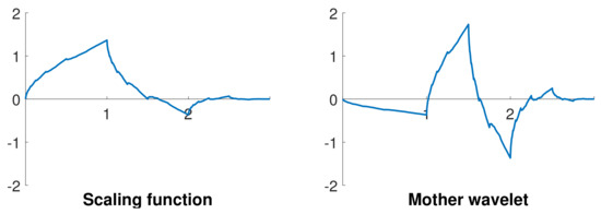
Figure 1. Scaling function and mother wavelet of the fourth-order Daubechies wavelet.

The down-sampling procedure after band-pass filtering at each wavelet decomposition stage reduces the signal resolution, which ignores minor signal responses and affects the identification of the interface locations from radargrams. Stationary wavelet transform (SWT) was designed to complement the translation-invariance, achieved by removing the down-samplers and up-samplers in the discrete wavelet transform and up-sampling the filter coefficients [48]. The signal size remains constant in the decomposition procedure. Keeping the signal size is significant, as the minimum recognizable scale is determined by the signal intervals. 2D SWT is appropriate for analyzing 2D datasets or pictures, as these signals have continuity in different orientations. The subsurface formations have both transverse and perpendicular continuities, and utilizing 2D SWT to interpret radargrams can reveal the horizontal relationships among diverse A-scan traces. The B-scan radargram is decomposed into multiple horizontal detail coefficients $D{H}_i$, vertical detail coefficients $D{V}_i$, diagonal detail coefficients $D{D}_i$ and approximation coefficients $A_i$, $i=1,2,\dots ,N$ (Equation (3)).

$$Y(x,t)=\sum _{i=1}^N(D{H}_i+D{V}_i+D{D}_i)+A_N,$$

(3)

where $Y(x,t)$ is the B-scan radargram and N is the decomposition number. In this research, we use the Matlab function ‘swt2’ for 2D SWT decomposition, and the sole parameter required is the fourth-order Daubechies wavelet.

2.3. F-K Migration

Frequency-wavenumber migration, or F-K migration, is an approach to convert hyperbola signals to object locations, firstly applied to process seismic signals [27]. It utilizes the exploding source model, where the scattered signal field is originated by the explosion at the object locations [49], to solve the wave equation (Equation (4)). F-K migration calculates the wave-field $\phi$ at $t=0$ when the explosion happens and the waves still locate at sources. The essence of F-K migration is the Fourier transform, which is derived from the general summation expression of a wave function (Equation (5)) [50].

$$(\frac{{\partial }^2}{\partial x^2}+\frac{{\partial }^2}{\partial z^2}-\frac{1}{v^2}\frac{{\partial }^2}{\partial t^2})\phi (x,z,t)=0$$

(4)

$$\phi (x,z,t)=\frac{1}{2\pi }{\int }_{-\infty }^{\infty }{\int }_{-\infty }^{\infty }\varphi (k_x,\omega )e^{-j(k_{x}x+k_{z}z-\omega t)}d{k}_{x}d\omega$$

(5)

where v is the propagation velocity (assumed constant in K-F migration) of electromagnetic waves, $k_x$ and $k_z$ are wave-numbers in the x and z directions, $\omega =v\sqrt{k_x^2+k_z^2}$ represents the frequency, and $\varphi$ is the Fourier transform from the surface field $\phi (x,0,t)$. $\phi (x,0,t)$ equals to the measured signal $Y(x,t)$ as GPR acquires the waves propagated to the surface. The target image is estimated by the initial wave-field $I(x,z)$ at $t=0$ (Equation (6)).

$$I(x,z)=\phi (x,z,0)=\frac{1}{2\pi }{\int }_{-\infty }^{\infty }{\int }_{-\infty }^{\infty }\varphi (k_x,\omega )e^{-j(k_{x}x+k_{z}z)}d{k}_{x}d\omega$$

(6)

By resampling $\varphi (k_x,\omega )$ to the $k_x-k_z$ domain, the migration results can be calculated by the inverse fast Fourier transform ${\mathcal{F}}^{-1}$ (Equation (7)). In this research, F-K migration is programmed by Matlab, and the parameter of propagation velocity can be calculated according to [25].

$$\begin{array}{c}\hfill I(x,z)={\mathcal{F}}_{k_x}^{-1}{\mathcal{F}}_{k_z}^{-1}\Phi (k_x,k_z)\\ \hfill \Phi (k_x,k_z)=\frac{v{k}_z}{\sqrt{k_x^2+k_z^2}}\varphi (k_x,v\sqrt{k_x^2+k_z^2})\end{array}$$

(7)

F-K migration is a linear function since the Fourier transform satisfies the linear superposition principle. The migration results of radargram can be regarded as the summation of migration from all SWT coefficients (Equation (8)).

$$M\left(Y(x,t)\right)=\sum _{i=1}^N(M\left(D{H}_i\right)+M\left(D{V}_i\right)+M\left(D{D}_i\right))+M\left(A_N\right),$$

(8)

where $M(·)$ represents the F-K migration function. The SWT coefficients have a good time-frequency resolution, and each component can contain clutter, targets, or hyperbola interference. Effective SWT signals containing the targets can enhance the migration results, while those occupied by clutter or hyperbola interference should be discarded. Thus the final target profile is reconstructed by selected migration components. Figure 2 presents the procedures of our proposed approach.

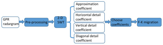
Figure 2. The flowchart of proposed methods.

2.4. Test Site

Field measurements were carried out in an underground cavern in Huangdao, China, before grouting reinforcement, with the measurement scheme shown in Figure 3a. The underground caverns were built inside the layer of granite for structural stability. We use the GPR instrument from ‘MALA-Geoscience’, moving along the cavern surface and transmitting 250 MHz electromagnetic waves into surrounding rock sections. The wave frequency is 250 MHz to reach the depth around 7 m. The measurement length of an example section is $0\le x\le 20$ m, and the time window is 130 ns. Figure 3b presents the original radargram. Since opening the rocks and obtaining the actual rock distribution are difficult, a finely processed radargram by expertise is used as ‘ground truth’ (Figure 3c).

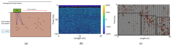
Figure 3. (a) A simple scheme of field measurements. (b) The original radargram. (c) The radargram processed by expertise.

3. Results

3.1. Simulated Signal Analysis

Scenario 1: identifying sparse rock cracks

Since visibly obtaining the actual fissure distribution inside the surrounding rocks is difficult, the numerically generated radargram is analyzed to compare the reconstructed profile with the preset geometric model. The open-source software, ‘gprMax’ [51], can simulate electromagnetic wave propagation inside the subterranean sections and have been extensively applied in evaluating GPR signal processing approaches (e.g., [52,53]). We assume that the signal reflections are all generated by rock fissures, not strata interfaces, since the underground caverns are built inside the single layer of granite. In this paper, we simulated the GPR signals from a subterranean area with the measurement length $0\le x\le$ 2 m and depth $0\le z\le$ 1 m. The subterranean material is granite with relative permittivity of 7 [54] and conductivity of 0.012 [55]. The model includes six horizontal 5 mm-thick cracks (the direction is limited by ‘gprMax’, vertically or horizontally) filled by air, as shown in Figure 4a. The simulated grid step is $▵x=▵z=0.005$ m, and the time window is 20 ns. GPR transmits an 800 MHz ricker wave and receives A-scan traces with 0.01 m intervals. The simulated radargram after pre-processing is presented in Figure 4b. The hyperbola tails in the radargram affect the visibility of crack sizes and locations.

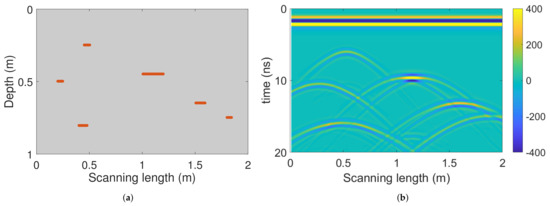
Figure 4. (a) Subterranean model with 6 cracks; (b) The pre-processed radargram.

Firstly, the radargram is decomposed by 2D SWT, and Figure 5 illustrates the 2nd layer coefficients for an example. The approximation coefficient is not considered in migration since it preserves both target signals and hyperbola tails similar to the pre-processed radargram. Vertical and diagonal detail coefficients only contain hyperbola tails, while hyperbola centers corresponding to cracks are invisible. These two coefficients are excluded for migration. The horizontal detail coefficient preserves the target signal and discards part of the hyperbola tails, suitable for further F-K migration. Therefore, only horizontal detail coefficients $D{H}_i$ in Equation (8) are considered in the migration step.

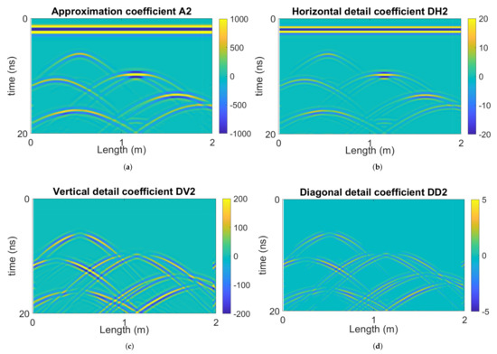
Figure 5. Second layer (a) approximation coefficient $A_2$, (b) horizontal detail coefficient $D{H}_2$, (c) vertical detail coefficient $D{V}_2$, and (d) diagonal detail coefficient $D{D}_2$.

The radargram is decomposed into four layers by 2D SWT. F-K migration processes the four horizontal detail coefficients and the pre-processed radargram for comparison, as shown in Figure 6. Without SWT decomposition, the migrated radargram (Figure 6e) highlights the crack locations, but preserves scattering signals, which are produced by hyperbola tails. Two-dimensional SWT has reduced the scatter in the migration results especially from the 3rd and 4th-layer horizontal coefficients (Figure 6c,d). However, when decomposing to deep SWT layers (e.g., 4th-layer in Figure 6d), the highlighted crack sizes increase. This is because the deep-layer signals have low frequency but large wavelengths. Therefore, $D{H}_3$ is more promising for avoiding scattering signals in migration and highlighting the crack locations and sizes. The radargrams contain artifacts marked in the dashed circles, which are unavoidable in all migration results. These artefacts are generated by multiple reflections between two upper cracks (center locations (0.52 m, 0.25 m) and (1.14 m, 0.45 m)).

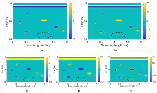
Figure 6. F-K migration results of (a) 1st-layer $D{H}_1$, (b) 2nd-layer $D{H}_2$, (c) 3rd-layer $D{H}_3$, (d) 4th-layer $D{H}_4$, and (e) pre-processed radargram without SWT decomposition.

Scenario 2: identifying sparse rock cracks from noisy environments

Noise is a significant issue affecting GPR signals. We add Gaussian white noise to the radargram to simulate the random noise. The same model in Figure 4a is utilized, and the polluted radargram (the signal-to-noise ratio is $-5$ db) is shown in Figure 7. Noisy speckles occupy the radargram, affecting the visibility of target signals and hyperbola tails.

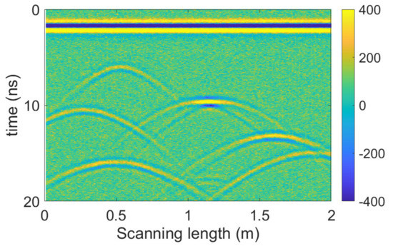
Figure 7. Polluted radargram of the model in Figure 4a.

The polluted radargram is decomposed into four layers by 2D SWT. Similar to scenario 1, only horizontal detail coefficients preserve target signals and mitigate part of hyperbola tails, as shown in Figure 8. The radargram is not decomposed into deeper layers that increase the crack sizes in the migration result. The coefficients $D{H}_1$ and $D{H}_2$ are occupied by noise, which means 2D SWT can separate noise out. $D{H}_3$ is a mixture of noise and target signals, unsuitable for crack identification. Noise nearly disappears in $D{H}_4$, and target signals become visible. Noise, target signals, and hyperbola tails have different time-frequency features, and therefore they can be separated by 2D SWT.

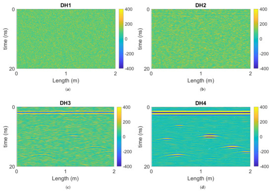
Figure 8. The horizontal detail coefficients of (a) 1st-layer $D{H}_1$, (b) 2nd-layer $D{H}_2$, (c) 3rd-layer $D{H}_3$, and (d) 4th-layer $D{H}_4$.

The F-K approach migrates the polluted radargram in Figure 7 and the 4th-layer $D{H}_4$, as illustrated in Figure 9. Although highlighting the crack locations, Figure 9a contains a similar noise level to Figure 7. Besides, scattering signals appear surrounding the focused locations in Figure 9a. The noise intensity decreases dramatically in Figure 9b since 2D SWT has separated the noisy layers. The migration result from $D{H}_4$ has highlighted the target locations and eliminated noise and hyperbola tails. However, the identified crack sizes increase due to the large wavelength in deep SWT layers.

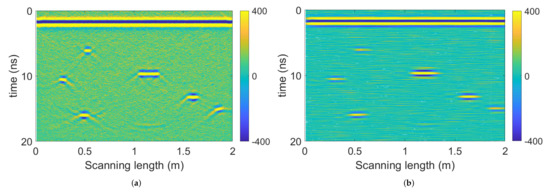
Figure 9. F-K migration results of (a) the polluted radargram and (b) the 4th-layer $D{H}_4$.

Scenario 3: identifying fractured rock areas with dense fissures

Fissure groups other than the single throughout crack are common in fractured rock areas. A subterranean area with the measurement length $0\le x\le$ 2 m and depth $0\le z\le$ 1 m is simulated by ‘gprMax’. There are three predefined fractured rock portions with rock fissures randomly distributed inside (fissure widths of 5 mm, lengths of 1–5 cm, and intervals of 1–5 cm), as shown in Figure 10a. Other model parameters are the same as scenario 1. Figure 10b illustrates the corresponding radargram after pre-processing. Dense hyperbola tails have occupied large subsurface areas, affecting the identification of fractured rock areas.

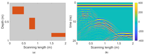
Figure 10. (a) Simulated subterranean area with three fractured rock portions ($0.1\le x\le 0.5$ m and $0.1\le z\le 0.3$ m; $0.7\le x\le 0.9$ m and $0.4\le z\le 0.7$ m; $1.5\le x\le 2$ m and $0.8\le z\le 0.9$ m). (b) The pre-processed radargram.

The radargram is firstly decomposed by 2D SWT, and Figure 11 illustrates the 2nd-layer coefficients for an example. Similar to scenario 1, the approximation coefficient contain both target signals and hyperbola tails. Vertical and diagonal detail coefficients only contain hyperbola tails, while hyperbola centers corresponding to fractured rocks are invisible. These coefficients are not considered for migration. The horizontal detail coefficient preserves target signals and mitigates part of the hyperbola tails. Therefore, only horizontal detail coefficients $DH$ are suitable for migration to identify the fractured rocks.

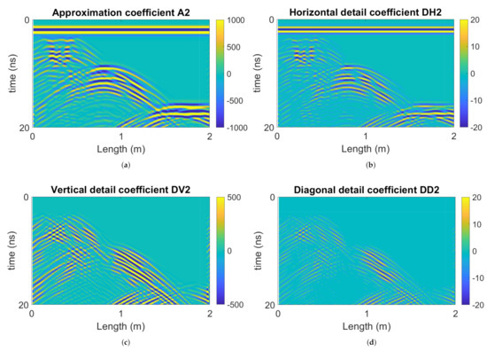
Figure 11. 2nd layer (a) approximation coefficient $A_2$, (b) horizontal detail coefficient $D{H}_2$, (c) vertical detail coefficient $D{V}_2$, and (d) diagonal detail coefficient $D{D}_2$ from 2D SWT on Figure 10b.

The radargram is decomposed into four layers by 2D SWT. F-K migration processes the four horizontal detail coefficients and the pre-processed radargram for comparison, as shown in Figure 12. Without SWT, scattering signals appear surrounding the fractured rocks highlighted in the migration result (Figure 12e). Migration from horizontal detail coefficients, especially of the deep layers, can mitigate the scattering signals. Artefacts (marked in the dashed circles) arising from multiple reflections also exist in the migration results, but SWT decomposition demonstrates potential to reduce this effect in $D{H}_3$ and $D{H}_4$. Different from scenario 1, the wavelength effect on identifying crack sizes is less significant when handling fractured rock areas. Limited by ‘gprMax’ software, the simulated cracks are horizontal, and $D{H}_3$ and $D{H}_4$ have revealed the horizontal directions of the cracks. Both $D{H}_3$ and $D{H}_4$ present promising results in highlighting the fractured areas and eliminating scattering signals.

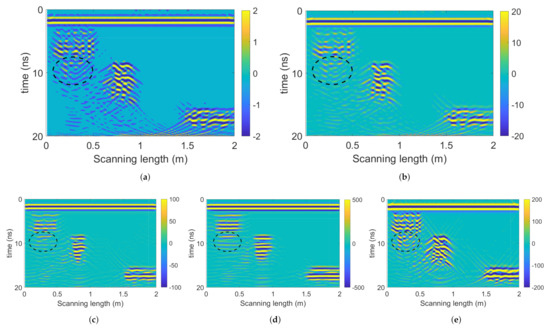
Figure 12. F-K migration results of (a) 1st-layer $D{H}_1$, (b) 2nd-layer $D{H}_2$, (c) 3rd-layer $D{H}_3$, (d) 4th-layer $D{H}_4$, and (e) pre-processed radargram without SWT decomposition.

Scenario 4: identifying fractured rock areas with dense fissures from noisy environment

Similarly, we consider the noise effect by adding Gaussian white noise to the radargram (Figure 10b), with the polluted profile (signal-to-noise ratio −5 db) shown in Figure 13. Noisy speckles occupy the radargram, affecting the visibility of target signals and hyperbola tails.

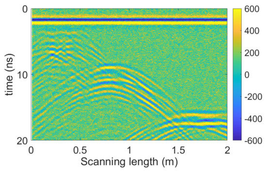
Figure 13. Polluted radargram of the model in Figure 10b.

The polluted radargram is decomposed into four layers by 2D SWT. Similar to previous scenarios, horizontal detail coefficients that preserve target signals and mitigate part of hyperbola tails are illustrated in Figure 14. The 2D SWT has separated noise to $D{H}_1$ and $D{H}_2$, and the noise nearly disappear in $D{H}_4$. Therefore, 2D SWT can distinguish noise, targets, and hyperbola tails.

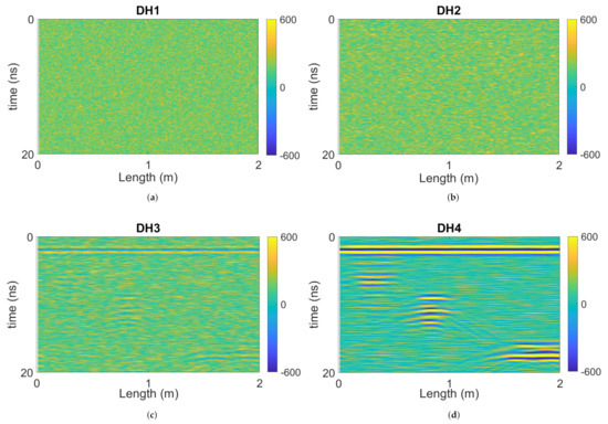
Figure 14. The horizontal detail coefficients of (a) 1st-layer $D{H}_1$, (b) 2nd-layer $D{H}_2$, (c) 3rd-layer $D{H}_3$, and (d) 4th-layer $D{H}_4$.

The F-K approach migrates the polluted radargram in Figure 13 and the 4th-layer $D{H}_4$, as illustrated in Figure 15. Although highlighting the crack locations, Figure 15a contains noise speckles polluting the crack signals and scattering signals appear surrounding the focused locations. The noise intensity decreases dramatically in Figure 15b since 2D SWT has separated the noisy layers. The migration result from $D{H}_4$ has highlighted the target locations and eliminated noise and hyperbola tails. Similar to scenario 3, the wavelength effect on crack lengths is little when handling fractured rock areas.

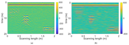
Figure 15. F-K migration results of (a) the polluted radargram and (b) the 4th-layer $D{H}_4$.

3.2. Field Signal Analysis

Figure 16 presents the pre-processed radargram from field measurement. Signals weaker than 2.5% of the maximum amplitude are excluded for better showing the fractured areas. These weak signals are mostly noise, which will not affect fractured rock identification but block the visible presentation from figures. The entire section is covered by intensive signals except for the upper-right portion (with the length $12\le x\le 17$ m and time $20\le t\le 65$ ns), which makes the fractured rocks indistinguishable.

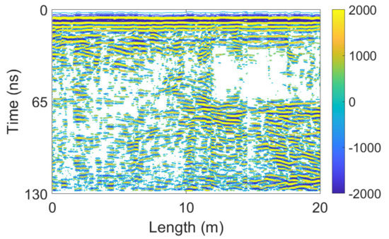
Figure 16. The pre-processed radargram from an example surrounding rock section. Signals weaker than 2.5% of the maximum amplitude are excluded.

Firstly, the pre-processed radargram is decomposed by 2D SWT, with the 2nd-layer coefficients shown in Figure 17. Similar to the simulation results, hyperbola tails have been decomposed to $D{V}_2$ and $D{D}_2$. The approximation coefficient presents similar distribution to the pre-processed radargram. Only $D{H}_2$ discards part of the noise and hyperbola tails, and preserves the target signals. Therefore, the horizontal coefficients are considered for further migration.

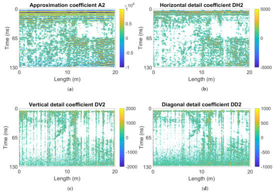
Figure 17. 2nd-layer coefficients from 2D SWT on Figure 16. (a) approximation coefficient $A_2$, (b) horizontal detail coefficient $D{H}_2$, (c) vertical detail coefficient $D{V}_2$, and (d) diagonal detail coefficient $D{D}_2$. Signals weaker than 2.5% of the maximum amplitude are excluded.

The F-K approach migrates $D{H}_1$, $D{H}_2$, $D{H}_3$, and the pre-processed radargram for comparison, as illustrated in Figure 18. The signals inside region U and the lower part of region V are weak in Figure 3c, but direct F-K migration preserves intensive signals (Figure 18d). This is affected by clutter. The 2D SWT can mitigate the clutter and thus the signals inside region U and the lower part of region V in Figure 18c become less intensive. Region W is identified as severely fractured rock areas. 2D SWT has demonstrated good practice in enhancing the migration results.

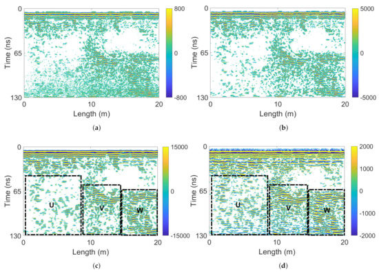
Figure 18. (a) F-K migration results of 1st-layer $D{H}_1$, (b) 2nd-layer $D{H}_2$, (c) 3rd-layer $D{H}_3$, and (d) pre-processed radargram without SWT decomposition. Signals weaker than 2.5% of the maximum amplitude are excluded.

4. Discussion

In this paper, a novel approach based on 2D WT and F-K migration is proposed to identify fractured rock areas from GPR radargrams. WT is theoretically similar to Fourier transform, the foundation of F-K migration, but alters the orthogonal basis. Therefore in signal processing, WT usually provides better time-frequency resolution [47]. By applying the proposed approach, three significant development has been achieved: (1) Noise, hy- perbola tails, and target signals are separated into different WT coefficients; (2) Scattered signals surrounding cracks in F-K migration results have been eliminated; (3) Noise has been mitigated in the focused radargram. The remained scattering energy in migrated profiles does not affect the identification of sparse objects (e.g., [44,56] and Figure 6e) and strata (e.g., [57]), but increases the identified crack group areas (Figure 12b) significantly. Therefore, eliminating the remained scattered signal is important for our application.

One phenomenon that arises from 2D WT is the wavelength effect. When identifying sparse cracks (Figure 6d and Figure 9b), the imaged crack length increases. The reason is that the wavelength increases as WT decomposes signals to deeper low-frequency components. Normally, the imaged crack size on an A-scan trace is influenced by the antenna frequency [58] (imaged size = wave-number × wavelength) and thus does not equal the actual size vertically. The 2D WT decomposes the radargram vertically and horizontally, and thereby the two-direction wavelengths vary in different decomposition layers. This results in the horizontal deformation of imaged cracks. To accurately calculate the object sizes, the frequency of processed radargram needs to compare with the antenna frequency vertically and with the original signal frequency horizontally. Nonetheless, the wavelength effect is little when identifying crack groups (Figure 12d) and thus affect little on our applications.

In our research, we apply 800 MHz waves in simulation and 250 MHz waves in field measurements. The choice of central frequency is determined by the required detection depth and resolution. The high-frequency electromagnetic waves have high resolution, but the energy attenuates quickly [25]. If using 250 MHz waves in simulation, the major difference is that the imaged cracks become thicker due to large wavelengths.

Our future researches will concern practical investigations of oblique and non-rectilinear rock fractures. The crack directions are limited by grids in numerical simulation and thus cannot cover all the crack conditions. In literature, long and throughout cracks (e.g., [59,60]) in different directions has been investigated in practical cases, but the conditions are not same as the fractured rocks. Although our approach can process radargrams from simulating other objects, including ‘cylinders’ and ‘spheres’, simulation of oblique and non-rectilinear rock fractures are impossible. Therefore, further researches should include more physical experiments to cover all the rock conditions.

The physical experiments are also important for validation since we cannot open the entire rock section in field measurements. The cracks or the fractured rock areas with different rock qualities can be preset, and thus our approach can be further evaluated. On this basis, we can establish the relationship between GPR radargrams and rock quality values in criterion.

5. Conclusions

In this paper, a novel approach based on 2D SWT and F-K migration is proposed to identify fractured rock areas from GPR radargrams. The 2D SWT can mitigate clutter, distinguish signal discontinuity, and provide signals with a good time-frequency resolution. It decomposes the radargram to different frequency levels and then feeds the signals into F-K migration. F-K migration can focus the scattered hyperbola signals back to the target locations. In practice, the detail coefficients achieved by 2D SWT can contain clutter, hyperbola tails, and target signals separately, and thus they are selected for the migration step.

The simulation and measurement results demonstrate that: comparing with direct F-K migration results, migration from the horizontal detail coefficients by 2D SWT can mitigate scattering signals and eliminate noise. 2D SWT decomposes the hyperbola tails to the vertical and diagonal detail coefficients, and separates the noise to the first few horizontal detail coefficients. Therefore, the corresponding migration results of later $DH$ highlight the crack locations and directions with little signal interference. The wavelength effect affects the identification of single cracks but not the crack groups. When decomposing to deep SWT layers, the frequency decreases and the wavelength increases. This results in the increased scale corresponding to the crack sizes. Nonetheless, the promising results indicate the effectiveness in identifying fractured rock areas. Future research will concern more practical cases since the simulations of oblique and non-rectilinear rock fractures are impossible.

References

- Deng, J.Q.; Yang, Q.; Liu, Y.R. Time-dependent behaviour and stability evaluation of gas storage caverns in salt rock based on deformation reinforcement theory. Tunn. Undergr. Space Technol. 2014, 42, 277–292. [Google Scholar] [CrossRef]
- Qiao, L.; Li, S.; Wang, Z.; Tian, H.; Bi, L. Geotechnical monitoring on the stability of a pilot underground crude-oil storage facility during the construction phase in China. Measurement 2016, 82, 421–431. [Google Scholar] [CrossRef]
- Khaledi, K.; Mahmoudi, E.; Datcheva, M.; Schanz, T. Stability and serviceability of underground energy storage caverns in rock salt subjected to mechanical cyclic loading. Int. J. Rock Mech. Min. Sci. 2016, 86, 115–131. [Google Scholar] [CrossRef]
- Deere, D.U. Technical description of rock cores for engineering purpose. Rock Mech. Eng. Geol. 1964, 1, 17–22. [Google Scholar]
- Zhang, L. Determination and applications of rock quality designation (RQD). J. Rock Mech. Geotech. Eng. 2016, 8, 389–397. [Google Scholar] [CrossRef]
- Yu, S.F.; Wu, A.X.; Wang, Y.M.; Li, T. Pre-reinforcement grout in fractured rock masses and numerical simulation for optimizing shrinkage stoping configuration. J. Cent. South Univ. 2017, 24, 2924–2931. [Google Scholar] [CrossRef]
- Kong, P.; Jiang, L.; Shu, J.; Sainoki, A.; Wang, Q. Effect of fracture heterogeneity on rock mass stability in a highly heterogeneous underground roadway. Rock Mech. Rock Eng. 2019, 52, 4547–4564. [Google Scholar] [CrossRef]
- Wang, L.; Chen, W.; Tan, X.; Tan, X.; Yang, J.; Yang, D.; Zhang, X. Numerical investigation on the stability of deforming fractured rocks using discrete fracture networks: A case study of underground excavation. Bull. Eng. Geol. Environ. 2020, 79, 133–151. [Google Scholar] [CrossRef]
- Yang, Y.W.; Bhalla, S.; Wang, C.; Soh, C.K.; Zhao, J. Monitoring of rocks using smart sensors. Tunn. Undergr. Space Technol. 2007, 22, 206–221. [Google Scholar] [CrossRef]
- Dai, F.; Li, B.; Xu, N.; Fan, Y.; Zhang, C. Deformation forecasting and stability analysis of large-scale underground powerhouse caverns from microseismic monitoring. Int. J. Rock Mech. Min. Sci. 2016, 86, 269–281. [Google Scholar] [CrossRef]
- Xu, N.W.; Li, T.B.; Dai, F.; Li, B.; Zhu, Y.G.; Yang, D.S. Microseismic monitoring and stability evaluation for the large scale underground caverns at the Houziyan hydropower station in Southwest China. Eng. Geol. 2015, 188, 48–67. [Google Scholar] [CrossRef]
- Zhao, J.S.; Feng, X.T.; Jiang, Q.; Zhou, Y.Y. Microseismicity monitoring and failure mechanism analysis of rock masses with weak interlayer zone in underground intersecting chambers: A case study from the Baihetan Hydropower Station, China. Eng. Geol. 2018, 245, 44–60. [Google Scholar] [CrossRef]
- Zhou, H.; Che, A. Geomaterial segmentation method using multidimensional frequency analysis based on electrical resistivity tomography. Eng. Geol. 2021, 284, 105925. [Google Scholar] [CrossRef]
- Park, B.; Kim, J.; Lee, J.; Kang, M.S.; An, Y.K. Underground object classification for urban roads using instantaneous phase analysis of ground-penetrating radar (GPR) data. Remote Sens. 2018, 10, 1417. [Google Scholar] [CrossRef]
- Porsani, J.L.; Jesus, F.A.N.D.; Stangari, M.C. GPR survey on an iron mining area after the collapse of the tailings dam I at the Córrego do Feijão mine in Brumadinho-MG, Brazil. Remote Sens. 2019, 11, 860. [Google Scholar] [CrossRef]
- Annan, A.P. Electromagnetic Principles of Ground Penetrating Radar. In Ground Penetrating Radar: Theory and Applications; Jol, H.M., Ed.; Elsevier: Oxford, UK, 2008; pp. 3–40. [Google Scholar]
- Kravitz, B.; Mooney, M.; Karlovsek, J.; Danielson, I.; Hedayat, A. Void detection in two-component annulus grout behind a pre-cast segmental tunnel liner using Ground Penetrating Radar. Tunn. Undergr. Space Technol. 2019, 83, 381–392. [Google Scholar] [CrossRef]
- Diamanti, N.; Redman, D. Field observations and numerical models of GPR response from vertical pavement cracks. J. Appl. Geophy. 2012, 81, 106–116. [Google Scholar] [CrossRef]
- Rasol, M.A.; Pérez-Gracia, V.; Fernandes, F.M.; Pais, J.C.; Santos-Assunçao, S.; Santos, C.; Sossa, V. GPR laboratory tests and numerical models to characterize cracks in cement concrete specimens, exemplifying damage in rigid pavement. Measurement 2020, 158, 107662. [Google Scholar] [CrossRef]
- Özdemir, C.; Demirci, Ş.; Yiğit, E.; Yilmaz, B. A review on migration methods in B-scan ground penetrating radar imaging. Math. Probl. Eng. 2014, 2014, 280738. [Google Scholar] [CrossRef]
- Kumlu, D.; Erer, I. Clutter removal in GPR images using non-negative matrix factorization. J. Electromagn. Waves Appl. 2018, 32, 2055–2066. [Google Scholar] [CrossRef]
- Ozdemir, C.; Demirci, S.; Yigit, E.; Kavak, A. A hyperbolic summation method to focus B-scan ground penetrating radar images: An experimental study with a stepped frequency system. Microw. Opt. Technol. Lett. 2007, 49, 671–676. [Google Scholar] [CrossRef]
- Jin, Y.; Duan, Y. A new method for abnormal underground rocks identification using ground penetrating radar. Measurement 2020, 149, 106988. [Google Scholar] [CrossRef]
- Stolt, R.H.; Weglein, A.B. Migration and inversion of seismic data. Geophysics 1985, 50, 2458–2472. [Google Scholar] [CrossRef]
- Jol, H.M. Ground Penetrating Radar Theory and Applications; Elsevier: Oxford, UK, 2008. [Google Scholar]
- Schneider, W.A. Integral formulation for migration in two and three dimensions. Geophysics 1978, 43, 49–76. [Google Scholar] [CrossRef]
- Stolt, R.H. Migration by Fourier transform. Geophysics 1978, 43, 23–48. [Google Scholar] [CrossRef]
- Cui, F.; Li, S.; Wang, L. The accurate estimation of GPR migration velocity and comparison of imaging methods. Geophysics 2018, 159, 573–585. [Google Scholar] [CrossRef]
- Feng, J.; Yang, L.; Xiao, J. Towards Metric GPR Migration based on DNN Noise Removal and Dielectric Estimation. arXiv 2021, arXiv:2104.10722. [Google Scholar]
- Busch, S.; van der Kruk, J.; Bikowski, J.; Vereecken, H. Quantitative conductivity and permittivity estimation using full-waveform inversion of on-ground GPR data. Geophysics 2012, 77, H79–H91. [Google Scholar] [CrossRef]
- De Coster, A.; Van der Wielen, A.; Grégoire, C.; Lambot, S. Evaluation of pavement layer thicknesses using GPR: A comparison between full-wave inversion and the straight-ray method. Constr. Build. Mater. 2018, 168, 91–104. [Google Scholar] [CrossRef]
- Jazayeri, S.; Kruse, S.; Hasan, I.; Yazdani, N. Reinforced concrete mapping using full-waveform inversion of GPR data. Constr. Build. Mater. 2019, 229, 117102. [Google Scholar] [CrossRef]
- Giannakis, I.; Giannopoulos, A.; Warren, C. A machine learning-based fast-forward solver for ground penetrating radar with application to full-waveform inversion. IEEE Trans. Geosci. Remote Sens. 2019, 57, 4417–4426. [Google Scholar] [CrossRef]
- Qin, H.; Tang, Y.; Wang, Z.; Xie, X.; Zhang, D. Shield tunnel grouting layer estimation using sliding window probabilistic inversion of GPR data. Tunn. Undergr. Space Technol. 2021, 112, 103913. [Google Scholar] [CrossRef]
- Pathak, R.S. The Wavelet Transform; Springer Science & Business Media: Paris, France, 2009. [Google Scholar]
- Smitha, N. Wavelet based clutter reduction of GPR data. In Proceedings of the 2017 International Conference on Circuits, Controls, and Communications (CCUBE), Bangalore, India, 15–16 December 2017. [Google Scholar]
- Baili, J.; Lahouar, S.; Hergli, M.; Al-Qadi, I.L.; Besbes, K. GPR signal de-noising by discrete wavelet transform. NDT E Int. 2009, 42, 696–703. [Google Scholar] [CrossRef]
- Tzanis, A. Detection and extraction of orientation-and-scale-dependent information from two-dimensional GPR data with tuneable directional wavelet filters. J. Appl. Geophy. 2013, 89, 48–67. [Google Scholar] [CrossRef]
- Zhan, R.; Xie, H. GPR measurement of the diameter of steel bars in concrete specimens based on the stationary wavelet transform. Insight 2009, 51, 151–155. [Google Scholar] [CrossRef]
- Kobayashi, M.; Uchikado, T.; Nakano, K. Wavelet-based position detection of buried pipes from GPR signals by use of angle information. In Proceedings of the 2012 International Conference on Wavelet Analysis and Pattern Recognition, Xi’an, China, 15–17 July 2012. [Google Scholar]
- Zhou, Y.; Chen, W. MCA-based clutter reduction from migrated GPR data of shallowly buried point target. IEEE Trans. Geosci. Remote Sens. 2018, 57, 432–448. [Google Scholar] [CrossRef]
- Feng, X.; Yu, Y.; Liu, C.; Fehler, M. Combination of H-alpha decomposition and migration for enhancing subsurface target classification of GPR. IEEE Trans. Geosci. Remote Sens. 2015, 53, 4852–4861. [Google Scholar] [CrossRef]
- Persico, R.; Morelli, G. Combined Migrations and Time-Depth Conversions in GPR Prospecting: Application to Reinforced Concrete. Remote Sens. 2020, 12, 2778. [Google Scholar] [CrossRef]
- Smitha, N.; Bharadwaj, D.U.; Abilash, S.; Sridhara, S.N.; Singh, V. Kirchhoff and FK migration to focus ground penetrating radar images. Int. J. Geo-Eng. 2016, 7, 1–12. [Google Scholar] [CrossRef]
- Szymczyk, M.; Szymczyk, P. Preprocessing of GPR data. Image Process. Commun. 2013, 18, 83. [Google Scholar] [CrossRef][Green Version]
- Bianchini Ciampoli, L.; Tosti, F.; Economou, N.; Benedetto, F. Signal processing of GPR data for road surveys. Geosciences 2019, 9, 96. [Google Scholar] [CrossRef]
- Mallat, S. A Wavelet Tour of Signal Processing; Elsevier: California, USA, 1999. [Google Scholar]
- Nason, G.P.; Silverman, B.W. The stationary wavelet transform and some statistical applications. In Wavelets and Statistics; Antoniadis, A., Oppenheim, G., Eds.; Springer: New York, NY, USA, 1995; pp. 3–40. [Google Scholar]
- Claerbout, J.F. Imaging the Earth’s Interior; Blackwell Scientific Publications: Oxford, UK, 1985. [Google Scholar]
- Stratton, J.A. Electromagnetic Theory; McGraw-Hill: New York, NY, USA, 1941. [Google Scholar]
- Warren, C.; Giannopoulos, A.; Giannakis, I. gprMax: Open source software to simulate electromagnetic wave propagation for Ground Penetrating Radar. Comput. Phys. Commun. 2016, 209, 163–170. [Google Scholar] [CrossRef]
- Jin, Y.; Duan, Y. Wavelet Scattering Network-Based Machine Learning for Ground Penetrating Radar Imaging: Application in Pipeline Identification. Remote Sens. 2020, 12, 3655. [Google Scholar] [CrossRef]
- Meşecan, İ.; Çiço, B.; Bucak, İ.Ö. Feature vector for underground object detection using B-scan images from GprMax. Microprocess. Microsyst. 2020, 76, 103116. [Google Scholar] [CrossRef]
- Hubbard, S.S.; Peterson, J.E., Jr.; Majer, E.L.; Zawislanski, P.T.; Williams, K.H.; Roberts, J.; Wobber, F. Estimation of permeable pathways and water content using tomographic radar data. Lead. Edge 1997, 16, 1623–1630. [Google Scholar] [CrossRef]
- Duba, A.; Piwinskii, A.J.; Santor, M.; Weed, H.C. The electrical conductivity of sandstone, limestone and granite. Geophys. J. Int. 1978, 53, 583–597. [Google Scholar] [CrossRef]
- Shen, R.; Zhao, Y.; Hu, S.; Li, B.; Bi, W. Reverse-Time Migration Imaging of Ground-Penetrating Radar in NDT of Reinforced Concrete Structures. Remote Sens. 2021, 13, 2020. [Google Scholar] [CrossRef]
- Vandenberghe, J.; Van Overmeeren, R.A. Ground penetrating radar images of selected fluvial deposits in the Netherlands. Sediment. Geol. 1999, 128, 245–270. [Google Scholar] [CrossRef]
- Luo, T.X.; Lai, W.W.; Chang, R.K.; Goodman, D. GPR imaging criteria. J. Appl. Geophy. 2019, 165, 37–48. [Google Scholar] [CrossRef]
- Theune, U.; Rokosh, D.; Sacchi, M.D.; Schmitt, D.R. Mapping fractures with GPR: A case study from Turtle Mountain. Geophysics 2006, 71, B139–B150. [Google Scholar] [CrossRef][Green Version]
- Zhang, L.; Xu, Y.; Zeng, Z.; Li, J.; Zhang, D. Simulation of Martian Near-Surface Structure and Imaging of Future GPR Data From Mars. IEEE Trans. Geosci. Remote Sens. 2021, 1–12. [Google Scholar] [CrossRef]
Publisher’s Note: MDPI stays neutral with regard to jurisdictional claims in published maps and institutional affiliations. |
© 2021 by the authors. Licensee MDPI, Basel, Switzerland. This article is an open access article distributed under the terms and conditions of the Creative Commons Attribution (CC BY) license (https://creativecommons.org/licenses/by/4.0/).