Article

Assessment of the Homogeneity of Long-Term Multi-Mission RO-Based Temperature Climatologies

1
Jiangsu Key Laboratory of Resources and Environmental Information Engineering, China University of Mining and Technology, Xuzhou 221116, China
2
School of Environment Science and Spatial Information, China University of Mining and Technology, Xuzhou 221116, China
3
Satellite Positioning for Atmosphere, Climate and Environment (SPACE) Research Centre, Royal Melbourne Institute of Technology (RMIT) University, Melbourne, VIC 3001, Australia
*
Author to whom correspondence should be addressed.
Remote Sens. 2021, 13(12), 2278; https://doi.org/10.3390/rs13122278
Submission received: 26 May 2021 / Revised: 5 June 2021 / Accepted: 7 June 2021 / Published: 10 June 2021
(This article belongs to the Section Atmospheric Remote Sensing)

Abstract

:
Atmospheric data obtained from the radio occultation (RO) technique are a well-recognized source of information for weather and climate studies. From the Challenging Minisatellite Payload (CHAMP) mission launched in July 2000 to the most recent Constellation Observing System for Meteorology, Ionosphere, and Climate follow-on (COSMIC-2) program, a continuous RO dataset of about 20 years has been collected, and a new opportunity for long-term climate analyses using multi-mission RO observations has subsequently arisen. Therefore, assessments of the long-term homogeneities of multi-mission RO data have become a necessary research task. For this purpose, in this study, we identified systematic discrepancies between the RO temperature profiles from the CHAMP, COSMIC, and Meteorological Operational Polar Satellite (METOP) missions. The results show that the temperature profiles from all three RO missions agree well in the upper troposphere and lower stratosphere (UTLS, 9–20 km altitude) regions, while some systematic discrepancies are found in the lower troposphere (2–8 km) and the high-altitude region (21–30 km). The homogeneities of long-term RO temperature climatologies were assessed by comparing them with radiosonde temperature records. The results of this comparison show obvious temporal inhomogeneities in the lower troposphere. The reasons for these temporal inhomogeneities include the systematic discrepancies between multi-mission RO profiles, the different monthly numbers of RO profiles, and the residual sampling error. The results of this study suggest that the systematic discrepancies between different RO missions should be thoroughly considered in the development of long-term multi-mission RO-based climatologies.

1. Introduction

As an active limb sounding technique, radio occultation (RO) was initially designed for detecting the atmospheric structures of Venus, Mars, and the outer planets, and it has been used for this purpose since the mid-l960s [1,2]. Its first application in the sounding of the Earth’s atmosphere was the proof-of-concept global positioning system/meteorology (GPS/MET) mission, which was launched in April 1995 and was active until February 1997. The GPS/MET instrument aboard the MicroLab-1 low Earth orbit (LEO) satellite receives signals transmitted from GPS satellites and refracted by the Earth’s atmosphere. The Doppler shifts of the refracted signals are accurately measured by atomic clocks aboard the LEO satellite, and the bending angle profiles, as a function of the so-called impact parameter, are then calculated using knowledge about the excess Doppler and occultation geometry. From the bending angle profiles, the atmospheric refractivity is derived using an Abel integral equation, and other atmospheric parameter values (e.g., atmospheric dry temperature, dry pressure, and dry density) can then be obtained based on the refractivity equation [3,4]:
N = 77.6 p T + 3.75 × 10 5 e T 2 4.03 × 10 7 n e f 2 + 1.4 W
where p and T are the atmospheric pressure and temperature in K and hPa, respectively; e is the partial pressure of watervapor in hPa; n e is the electron density in electrons/m3; f is the transmitter frequency in Hz; and W is the mass of condensed water in g/m3. Note that the last three terms on the right side of Equation (1) are neglected in the retrieval of dry parameters [5].
The primary achievement of the GPS/MET mission was to prove the feasibility of using the RO technique for sounding of the Earth’s atmosphere [6]. Following the success of the GPS/MET mission, several subsequent RO-related missions were launched, e.g., the Challenging Minisatellite Payload for geoscientific research (CHAMP); Constellation Observing System for Meteorology, Ionosphere, and Climate/Formosa Satellite Mission (COSMIC); and Meteorological Operational Polar Satellite (METOP) missions [7,8,9].
The RO technique can provide atmospheric data with all-weather capability, long-term stability, global coverage, and high accuracy and vertical resolution, factors that are important for weather and climate studies [10,11,12]. Owing to the limited lifetime of each single RO mission, RO data from a combination of multiple missions, rather than from a single mission, have been used for long-term climate studies. From early 2001 when the CHAMP mission became operational to the most recent COSMIC-2 program [13], an RO dataset covering a period of about 20 years has been developed. This provides the opportunity to use multi-mission RO data for relevant research and applications. However, because of the different characteristics of instrumental noise and signal-tracking methods applied for different RO missions, RO datasets from different missions may have systematic discrepancies, which can bring potential temporal inhomogeneities to RO-based climatologies. Therefore, it is necessary to investigate how best to use those multi-mission RO observations for climatological purposes as well as to evaluate the consistency and quality of long-term RO-based climatologies.
Several studies had been performed to evaluate the consistency and structural uncertainty of multi-mission RO climate data records. Foelsche et al. [14] investigated the consistency between RO-based refractivity and temperature records derived from different missions and concluded that the refractivity and dry temperature records from individual satellites with similar levels of bending angle noise can be safely combined for altitudes up to 30 km if the same data processing schemes are applied for all data. Steiner et al. [15] quantified the structural uncertainty of atmospheric trends estimated from the CHAMP RO records from six international RO processing centers. Their study showed that the regions that had the lowest RO structural uncertainty caused by different processing schemes are in the tropics and have mid-latitudes between altitudes of 8 and 25 km, while the uncertainty increases at altitudes above 25 km as well as at high latitudes. Angerer et al. [16] evaluated the consistency among various RO missions by calculating the deviations between the monthly mean temperature in RO data from different satellites and found a high level of consistency in the altitude range of 8 to 25 km, in which the deviations of the monthly mean temperature were less than 0.1 K. Steiner et al. [17] performed a rigorous intercomparison of a full set of RO data products from multiple satellites provided by different RO processing centers and found that all RO data products were highly consistent in the altitude range of 8 to 25 km, while more uncertainty was observed in CHAMP RO data at altitudes above 25 km. Gleisner et al. [18] evaluated the consistency of 15 years of climate data records from the CHAMP, Gravity Recovery and Climate, COSMIC, and METOP missions by comparing them with ERA-Interim reanalysis data. The results of the comparison suggest that the RO bending angle, refractivity, and dry temperature records show good overall agreement with the reanalysis at altitudes of 830 km, while large time-varying biases were observed for altitudes of 30–40 km and below 8 km. Similar investigations were also performed by Steiner et al. [19], Schreiner et al. [9], and Zhang et al. [20], and all of these studies confirmed the same finding: RO observations from different missions show a high level of consistency in the upper troposphere and lower stratosphere (UTLS) regions, while some systematic discrepancies are found in the lower troposphere and at high altitudes. However, the influences of systematic discrepancies in the RO-based climatologies are still unascertained and need further investigation, especially for long-term climatologies established based on RO profiles from different missions. For this purpose, in this study, taking atmospheric temperature as an example, the characteristics of the systematic discrepancies between RO profiles from different missions were analyzed, the potential temporal inhomogeneities in the long-term multi-mission RO-based temperature climatologies were identified, and the relationship between the temporal inhomogeneities and the systematic discrepancies was discussed.
The structure of this paper is outlined below. In Section 2.1, the datasets used in this study are introduced, including radiosonde data from the Integrated Global Radiosonde Archive (IGRA) dataset and RO temperature profiles delivered from the CHAMP, COSMIC, and METOP missions. Section 2.2 introduces the profile-to-profile comparison methods between co-located temperature profiles from RO and radiosonde as well as from different RO missions. The setup of RO- and radiosonde-based climatologies and sampling error estimation methods are presented in Section 2.3. Section 3.1 presents the profile-to-profile comparison results for each of the three missions, and the assessment of the homogeneity of the long-term multi-mission RO-based climatologies is presented in Section 3.2. A discussion of the reasons for the temporal mean shifts is presented in Section 4, followed by a summary and conclusions in Section 5.

2. Data and Methods

2.1. RO and Radiosonde Data

RO atmospheric profiles provided by the COSMIC Data Analysis and Archive Center (CDAAC) were used in this study. CDAAC provides three kinds of RO products: real-time, post-processed, and re-processed datasets. To ensure all RO profiles were processed by the same data retrieval methods and quality control schemes, only re-processed datasets were used in this study. The re-processed datasets contained RO profiles with various atmospheric variables on several product levels, e.g., atmospheric excess phase profiles (atmPhs file, level 1), dry atmospheric variable profiles (atmPrf file, level 2), and wet (physical) atmospheric variable profiles (wetPrf file, level 2). The wetPrf files, which represent the “real” state of the atmosphere, were adopted. Generally, the wet (physical) atmospheric temperature profiles of the re-processed datasets delivered from three RO missions, CHAMP, COSMIC, and Metop (Metop-A and Metop-B satellites), were used. A brief introduction for each of the missions is given below.
  • The CHAMP satellite was designed and managed by GeoForschungsZentrum Potsdam and launched into an almost circular orbit in July 2000 with an orbital altitude of 454 km and an inclination of 87.2°. The BlackJack RO receiver aboard the satellite, which was developed by NASA’s Jet Propulsion Laboratory (JPL), can track GPS L2 signals from which continuous RO observations can be obtained. From March 2001 to October 2008, the CHAMP satellite provided about 250 RO atmospheric profiles per day [21,22,23]. In this study, wet atmospheric temperature profiles from the CHAMP2016 re-processed dataset from 19 May 2001 to 26 July 2008 were used.
  • The COSMIC constellation consists of six LEO satellites and is a collaborative project of the Taiwan National Space Organization and the University Corporation for Atmospheric Research. The six satellites were first launched into their parking orbit at an altitude of 512 km in July 2006 and then gradually dispersed into their final orbits at an altitude of about 800 km and an inclination of 72° with an ascending node separation longitude of 30° (the FM-3 satellite was maintained at an orbit altitude of 711 km due to a solar array drive mechanism problem) [24]. All six satellites carry the Integrated GPS Occultation Receiver developed at the JPL, which tracks both setting and rising events. During its optimal working time (about 2007−2010), the COSMIC constellation provided more than 2000 atmospheric profiles per day [8,25], and in this study, we investigated the atmospheric profiles of the COSMIC2013 dataset collected for the period from 01 January 2007 to 31 December 2011.
  • The Metop series, operated by the European Organization for the Exploitation of Meteorological Satellite, is Europe’s first polar-orbiting operational meteorological satellite series and is dedicated to providing data for climate and environmental monitoring and the improvement of weather forecasting [26]. As the first and second satellites of the Metop series, Metop-A and Metop-B were launched into the Sun-synchronous orbit in October 2006 and September 2012 with orbital altitudes of 820 and 806 km, respectively, and with the same orbital inclination of 98.74°. Both satellites are equipped with a GNSS Receiver for Atmospheric Sounding, which can simultaneously track two rising and two setting RO events, providing about 700 RO events per day. In this study, we used the atmospheric profiles from the MetopA2016 and MetopB2016 datasets in the periods from 01 October 2007 to 31 December 2015 and from 01 February 2013 to 31 December 2015, respectively.
RO atmospheric profiles from the above three missions used in this study covered a 15-year period from 19 May 2001 to 31 December 2015. The monthly numbers for the RO profiles from each of the three missions are presented in Figure 1 (the monthly numbers for the RO profiles from the Metop-A and Metop-B satellites are shown separately). Note that only the profiles with good quality were used (i.e., the badness flag in CDAAC wetPrf file is equal to 0).
The radiosonde data from the IGRA-2 dataset, which were managed and maintained by the National Centers for Environmental Information in the United States, were used in this study. As the second version of the IGRA dataset, IGRA-2 provides historical and near-real-time radiosonde observations from around the globe, with various types of atmospheric data, including quality-assured individual soundings, monthly means, sounding-derived humidity, and station history information (at ftp://ftp.ncdc.noaa.gov/pub/data/igra, accessed on 15 November 2020). In this study, atmospheric temperature observations from the individual radiosonde soundings were used as a reference for the assessment of the homogeneity of multi-mission RO-based climatologies.
The IGRA-2 dataset provides radiosonde observations from more than 2000 radiosonde stations. As for the validation of radiosonde data, for any radiosonde station, at least 10 available observations per month were required for the period from May 2001 to December 2015 to ensure continuous and reliable monthly mean temperature data were available for the entire study period. Note that the monthly mean temperature directly provided by the IGRA was not adopted, because the monthly mean products contain sampling errors, which may contaminate comparison results (see Section 2.3 for more details).
Finally, a total number of 203 radiosonde stations remained, and Figure 2 illustrates their geolocations. Most of the stations are located in the Northern Hemisphere. Thus, the results from this study predominantly represent the climatologies in the Northern Hemisphere, especially in mid-latitude continental regions.

2.2. Profile-to-Profile Comparison Methods

To investigate the systematic discrepancies between the multi-mission RO temperature profiles, two comparison strategies were adopted in this study. First, the temperature profiles obtained from RO and nearby radiosonde stations were compared on a profile-to-profile basis. For the determination of a nearby radiosonde station and the validation of its data for comparison, a “collocation” matching criterion for both the spatial and temporal domains of the two datasets needed to be determined. Zhang et al. [20] and Gilpin et al. [27] showed the results of comparisons using different criteria (e.g., 100, 200, and 300 km spatial radial buffers combined with 1, 2, and 3 h temporal buffers), based on which the matching criteria of 300 km (spatial) and 3 h (temporal) were adopted in this study. It should be noted that, for an RO profile, if more than one radiosonde station is valid, all stations will be adopted. During the study period, a total of 183,984 pairs of radiosonde observations and co-located RO temperature profiles from the three missions were found to be valid for use in the comparison.
Before the comparison, the radiosonde profiles were mapped onto an altitude grid based on the geopotential height information reported for each pressure level [28]. The above pairs of profiles could not be directly compared as they are not at the same altitude levels; thus, both profiles needed to be interpolated to a common vertical grid. The two datasets have different resolutions in the vertical dimension: RO profiles have much smaller vertical intervals than radiosonde profiles, which are only reported at standard pressure levels. We should not simply interpolate the lower-resolution radiosonde data to the levels of the higher-resolution RO data, because a comparison following such an interpolation would produce small-scale features, which mainly reflect the structures of higher-resolution RO data instead of the real differences between the two types of observations. To overcome this problem, the methods suggested by Kuo et al. [21] and Gilpin et al. [27] were adopted. First, all of the valid profiles to be compared were linearly interpolated to uniform vertical grids with 0.1 km intervals. Then, a low-pass filter with a 1 km window size was applied to these interpolated profiles to remove the small-scale features in the RO profiles while preserving the overall structure of both the RO and radiosonde profiles. The filtered profiles were then linearly interpolated to the common vertical grids with 1 km intervals, and the interpolated profiles in the same vertical grid were compared, i.e., their differences were calculated (RO radiosonde).
In addition to the comparison between the RO and radiosonde profiles, an inter-comparison between the temperature profiles from different RO missions was also performed. First, the overlapping periods of the different RO missions were selected (i.e., periods containing RO observations from more than one mission), and the co-located profiles from the different RO missions were then collected with the same matching criterion (300 km and 3 h). Then, the differences between these co-located profiles were calculated. Information about the valid co-located RO profiles is presented in Table 1. The results of the two comparison strategies are presented in Section 3.1.

2.3. Setup of the Monthly Mean RO- and Radiosonde-Based Temperature Climatologies

The homogeneity of the long-term multi-mission RO-based climatologies was assessed by comparing them with radiosonde temperature climatologies. The following is a brief introduction to the setup of RO- and radiosonde-based climatologies.
The RO-based climatologies were calculated using the bin-and-average method, which was first introduced in the CHAMPCLIM project, which was dedicated to exploiting the CHAMP RO data for climate monitoring in the best possible manner [29,30,31]. RO profiles were gathered into geographical bins with a predefined spatial size and temporal duration. Then, the RO-based climatologies were calculated by averaging all of the RO profiles inside each bin (weighted with the cosine values of their latitudes). In this study, a spatial size of 10° × 10° (longitude/latitude) and a temporal duration of one month were predefined; then, geographical bins centered around each of the 203 radiosonde stations (as shown in Figure 2) with ±5° extensions in both the latitudinal and longitudinal directions were determined. The monthly mean RO-based temperature climatologies were then calculated by averaging the RO profiles in each bin using the common altitude grid with vertical intervals of 1 km.
The next step was to estimate the sampling error resulting from the uneven distribution of RO profiles in both the spatial and temporal domains. The above binning and averaging process skewed the averages toward the periods and regions where more profiles were observed [32,33]. The sampling error was estimated with the aid of background information. In this study, the 12 h forecasts from ECMWF were used as the background field [34] and these were used in the following way. First, the background field was interpolated to the times and geolocations of all RO profiles. Then, based on the obtained interpolated profiles, proxy RO-based climatologies were established using the same bin-and-average method. The estimated sampling error was then obtained by calculating the differences between the proxy climatologies and the background field. By removing the estimated sampling error from the RO-based climatologies, most of the influence of the sampling error was eliminated, leaving a residual sampling error that amounted to about 30% of the original one [35,36,37].
The radiosonde-based monthly mean temperature climatologies were calculated by averaging all individual radiosonde temperature observations in each month. The sampling error in the radiosonde temperature climatologies also needed to be estimated for the following reasons: (1) radiosonde data are a series of single-point measurements, whereas RO-based climatologies represent the mean atmospheric state of geographical bins; (2) generally speaking, radiosonde data are only collected twice per day (at around 00:00 and 12:00 UTC) and some data may even be unavailable or invalid due to both instrumental and artificial problems. Thus, although at least 10 observations are required per month for each station to determine the monthly mean, the mean value still does not reflect the true atmospheric state of the bins accurately, leading to a bias [27].
The sampling error in the radiosonde temperature climatologies was estimated using the same method as the one used for RO climatologies. The background information (ECMWF short-term forecast) was interpolated to the moment of the sounding data and the geolocation of the station, then the differences between the proxy climatologies (established based on the interpolated background temperature profiles) and the background field were used to calculate the estimated sampling error. After removing the estimated sampling error, the radiosonde-based climatologies represented the mean atmospheric state of the geographical bins centered around each of the radiosonde stations, thus a comparison could be performed. More details on the spatial–temporal sampling correction method for radiosonde climatologies can be found in the paper by Ladstadter et al. [38].

3. Results

3.1. Profile-to-Profile Comparison Results

3.1.1. Comparison between RO and Radiosonde

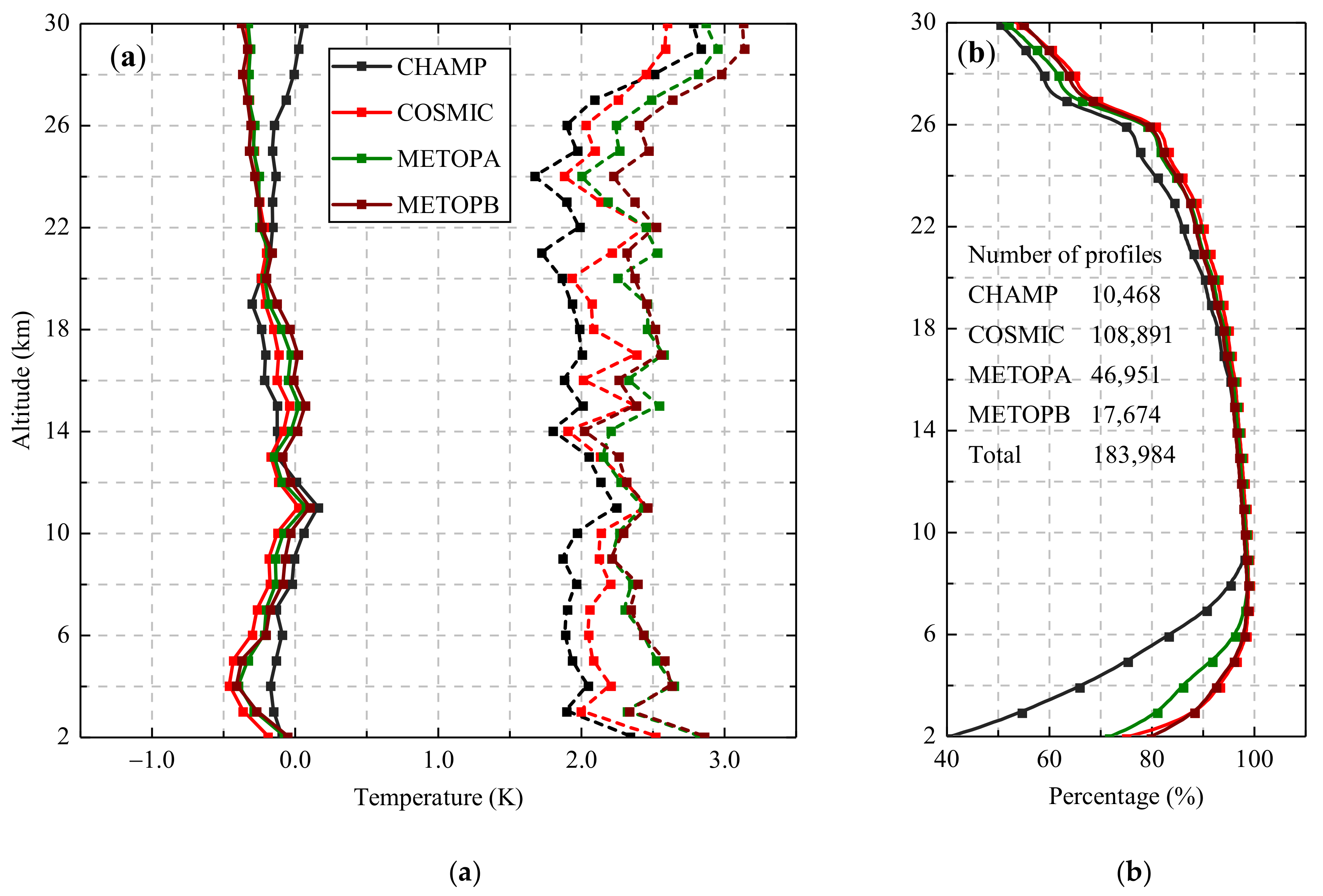
The statistical results of the differences between the temperature profiles from RO and nearby radiosonde stations are presented in Figure 3, including the mean and standard deviation of the differences and the proportion of available collocation profiles at different altitudes (from 2 to 30 km). Note that the RO temperature profiles that deviate from the radiosonde data by more than five times the standard deviations of the temperature differences were regarded as outliers; thus, they were discarded.
The data on proportions of valid collocation profiles show different characteristics depending on the mission (Figure 3b). The reason for this is twofold: first, because of the moist atmosphere in the lower troposphere and the surface topography, parts of RO profiles are terminated early before they penetrate the surface; in addition, the amount of available radiosonde data decreases with height, because radiosonde ascents often do not reach high altitudes. Under the comprehensive influences of the two factors, the proportions of available collocation profiles reach their maximum values at altitudes of around 69 km and decrease at higher and lower altitudes. Above 10 km, the proportions of the available collocation profiles for different missions show similar structures, and about 50–55% of the collocation profiles are still available at an altitude of 30 km, which mainly results from the absence of radiosonde observations. In the lower troposphere (2−8 km), the number of collocation profiles is mainly limited by the penetration depth of RO profiles. The proportions of the COSMIC and Metop collocation profiles show similar characteristics. Their numbers start to decrease at an altitude of about 7 km, and about 80% of the profiles penetrate to an altitude of 2 km (about 75% for COSMIC, 72% for Metop-A, and 81% for Metop-B, respectively). The number of CHAMP profiles starts to decrease from an altitude of about 9 km, and only about 40% of the collocation profiles penetrate to an altitude of 2 km. The main reason for this difference is that the COSMIC and Metop missions adopt the open-loop tracking technique, which substantially enhances the penetration depth of RO profiles in the lower troposphere [39,40].
As shown in Figure 3a, the mean of the differences between the collocation temperature profiles from the RO and radiosonde (named mean-differences profiles hereafter) demonstrate different characteristics depending on the altitude. According to the altitudinal characteristics, the vertical structures of the mean-differences profiles can be divided into three altitude ranges: the lower troposphere (2−8 km), the UTLS region (9−20 km), and the high-altitude region (21−30 km).
In the lower troposphere, the mean difference between the radiosonde and CHAMP RO profiles is very small, with most values being in the range of 0.2 to 0.1 K. For the COSMIC and Metop missions (both Metop-A and Metop-B satellites), the mean-difference profiles show similar structures. The difference is about 0.2 K at a 2 km altitude and a peak value of about 0.5 K is reached at an altitude of about 4 km, and then values decrease above this.
In the UTLS region, the mean-difference profiles of the COSMIC and Metop missions are similar at most altitudes, with values ranging from 0.3 to 0.1 K. The CHAMP profiles are about ± 0.2 K over the altitudes between 9 and 11 km; from altitudes of 12 to 20 km, their values are about 0.4 to 0.2 K.
In the high-altitude region, the mean difference among the three missions at an altitude of 21 km is about 0.2 K. The mean difference in the CHAMP profile is a decrease at altitudes up to 30 km, with most values being ± 0.2 K. The differences in the COSMIC and Metop profiles increase as the altitude increases, and the value at an altitude of 30 km is about 0.4 K.

3.1.2. Comparison between Different RO Missions

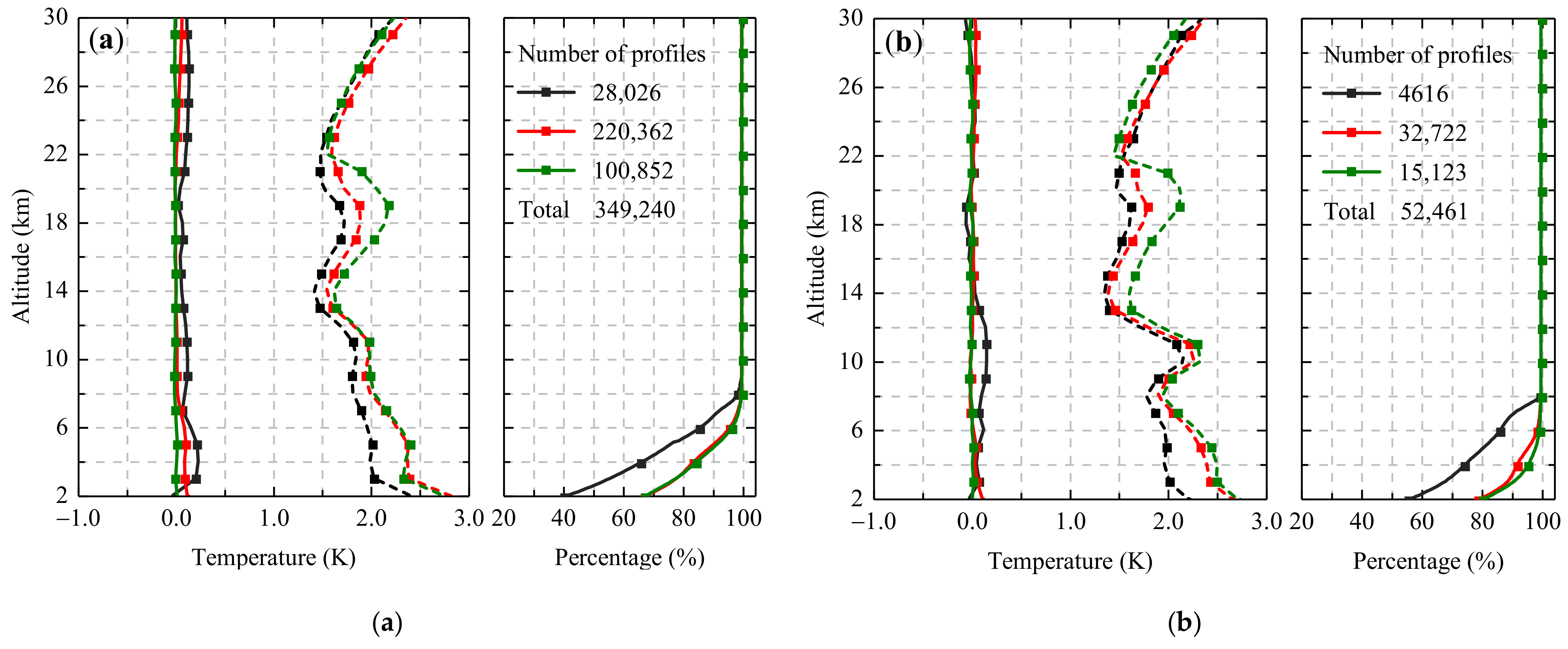
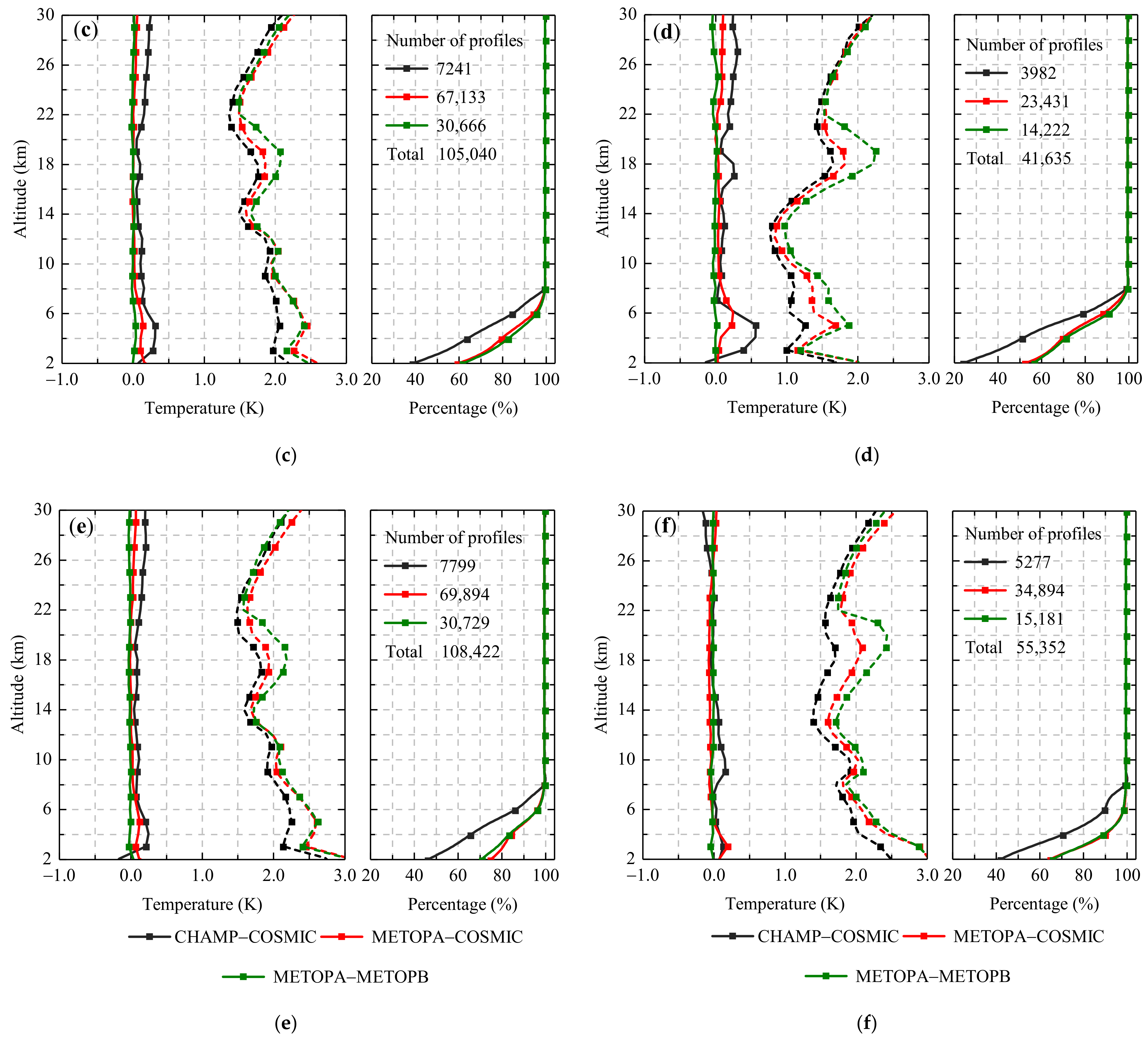
The statistical results of the temperature differences between multi-mission RO profiles in latitudinal bands of 90°S–90°N, 60°N–90°N, 20°N–60°N, 20°S–20°N, 60°S–20°S, and 90°S–60°S [41] are shown in Figure 4. Moreover, temperature profiles with more than five times the standard deviations of the differences were discarded.
As shown in Figure 4, the proportions of the valid co-located RO profiles are smallest at 2 km, reach their maximum values at about 6−9 km depending on the mission, and remain constant up to 30 km. The different proportions mainly result from the different penetration depths of the RO profiles from different missions, as mentioned in Section 3.1.1.
The means and standard deviations of the temperature differences at altitudes of 4, 14, and 26 km are summarized in Table 2. Based on Table 2 and Figure 4, the systematic differences between the multi-mission RO temperature profiles were identified at different latitudinal bands.
  • CHAMP COSMIC. In the high latitude region (60°N–90°N and 90°S–60°S, Figure 4b,f), between 2 and 15 km, the temperature differences between the CHAMP and COSMIC missions are very small at an altitude of 2 km and increase with height, reaching their peak value of about 0.2 K at 9–11 km before decreasing at higher altitudes. Between 15 and 25 km, the difference is less than 0.1 K, and above 25 km, small negative differences are observed, with the minimum values being about −0.2 K in the Southern Hemisphere. At latitudes between 20°N/S and 60°N/S (Figure 4c,e), the temperature difference is about 0–0.1 K at an altitude of 2 km. This increases as the altitude increases, reaches a maximum value of about 0.3 K at 4 km, and then decreases to an altitude of 8 km. At altitudes between 9 and 20 km, the differences are dominated by positive values with values varying from 0 to 0.1 K; above 20 km, the differences increase as the altitude increases, reaching about 0.2 K at 26 km. In the tropical band (20°S–60°N, Figure 4d), large positive differences are observed below 7 km, reaching a maximum value of about 0.6 K. At altitudes between 8 and 20 km, most of the temperature differences are within the range of 0–0.1 K. Above 20 km, the differences increase with altitude, and the maximum difference is about 0.3 K at around 26 km.
  • Metop-A COSMIC. In the middle and high latitude regions (20°N/S–90°N/S, Figure 4b–f), the differences between Metop-A and COSMIC are dominated by positive values over 2–8 km, with values varying between 0.1 and 0.2 K. Above an altitude of 8 km, the differences fall into the range of 0–0.1 K. In the tropical band, the temperature difference is about −0.1 K at 2 km. It reaches its maximum at 5 km with a value of about 0.3 K and then decreases as the altitude increases to 9 km. At altitudes between 10 and 20 km, the difference is 0.1 K. At altitudes above 20 km, the difference increases as the altitude increases and reaches a maximum of about 0.15 K at 30 km.
  • Metop-A Metop-B. The mean-difference profiles between the Metop-A and Metop-B missions show similar structures in six latitudinal bands. Their values maintain high consistency at most altitude levels, with most values ± 0.1 K.
    Overall, the temperature profiles from the COSMIC and Metop missions show good agreement for most altitudes, while noticeable discrepancies can be observed for CHAMP temperature profiles, especially in the lower troposphere.

3.2. Comparison between RO- and Radiosonde-Based Climatologies

The deseasonalized RO- and radiosonde-based temperature climatologies are calculated using:
T i Deseason h , s , t   =   T i h , s , t     T i ¯ h , s , m
where s , h , and t are the indices of the monthly mean temperature series for each station ( s = 1 ,   2 ,   3 ,   ,   203 ), altitude (   h = 2 ,   3 ,   4 ,   ,   30   km ), and month in the period from May 2001 to December 2015 ( t = 1 ,   2 ,   3 ,   ,   176 ). m is the ordinal number of the month ( m = 1 ,   2 ,   3 , ,   12 ); i is the index of the RO or radiosonde data; T i h , s , t is the monthly mean temperature of the RO- or radiosonde-based temperature climatologies; T i ¯ h , s , m is the mean annual temperature cycle, which is calculated by averaging all mean temperatures for a particular month ( m ) over all available years [15,17,42].
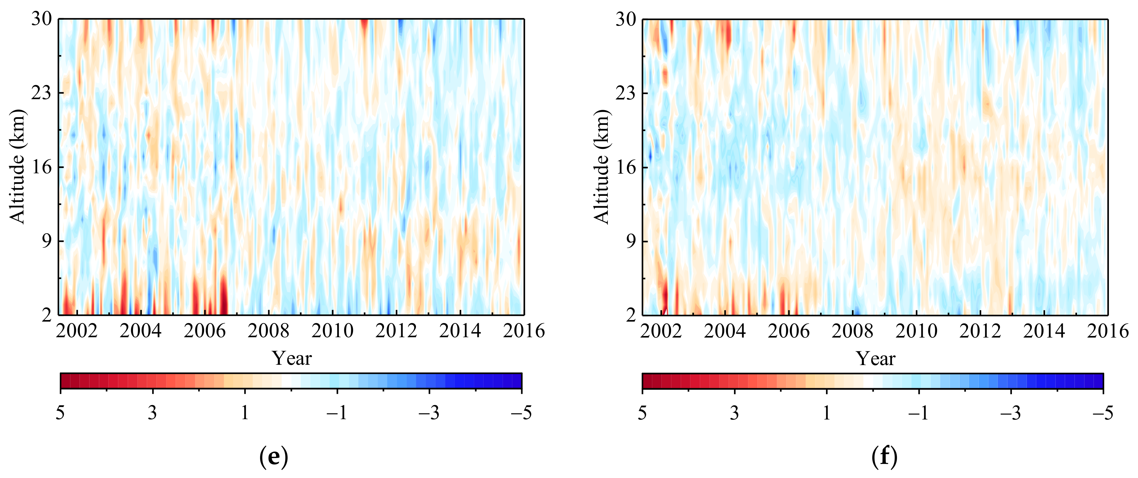
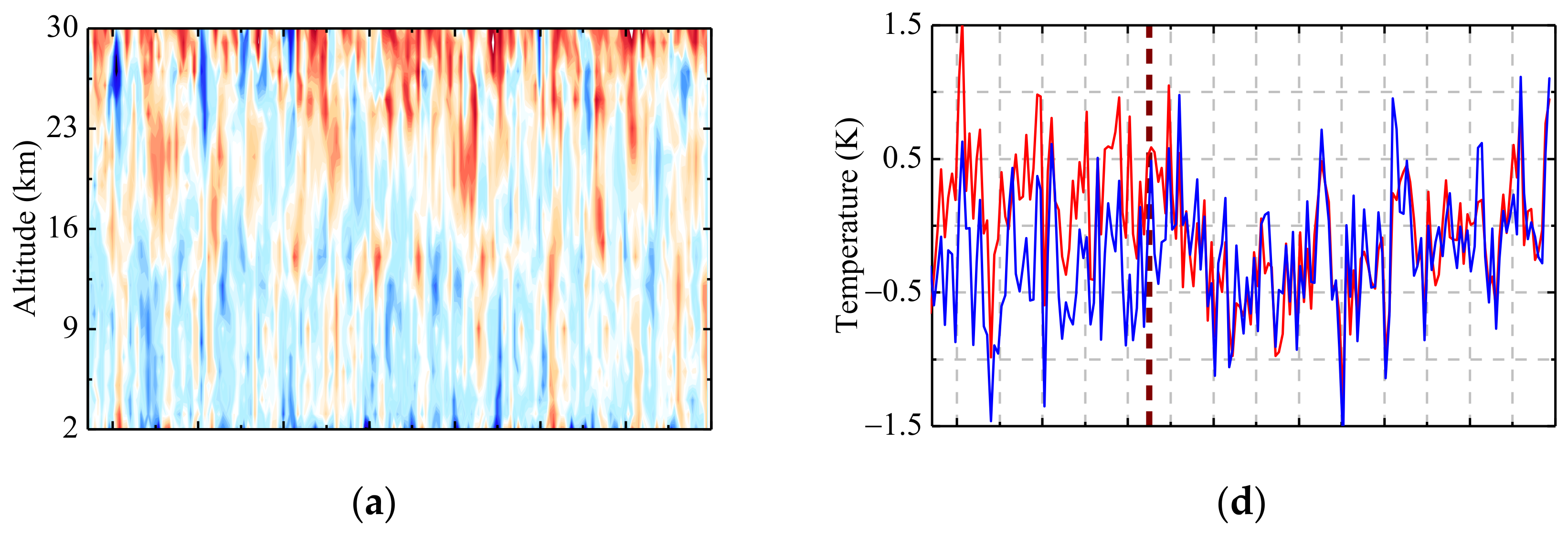
For an initial overview, the deseasonalized RO- and radiosonde-based temperature climatologies at two selected radiosonde stations, Hamamatsu AB in Japan (station ID: JAM00047681, 34.75°N/137.70°E) and Brownsville/INT in the US (station ID: USM00072250, 25.92°N/97.41°W), were determined, and the differences between the climatologies (i.e., RO radiosonde) at the two stations are presented in Figure 5.
The differences between the RO- and radiosonde-based deseasonalized temperatures show different characteristics at various altitude levels (Figure 5e,f). In the lower troposphere, the differences over the period from 2001 to 2006 are dominated by positive values and have large variability with a maximal value of about 5 K. From 2007 to 2015, the values of the differences are about ±1 K. In the UTLS region, the differences are relatively small, with most values being ±1 K. In the high-altitude region, the differences show a similar temporal structure to that of the lower troposphere, but with smaller magnitudes.
For more confirmative results, the means of the RO- and radiosonde-based deseasonalized temperature climatologies at all 203 stations were calculated. Based on the altitudinal characteristics of the temperature differences, the layer-average deseasonalized temperature series for either RO- or radiosonde-based climatologies in each of the three altitude ranges (the lower troposphere, the UTLS region, and the high-altitude region) were calculated by
T i , j Deseason s , t   = 1 n levels H 1 H 2 T i Deseason h , s , t
where and have the same descriptions as in Equation (2); is the index for the altitude range ( j = 1 ,   2 ,   3 ); and H 1 , H 2 , and n levels are the lower boundary ( H 1 = 2 ,   9 ,   21   km ), the upper boundary ( H 2 = 8 ,   20 ,   30   km ), and the number of altitude levels in each of the three altitude ranges ( n levels = 7 ,   12 ,   10 ).
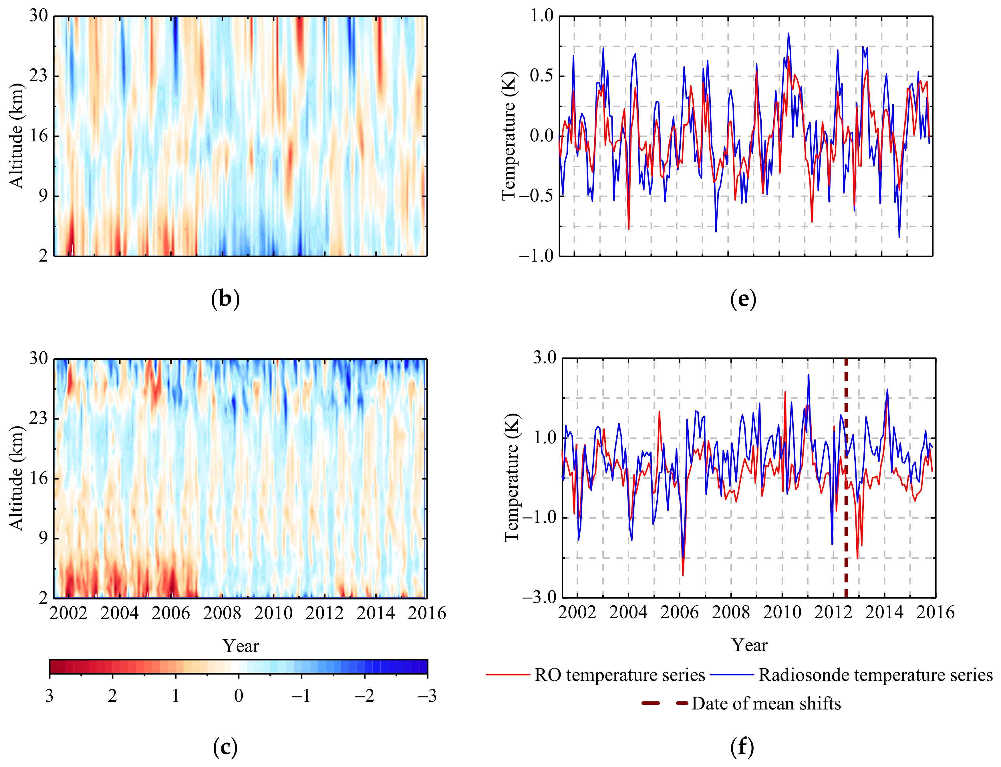
The mean values of the RO- and radiosonde-based deseasonalized temperature climatologies at the 203 stations are presented in Figure 6, as well as the layer-average series for each of the three altitude regions.
The RO- and radiosonde-based temperature climatologies show different characteristics in different altitude ranges. In the lower troposphere, obvious negative mean shifts can be observed for the RO-based temperature climatologies around the end of 2006 (Figure 6b), while similar phenomena are not present in the radiosonde-based climatologies (Figure 6a). For data from around the middle of 2012, small positive mean shifts can be observed for the RO-based temperature climatologies. Similar phenomena can be observed for the radiosonde-based climatologies, but with smaller magnitudes. In the UTLS region, both the RO- and radiosonde-based temperature climatologies stay consistent over the period from 2001 to 2012, while small positive mean shifts of about 0.5 K can be observed around the beginning of 2013. In the high-altitude region, the radiosonde-based temperature climatologies are dominated by positive values, with the maximum being about 3 K. For the RO-based climatologies, the deseasonalized temperature falls in the range of about −1.5 to 1.5 K.
For the layer-average deseasonalized temperature series (Figure 6d–f), the overall structures of the RO- and radiosonde-based series were found to be well-matched, indicating that RO temperature observations can capture the main features of atmospheric variability. However, some temporal mean shifts were still observed. For example, in the lower troposphere, the differences between the RO- and radiosonde-based series range from about 0.5–1 K to about 0–0.5 K at around April 2006 (Figure 6e); in the high altitude region, from 2001 to 2012, the RO-based temperature series are basically consistent with the radiosonde-based series, while obvious negative mean shifts of about 1 to 0.5 K can be observed around March 2012 (Figure 6f).
To further investigate the characteristics of the temporal mean shifts in the RO-based temperature climatologies, we detected changepoints (i.e., the beginning of the mean shift) in all deseasonalized RO temperature series using the penalized maximum t test (PMTred) algorithm with a level of confidence of 0.99. The radiosonde series was used as the reference to remove the trend term, natural variability terms, residual seasonal term, and other components that may influence the detection power of the PMTred method. Details on the PMT algorithm and the multiple mean shifts detection method can be found in Wang et al. [43] and Wang [44]. As a result, in the series of 5887 (203 stations and 29 altitude levels from 2 to 30 km with a vertical interval of 1 km), 1901 mean shifts were detected, with 660, 601, and 640 of them being in the lower troposphere, the UTLS region, and the high-altitude region, respectively. The statistical results for the mean shift in each of the altitude ranges are listed in Table 3.
Table 3 indicates that 73.5% of the RO deseasonalized temperature series can be declared homogeneous at the nominal level of confidence of 0.99 (i.e., with no mean shifts detected). The homogeneous series proportion is the smallest in the lower troposphere (61.8%) and the largest in the UTLS region (80.1%), which is consistent with the conclusions of previous studies showing that the RO-based climatologies are most consistent in the UTLS region [17,42].

4. Discussion

4.1. Analysis of the Reasons for Temporal Mean Shifts in RO-Based Climatologies

4.1.1. Inhomogeneities in Radiosonde-Based Climatologies

The reasons for the detected temporal mean shifts in the RO-based climatologies are multi-fold. First, the radiosonde-based climatologies were used as a reference field in changepoint detection using the assumption that the radiosonde temperature series were homogeneous over the study period. However, this assumption is not valid in practice. The performance of the radiosonde observations is influenced by the instrumentation and observation practices carried out at radiosonde stations, and changes in instruments and observation practices (e.g., changes in computing systems, radiation correction, and radiosonde model) may introduce systematic discrepancies to the radiosonde observations as well as potential temporal inhomogeneity in the radiosonde temperature series. Therefore, the radiosonde time series cannot be considered homogeneous over the whole study period, and the detected temporal mean shifts may result from the reference field (radiosonde-based climatologies) instead of the tested field (RO-based climatologies).
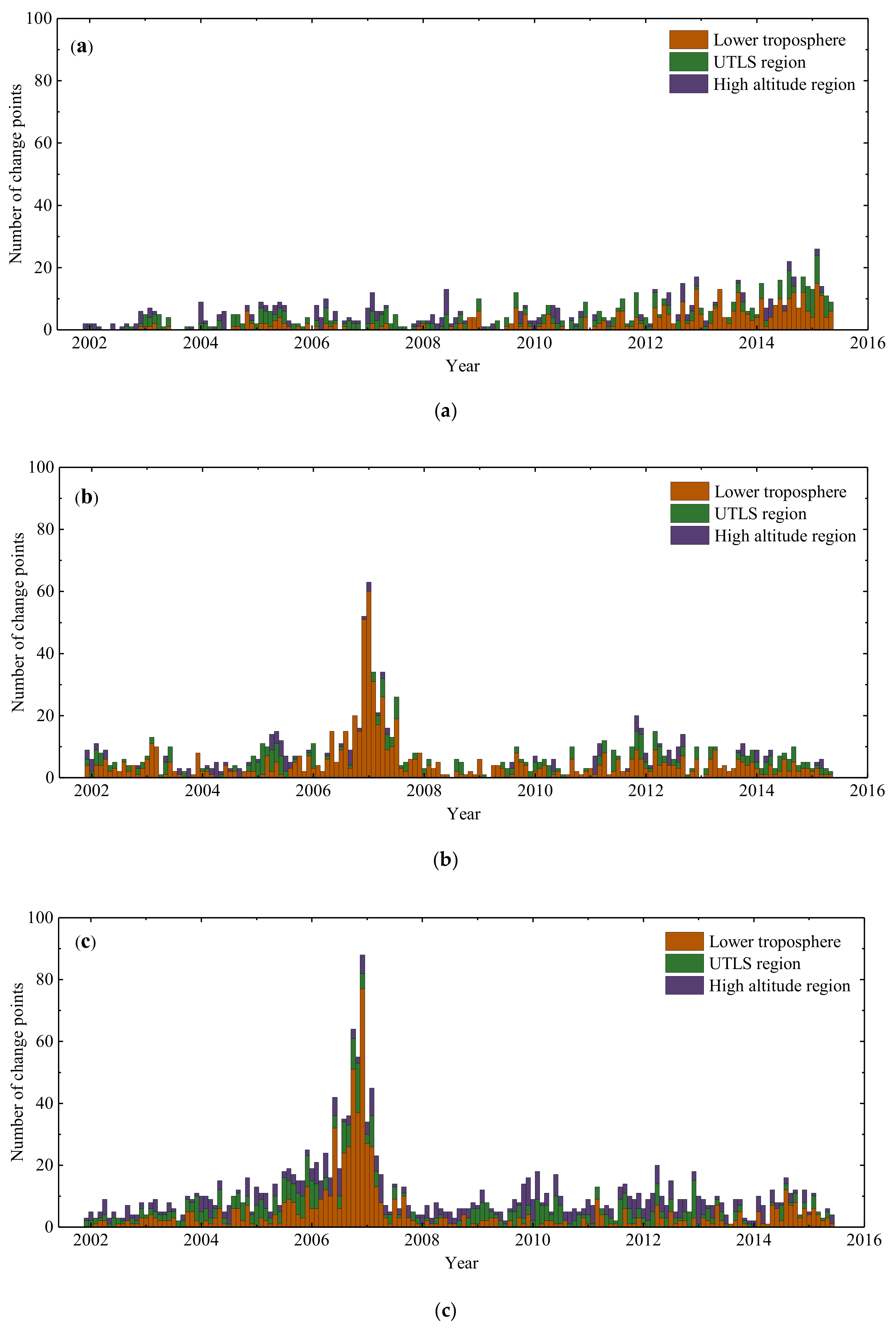
To investigate the influences of the reference field on the detection result, the changepoints in the reference field and tested field were detected independently using the PMTred method (i.e., detected without any reference), also at the nominal level of confidence of 0.99. The monthly numbers of detected changepoints for both the reference and tested fields are presented in Figure 7.
As shown in Figure 7a, in the high-altitude region, the monthly numbers of changepoints for the reference field were generally less than 10 per month. In the lower troposphere and the UTLS region, the monthly number remained consistent from 2001 to 2011, with most values being less than 10. From about March 2012, the monthly number started to increase and reached its maximum (about 20 and 10 changepoints per month for the lower troposphere and the UTLS region, respectively) in February 2015.
The monthly number of change points in the test field is shown in Figure 7b. In the lower troposphere, the detected changepoints were mainly concentrated in the period from August 2006 to May 2007, with the maximum value being about 60 per month. In the UTLS and the high-altitude region, the monthly numbers stayed consistent throughout the study period, with most values being less than 10 per month.
Figure 7c shows the monthly number of changepoints in the RO-based climatologies, with the radiosonde field being used as a reference for changepoint detection. The histograms highlight one significant singularity located around the period from August to November 2006, during which the monthly number of changepoints was more than 40 and most of these changepoints were observed in the lower troposphere. In this period, a large number of changepoints were also detected in the test field (RO-based climatologies, Figure 7b). Meanwhile, most of the temperature series in the reference field (radiosonde-based climatologies, Figure 7a) were declared homogeneous. Thus, the influence of the reference field on the changepoint detection results was very limited during this period.

4.1.2. Systematic Discrepancies between the Multi-Mission RO Temperature Profiles

The second factor that may influence the homogeneity of the RO-based climatologies is the systematic discrepancies between the temperature profiles from different RO missions. As shown in Figure 7c, many changepoints were detected at the end of 2006, and these coincided with the moments at which COSMIC profiles became available in the RO dataset. Based on the statistical results for the changepoints in the RO temperature climatologies and the knowledge of systematic discrepancies between the temperature profiles from the three RO missions (presented in Section 3.1), the influences of the systematic discrepancies on the multi-mission RO-based climatologies were analyzed.
From May 2001, the CHAMP RO profiles were the only data source for information on RO climatologies until the COSMIC profiles were introduced in January 2007. As the COSMIC mission produces colder temperature profiles than the CHAMP mission, the RO-based climatologies become colder after being assimilated with the COSMIC profiles (Figure 6b), subsequently leading to a negative mean shift in the temperature difference (Figure 6c).
It should be noted that the systematic discrepancies between the multi-mission RO profiles not only result from the instrumental noise and signal-tracking methods applied for each mission, but are also associated with the a priori/background information used in RO data retrieval processes. In this study, data on the physical RO atmospheric temperature, which were retrieved using the 1D-Var algorithm with the help of a priori information (e.g., ECMWF reanalysis), were used as the experimental data. The quality of the physical RO temperature is influenced by the priori information, especially in the lower troposphere where most of the atmospheric water vapor is present [45]. Therefore, upgrades or changes to the priori information may introduce systematic discrepancies to the physical temperature data as well as potential temporal inhomogeneity in the RO temperature series, e.g., a major upgrade was implemented at the ECMWF in February 2006 involving increases in the vertical and horizontal resolutions and an increase in the model top [46].
A similar situation occurs in the high-altitude region. As RO profiles are usually unavailable at high altitudes (>80 km), high-altitude initialization information (bending angle) is needed to conduct the inverse Able transform as a process of RO data retrieval. Thus, bad quality initialization information results in errors in the RO refractivity profiles, subsequently leading to misleading temperature, density, and pressure results. In addition, at high altitudes, where the signal-to-noise ratio becomes very small, the retrieval bending angles are more sensitive to noise, such as residual ionospheric noise and receiver thermal noise. A statistical optimization method can thus be used to obtain the most probable bending angles by combining the observed profiles with background information (e.g., MSIS model output) in a statistically optimal way [47]. Thus, the changes or improvements in the background information are also a possible reason for the detected temporal mean shifts.

4.1.3. Residual Sampling Error and Different Numbers of RO Profiles

In addition to the above two reasons, other factors that may influence the homogeneity of the RO-based climatologies and the results of the changepoint detection are presented below.
The residual sampling error. The residual sampling error exists in both the RO- and radiosonde-based temperature climatologies. For RO-based climatologies, the sampling error is influenced by the distribution of RO profiles in both space and time domains and mainly depends on the orbital elements of LEO satellites. Thus, as the data sources have changed over time, inconsistently distributed RO profiles usually result in sampling errors with different features and magnitudes, subsequently leading to varying residual sampling errors over the study period.
For the radiosonde-based climatologies, the single-point radiosonde observations were transformed to the mean atmospheric state of geographical bins using the spatial−temporal sampling correction method, as mentioned in Section 2.3. The sampling error of radiosonde-based climatologies is associated with the distribution of radiosonde profiles. The locations of radiosonde observations can generally be considered consistent over time. However, the moments of these observations are changeable, and the unavailable or invalid observations for each station also influence the sampling error and residual sampling error of radiosonde-based temperature climatologies.
As the values and distributions of the residual sampling error cannot be accurately estimated, it is difficult to carry out an accurate evaluation of its influences on the investigated homogeneity. However, the influence should be very limited, because the magnitude of the residual sampling error is very small. For example, for the Brownsville/INT station (Section 3.2), the estimated sample error for the RO-based climatologies is between −0.5 and 0.5 K most of the time (not shown), so the magnitude of the residual sampling error is about 0.15 K (accounting for 30% of the original value).
The different numbers of RO profiles collected over the study period. Because of the different numbers of RO profiles delivered from the three missions, the monthly number of RO profiles shows large variability over the study period. For example, the monthly number of profiles was less than 10,000 before 2007 when CHAMP was the only data source, while the number increased to 70,000 between 2007 and 2010 when COSMIC profiles were assimilated (Figure 1). The lack of RO profiles weakens the robustness of the bin-and-average method and leads to general degradation of the quality of the RO-based climatologies, especially in the lower troposphere where parts of RO profiles are unavailable because of the penetration depths required. This can also explain the large short-term variability in the RO-based climatologies between 2001 and 2006 (Figure 5 and Figure 6) when CHAMP RO profiles were the only data source.

4.2. Influences of the Temporal Mean Shifts on the Application of RO-Based Climatologies in Climate Studies

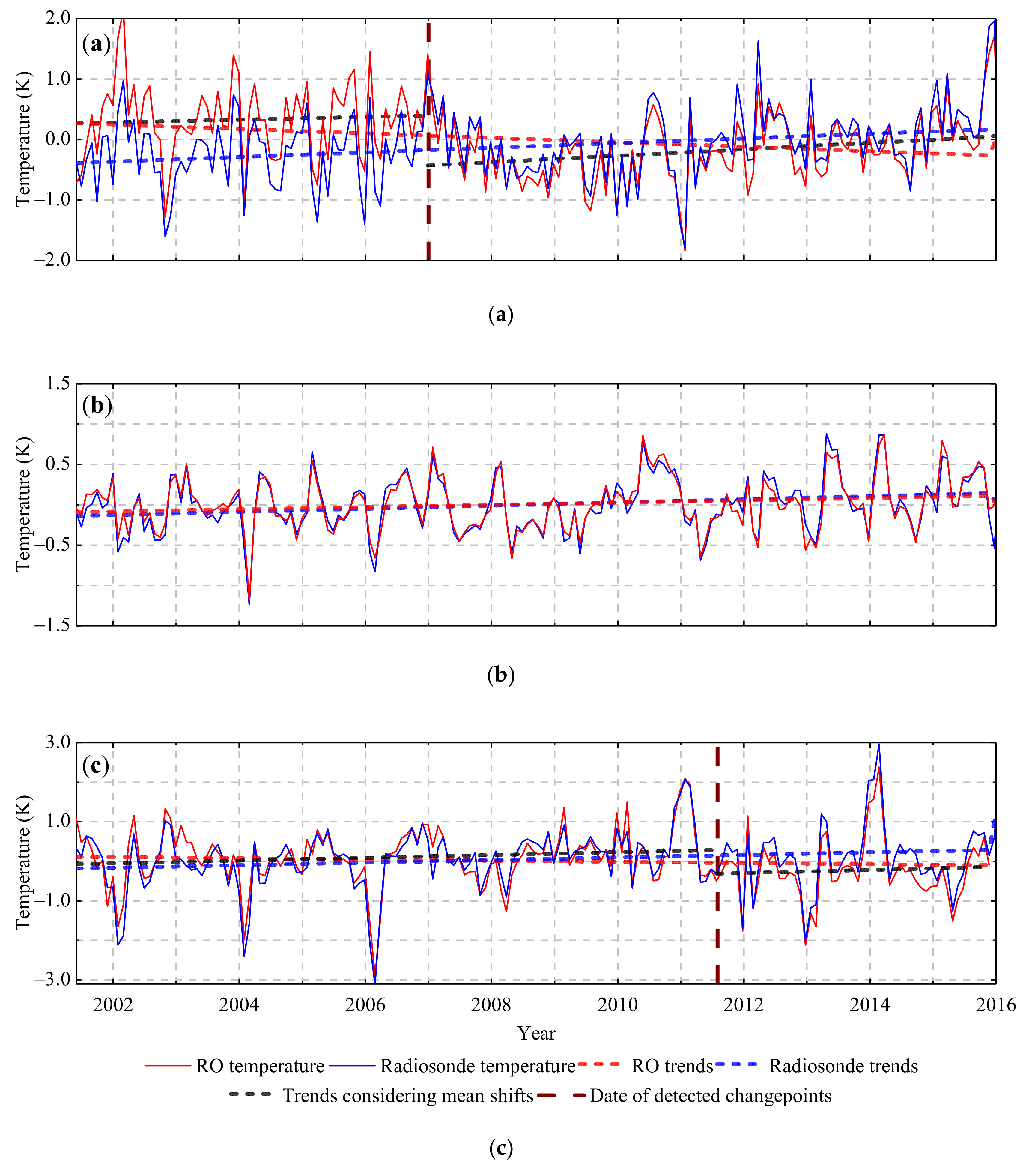
To investigate the influence of the temporal mean shifts on climate studies, we collected data from radiosonde stations located at latitudes of 20°N–60°N: a total of 167 stations. The means of the RO- and radiosonde-based layer-average deseasonalized temperature series at the 167 stations were calculated in the lower troposphere, the UTLS region, and the high-altitude region. The results are shown in Figure 8.
The trends for the atmospheric temperature were obtained from a simple linear regression model that was used to fit the deseasonalized temperature series. The radiosonde- and RO-based temperature trends were 0.38/−0.37 K, 0.20/0.14 K, and 0.32/0.15 K per decade (radiosonde/RO trend) in the lower troposphere, the UTLS region, and the high-altitude region, respectively (the blue and red dotted lines in Figure 8). It should be noted that the two temperature trends were similar in the UTLS region, while in the lower troposphere and the high-altitude region, the linear trend estimates of the RO were negatively biased owing to the existing breakpoints.
Furthermore, we detected the changepoints in the RO layer-average series using the PMTred algorithm, also with the nominal level of confidence of 0.99. One changepoint was detected in the lower troposphere series in December 2006, and another changepoint was detected in the high-altitude region series (in July 2011; shown by the brown dotted lines in Figure 8a,c). Then, a “piecewise line” that allows for mean shifts at the times of the known changepoints was used to fit the temperature series, and segmented RO-based temperature trends were obtained. The segmented RO-based temperature trends show much better agreement with the radiosonde-based trends, with values of 0.23 K/decade (from May 2001 to December 2006) and 0.53 K/decade (January 2007 to December 2015) in the lower troposphere (the black dotted line in Figure 8a) and 0.35 K/decade (from May 2001 to July 2011) and 0.39 K/decade (August 2011 to December 2015) in the high-altitude region (Figure 8c). Note that the trends cannot represent the true state of the atmosphere in the northern middle latitudes, because most of the radiosonde stations are located on the mainland.

5. Conclusions

In this study, taking atmospheric temperature as an example, the systematic discrepancies between the RO profiles collected in different missions were investigated. Then, the homogeneities of the long-term RO temperature climatologies were assessed by comparing them against radiosonde temperature records.
The systematic discrepancies between the temperature profiles from the selected three RO missions were assessed through profile-to-profile comparisons between RO profiles and nearby radiosonde observations and between the co-located profiles from different RO missions. The temperature profiles from the COSMIC and Metop missions were found to be well-matched at most altitude levels with mean differences of 0–0.1 K (Metop COSMIC). The CHAMP temperature profiles showed a good level of consistency with the COSMIC and Metop profiles in the UTLS region, while some warm biases with a maximum value of about 0.5 K were found in the lower troposphere and the high-altitude region, especially in the tropical region.
Through the comparison between the RO- and radiosonde-based climatologies, we found that RO-based climatologies showed high consistency in the UTLS region, while evident temporal mean shifts were observed in the lower troposphere and the high-altitude region. To identify the potential temporal inhomogeneities in the RO-based climatologies, the changepoints in the RO temperature series at the 203 selected stations and 29 altitude levels were detected by the PMTred method using the radiosonde temperature series as a reference. The results obtained for the changepoint detection analysis indicate that the proportion of homogeneous series was smallest in the lower troposphere (61.8%) and largest in the UTLS region (80.1%).
The reasons for the detected temporal inhomogeneities were discussed. First, because the radiosonde-based climatologies were used as the reference data for changepoint detection, the potential temporal inhomogeneity of the radiosonde data, which mainly results from changes in instruments and observation practices used by radiosonde stations, will influence the detection results. Second, the systematic discrepancies between the temperature profiles from different RO missions are reflected in the multi-mission RO-based climatologies. Furthermore, the residual sampling error and the variation in the monthly number of profiles also affect the detected temporal inhomogeneities.
To investigate the influence of temporal mean shifts on the usage of long-term RO climatologies, the trends in the atmospheric temperature were estimated from a linear function fitting of the 15-year deseasonalized temperature records. The radiosonde- and RO-based trends were 0.38/−0.37 K/decade, 0.20/0.14 K/decade, and 0.32/−0.15 K/decade (radiosonde/RO trends) in the lower troposphere, UTLS region, and the high-altitude region, respectively. It was found that the two temperature trends had the best agreement in the UTLS region, while in the lower troposphere and the high-altitude region, the linear trends of the RO temperature records showed a negative bias compared with that of the radiosonde records.
The results from this study demonstrate that the homogeneity of the RO-based climatologies and its agreement with radiosonde are very good in the UTLS region. However, in the lower troposphere and high-altitude region, the development of long-term multi-mission RO-based climatologies still presents many challenges, and factors such as the systematic discrepancies between multi-mission RO data, the residual sampling error, and data numbers should be thoroughly considered.

Author Contributions

Conceptualization, Z.S. and K.Z.; methodology, Z.S. and D.Z.; software, Q.H.; validation, L.L. and D.Z.; formal analysis, Z.S. and M.W.; writing—original draft preparation, Z.S.; writing—review and editing, S.W.; visualization, Z.S.; supervision, K.Z.; project administration, K.Z.; funding acquisition, K.Z. All authors have read and agreed to the published version of the manuscript.

Funding

This work was funded by the State Key Program of the National Natural Science Foundation of China (Grant No. 41730109) and the National Natural Science Foundation of China (Grant No. 41874040).

Institutional Review Board Statement

Not applicable.

Informed Consent Statement

Not applicable.

Data Availability Statement

IGRA-2 radiosonde dataset can be obtained from ftp://ftp.ncdc.noaa.gov/pub/data/igra (accessed on 15 November 2020). CDAAC RO products can be obtained from https://cdaac-www.cosmic.ucar.edu/cdaac/tar/rest.html (accessed on 10 August 2020).

Acknowledgments

We acknowledge CDAAC for the use of the GNSS-RO datasets. We are grateful to NCEI for the IGRA-2 dataset. We also thank ECMWF for providing the short-term forecast. We also thank the two anonymous reviewers for their role in improving the manuscript.

Conflicts of Interest

The authors declare no conflict of interest.

References

  1. Eshleman, V.; Fjeldbo, G. The Atmosphere of Mars Analyzed by Integral Inversion of the Mariner 6 Occultation Data Final Report; NASA: Washington, DC, USA, 1967. [Google Scholar]
  2. Fjeldbo, G.; Eshleman, V.R. Atmosphere of Venus as studied with the Mariner 5 dual radio-frequency occultation experiment. Radio Sci. 1969, 4, 879–897. [Google Scholar] [CrossRef]
  3. Hocke, K. Inversion of GPS meteorology data. Ann. Geophys. 1997, 15, 443–450. [Google Scholar] [CrossRef]
  4. Smith, E.; Weintraub, S. The constants in the equation for atmospheric refractive index at radio frequencies. Proc. IRE 1953, 50, 1035–1037. [Google Scholar] [CrossRef] [Green Version]
  5. Pirscher, B. Multi-Satellite Climatologies of Fundamental Atmospheric Variables from Radio Occulation and Their Validation. Ph.D. Thesis, University of Graz, Graz, Austria, 2010. [Google Scholar]
  6. Gorbunov, M.E.; Kornblueh, L. Analysis and validation of GPS/MET radio occultation data. J. Geophys. Res. Atmos. 2001, 106, 17161–17169. [Google Scholar] [CrossRef]
  7. Reigber, C.; Lühr, H.; Schwintzer, P. CHAMP mission status. Adv. Space Res. 2002, 30, 129–134. [Google Scholar] [CrossRef]
  8. Anthes, R.A.; Bernhardt, P.A.; Chen, Y.; Cucurull, L.; Dymond, K.F.; Ector, D.; Healy, S.B.; Ho, S.P.; Hunt, D.C.; Kuo, Y.H.; et al. The COSMIC/FORMOSAT-3 mission: Early results. Bull. Am. Meteor. Soc. 2008, 89, 313–334. [Google Scholar] [CrossRef]
  9. Schreiner, W.; Sokolovskiy, S.; Hunt, D.; Rocken, C.; Kuo, Y.-H. Analysis of GPS radio occultation data from the FORMOSAT-3/COSMIC and Metop/GRAS missions at CDAAC; 1867–1381. Atmos. Meas. Tech. 2011, 4, 2255–2272. [Google Scholar] [CrossRef] [Green Version]
  10. Scherllin-Pirscher, B.; Steiner, A.K.; Kirchengast, G.; Schwärz, M.; Leroy, S. The power of vertical geolocation of atmospheric profiles from GNSS radio occultation: Power of RO vertical geolocation. J. Geophys. Res. Atmos. 2017, 122, 1595–1616. [Google Scholar] [CrossRef]
  11. Zhou, W.; Yang, S.; Jiang, X.; Guo, Q. Estimating planetary boundary layer height over the Tibetan Plateau using COSMIC radio occultation data. Acta Meteorol. Sin. 2018, 76, 117–133. [Google Scholar]
  12. Rieckh, T.; Anthes, R.; Randel, W.; Ho, S.P.; Foelsche, U. Tropospheric dry layers in the tropical western Pacific: Comparisons of GPS radio occultation with multiple data sets. Atmos. Meas. Tech. 2017, 10, 1093–1110. [Google Scholar] [CrossRef] [Green Version]
  13. Schreiner, W.S.; Weiss, J.P.; Anthes, R.A.; Braun, J.; Chu, V.; Fong, J.; Hunt, D.; Kuo, Y.H.; Meehan, T.; Serafino, W.; et al. COSMIC-2 radio occultation constellation: First results. Geophys. Res. Lett. 2020, 47, e2019GL086841. [Google Scholar] [CrossRef]
  14. Foelsche, U.; Scherllin-Pirscher, B.; Ladstadter, F.; Steiner, A.K.; Kirchengast, G. Refractivity and temperature climate records from multiple radio occultation satellites consistent within 0.05%. Atmos. Meas. Tech. 2011, 4, 2007–2018. [Google Scholar] [CrossRef] [Green Version]
  15. Steiner, A.K.; Hunt, D.; Ho, S.P.; Kirchengast, G.; Mannucci, A.J.; Scherllin-Pirscher, B.; Gleisner, H.; von Engeln, A.; Schmidt, T.; Ao, C.; et al. Quantification of structural uncertainty in climate data records from GPS radio occultation. Atmos. Chem. Phys. 2013, 13, 1469–1484. [Google Scholar] [CrossRef] [Green Version]
  16. Angerer, B.; Ladstadter, F.; Scherllin-Pirscher, B.; Schwärz, M.; Steiner, A.K.; Foelsche, U.; Kirchengast, G. Quality aspects of the Wegener Center multi-satellite GPS radio occultation record OPSv5. 6. Atmos. Meas. Tech. 2017, 10, 4845–4863. [Google Scholar] [CrossRef] [Green Version]
  17. Steiner, A.K.; Ladstadter, F.; Ao, C.O.; Gleisner, H.; Ho, S.-P.; Hunt, D.; Schmidt, T.; Foelsche, U.; Kirchengast, G.; Kuo, Y.-H.; et al. Consistency and structural uncertainty of multi-mission GPS radio occultation records. Atmos. Meas. Tech. 2020, 13, 2547–2575. [Google Scholar] [CrossRef]
  18. Gleisner, H.; Lauritsen, K.B.; Nielsen, J.K.; Syndergaard, S. Evaluation of the 15-year ROM SAF monthly mean GPS radio occultation climate data record. Atmos. Meas. Tech. 2020, 13, 3081–3098. [Google Scholar] [CrossRef]
  19. Steiner, A.K.; Ladstadter, F.; Randel, W.J.; Maycock, A.C.; Fu, Q.; Claud, C.; Gleisner, H.; Haimberger, L.; Ho, S.P.; Keckhut, P.; et al. Observed temperature changes in the troposphere and stratosphere from 1979 to 2018. J. Clim. 2020, 33, 8165–8194. [Google Scholar] [CrossRef]
  20. Zhang, K.; Fu, E.; Silcock, D.; Wang, Y.; Kuleshov, Y. An investigation of atmospheric temperature profiles in the Australian region using collocated GPS radio occultation and radiosonde data. Atmos. Meas. Tech. 2011, 4, 2087–2092. [Google Scholar] [CrossRef] [Green Version]
  21. Kuo, Y.H.; Wee, T.K.; Sokolovskiy, S.; Rocken, C.; Schreiner, W.; Hunt, D.; Anthes, R.A. Inversion and error estimation of GPS radio occultation data. J. Meteorol. Soc. Jpn. 2004, 82, 507–531. [Google Scholar] [CrossRef] [Green Version]
  22. Wickert, J.; Reigber, C.; Beyerle, G.; König, R.; Marquardt, C.; Schmidt, T.; Grunwaldt, L.; Galas, R.; Meehan, T.K.; Melbourne, W.G. Atmosphere sounding by GPS radio occultation: First results from CHAMP. Geophys. Res. Lett. 2001, 28, 3263–3266. [Google Scholar] [CrossRef] [Green Version]
  23. Wickert, J. Comparison of Vertical Refractivity and Temperature Profiles from Champ with Radiosonde Measurements; GeoForschungsZentrum: Potsdam, Germany, 2004. [Google Scholar]
  24. Fong, C.J.; Whiteley, D.; Yang, E.; Cook, K.; Chu, V.; Schreiner, B.; Ector, D.; Wilczynski, P.; Liu, T.Y.; Yen, N. Space and ground segment performance and lessons learned of the FORMOSAT-3/COSMIC mission: Four years in orbit. Atmos. Meas. Tech. 2011, 4, 1115–1132. [Google Scholar] [CrossRef]
  25. Ho, S.P.; Anthes, R.A.; Ao, C.O.; Healy, S.; Horanyi, A.; Hunt, D.; Mannucci, A.J.; Pedatella, N.; Randel, W.J.; Simmons, A.; et al. The COSMIC/FORMOSAT-3 radio occultation mission after 12 Years: Accomplishments, remaining challenges, and potential impacts of COSMIC-2. Bull. Am. Meteor. Soc. 2020, 101, E1107–E1136. [Google Scholar] [CrossRef] [Green Version]
  26. Luntama, J.P.; Kirchengast, G.; Borsche, M.; Foelsche, U.; Steiner, A.; Healy, S.; von Engeln, A.; O’Clerigh, E.; Marquardt, C. Prospects of the Eps Gras mission for operational atmospheric applications. Bull. Am. Meteor. Soc. 2008, 89, 1863–1875. [Google Scholar] [CrossRef] [Green Version]
  27. Gilpin, S.; Rieckh, T.; Anthes, R. Reducing representativeness and sampling errors in radio occultation–radiosonde comparisons. Atmos. Meas. Tech. 2018, 11, 2567–2582. [Google Scholar] [CrossRef] [Green Version]
  28. Nafisi, V.; Urquhart, L.; Santos, M.C.; Nievinski, F.G.; Böhm, J.; Wijaya, D.D.; Schuh, H.; Ardalan, A.A.; Hobiger, T.; Ichikawa, R.; et al. Comparison of ray-tracing packages for troposphere delays. IEEE Trans. Geosci. Remote Sensi. 2012, 50, 469–481. [Google Scholar] [CrossRef]
  29. Borsche, M.; Gobiet, A.; Steiner, A.K.; Foelsche, U.; Kirchengast, G.; Schmidt, T.; Wickert, J. Pre-operational retrieval of radio occultation based climatologies. In Atmosphere and Climate; Foelsche, U., Kirchengast, G., Steiner, A., Eds.; Springer: Berlin/Heidelberg, Germany, 2006; pp. 315–323. [Google Scholar]
  30. Foelsche, U.; Gobiet, A.; Steiner, A.K.; Borsche, M.; Wickert, J.; Schmidt, T.; Kirchengast, G. Global climatologies based on radio occultation data: The CHAMPCLIM project. In Atmosphere and Climate; Foelsche, U., Kirchengast, G., Steiner, A., Eds.; Springer: Berlin/Heidelberg, Germany, 2006; pp. 303–314. [Google Scholar]
  31. Foelsche, U.; Kirchengast, G.; Borsche, M.; Pirscher, B.; Steiner, A. Creating a Consistent Radio Occultation Data Base for Climate Studies in the Upper Troposphere and Lower Stratosphere. In Proceedings of the ECMWF GRAS-SAF Workshop on Applications of RO Measurements, Graz, Austria, 16–18 June 2008; pp. 151–165. [Google Scholar]
  32. Leroy, S.; Ao, C.O.; Verkhoglyadova, O. Mapping GPS radio occultation data by Bayesian interpolation. J. Atmos. Oceanic Technol. 2012, 29, 1062–1074. [Google Scholar] [CrossRef]
  33. Shen, Z.; Zhang, K.; He, Q.; Wan, M.; Li, L.; Wu, S. Quest over the sampling error of COSMIC radio occultation temperature climatologies. J. Atmos. Oceanic Technol. 2021, 38, 441–458. [Google Scholar] [CrossRef]
  34. Berrisford, P.; Dee, D.; Fielding, K.; Fuentes, M.; Kallberg, P.; Kobayashi, S.; Uppala, S. The ERA-Interim Archive; European Centre for Medium-Range Weather Forecasts: Reading, UK, 2009; p. 16. [Google Scholar]
  35. Foelsche, U.; Kirchengast, G.; Steiner, A.K. Global climate monitoring based on CHAMP/GPS radio occultation data. In First CHAMP Mission Results for Gravity, Magnetic and Atmospheric Studies; Reigber, C., Lühr, H., Schwintzer, P., Eds.; Springer: Berlin/Heidelberg, Germany, 2003; pp. 397–407. [Google Scholar]
  36. Pirscher, B.; Foelsche, U.; Lackner, B.; Kirchengast, G. Local time influence in single-satellite radio occultation climatologies from Sun-synchronous and non-Sun-synchronous satellites. J. Geophys. Res. Atmos. 2007, 112, D11119. [Google Scholar] [CrossRef] [Green Version]
  37. Foelsche, U.; Pirscher, B.; Borsche, M.; Steiner, A.K.; Kirchengast, G.; Rocken, C. Climatologies based on radio occultation data from CHAMP and Formosat-3/COSMIC. In New Horizons in Occultation Research: Studies in Atmosphere and Climate; Steiner, A., Pirscher, B., Foelsche, U., Kirchengast, G., Eds.; Springer: Berlin/Heidelberg, Germany, 2009; pp. 181–194. [Google Scholar]
  38. Ladstadter, F.; Steiner, A.K.; Foelsche, U.; Haimberger, L.; Tavolato, C.; Kirchengast, G. An assessment of differences in lower stratospheric temperature records from (A)MSU, radiosondes, and GPS radio occultation. Atmos. Meas. Tech. 2011, 4, 1965–1977. [Google Scholar] [CrossRef] [Green Version]
  39. Wickert, J.; Michalak, G.; Schmidt, T.; Beyerle, G.; Cheng, C.Z.; Healy, S.B.; Heise, S.; Huang, C.Y.; Jakowski, N.; Köhler, W.; et al. GPS radio occultation: Results from CHAMP, GRACE and FORMOSAT-3/COSMIC. Terr. Atmos. Ocean. Sci. 2009, 20, 35–50. [Google Scholar] [CrossRef] [Green Version]
  40. Benzon, H.H. Wave propagation simulation of radio occultations based on ECMWF refractivity profiles. Radio Sci. 2015, 50, 778–788. [Google Scholar] [CrossRef]
  41. Li, Y.; Yuan, Y.; Wang, X. Assessments of the retrieval of atmospheric profiles from GNSS Radio occultation data in moist tropospheric conditions using Radiosonde Data. Remote Sens. 2020, 12, 2717. [Google Scholar] [CrossRef]
  42. Ho, S.; Peng, L.; Vömel, H. Characterization of the long-term radiosonde temperature biases in the upper troposphere and lower stratosphere using COSMIC and Metop-A/GRAS data from 2006 to 2014. Atmos. Chem. Phys. 2017, 17, 4493–4511. [Google Scholar] [CrossRef] [Green Version]
  43. Wang, X.L.; Wen, Q.H.; Wu, Y. Penalized maximalt test for detecting undocumented mean change in climate data series. J. Appl. Meteorol. Climatol. 2007, 46, 916–931. [Google Scholar] [CrossRef]
  44. Wang, X.L. Accounting for autocorrelation in detecting mean shifts in climate data series using the penalized maximal t or F Test. J. Appl. Meteorol. Climatol. 2008, 47, 2423–2444. [Google Scholar] [CrossRef]
  45. Healy, S.B.; Eyre, J.R. Retrieving temperature, water vapour and surface pressure information from refractive-index profiles derived by radio occultation: A simulation study. Quart. J. Royal Meteorol. Soc. 2000, 126, 1661–1683. [Google Scholar] [CrossRef]
  46. Untch, A.; Miller, M.; Hortal, M.; Buizza, R.; Janssen, P. Towards a global meso-scale model: The high resolution system T799L91 and T399L62 EPS. ECMWF Newsl. 2006, 108, 6–13. [Google Scholar]
  47. Gobiet, A.; Kirchengast, G. Advancements of global navigation satellite system radio occultation retrieval in the upper stratosphere for optimal climate monitoring utility. J. Geophys. Res. 2004, 109. [Google Scholar] [CrossRef] [Green Version]
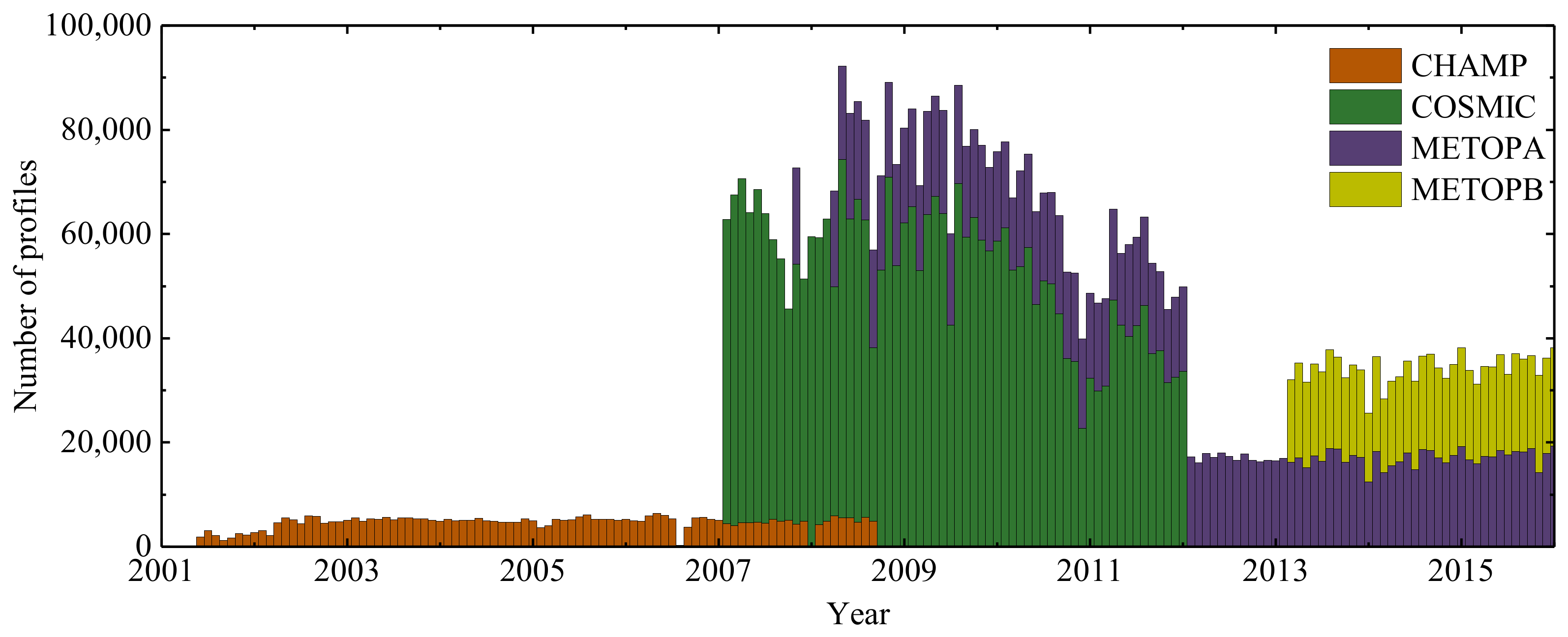
Figure 1. Monthly numbers of radio occultation (RO) atmospheric profiles collecting during a 15-year period from May 2001 to December 2015 from each of the three RO missions.
Remotesensing 13 02278 g001
Figure 2. Geolocations of the 203 selected radiosonde stations used in this study.
Remotesensing 13 02278 g002
Figure 3. (a) Means (solid lines) and standard deviations (dotted lines) of the differences between temperature profiles from RO and nearby radiosonde stations (RO−radiosonde); (b) proportions of available collocation profiles at various altitudes.
Remotesensing 13 02278 g003
Figure 4. Means (solid lines) and standard deviations (dotted lines) of the differences between co-located temperature profiles from different RO missions at latitudinal bands of 90°S–90°N (a), 60°N–90°N (b), 20°N–60°N (c), 20°S–20°N (d), 60°S–20°S (e), and 90°S–60°S (f). The proportions of the co-located RO profiles that penetrate different altitudes are presented in the right panel of each figure.
Remotesensing 13 02278 g004aRemotesensing 13 02278 g004b
Figure 5. Time−altitude structure of the radiosonde-based deseasonalized temperature at (a) Hamamatsu AB and (b) Brownsville/INT; RO-based deseasonalized temperature at (c) Hamamatsu AB and (d) Brownsville/INT; differences between the RO- and radiosonde-based deseasonalized temperatures at (e) Hamamatsu AB and (f) Brownsville/INT, unit K.
Remotesensing 13 02278 g005aRemotesensing 13 02278 g005b
Figure 6. Time−altitude structure of the (a) radiosonde-based and (b) RO-based mean temperature climatologies at the 203 stations; (c) the differences between the RO- and radiosonde-based mean temperature climatologies; time series of the RO- and radiosonde-based mean layer-average deseasonalized temperature at the 203 stations (red and blue solid lines) in (d) the lower troposphere, (e) the UTLS, and (f) the high-altitude region (units = K). The vertical dashed lines represent the dates of the observed temporal mean shifts.
Remotesensing 13 02278 g006aRemotesensing 13 02278 g006b
Figure 7. (a,b) Monthly numbers of detected change points in the reference and tested fields (radiosonde- and RO-based temperature climatologies) at the 203 stations and 29 altitude levels from May 2001 to December 2015; (c) monthly number of detected changepoints in the RO-based temperature climatologies using the radiosonde temperature field as the reference.
Remotesensing 13 02278 g007
Figure 8. Means of the layer-average deseasonalized temperature time series of the 167 RO- and radiosonde-based temperature stations in (a) the lower troposphere, (b) the UTLS region, and (c) the high-altitude region (units = K).
Remotesensing 13 02278 g008
Table 1. Information about the valid co-located radio occultation (RO) profiles.
MissionsPeriod for comparisonNumber of Co-Located Profiles
CHAMP – COSMIC1 June 2007–
26 August 2008
28,026
Metop-A – COSMIC1 October 2007–
31 December 2011
220,362
Metop-A – Metop-B1 October 2007–
31 December 2011
100,852
Table 2. Means and standard deviations of the differences between co-located temperature profiles from different RO missions at altitudes of 4, 14, and 26 km in the same six latitude regions as shown in Figure 4.
Latitude RangeAltitude
[km]
Mean Temperature Differences (Standard Deviation) [K]
CHAMP – COSMICMETOPA – COSMICMETOPA – METOPB
90°S–90°N40.23 (2.00)0.09 (2.38)0.01 (2.36)
140.06 (1.42)0.00 (1.55)0.00 (1.63)
260.14 (1.79)0.04 (1.86)−0.01 (1.77)
60°N–90°N40.05 (1.96)0.03 (2.40)0.00 (2.50)
140.03 (1.36)0.02 (1.39)0.00 (1.60)
260.01 (1.85)0.04 (1.86)−0.01 (1.72)
20°N–60°N40.31 (2.02)0.11 (2.36)0.04 (2.31)
140.07 (1.49)0.00 (1.58)0.02 (1.66)
260.21 (1.65)0.04 (1.78)0.00 (1.74)
20°S–20°N40.56 (1.18)0.08 (1.38)0.00 (1.48)
140.11 (0.91)0.05 (0.96)−0.01 (1.08)
260.29 (1.71)0.09 (1.74)0.01 (1.75)
60°S–20°S40.25 (2.20)0.11 (2.57)−0.01 (2.53)
140.05 (1.59)0.01 (1.69)−0.01 (1.72)
260.20 (1.84)0.05 (1.92)−0.02 (1.77)
90°S–60°S40.08 (2.04)0.08 (2.42)−0.01 (2.50)
140.06 (1.41)−0.05 (1.65)0.00 (1.78)
26−0.06 (1.85)0.00 (1.99)−0.02 (1.92)
Table 3. Number of deseasonalized RO temperature series that contain zero, one, two, and three or more mean shifts. The percentage in each bracket is the proportion of the series containing N mean shifts of the total number of series in different altitude ranges.
Altitude RangesNumber of Series Containing N Mean ShiftsTotal
N = 0N = 1N = 2 N ≥ 3
Lower troposphere879 (61.8%)464 (32.7%)41 (2.9%)37 (2.6%)1421
UTLS region1950 (80.1%)397 (16.3%)67 (2.8%)22 (1.0%)2436
High-altitude region1496 (73.7%)457 (22.5%)51 (2.5%)26 (1.3%)2030
Total4325 (73.5%)1318 (22.4%)159 (2.7%)85 (1.4%)5887
Publisher’s Note: MDPI stays neutral with regard to jurisdictional claims in published maps and institutional affiliations.