
Comparative Analysis of Two Machine Learning Algorithms in Predicting Site-Level Net Ecosystem Exchange in Major Biomes

 ,
,  ,
, 

Abstract
1. Introduction
2. Data and Methods
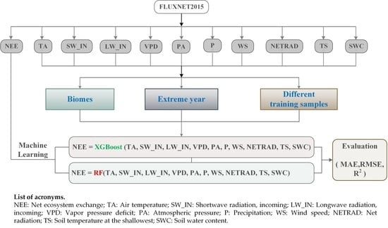
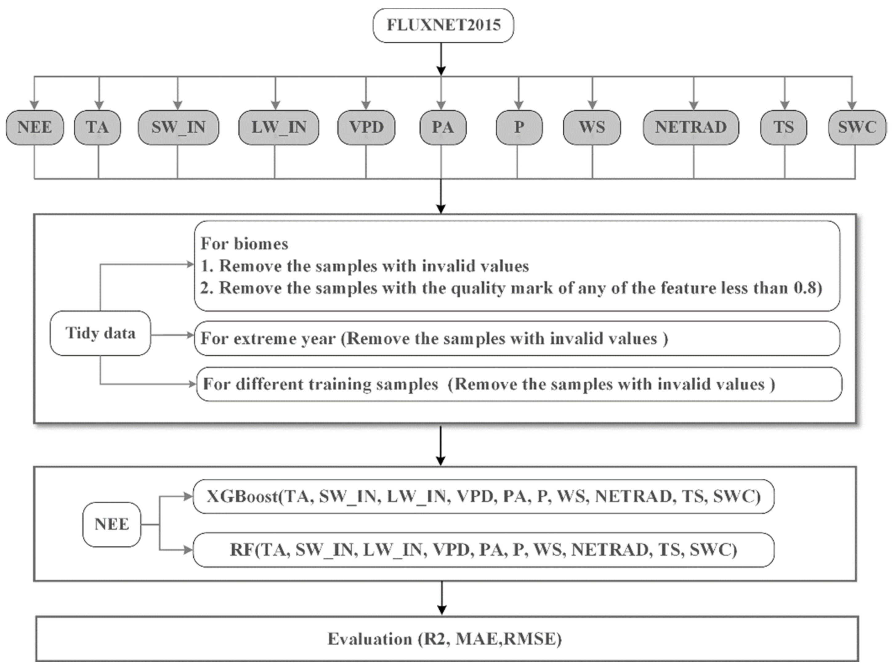
2.1. Data Sources
2.2. Machine Learning Algorithms
2.2.1. Random Forest
2.2.2. XGBoost
2.3. Model Development
2.3.1. Biome-level Simulation
2.3.2. Simulations under Extreme Climate Conditions
2.3.3. Sample Size Sufficiency for Model Estimation
2.4. Bernaola-Galvan Segmentation Algorithm
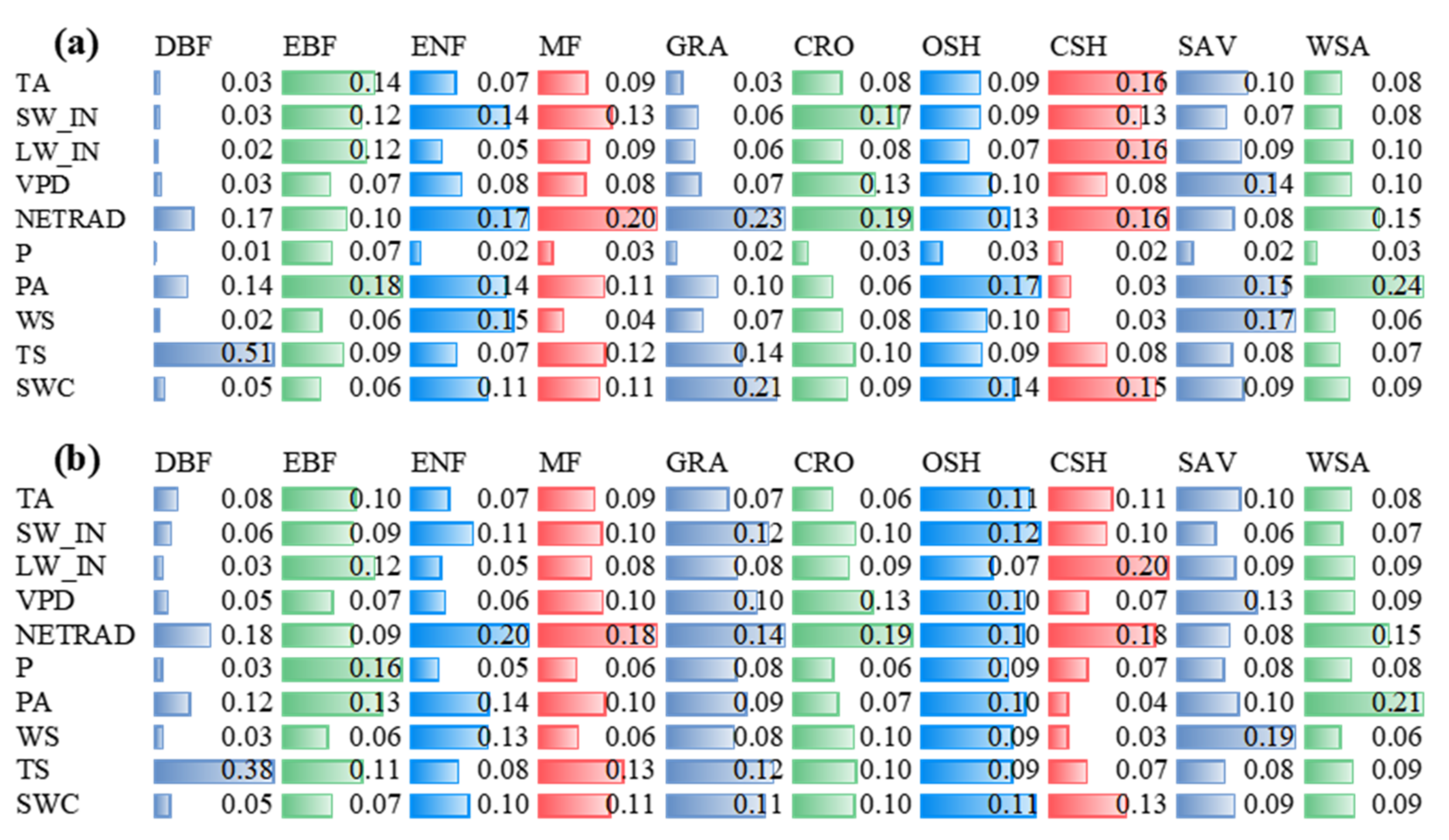
2.5. Feature Analysis
3. Results
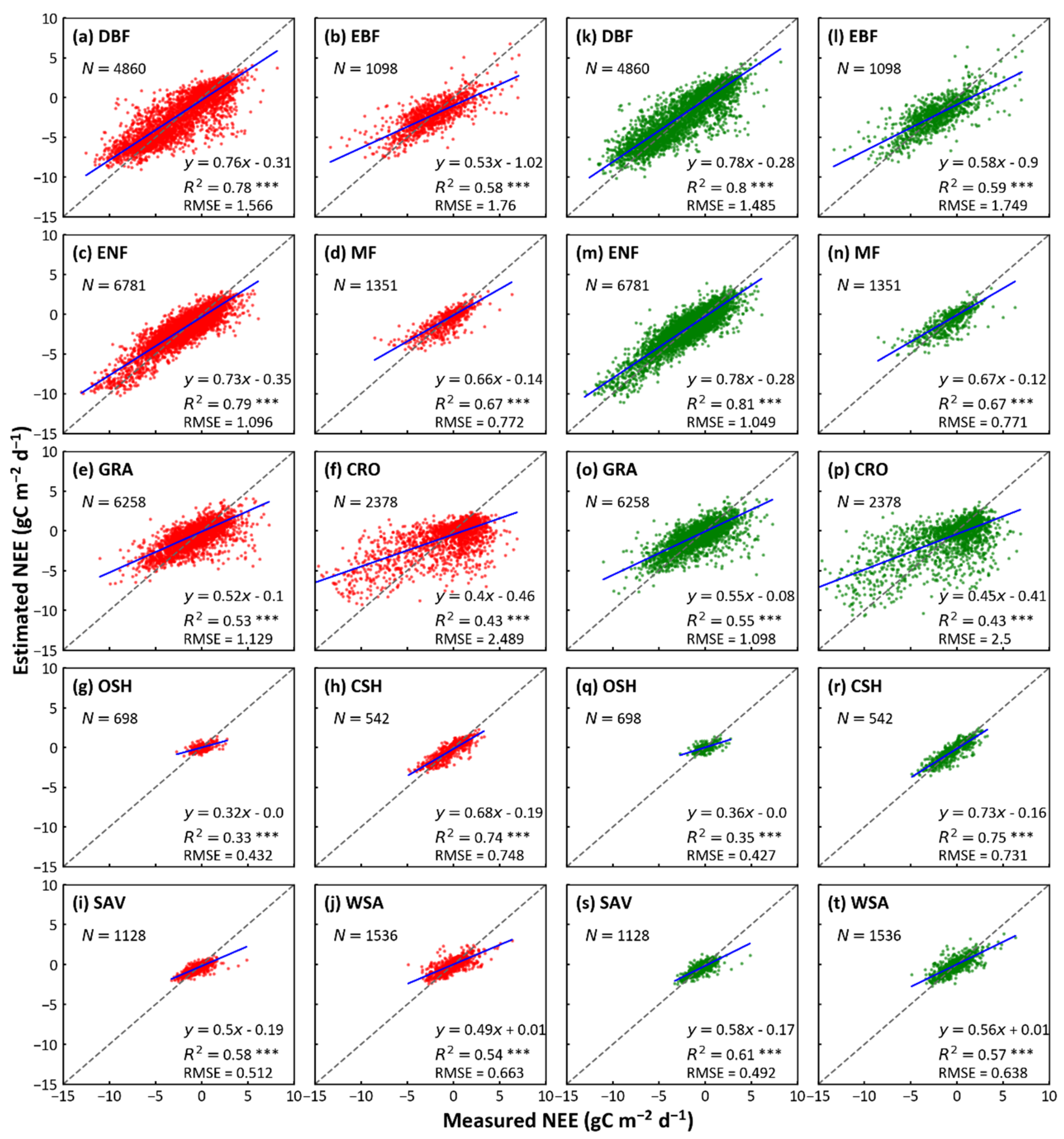
3.1. Biome-Level Model Performance
3.2. Environmental Conditions
3.3. Model Performance in Simulating NEE under Extreme Climate Conditions
3.4. Model Performance in Simulating NEE under Extreme Climate Conditions
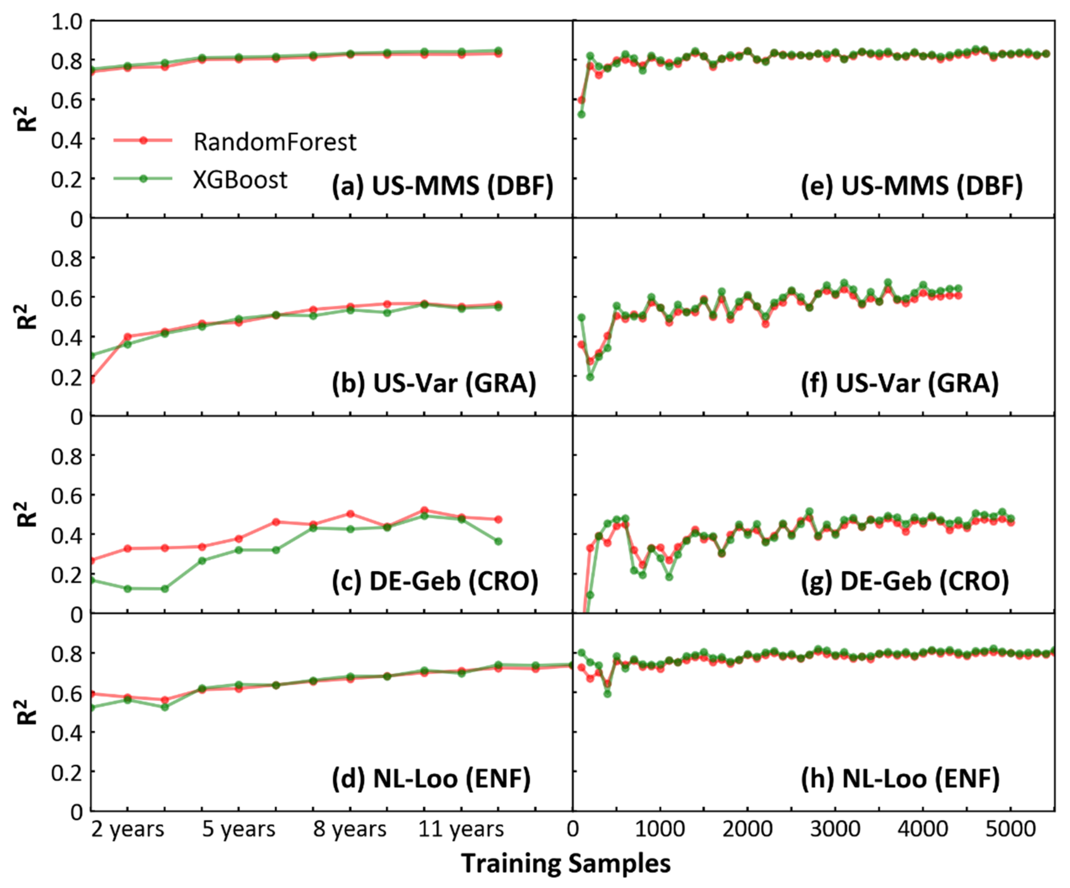
3.5. Quantitative Analysis of Sample Size in Reaching Feasible Model Performance
4. Discussion
4.1. Quantitative Analysis of Sample Size in Reaching Feasible Model Performance
4.2. Environmental Controls as Estimated by Two ML Algorithms
4.3. Effects of Extreme Climatic Conditions on NEE Prediction at Biome Level
4.4. Effects of Extreme Climatic Conditions on NEE Prediction at Biome Level
5. Conclusions
Supplementary Materials
Author Contributions
Funding
Institutional Review Board Statement
Informed Consent Statement
Data Availability Statement
Acknowledgments
Conflicts of Interest
References
- Post, W.M.; Peng, T.-H.; Emanuel, W.R.; King, A.W.; Dale, V.H.; DeAngelis, D.L. The global carbon cycle. Am. Sci. 1990, 78, 310–326. [Google Scholar]
- Friend, A.D.; Arneth, A.; Kiang, N.Y.; Lomas, M.; Ogee, J.; Rödenbeck, C.; Running, S.W.; Santaren, J.D.; Sitch, S.; Viovy, N. FLUXNET and modelling the global carbon cycle. Glob. Chang. Biol. 2007, 13, 610–633. [Google Scholar] [CrossRef]
- Isson, T.T.; Planavsky, N.J.; Coogan, L.A.; Stewart, E.M.; Ague, J.J.; Bolton, E.W.; Zhang, S.; McKenzie, N.R.; Kump, L.R. Evolution of the global carbon cycle and climate regulation on Earth. Glob. Biogeochem. Cycles 2020, 34, e2018GB006061. [Google Scholar] [CrossRef]
- Chapin, F.S.; Woodwell, G.M.; Randerson, J.T.; Rastetter, E.B.; Lovett, G.M.; Baldocchi, D.D.; Clark, D.A.; Harmon, M.E.; Schimel, D.S.; Valentini, R.; et al. Reconciling Carbon-cycle Concepts, Terminology, and Methods. Ecosystems 2006, 9, 1041–1050. [Google Scholar] [CrossRef]
- Baldocchi, D.D. Assessing the eddy covariance technique for evaluating carbon dioxide exchange rates of ecosystems: Past, present and future. Glob. Chang. Biol. 2003, 9, 479–492. [Google Scholar] [CrossRef]
- Pastorello, G.; Trotta, C.; Canfora, E.; Chu, H.; Christianson, D.; Cheah, Y.W.; Poindexter, C.; Chen, J.; Elbashandy, A.; Humphrey, M.; et al. The FLUXNET2015 dataset and the ONEFlux processing pipeline for eddy covariance data. Sci. Data 2020, 7, 225. [Google Scholar] [CrossRef] [PubMed]
- Baldocchi, D.D.; Hincks, B.B.; Meyers, T.P. Measuring Biosphere-Atmosphere Exchanges of Biologically Related Gases with Micrometeorological Methods. Ecology 1988, 69, 1331–1340. [Google Scholar] [CrossRef]
- Baldocchi, D.; Falge, E.; Gu, L.H.; Olson, R.; Hollinger, D.; Running, S.; Anthoni, P.; Bernhofer, C.; Davis, K.; Evans, R.; et al. FLUXNET: A new tool to study the temporal and spatial variability of ecosystem-scale carbon dioxide, water vapor, and energy flux densities. Bull. Am. Meteorol. Soc. 2001, 82, 2415–2434. [Google Scholar] [CrossRef]
- Sitch, S.; Smith, B.; Prentice, I.C.; Arneth, A.; Bondeau, A.; Cramer, W.; Kaplan, J.O.; Levis, S.; Lucht, W.; Sykes, M.T.; et al. Evaluation of ecosystem dynamics, plant geography and terrestrial carbon cycling in the LPJ dynamic global vegetation model. Glob. Chang. Biol. 2003, 9, 161–185. [Google Scholar] [CrossRef]
- Krinner, G.; Viovy, N.; de Noblet-Ducoudre, N.; Ogee, J.; Polcher, J.; Friedlingstein, P.; Ciais, P.; Sitch, S.; Prentice, I.C. A dynamic global vegetation model for studies of the coupled atmosphere-biosphere system. Glob. Biogeochem. Cycles 2005, 19. [Google Scholar] [CrossRef]
- Lawrence, D.M.; Oleson, K.W.; Flanner, M.G.; Thornton, P.E.; Swenson, S.C.; Lawrence, P.J.; Zeng, X.B.; Yang, Z.L.; Levis, S.; Sakaguchi, K.; et al. Parameterization Improvements and Functional and Structural Advances in Version 4 of the Community Land Model. J. Adv. Model. Earth Syst. 2011, 3. [Google Scholar] [CrossRef]
- Xu, X.; Elias, D.A.; Graham, D.E.; Phelps, T.J.; Carroll, S.L.; Wullschleger, S.D.; Thornton, P.E. A microbial functional group-based module for simulating methane production and consumption: Application to an incubated permafrost soil. J. Geophys. Res. Biogeosci. 2015, 120, 1315–1333. [Google Scholar] [CrossRef]
- Wang, Y.; Yuan, F.; Yuan, F.; Gu, B.; Hahn, M.S.; Torn, M.S.; Ricciuto, D.M.; Kumar, J.; He, L.; Zona, D.; et al. Mechanistic Modeling of Microtopographic Impacts on CO2 and CH4 Fluxes in an Alaskan Tundra Ecosystem Using the CLM-Microbe Model. J. Adv. Model. Earth Syst. 2019, 11, 4288–4304. [Google Scholar] [CrossRef]
- Jung, M.; Schwalm, C.; Migliavacca, M.; Walther, S.; Reichstein, M. Scaling carbon fluxes from eddy covariance sites to globe: Synthesis and evaluation of the FLUXCOM approach. Biogeosciences 2020, 17, 1343–1365. [Google Scholar] [CrossRef]
- Zeng, J.; Matsunaga, T.; Tan, Z.H.; Saigusa, N.; Shirai, T.; Tang, Y.; Peng, S.; Fukuda, Y. Global terrestrial carbon fluxes of 1999–2019 estimated by upscaling eddy covariance data with a random forest. Sci. Data 2020, 7, 313. [Google Scholar] [CrossRef] [PubMed]
- Tian, H.; Xu, X.; Lu, C.; Liu, M.; Ren, W.; Chen, G.; Melillo, J.; Liu, J. Net exchanges of CO2, CH4, and N2O between China’s terrestrial ecosystems and the atmosphere and their contributions to global climate warming. J. Geophys. Res. Biogeosci. 2011, 116. [Google Scholar] [CrossRef]
- Tian, H.; Chen, G.; Zhang, C.; Liu, M.; Sun, G.; Chappelka, A.; Ren, W.; Xu, X.; Lu, C.; Pan, S.; et al. Century-Scale Responses of Ecosystem Carbon Storage and Flux to Multiple Environmental Changes in the Southern United States. Ecosystems 2012, 15, 674–694. [Google Scholar] [CrossRef]
- Song, X.; Tian, H.Q.; Xu, X.F.; Hui, D.F.; Chen, G.S.; Sommers, G.; Marzen, L.; Liu, M.L. Projecting terrestrial carbon sequestration of the southeastern United States in the 21st century. Ecosphere 2013, 4, 18. [Google Scholar] [CrossRef]
- Li, X.; Hu, X.-M.; Cai, C.; Jia, Q.; Zhang, Y.; Liu, J.; Xue, M.; Xu, J.; Wen, R.; Crowell, S.M.R. Terrestrial CO2 Fluxes, Concentrations, Sources and Budget in Northeast China: Observational and Modeling Studies. J. Geophys. Res. Atmos. 2020, 125. [Google Scholar] [CrossRef]
- Sefrin, O.; Riese, F.M.; Keller, S. Deep Learning for Land Cover Change Detection. Remote Sens. 2021, 13, 78. [Google Scholar] [CrossRef]
- Kianian, B.; Liu, Y.; Chang, H.H. Imputing Satellite-Derived Aerosol Optical Depth Using a Multi-Resolution Spatial Model and Random Forest for PM2.5 Prediction. Remote Sens. 2021, 13, 126. [Google Scholar] [CrossRef]
- Xiao, J.; Ollinger, S.V.; Frolking, S.; Hurtt, G.C.; Hollinger, D.Y.; Davis, K.J.; Pan, Y.; Zhang, X.; Deng, F.; Chen, J.; et al. Data-driven diagnostics of terrestrial carbon dynamics over North America. Agric. For. Meteorol. 2014, 197, 142–157. [Google Scholar] [CrossRef]
- Zhang, J.X.; Liu, K.; Wang, M. Downscaling Groundwater Storage Data in China to a 1-km Resolution Using Machine Learning Methods. Remote Sens. 2021, 13, 523. [Google Scholar] [CrossRef]
- Kim, Y.; Johnson, M.S.; Knox, S.H.; Black, T.A.; Dalmagro, H.J.; Kang, M.; Kim, J.; Baldocchi, D. Gap-filling approaches for eddy covariance methane fluxes: A comparison of three machine learning algorithms and a traditional method with principal component analysis. Glob. Chang. Biol. 2020, 26, 1499–1518. [Google Scholar] [CrossRef]
- Jordan, M.I.; Mitchell, T.M. Machine learning: Trends, perspectives, and prospects. Science 2015, 349, 255. [Google Scholar] [CrossRef]
- Arel, I.; Rose, D.C.; Karnowski, T.P. Deep Machine Learning-A New Frontier in Artificial Intelligence Research [Research Frontier]. IEEE Comput. Intell. Mag. 2010, 5, 13–18. [Google Scholar] [CrossRef]
- Feng, Q.Y.; Vasile, R.; Segond, M.; Gozolchiani, A.; Wang, Y.; Abel, M.; Havlin, S.; Bunde, A.; Dijkstra, H.A. ClimateLearn: A machine-learning approach for climate prediction using network measures. Geosci. Model. Dev. Discuss. 2016, 2016, 1–18. [Google Scholar] [CrossRef]
- Quade, M.; Gout, J.; Abel, M. Glyph: Symbolic Regression Tools. J. Open Res. Softw. 2019, 7. [Google Scholar] [CrossRef]
- Van Wijk, M.T.; Bouten, W. Water and carbon fluxes above European coniferous forests modelled with artificial neural networks. Ecol. Model. 1999, 120, 181–197. [Google Scholar] [CrossRef]
- Melesse, A.M.; Hanley, R.S. Artificial neural network application for multi-ecosystem carbon flux simulation. Ecol. Model. 2005, 189, 305–314. [Google Scholar] [CrossRef]
- He, H.; Yu, G.; Zhang, L.; Sun, X.; Su, W. Simulating CO2 flux of three different ecosystems in ChinaFLUX based on artificial neural networks. Sci. China Ser. D Earth Sci. 2006, 49, 252–261. [Google Scholar] [CrossRef]
- Kondo, M.; Ichii, K.; Takagi, H.; Sasakawa, M. Comparison of the data-driven top-down and bottom-up global terrestrial CO2exchanges: GOSAT CO2inversion and empirical eddy flux upscaling. J. Geophys. Res. Biogeosci. 2015, 120, 1226–1245. [Google Scholar] [CrossRef]
- Ichii, K.; Ueyama, M.; Kondo, M.; Saigusa, N.; Kim, J.; Carmelita Alberto, M.; Ardoe, J.; Euskirchen, E.S.; Kang, M.; Hirano, T.; et al. New data-driven estimation of terrestrial CO2 fluxes in Asia using a standardized database of eddy covariance measurements, remote sensing data, and support vector regression. J. Geophys. Res. Biogeosci. 2017, 122, 767–795. [Google Scholar] [CrossRef]
- Cortes, C.; Vapnik, V. Support-Vector Networks. Mach. Learn. 1995, 20, 273–297. [Google Scholar] [CrossRef]
- Xiao, J.; Zhuang, Q.; Baldocchi, D.D.; Law, B.E. Estimation of net ecosystem carbon exchange for the conterminous United States by combining MODIS and AmeriFlux data. Agric. For. Meteorol. 2008, 148, 1827–1847. [Google Scholar] [CrossRef]
- Jung, M.; Reichstein, M.; Margolis, H.A.; Cescatti, A.; Richardson, A.D.; Arain, M.A.; Arneth, A.; Bernhofer, C.; Bonal, D.; Chen, J.; et al. Global patterns of land-atmosphere fluxes of carbon dioxide, latent heat, and sensible heat derived from eddy covariance, satellite, and meteorological observations. J. Geophys. Res. Biogeosci. 2011, 116. [Google Scholar] [CrossRef]
- Cai, J.; Xu, K.; Zhu, Y.; Hu, F.; Li, L. Prediction and analysis of net ecosystem carbon exchange based on gradient boosting regression and random forest. Appl. Energy 2020, 262. [Google Scholar] [CrossRef]
- Tramontana, G.; Jung, M.; Schwalm, C.R.; Ichii, K.; Camps-Valls, G.; Ráduly, B.; Reichstein, M.; Arain, M.A.; Cescatti, A.; Kiely, G.; et al. Predicting carbon dioxide and energy fluxes across global FLUXNET sites with regression algorithms. Biogeosciences 2016, 13, 4291–4313. [Google Scholar] [CrossRef]
- Dou, X.; Yang, Y. Estimating forest carbon fluxes using four different data-driven techniques based on long-term eddy covariance measurements: Model comparison and evaluation. Sci. Total Environ. 2018, 627, 78–94. [Google Scholar] [CrossRef]
- Tu, J.V. Advantages and disadvantages of using artificial neural networks versus logistic regression for predicting medical outcomes. J. Clin. Epidemiol. 1996, 49, 1225–1231. [Google Scholar] [CrossRef]
- Gholami, R.; Fakhari, N. Support Vector Machine: Principles, Parameters, and Applications. In Handbook of Neural Computation; Samui, P., Sekhar, S., Balas, V.E., Eds.; Academic Press: Cambridge, UK, 2017; Chapter 27; pp. 515–535. [Google Scholar]
- Kaja, N.; Shaout, A.; Ma, D. An intelligent intrusion detection system. Appl. Intell. 2019, 49, 3235–3247. [Google Scholar] [CrossRef]
- Chen, T.; Guestrin, C. Xgboost: A scalable tree boosting system. In Proceedings of the 22nd Acm Sigkdd International Conference on Knowledge Discovery and Data Mining, San Francisco, CA, USA, 13–17 August 2016; pp. 785–794. [Google Scholar]
- Breiman, L. Random forests. Mach. Learn. 2001, 45, 5–32. [Google Scholar] [CrossRef]
- Pranckevičius, T.; Marcinkevičius, V. Comparison of Naive Bayes, Random Forest, Decision Tree, Support Vector Machines, and Logistic Regression Classifiers for Text Reviews Classification. Balt. J. Mod. Comput. 2017, 5. [Google Scholar] [CrossRef]
- Friedman, J.H. Greedy function approximation: A gradient boosting machine. Ann. Stat. 2001, 29, 1189–1232. [Google Scholar] [CrossRef]
- Breiman, L.; Friedman, J.; Stone, C.J.; Olshen, R.A. Classification and Regression Trees; CRC Press: New York, NY, USA, 1984; pp. 342–346. [Google Scholar]
- Bernaola-Galván, P.; Ivanov, P.C.; Amaral, L.A.N.; Stanley, H.E. Scale invariance in the nonstationarity of human heart rate. Phys. Rev. Lett. 2001, 87, 168105. [Google Scholar] [CrossRef] [PubMed]
- Wang, F.; Wang, Z.M.; Yang, H.B.; Zhao, Y. Study of the temporal and spatial patterns of drought in the Yellow River basin based on SPEI. Sci. China Earth Sci. 2018, 61, 1098–1111. [Google Scholar] [CrossRef]
- Liu, X.; Zhang, Y.; Liu, Y.; Zhao, X.; Zhang, J.; Rui, Y. Characteristics of temperature evolution from 1960 to 2015 in the Three Rivers’ Headstream Region, Qinghai, China. Sci. Rep. 2020, 10, 20272. [Google Scholar] [CrossRef]
- Teklemariam, T.A.; Lafleur, P.M.; Moore, T.R.; Roulet, N.T.; Humphreys, E.R. The direct and indirect effects of inter-annual meteorological variability on ecosystem carbon dioxide exchange at a temperate ombrotrophic bog. Agric. For. Meteorol. 2010, 150, 1402–1411. [Google Scholar] [CrossRef]
- Liu, Y.; Zhou, G.; Du, H.; Berninger, F.; Mao, F.; Li, X.; Chen, L.; Cui, L.; Li, Y.; Zhu, D.; et al. Response of carbon uptake to abiotic and biotic drivers in an intensively managed Lei bamboo forest. J. Environ. Manag. 2018, 223, 713–722. [Google Scholar] [CrossRef]
- Jongen, M.; Pereira, J.S.; Aires, L.M.I.; Pio, C.A. The effects of drought and timing of precipitation on the inter-annual variation in ecosystem-atmosphere exchange in a Mediterranean grassland. Agric. For. Meteorol. 2011, 151, 595–606. [Google Scholar] [CrossRef]
- Reichstein, M.; Bahn, M.; Ciais, P.; Frank, D.; Mahecha, M.D.; Seneviratne, S.I.; Zscheischler, J.; Beer, C.; Buchmann, N.; Frank, D.C.; et al. Climate extremes and the carbon cycle. Nature 2013, 500, 287–295. [Google Scholar] [CrossRef] [PubMed]


| Abbreviation | Long Name | Units |
|---|---|---|
| TA | Air temperature | deg C |
| SW_IN | Shortwave radiation, incoming | W m−2 |
| LW_IN | Longwave radiation, incoming | W m−2 |
| VPD | Vapor pressure deficit | hPa |
| PA | Atmospheric pressure | kPa |
| P | Precipitation | mm d−1 |
| WS | Wind speed | m s−1 |
| NETRAD | Net radiation | W m−2 |
| TS | Soil temperature at the shallowest | deg C |
| SWC | Soil water content at the shallowest | % |
| ID | Site_ID | Site Name | Data Start | Data End | Biome | Sample Size |
|---|---|---|---|---|---|---|
| 1 | AU-ASM | Alice Springs | 2010 | 2014 | SAV | 1418 |
| 2 | AU-Cpr | Calperum | 2010 | 2014 | SAV | 870 |
| 3 | AU-Dry | Dry River | 2008 | 2014 | SAV | 1118 |
| 4 | AU-Emr | Emerald | 2011 | 2013 | GRA | 805 |
| 5 | AU-Gin | Gingin | 2011 | 2014 | WSA | 917 |
| 6 | AU-GWW | Great Western Woodlands, Western Australia, Australia | 2013 | 2014 | SAV | 353 |
| 7 | AU-Lox | Loxton | 2008 | 2009 | DBF | 275 |
| 8 | AU-RDF | Red Dirt Melon Farm, Northern Territory | 2011 | 2013 | WSA | 553 |
| 9 | AU-Rig | Riggs Creek | 2011 | 2014 | GRA | 997 |
| 10 | AU-Rob | Robson Creek, Queensland, Australia | 2014 | 2014 | EBF | 309 |
| 11 | AU-TTE | Ti Tree East | 2012 | 2014 | GRA | 844 |
| 12 | AU-Tum | Tumbarumba | 2001 | 2014 | EBF | 1656 |
| 13 | AU-Wac | Wallaby Creek | 2005 | 2008 | EBF | 295 |
| 14 | AU-Wom | Wombat | 2010 | 2014 | EBF | 912 |
| 15 | AU-Ync | Jaxa | 2012 | 2014 | GRA | 526 |
| 16 | BE-Lon | Lonzee | 2004 | 2014 | CRO | 1713 |
| 17 | BR-Sa3 | Santarem-Km83-Logged Forest | 2000 | 2004 | EBF | 486 |
| 18 | CA-Gro | Ontario-Groundhog River, Boreal Mixedwood Forest | 2003 | 2014 | MF | 2005 |
| 19 | CA-Qfo | Quebec-Eastern Boreal, Mature Black Spruce | 2003 | 2010 | ENF | 2098 |
| 20 | CA-SF1 | Saskatchewan-Western Boreal, forest burned in 1977 | 2003 | 2006 | ENF | 536 |
| 21 | CA-SF3 | Saskatchewan-Western Boreal, forest burned in 1998 | 2001 | 2006 | OSH | 448 |
| 22 | CA-TP4 | Ontario-Turkey Point 1939 Plantation White Pine | 2002 | 2014 | ENF | 2166 |
| 23 | CH-Cha | Chamau | 2005 | 2014 | GRA | 1279 |
| 24 | CH-Dav | Davos | 1997 | 2014 | ENF | 1560 |
| 25 | CN-Cha | Changbaishan | 2003 | 2005 | MF | 789 |
| 26 | CN-Cng | Changling | 2007 | 2010 | GRA | 1002 |
| 27 | CN-Qia | Qianyanzhou | 2003 | 2005 | ENF | 948 |
| 28 | CZ-BK1 | Bily Kriz forest | 2004 | 2014 | ENF | 968 |
| 29 | CZ-BK2 | Bily Kriz grassland | 2004 | 2012 | GRA | 173 |
| 30 | DE-Geb | Gebesee | 2001 | 2014 | CRO | 4555 |
| 31 | DE-Gri | Grillenburg | 2004 | 2014 | GRA | 1931 |
| 32 | DE-Hai | Hainich | 2000 | 2012 | DBF | 3053 |
| 33 | DE-Obe | Oberbärenburg | 2008 | 2014 | ENF | 1449 |
| 34 | DK-Sor | Soroe | 1996 | 2014 | DBF | 188 |
| 35 | FI-Hyy | Hyytiala | 1996 | 2014 | ENF | 322 |
| 36 | FR-LBr | Le Bray | 1996 | 2008 | ENF | 1373 |
| 37 | IT-CA1 | Castel d’Asso1 | 2011 | 2014 | DBF | 221 |
| 38 | IT-CA2 | Castel d’Asso2 | 2011 | 2014 | CRO | 115 |
| 39 | IT-CA3 | Castel d’Asso3 | 2011 | 2014 | DBF | 346 |
| 40 | IT-Isp | Ispra ABC-IS | 2013 | 2014 | DBF | 575 |
| 41 | IT-Lav | Lavarone | 2003 | 2014 | ENF | 1642 |
| 42 | IT-MBo | Monte Bondone | 2003 | 2013 | GRA | 2605 |
| 43 | IT-Noe | Arca di Noe-Le Prigionette | 2004 | 2014 | CSH | 1806 |
| 44 | IT-Ro1 | Roccarespampani 1 | 2000 | 2008 | DBF | 268 |
| 45 | IT-SR2 | San Rossore 2 | 2013 | 2014 | ENF | 580 |
| 46 | IT-Tor | Torgnon | 2008 | 2014 | GRA | 601 |
| 47 | NL-Loo | Loobos | 1996 | 2014 | ENF | 3811 |
| 48 | US-AR2 | ARM USDA UNL OSU Woodward Switchgrass 2 | 2009 | 2012 | GRA | 950 |
| 49 | US-ARM | ARM Southern Great Plains site-Lamont | 2003 | 2012 | CRO | 1122 |
| 50 | US-CRT | Curtice Walter-Berger cropland | 2011 | 2013 | CRO | 421 |
| 51 | US-GLE | GLEES | 2004 | 2014 | ENF | 39 |
| 52 | US-Goo | Goodwin Creek | 2002 | 2006 | GRA | 1229 |
| 53 | US-Me2 | Metolius mature ponderosa pine | 2002 | 2014 | ENF | 1791 |
| 54 | US-Me3 | Metolius-second young aged pine | 2004 | 2009 | ENF | 1739 |
| 55 | US-Me6 | Metolius Young Pine Burn | 2010 | 2014 | ENF | 1094 |
| 56 | US-MMS | Morgan Monroe State Forest | 1999 | 2014 | DBF | 3602 |
| 57 | US-NR1 | Niwot Ridge Forest (LTER NWT1) | 1998 | 2014 | ENF | 2066 |
| 58 | US-Oho | Oak Openings | 2004 | 2013 | DBF | 1826 |
| 59 | US-SRC | Santa Rita Creosote | 2008 | 2014 | MF | 1575 |
| 60 | US-SRG | Santa Rita Grassland | 2008 | 2014 | GRA | 2293 |
| 61 | US-SRM | Santa Rita Mesquite | 2004 | 2014 | WSA | 3648 |
| 62 | US-Syv | Sylvania Wilderness Area | 2001 | 2014 | MF | 133 |
| 63 | US-Ton 1 | Tonzi Ranch | 2002 | 2014 | WSA | 4317 |
| 64 | US-UMB | Univ. of Mich. Biological Station | 2000 | 2014 | DBF | 2622 |
| 65 | US-Var | Vaira Ranch- Ione | 2000 | 2014 | GRA | 2056 |
| 66 | US-WCr | Willow Creek | 1999 | 2014 | DBF | 2671 |
| 67 | US-Whs | Walnut Gulch Lucky Hills Shrub | 2007 | 2014 | OSH | 1876 |
| 68 | US-Wkg | Walnut Gulch Kendall Grasslands | 2004 | 2014 | GRA | 3569 |
| 69 | ZM-Mon | Mongu | 2000 | 2009 | DBF | 550 |
| Biome | Training Samples | Training Duration (Minute) | Efficiency Ratio 1 | |
|---|---|---|---|---|
| RF | XGBoost | |||
| DBF | 16197 | 200.0 | 5.3 | 38 |
| EBF | 3658 | 10.1 | 1.1 | 9 |
| ENF | 22603 | 445.6 | 8.1 | 55 |
| MF | 4502 | 15.9 | 1.4 | 11 |
| GRA | 20860 | 439.0 | 7.1 | 62 |
| CRO | 7926 | 48.9 | 2.7 | 18 |
| OSH | 2324 | 6.4 | 0.6 | 11 |
| CSH | 1806 | 2.9 | 0.5 | 6 |
| SAV | 3759 | 10.5 | 1.1 | 10 |
| WSA | 5118 | 27.9 | 1.5 | 19 |
| (a) Site | IGBP | Model | R2 | RMSE (g C m−2 d−1) | MAE (g C m−2 d−1) | |||
| Normal | Cold | Normal | Cold | Normal | Cold | |||
| AU-Tum | EBF | RF | 0.23 | 0.20 | 2.75 | 4.32 | 1.94 | 3.15 |
| XGB | 0.21 | 0.19 | 2.78 | 4.36 | 2.04 | 3.23 | ||
| DE-Geb | CRO | RF | 0.77 | 0.67 | 1.76 | 2.21 | 1.14 | 1.41 |
| XGB | 0.82 | 0.74 | 1.52 | 1.98 | 0.97 | 1.17 | ||
| DE-Hai | DBF | RF | 0.91 | 0.83 | 1.15 | 1.49 | 0.83 | 1.00 |
| XGB | 0.93 | 0.86 | 1.02 | 1.34 | 0.75 | 0.90 | ||
| FI-Hyy | ENF | RF | 0.89 | 0.88 | 0.63 | 0.51 | 0.43 | 0.34 |
| XGB | 0.90 | 0.87 | 0.59 | 0.53 | 0.39 | 0.35 | ||
| US-Ton | SAV | RF | 0.59 | 0.50 | 0.88 | 0.95 | 0.58 | 0.63 |
| XGB | 0.53 | 0.44 | 0.95 | 1.01 | 0.63 | 0.64 | ||
| (b) Site | IGBP | Model | R2 | RMSE (g C m−2 d−1) | MAE (g C m−2 d−1) | |||
| Normal | Heat | Normal | Heat | Normal | Heat | |||
| CA-Gro | MF | RF | 0.77 | 0.75 | 0.70 | 0.68 | 0.46 | 0.42 |
| XGB | 0.81 | 0.76 | 0.64 | 0.67 | 0.43 | 0.41 | ||
| CA-TP4 | ENF | RF | 0.62 | 0.50 | 1.14 | 1.06 | 0.77 | 0.70 |
| XGB | 0.59 | 0.51 | 1.18 | 1.05 | 0.80 | 0.71 | ||
| US-MMS | DBF | RF | 0.87 | 0.75 | 1.12 | 1.45 | 0.74 | 1.00 |
| XGB | 0.87 | 0.78 | 1.10 | 1.37 | 0.78 | 0.96 | ||
| US-Var | GRA | RF | 0.81 | 0.71 | 0.67 | 0.99 | 0.46 | 0.63 |
| XGB | 0.78 | 0.66 | 0.73 | 1.08 | 0.49 | 0.66 | ||
| (c) Site | IGBP | Model | R2 | RMSE (g C m−2 d−1) | MAE (g C m−2 d−1) | |||
| Normal | Wetness | Normal | Wetness | Normal | Wetness | |||
| BE-Lon | CRO | RF | 0.85 | 0.58 | 1.66 | 2.71 | 1.00 | 1.70 |
| XGB | 0.84 | 0.64 | 1.75 | 2.52 | 1.15 | 1.63 | ||
| CA-Gro | MF | RF | 0.78 | 0.80 | 0.69 | 0.60 | 0.47 | 0.41 |
| XGB | 0.83 | 0.82 | 0.60 | 0.56 | 0.41 | 0.36 | ||
| FI-Hyy | ENF | RF | 0.88 | 0.91 | 0.67 | 0.51 | 0.45 | 0.35 |
| XGB | 0.90 | 0.92 | 0.61 | 0.48 | 0.42 | 0.32 | ||
| US-MMS | DBF | RF | 0.83 | 0.81 | 1.28 | 1.36 | 0.83 | 0.90 |
| XGB | 0.86 | 0.83 | 1.18 | 1.28 | 0.82 | 0.86 | ||
| (d) Site | IGBP | Model | R2 | RMSE (g C m−2 d−1) | MAE (g C m−2 d−1) | |||
| Normal | Dryness | Normal | Dryness | Normal | Dryness | |||
| DE-Hai | DBF | RF | 0.81 | 0.86 | 1.65 | 1.65 | 1.14 | 1.14 |
| XGB | 0.85 | 0.90 | 1.45 | 1.36 | 0.99 | 0.92 | ||
| US-Ton | SAV | RF | 0.72 | 0.59 | 0.86 | 0.72 | 0.57 | 0.49 |
| XGB | 0.73 | 0.43 | 0.85 | 0.85 | 0.59 | 0.56 | ||
| US-Wkg | GRA | RF | 0.55 | 0.30 | 0.48 | 0.25 | 0.28 | 0.13 |
| XGB | 0.54 | 0.14 | 0.48 | 0.27 | 0.30 | 0.15 | ||
| Model | No. of Sites | Biome | Cor | R2 | MAE | RMSE | References | ||||
|---|---|---|---|---|---|---|---|---|---|---|---|
| (g C m−2 day−1) | |||||||||||
| GBR | 2 | ENF | 0.90 | 0.54 | 0.69 | [37] | |||||
| SVM | 0.85 | 1.13 | 1.49 | ||||||||
| SGD | 0.82 | 1.86 | 1.66 | ||||||||
| BR | 0.76 | 1.99 | 2.24 | ||||||||
| RF | 1 | EBF | 0.68 | 0.58 | [52] | ||||||
| MTE | 0.7 | [36] | |||||||||
| SVR | 144 | All | 0.62–0.66 | [32] | |||||||
| SVR | 54 | All | 0.42 | 1.40 | [33] | ||||||
| 11 | ENF | 0.29 | 1.28 | ||||||||
| 7 | EBF | 0.00 | 1.86 | ||||||||
| 8 | DNF | 0.54 | 1.42 | ||||||||
| 4 | DBF | 0.78 | 1.50 | ||||||||
| 7 | MF | 0.37 | 1.27 | ||||||||
| 8 | GRA | 0.37 | 1.09 | ||||||||
| 4 | TUN | 0.66 | 0.68 | ||||||||
| 5 | CRO | 0.60 | 1.59 | ||||||||
| ANFIS | 8 | DBF ENF MF | 0.59–0.80 | 0.35–0.97 | 0.52–1.32 | [39] | |||||
| ELM | |||||||||||
| ANN | |||||||||||
| SVM | |||||||||||
| RF | XGB | RF | XGB | RF | XGB | RF | XGB | This study | |||
| RF and XGBoost | 12 | DBF | 0.89 | 0.90 | 0.80 | 0.80 | 0.96 | 0.98 | 1.49 | 1.46 | |
| 5 | EBF | 0.76 | 0.76 | 0.58 | 0.58 | 1.30 | 1.31 | 1.74 | 1.74 | ||
| 17 | ENF | 0.89 | 0.89 | 0.78 | 0.79 | 0.78 | 0.77 | 1.10 | 1.08 | ||
| 4 | MF | 0.84 | 0.82 | 0.70 | 0.67 | 0.46 | 0.49 | 0.79 | 0.83 | ||
| 15 | GRA | 0.76 | 0.76 | 0.58 | 0.57 | 0.65 | 0.67 | 1.08 | 1.10 | ||
| 5 | CRO | 0.65 | 0.66 | 0.42 | 0.43 | 1.65 | 1.66 | 2.55 | 2.52 | ||
| 2 | OSH | 0.56 | 0.52 | 0.31 | 0.27 | 0.27 | 0.28 | 0.41 | 0.43 | ||
| 1 | CSH | 0.86 | 0.86 | 0.73 | 0.73 | 0.56 | 0.57 | 0.72 | 0.73 | ||
| 4 | SAV | 0.80 | 0.78 | 0.65 | 0.61 | 0.30 | 0.33 | 0.45 | 0.47 | ||
| 3 | WSA | 0.75 | 0.71 | 0.56 | 0.50 | 0.41 | 0.45 | 0.65 | 0.69 | ||
Publisher’s Note: MDPI stays neutral with regard to jurisdictional claims in published maps and institutional affiliations. |
© 2021 by the authors. Licensee MDPI, Basel, Switzerland. This article is an open access article distributed under the terms and conditions of the Creative Commons Attribution (CC BY) license (https://creativecommons.org/licenses/by/4.0/).
Share and Cite
Liu, J.; Zuo, Y.; Wang, N.; Yuan, F.; Zhu, X.; Zhang, L.; Zhang, J.; Sun, Y.; Guo, Z.; Guo, Y.; et al. Comparative Analysis of Two Machine Learning Algorithms in Predicting Site-Level Net Ecosystem Exchange in Major Biomes. Remote Sens. 2021, 13, 2242. https://doi.org/10.3390/rs13122242
Liu J, Zuo Y, Wang N, Yuan F, Zhu X, Zhang L, Zhang J, Sun Y, Guo Z, Guo Y, et al. Comparative Analysis of Two Machine Learning Algorithms in Predicting Site-Level Net Ecosystem Exchange in Major Biomes. Remote Sensing. 2021; 13(12):2242. https://doi.org/10.3390/rs13122242
Chicago/Turabian StyleLiu, Jianzhao, Yunjiang Zuo, Nannan Wang, Fenghui Yuan, Xinhao Zhu, Lihua Zhang, Jingwei Zhang, Ying Sun, Ziyu Guo, Yuedong Guo, and et al. 2021. "Comparative Analysis of Two Machine Learning Algorithms in Predicting Site-Level Net Ecosystem Exchange in Major Biomes" Remote Sensing 13, no. 12: 2242. https://doi.org/10.3390/rs13122242
APA StyleLiu, J., Zuo, Y., Wang, N., Yuan, F., Zhu, X., Zhang, L., Zhang, J., Sun, Y., Guo, Z., Guo, Y., Song, X., Song, C., & Xu, X. (2021). Comparative Analysis of Two Machine Learning Algorithms in Predicting Site-Level Net Ecosystem Exchange in Major Biomes. Remote Sensing, 13(12), 2242. https://doi.org/10.3390/rs13122242