Abstract
Over the last several decades, thanks to improvements in and the diversification of open-access satellite imagery, land cover mapping techniques have evolved significantly. Notable changes in these techniques involve the automation of different steps, yielding promising results in terms of accuracy, class detection and efficiency. The most successful methodologies that have arisen rely on the use of multi-temporal data. Several different approaches have proven successful. In this study, one of the most recently developed methodologies is tested in the region of Galicia (in Northwestern Spain), with the aim of filling gaps in the mapping needs of the Galician forestry sector. The methodology mainly consists of performing a supervised classification of individual images from a selected time series and then combining them through aggregation using decision criteria. Several of the steps of the methodology can be addressed in multiple ways: pixel resolution selection, classification model building and aggregation methods. The effectiveness of these three tasks as well as some others are tested and evaluated and the most accurate and efficient parameters for the case study area are highlighted. The final land cover map that is obtained for Galicia has high accuracy metrics (an overall accuracy of 91.6%), which is in line with previous studies that have followed this methodology in other regions. This study has led to the development of an efficient open-access solution to support the mapping needs of the forestry sector.
1. Introduction
The observation and monitoring of the Earth’s surface has been revolutionized in the last several decades thanks to advancements in satellite remote sensing technologies [1]. Today, the scientific community is putting a great deal of effort into exploring the utility of open-access satellite data for providing robust standardized classifications and applications across various scientific fields [2].
One area of focus in this endeavor is land cover mapping and monitoring. All around the world, land cover mapping, vegetation characterization and the detection of changes have become essential for decision making and management regarding varying objectives such as biodiversity conservation, climate change and food security [3]. In recent decades, the possibility of mapping large areas has become a reality thanks to the development of open-access Earth observations, in conjunction with other factors such as the development of big data analysis techniques and capabilities [4]. Open-access Earth observations provide up-to-date information that is also useful for assessing changes and performing land-cover-evolution studies [4]. Previously, Landsat was the most commonly used open-access satellite data for land cover mapping and monitoring studies. However, since the launch in 2015 of Sentinel-2A, an increasing number of studies are shifting away from Landsat in favor of data from this newer satellite [5,6] or to using a combination of both [7]. Several authors have even reported the superiority of Sentinel-2 for land cover mapping and monitoring purposes when compared to other similar sensors [5] like Landsat-8 [8]. One improvement that the Sentinel-2 satellite system provides for vegetation classification is the red edge band [9,10]. Along with its finer spatial and temporal resolutions, the red edge band has been highlighted in the scientific literature as a major strength of Sentinel-2 [5].
Of particular relevance for vegetation cover analyses is the ability to more precisely track phenology and the relationship between spectral response patterns and the frequent remeasurement of these patterns. Thanks to the high temporal resolution of open-access satellites like Sentinel-2, it is possible to detect variations in phenology, which aids in the detection and classification of different vegetation covers [11,12]. In order to take phenology variations into account in land cover classifications, different approaches with multi-temporal bases have been developed. One approach consists of performing the classification on a reduced number of images; each image corresponding to the most characteristic period for the study area from a phenological point of view [13,14,15]. However, as Grabska et al. [16] demonstrate, the optimal phenological period and the number of periods to include in the analysis vary depending on species and location, making it difficult to select the appropriate dates when dealing with larger areas. Furthermore, this method can be difficult to apply in cloudy areas since cloud-free images are needed for the most characteristic phenological period [17]. However, great advances in the cloud restoring field have recently been developed [18]. Another approach consists of selecting a complete series of images from a predefined period of time (e.g., one year) and fusing them into a single multichannel, multi-temporal image. All of the channels are processed simultaneously to find multi-temporal characteristics of land cover classes and optimize their differentiation [19,20,21]. However, the application of this methodology over large areas requires a great deal of processing power and storage capability. Clouds can hinder the application of this method as well [17]. Lewiński et al. [22] have recently developed a new approach that could combat cloud problems and optimize land cover detection. It consists of obtaining independent classifications for different dates and then combining them using priority and decision criteria.
Another important parameter for land cover analysis are the classification methods used. They can be grouped into supervised or unsupervised approaches [23,24], the most common method is supervised classification using machine learning algorithms [5]. Nowadays, artificial intelligence is being widely used in forestry for a variety of purposes such as forest phytopathology [25,26], forestry inventories [27,28] and forest risks [29,30]. The specific machine learning algorithms used to perform supervised classification for species mapping purposes differs among studies. For example, Supported Vector Machines (SVM) [31,32], Convolutional Neural Networks (CNN) [33] and Random Forests (RF) [34,35] are some of the most frequently used techniques. Nonetheless, of these most popular techniques, RF is typically preferred [5], due to its processing efficiency, robustness and ease of implementation [36,37,38].
All of these remote sensing advances and scientific effort have led to the development of large-scale cartographical solutions (for global, national and regional mapping). Even global-scale land cover maps have been developed using Sentinel-2 data. One example is the high spatial resolution (10m) land cover map of Europe from 2017, developed by the S2GLC project, that classifies Europe into 13 classes [39]. Another example is the African land cover map (CCI Land Cover-s2 prototype Land Cover 20m map of Africa) [40], which serves as a prototype land cover map for the whole continent. Even the Sentinel 2A product provides a classified scene in general classes. Some new approaches, based on these models, have recently been developed to fulfil regional mapping needs [20,21,41]. One example is the German land cover map, which classifies the entire country into 21 land cover classes allowing for the distinction between 15 different crops [42]. In Spain, Sentinel-2 data has been used in several studies to enhance the available cartographical information for varying purposes such as agricultural [43,44,45] and forestry management [24], disaster assessment [46] and natural heritage conservation [47].
This study describes an accurate and efficient methodology, using Sentinel-2 data to develop comprehensive land cover maps at a large scale. It is applied to the region of Galicia (in Northwestern Spain). Forest land is particularly important in this region, as most of Galicia’s land surface is covered by forest land [48]. However, the forest cover suffers frequent and continuous changes mainly since the forestry sector is highly productive and fast-growing species are common [49]. The main productive tree species are Eucalyptus globulus, Eucalyptus nitens, Pinus pinaster, Pinus radiata and Pinus sylvestris [49]. Broadleaf forest is also abundant [49]. Additionally, the Galician land forest is highly fragmented [50]. The traditional methods that are used in Galicia for developing the official cartography only allow it to be updated every ten years [48]. This study aims to fulfill the specific cartographical needs for forestry management in areas where accuracy and updating is crucial. Several different methodological variables are analyzed in detail in order to identify the most suitable solutions in terms of accuracy, robustness and efficiency.
2. Study Area
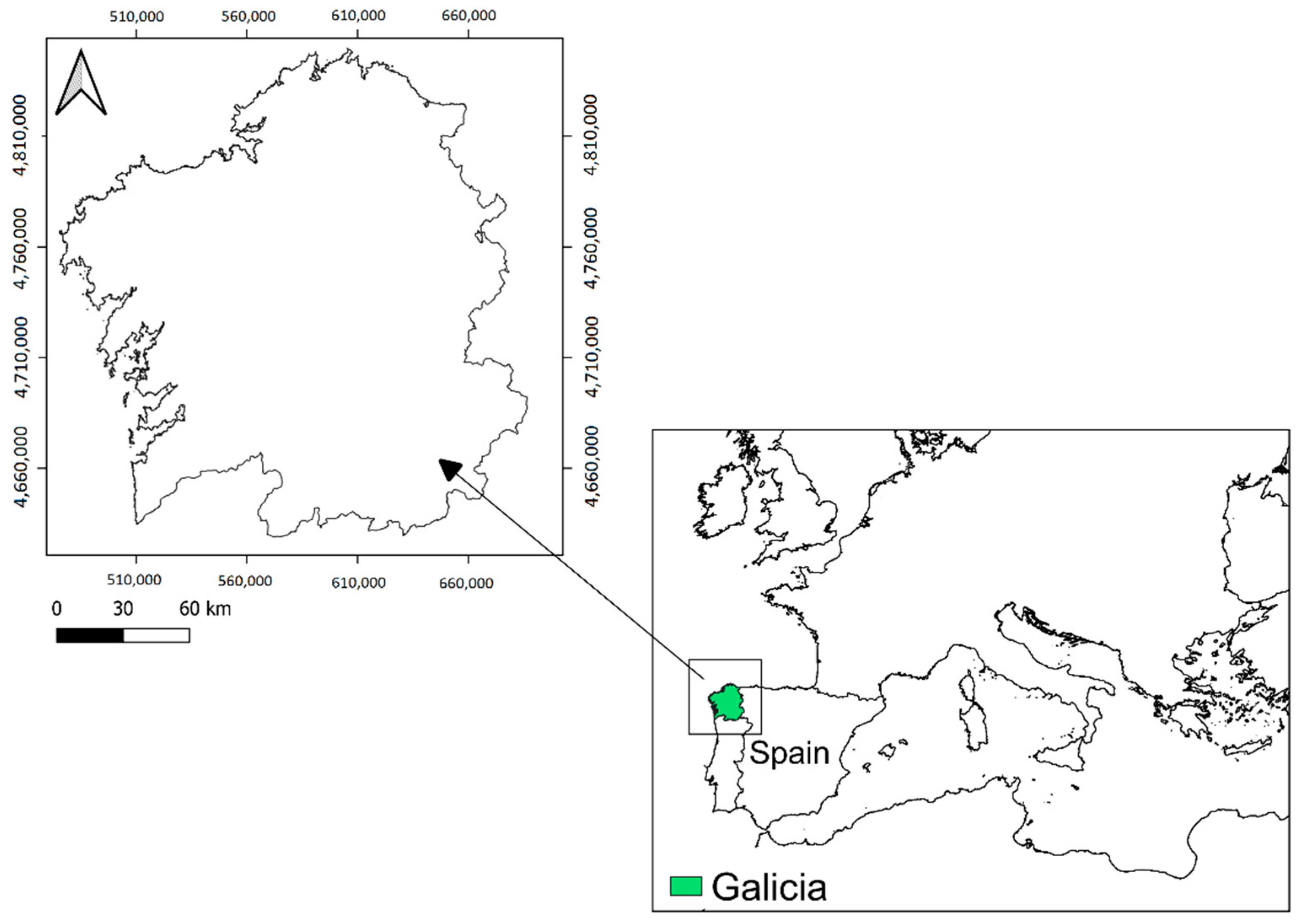
This study included the entire region of Galicia, comprising a total of 29.574 km2 (Figure 1). The altitude in Galicia ranges from sea level to nearly 2000 m and the topography includes plains as well as mountain areas with steep valleys [51]. Galicia has two types of climate according to the Köppen–Geiger classification, the Csb (Mediterranean-Oceanica climate) and the Csa (Mediterranean climate) [52].

Figure 1.
Study area: Galicia (Northwest of Spain).
According to the Spanish official cartography, 69% of Galicia is covered by forestland (the forest terrain, according to the Galician forestry sector authorities, includes woodlands and shrublands) [48]. The dominant tree species are three species of pine (Pinus pinaster, Pinus radiata, Pinus sylvestris), two Eucalyptus species (Eucalyptus globulus and Eucalyptus nitens) and broadleaves (riparian species, Quercus robur, Quercus pyrenaica and Castanea sativa, among others). The 2015 analysis of the forestry sector indicates that 30% of the forestland was shrublands and rocky areas [49]. The forestry sector represents 3.5% of the Galician GDP and 50% of the timber cuts are Eucalyptus spp. followed by conifers [53]. Galician land forest is highly fragmented. According to official cadastral information, it is estimated that 162,188 ha are in cadastral parcels that are smaller than 0.5 ha [50]; this accounts for approximately 40% of the land covered by the main productive tree species in Galicia.
3. Materials
3.1. Satellite Images
A sample of Sentinel-2 images obtained on different dates were used in this study. Sentinel-2 is a constellation of two satellites (Sentinel-2A and 2B) located in the same sun-synchronous orbit, phased 180 º from one another and launched by the ESA’s Copernicus program [54]. The two satellites allow for a revisit time of five days at the equator (two to three days at mid-latitudes). They are equipped with medium-resolution multispectral cameras capable of sampling 13 bands: three visible bands and a 10 m near infrared (NIR) band, four vegetation red edge bands, two 20 m shortwave infrared (SWIR) bands, and three 60 m bands designated for performing cloud masks and atmospheric corrections [55].
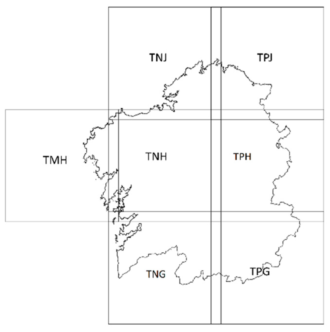
Level-2A Sentinel-2 products were used, which provide Bottom of Atmosphere (BOA) reflectance images. Each Level-2A product provides data for a 100 × 100 km2 tile in cartographic geometry (UTM/WGS84 projection). Seven tiles are needed to cover the whole region of Galicia (TMH, TNG, TNH, TNJ, TPG, TPH and TPJ). Their distribution is shown in Figure 2. It is worth noting that there are some tiles which encompass only a small portion of the surface area of Galicia; this is the case, for example, for the coastal tiles TMH and TNJ. The images used in this study date from 2019. Images were download from the Copernicus Open Access Hub [56].
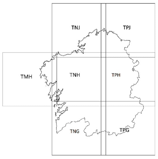
Figure 2.
Distribution of the 100 x100 km2 Sentinel-2 tiles in Galicia.
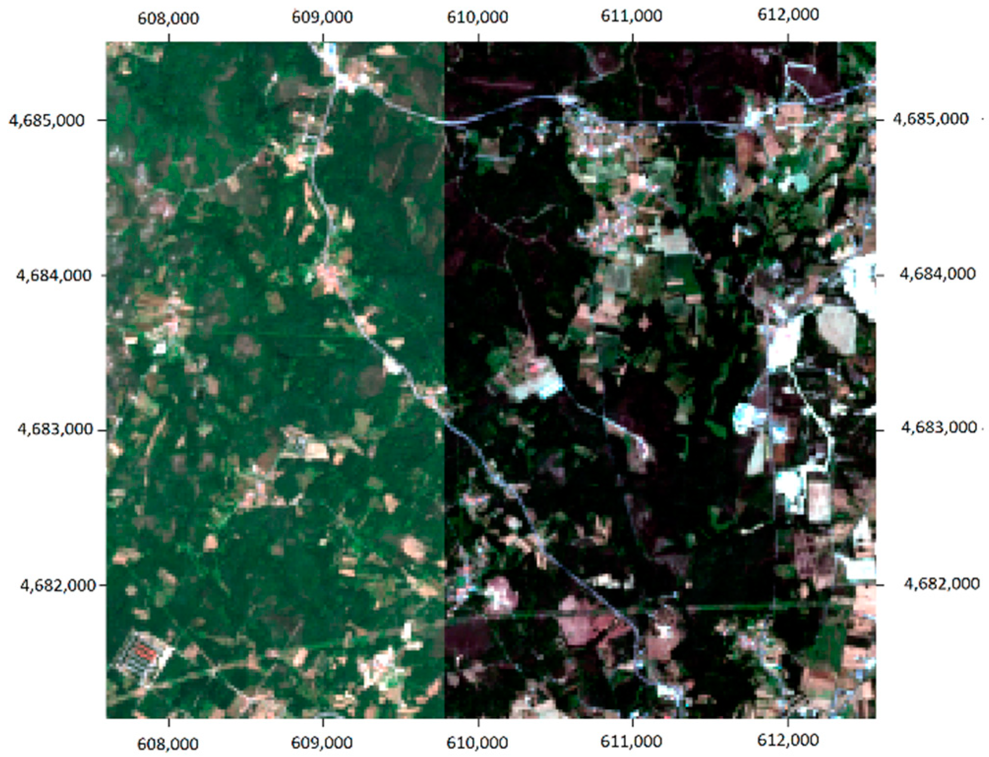
Level-2A Sentinel-2 products include geometric, radiometric and atmospheric corrections. Image pre-processing should be avoided as much as possible in order to develop the simplest methodology and make the method feasible for forest managers and decision makers. However, the downloaded images were visually analyzed, since spectral differences between contiguous tiles in Sentinel-2 products with Level-2A corrections were reported by Kukawska et al. [57], and due to the fact that this phenomenon could compromise results. Differences in radiometric values were noticeable. An example of this is shown in Figure 3. It shows the images (with RGB color compositions) from two neighboring tiles. Both images were captured on the same date (19/07/2019) and with the same satellite (Sentinel-2B).

Figure 3.
RGB color composition of TNG and TPG in the overlapping area (TPG is superimposed to TNG). Tile acquisition date: 19/07/2019. Tile acquisition hour: 11:21:19. Acquisition satellite: Sentinel-2B.
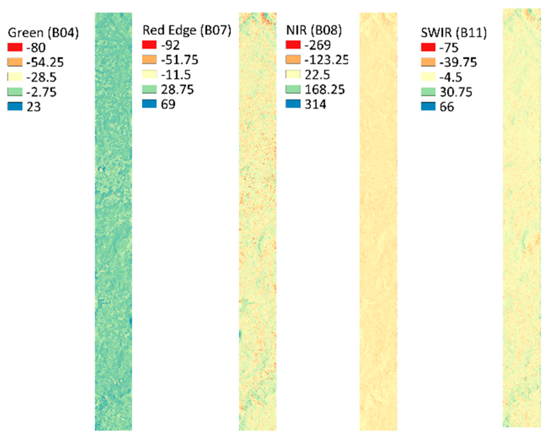
Considering that the radiometric resolution of the Sentinel-2 MSI Instrument is 12-bit [55], light intensity values can range from 0 to 4095. However, the effective range is smaller for all bands. The level of discrepancy between the tiles was quantified by subtracting the digital values between pairs of neighboring images taken on the same date (F(x) = TNG − TPG). Figure 4 shows the results for TNG and TPG images, both obtained on 19/07/2019. The difference in digital values ranges from 275 to 314, depending on the spectral band analyzed. Consequently, the radiometric discrepancies among different tiles ought to be considered relevant.
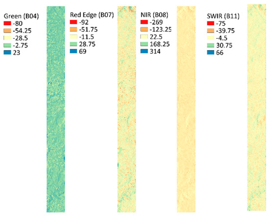
Figure 4.
Subtraction values for the overlapping area between the TNG and TPG Sentinel-2 tiles. Tile acquisition date: 19 July 2019. Acquisition satellite: Sentinel-2B. From left to right: B04, the green band of the visible spectrum; B07, Red Edge Region; B08, Near Infrared Region (NIR) band; B11, Shortwave Infrared Region (SWIR).
3.2. Reference Data
High resolution aerial orthorectified images, specifically, images from the Spanish National Program of Orthoimages (PNOA) [58], were used in the training and verification steps of the methodology. PNOA images are open-access data available on the Spanish Cartographical Institute’s (IGN) website [51]. They were obtained through a photogrammetric flight performed in 2017. The pixel size is 0.25 m and they have a georeferencing error of RMSEx,y <= 0.5 m. Google StreetView [59] was used to complement the reference data.
3.3. Hardware and Software
The computer used in this study was a Surface Pro 7. It has an Intel(R) Core (TM) i7-1065G7 CPU@ (1.30GHz 1.50 GHz) processor. It has a 16 GB RAM installed and a 64-bit operating system.
R software was utilized for the entire workflow of this study [60]. It is a free software designed to provide open-access tools to perform statistical analysis of data.
4. Methodology
This section is divided into five sub-sections. The first one describes the general methodology; the others provide a description of the methodological variables analyzed and how they were tested.
4.1. General Description
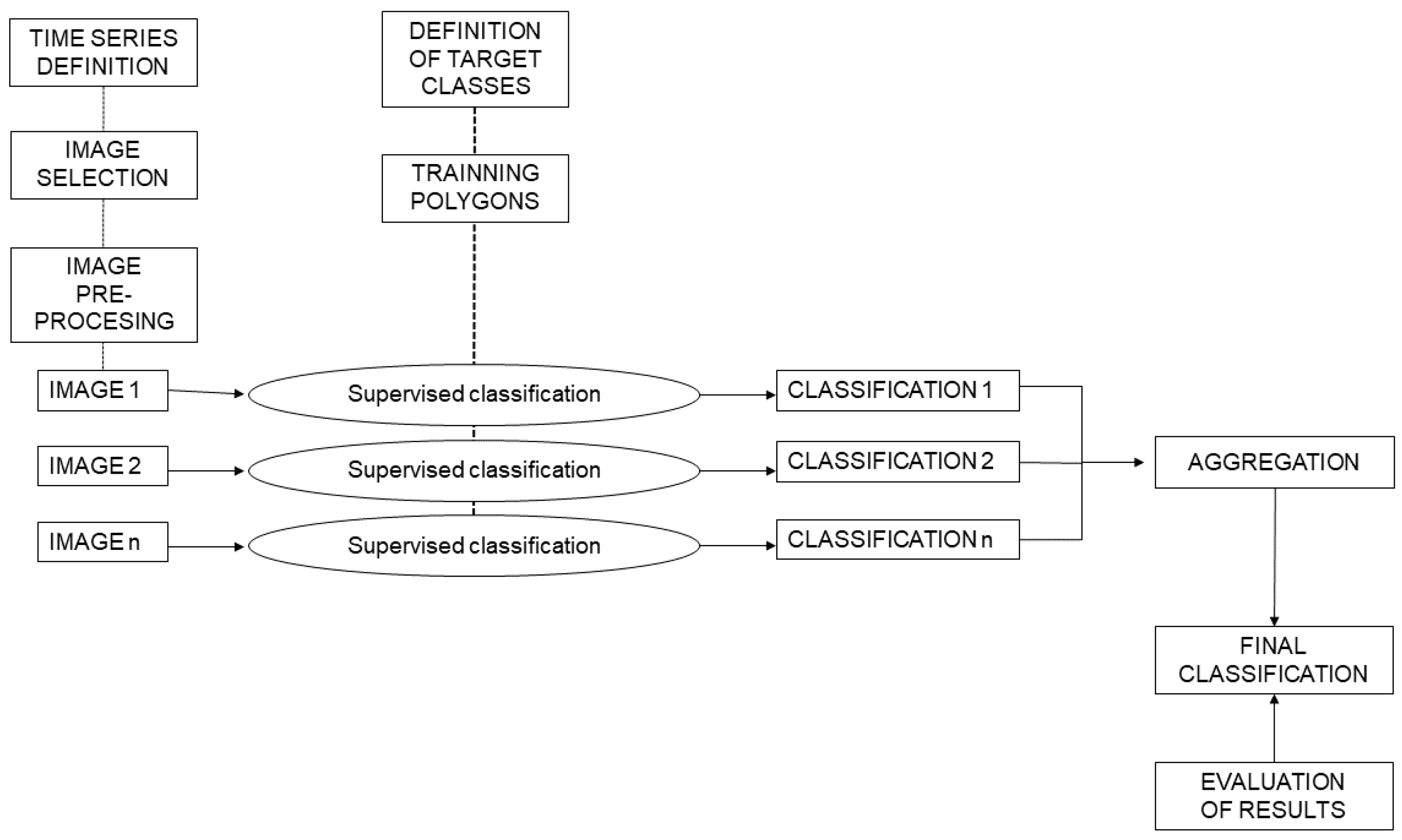
The methodology is designed to exploit the multi-temporal dimension that the Sentinel-2 satellites provide. It is based on the method developed by Lewiński et al. [22] which allows for the optimization of land-cover detection avoiding cloud-cover-related problems. It can be summarized as follows: supervised classifications are performed independently on each image from a given time series and then they are aggregated using decision criteria. The methodology can be broken down into several separate steps:
- Definition of the target classes.
- Definition of the time period for the analysis.
- Image evaluation, selection and preprocessing.
- Collection of training areas.
- Generation of single date classifications.
- Aggregation of single date classifications.
- Evaluation of results.
A diagram of the procedure followed is presented in Figure 5.

Figure 5.
Diagram of the methodological approach followed to obtain the forestry-oriented land cover map of Galicia.
The definition of the target classes is in line with the characteristics of the vegetation in the study area and is intended to meet the needs of the forestry sector. In this case, eight land cover classes were defined. See Table 1.

Table 1.
Description of target land cover classes.
The second step is the definition of the time period. In order to optimize the multi-temporal approach, the entire phenological period for the vegetation in the region under study must be considered. In this case, the time series contemplated is represented by 12 images that cover the whole year of 2019. One image from each month was selected. One of the important objectives of this methodology is to obtain a cloud-free classification. For each image to be processed, a maximum threshold value of 50% for Cloud Cover Percentage (CCP) was established. In cases where a given month had multiple images that met this criterion, the image with the lowest CCP was selected. On the other hand, if a certain month had no images to satisfy the cloud-cover criterion, an image at the end of the previous month or at the beginning of the following month was selected. For each Sentinel-2 tile, Table 2 shows the date of the selected images, their CCP, their Cloud Shadow Percentage (CSP) and their Dark Features Percentages (DFP).

Table 2.
Sentinel-2 images downloaded and used for land cover map creation. Images are grouped according to their tiles and their acquisition dates. The cloud cover percentage (CCP), cloud shadow percentage (CSP) and dark features percentage (DFP) are listed for each image.
The image preprocessing step involves masking out the pixels covered by clouds and clouds shadows. This step was done by applying the 20 m cloud mask provided by the Level-2A of Sentinel-2. As a result, all of the pixels identified as clouds or cloud shadows were reassigned NoData values for all of the bands of all of the Sentinel-2 images.
The delineation of training area polygons for the target classes was achieved through photointerpretation. For this purpose, a combination of high resolution orthorectified images (from PNOA) [58] and Sentinel-2 images with different color compositions was used. Whenever it was possible, Google StreetView images were used to aid in the photointerpretation process. Polygons were distributed across each individual tile. The distribution within each tile was stratified, aiming to select approximately the same number of pixels of each class and to avoid a biasing of the selected areas in a certain location. The training polygons for the different forestry classes (Eucalyptus spp., Conifers, Broadleaves and Shrubs) in any given tile included a minimum of at least 2000 20 × 20 m2 pixels. The defined training polygons encompass a total of 243,469 pixels, GSD 20 m, corresponding to 0.27% of the entire Galician surface area. They were distributed among the seven tiles that cover the study area, comprising at least 0.15% of the analyzed surface area of each tile. In tiles with smaller surface areas, this percentage is higher; for instance, it is 0.58% in TNJ. Table 3 contains the number of training pixels for each individual tile. Table 4 presents the number of training pixels per class and per tile. The sample size was over 2000 pixels per tile for all forest classes, except for the broadleaf class in TMH. In the case of the TPG tile, Eucalyptus spp. cover is scarce, so no training pixels were considered. In relation to the non-forest classes, it is worth noting that the Bare soil class was the most problematic in terms of acquiring a sufficient amount of training data.

Table 3.
For each Sentinel-2 tile: Number of 20 × 20 m2 pixels within Galician territory, number of 20 × 20 m2 pixels used as training pixels, and percentage of the total Galician surface area covered by training data.

Table 4.
Number of 20 × 20 m2 training pixels by tile and class used to perform all of the supervised classifications presented in the study.
The fifth step is the generation of one supervised classification for each image that comprises the multi-temporal series. The algorithm used was RF [61], a machine learning algorithm that bases its classification on the creation of multiple decision trees. These trees are combined such that each tree depends on the values of a random vector sampled independently and with the same distribution for all trees in the forest. The outputting class is the mode of the classes of the individual trees. The supervised classification starts with the creation of these trees based on the information from the training data. As a result, the algorithm creates a model that is applied to each individual pixel in the image to predict its corresponding class. Additionally, RF allows for the estimation of the probability that each pixel belongs to each class. RF was implemented using the randomForest R package [62]. The default configuration parameters were used (number of trees: 500, and number of features used in each split: 3), as it has been shown in several studies that changing RF parameters has little influence on classification accuracy [37,38].
The bands that were used in the supervised classification were those with 10 m and 20 m pixel sizes (B02, B03, B04, B05, B06, B07, B08, B8A, B11 and B12). To perform the classification, bands must have the same resolution. The bands with 10 m resolution were aggregated using nearest neighborhood interpolation.
The sixth step consists of designing an aggregation criterion to obtain one single classification image that contains all of the vegetation covers in the study area in 2019. Lewinski et al. [22] present several aggregation criterions. Two of them will be applied. Once the criterion is selected, the multiple classifications are combined to obtain the final single one. The resulting map is highly dependent on the aggregation criterion used.
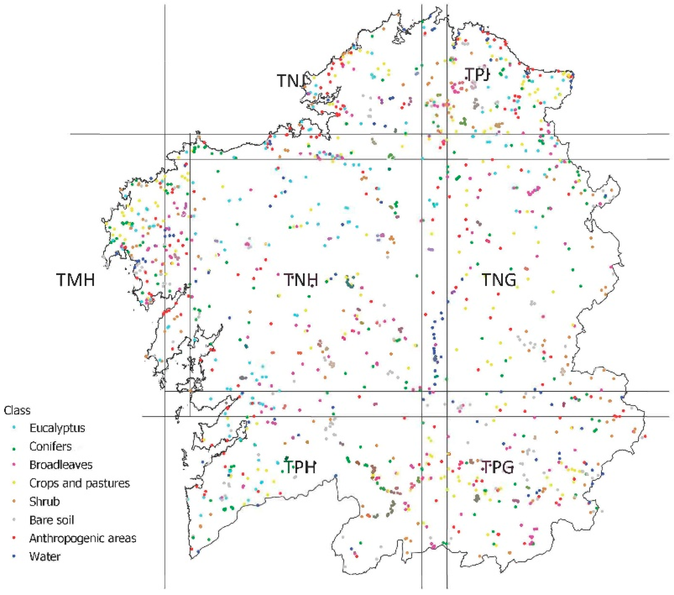
Finally, the result of the classification is evaluated. For this purpose, a set of 1628 points were selected within the study area, intending to spread the sample evenly among the study area. Their corresponding vegetation covers were identified through photointerpretation of PNOA images [59]. The photointerpretation was supported whenever possible by Google StreetView images. A set of 30 points (minimum) per tile for each forestry class was created to obtain a stratified verification sample. In non-forestry, classes this number was also sought but it was not restrictive. In terms of points per class, a total of 190 for Eucalyptus spp., 280 for Conifers, 281 for Broadleaves, 207 for Shrubs, 211 for Crops and Pastures, 189 for Bare soil, 153 for Anthropogenic areas and 117 for Water were obtained. The Eucalyptus spp. class had few verification points in comparison to other tree classes, but it should be noted that this species is not present in the Southeastern region of Galicia. Distribution of verification points is presented in Figure 6.
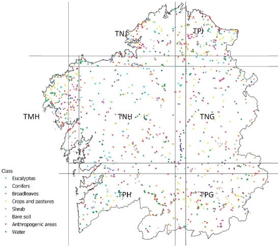
Figure 6.
Distribution of verifications points.
Using these reference points, a cross-verification was performed of the individual pixels where each point lies; the photo-interpreted class was compared with the classification result. Afterwards a confusion matrix was built which was subsequently used to calculate the following metrics:
- Overall Accuracy (OA): calculated by summing the number of correctly classified sites (the diagonal of the matrix) and dividing by the number of reference sites. This value indicates the proportion of the reference sites that was correctly classified.
- Producer’s Accuracy (PA): the result of dividing the number of correctly classified reference points in each category by the total number of reference points for that category. It corresponds to the map accuracy from the point of view of the map maker. It represents how often real features on the ground are correctly shown on the classified map or the probability that a certain land cover of an area on the ground is properly classified.
- User’s Accuracy (UA): computed by dividing the number of correctly classified pixels in each category by the total number of pixels that were classified for that category. This value represents the reliability of the map or the probability that a pixel classified into a given category actually represents that category on the ground.
- F-1 Score: a weighted average of the producer’s and user’s accuracy.
- Kappa Index: compares the accuracy obtained in the classification to the accuracy that would be obtained randomly. It is calculated as the difference between the total accuracy (OA) and the accuracy that would be obtained by a random classification, divided by one minus the accuracy that would be obtained by a random classification.
- p-value associated to Kappa Index: probability that the Kappa Index measures the evidence against the null hypothesis (H0: agreement is due to chance).
The next four sections present and evaluate four parameters that can potentially affect the accuracy and efficiency of this methodology.
4.2. Aggregation Method
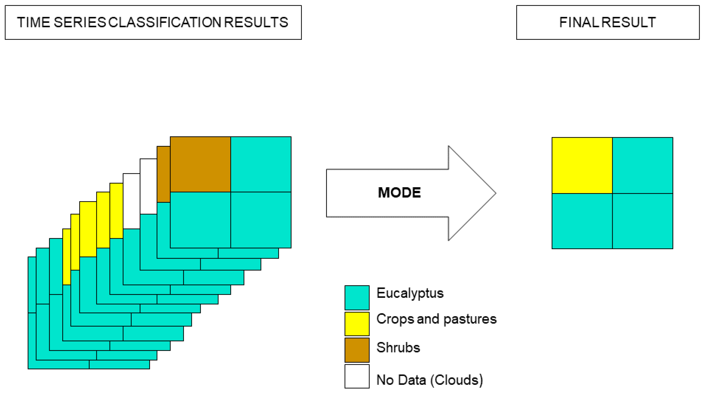
Two different aggregation methods were tested in this study in order to select the most suitable one in terms of accuracy and efficiency. They were described by Lewiński et al. [22] (2017): Plurality voting and DivByAll. In their work, Lewiński et al. [22] showed that using these different criteria for aggregation could generate different results. The first method, Plurality voting, consists of assigning as the final class the most commonly occurring class among all of the classes identified throughout the time series. In this study, the Plurality voting method was implemented using an R software function that selects the mode value. A diagram of the method is shown in Figure 7.

Figure 7.
Diagram of the Plurality voting aggregation method used to aggregate the classification results of the different individual classifications throughout a time series to obtain one final classification. Method developed by Lewiński et al. [22] (2017).
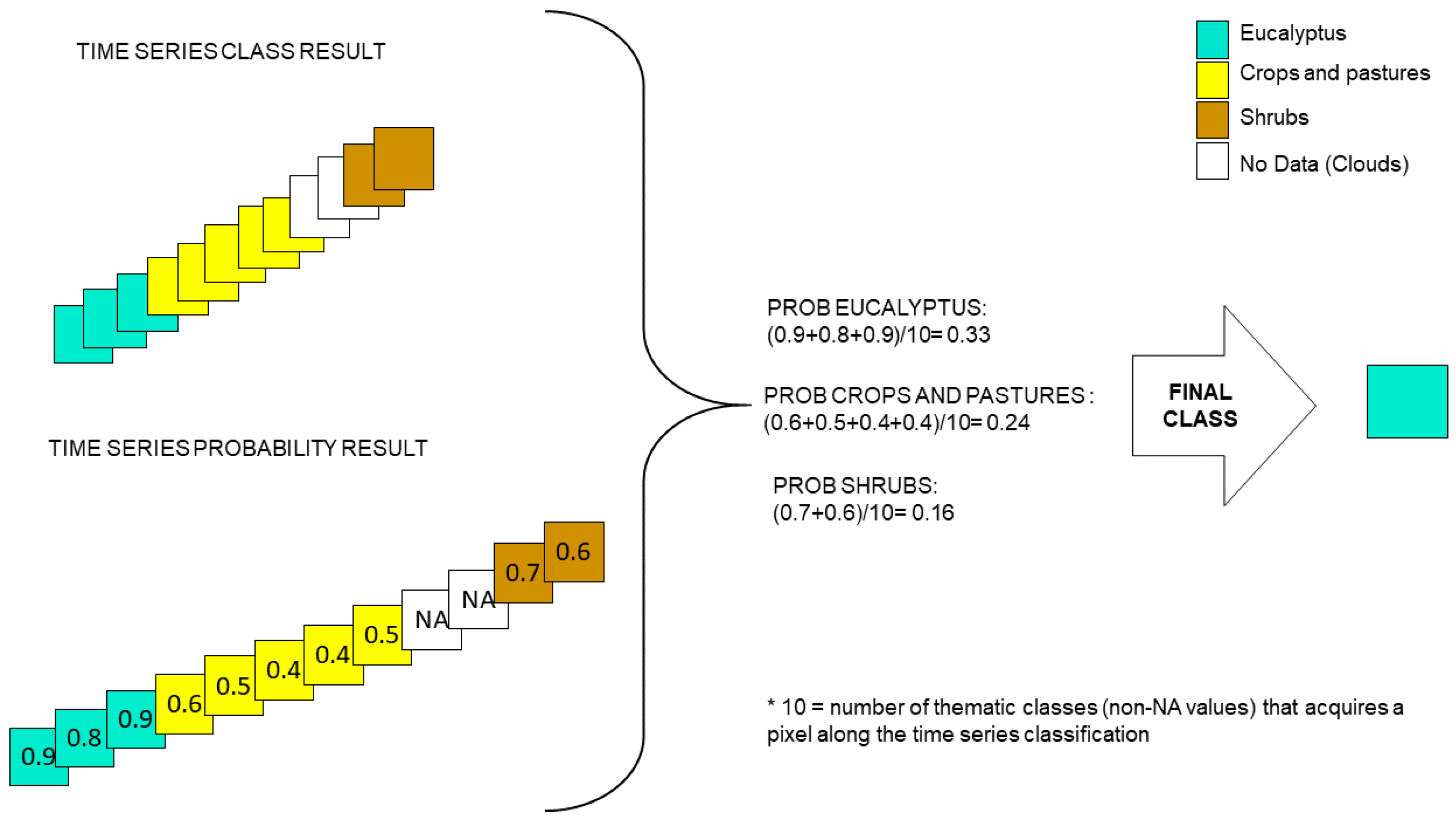
The second aggregation method, DivByAll, bases the aggregation on the values that RF gives for the probability that a pixel belongs to a given class. These probability values correspond to the fraction of the total number of trees which vote for a specific class. Then, the values for the probability that a pixel belongs to a given class in each of the different images throughout the time series are summed and divided by the total number times that classes were detected within that time series (this is to account for NA values, which come from clouds, so that they do not skew the probability that a pixel belongs to a certain class). The class yielding the highest probability is the class that is ultimately assigned. A diagram of the method is presented in Figure 8.

Figure 8.
Diagram of the DivByAll aggregation criteria used to aggregate the classification results of each individual image in the time series to obtain a final classification. Adaptation from Lewiński et al. [22] (2017).
4.3. Random Forests Training and Model Creation
Two different approaches were tested for creating the RF model considering the radiometric divergence among the Sentinel-2 tiles in the study area. It is well known that the radiometric coherence of images in a mosaic is a requisite for performing a supervised classification. It is also understood that accuracy results are dependent on the amount of training data used [38]. Larger training datasets can potentially correlate to higher accuracy levels. In this study, two different approaches were considered, each one compromising one of these two conditions.
The first RF modeling approach consisted of creating an independent model for each tile using only the training areas that belonged to that tile. This approach is a way to minimize the impact of the radiometric divergences explained in Section 3.1. [63]. The second RF modeling approach combined the training areas of all the tiles to create one single common model. The advantage of this method is that it allows for an increase in the amount of input training data.
Both approaches were applied for the entire surface area of Galicia with a 20x20 m2 spatial resolution. The classifications of all of the months were aggregated using Plurality voting criteria. A cross verification was performed on both classifications using the verification points. In both classifications, a confusion matrix was produced for each tile. The results were analyzed in order to determine which method conferred greater accuracy.
4.4. Spatial Resolution
Two classifications were performed for the entire surface area of Galicia with two different spatial resolutions: 20 m and 10 m. As mentioned before, one of the main strengths of Sentinel-2 compared to other open-access satellites (ex. Landsat) for land cover map production is its spatial resolution [5]. Most Sentinel-2 channels are available at a resolution of 10 or 20 m. A preliminary step in any classification process is the standardization of the units of resolution used by the different bands. Map production at a 10 m spatial resolution is optimal when dealing with spatial information contained in 10 m channels [20,35]. However, using this pixel size requires increased processing time since 20 m bands have to be resampled at 10 m. Computing time increases as well as the number of pixels in each scene is quadrupled. Additionally, 10 m resolution products entail larger storage demands which could be a problem when managing data for large areas.
According to different studies, the reflectance that allows for the optimum differentiation between vegetation classes is that of the 20 m bands (the three red edge bands, the narrow NIR band and the two SWIR bands) [5,14,20], which implies that the 10 m bands have the reflectance that contributes the least to the classification. This leads to the hypothesis that a 10 m classification may be only slightly more accurate than a 20 m classification, meaning that the processing time and increased storage demands may not be worth the trouble.
Two classifications were performed, one using the bands at 10 m resolution and another one at 20 m resolution. In the 10 m resolution classification, 20 m band cells were divided into two cells to convert them into 10 m bands. In both cases, the modeling approach used was the single RF modeling and the aggregation criterion was Plurality voting. The results were compared in terms of accuracy, processing time and storage requirements. A cross verification was performed in each case using the verification points. Confusion matrices with UA, PA and OA were also created.
5. Results
5.1. Aggregation Method
The results for the classifications of the TNH tile using the two proposed aggregation approaches are shown in Table 5 and Table 6. Table 5 presents the confusion matrix for the classification using the Plurality voting aggregation method. Table 6 shows the results for the classification using the DivByAll aggregation method. The accuracy metrics are similar for both methods: the OAs are 91.8 and 92.1, respectively. The Producer’s and User’s accuracies differ by less than 3 percentage points in all cases, and in the majority of cases by less than 1 percentage point. The F-1 score is not lower than 0.8 for any of the classes in either method. The Kappa index is around 0.9 in both cases.

Table 5.
The Confusion matrix obtained for the final classification of the TNH tile produced using the Plurality voting aggregation method. Producer’s Accuracy (PA), User’s Accuracy (UA), Overall Accuracy (OA), F-1 score (F-1), Kappa Index (KI) and its derived p-value (p-value). Classes: Eucalyptus spp. (1), Conifers (2), Broadleaves (3), Crops and pastures (6), Shrubs (7), Bare soil (8), Anthropogenic areas (9) and Water (10).

Table 6.
The Confusion matrix obtained for the final classification of the TNH tile produced using the DivByAll aggregation method. Obtained metrics: Producer’s Accuracy (PA), User’s Accuracy (UA), Overall Accuracy (OA), F-1 score (F-1), Kappa Index (KI) and its derived p-value (p-value). Classes: Eucalyptus spp. (1), Conifers (2), Broadleaves (3), Crops and pastures (6), Shrubs (7), Bare soil (8), Anthropogenic areas (9) and Water (10).
Producing the TNH classification aggregating by Plurality voting took a total of 5 h 40 min 35 s, while producing the TNH classification aggregating by DivByAll took a total of 16 h 17 min 2 s. The additional step needed (creating the probability rasters) is what most increased the production time (an increase of 5 h) (see Table 7).

Table 7.
The processing time to obtain the TNH land cover classification using the two different aggregation methods (Plurality voting and DivByAll).
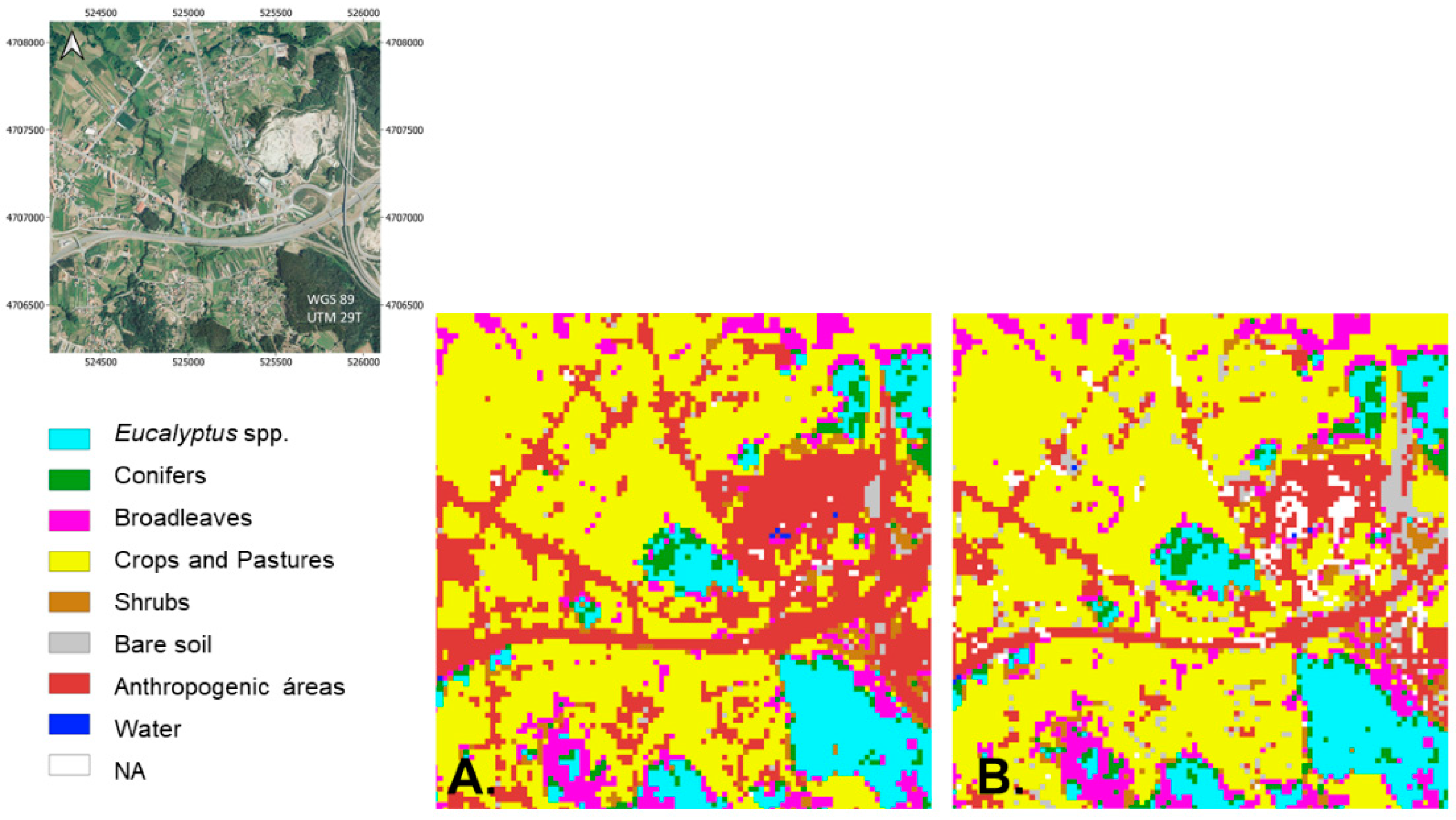
Upon visual inspection, mapping differences were observed between the two classifications in the Anthropogenic areas. In the classification obtained using the DivByAll aggregation criteria. No Data values derived from the cloud mask appear while these are more commonly avoided using the Plurality voting criteria. An example is shown in Figure 9.

Figure 9.
Two land cover classification results of an Anthropogenic area using different aggregation criteria. (A) Classification obtained using the Plurality voting aggregation criteria. (B) Classification obtained using the DivByAll aggregation criteria. Reference true color image: orthorectified aerial image (PNOA) [49].
5.2. Random Forests Training and Model Creation
The results for the accuracy metrics derived from the two RF modeling approaches are shown in Table 8. Specifically, the OA, PA, UA and Kappa Index obtained in each of the confusion matrices are included. The average overall accuracy in the case of the single model was 91.55%, while it was 89.73% when using the independent model method. Comparing the accuracy for each tile, the single model method yielded accuracy scores 8 percentage points higher than the independent model method in the case of the TMH tile. Only in one tile (TNG) was the OA for the single model method lower (2% lower) than the OA for the independent model method. The Kappa Index is high in all scenarios (between 0.78 and 0.94). It is either higher or does not vary when using the single model method, except for in the case of the TNG tile, where it is 0.02 points lower.

Table 8.
Comparison of the accuracy metrics obtained from the cross verification of the two different classifications created following the different model creation strategies for the entire surface area of Galicia. M_TILE: An independent model for each tile. M_ALL: A single model for the entire surface area of Galicia. Metrics presented: Users Accuracy (UA), Producer’s Accuracy (PA) and Overall Accuracy (OA), F-1 score, Kappa Index (KI) and its derived p-value (p-value). Classes: Eucalyptus spp. (1), Conifers (2), Broadleaves (3), Crops and pastures (6), Shrubs (7), Bare soil (8), Anthropogenic areas (9) and Water (10).
Considering the forestry-related classes (Eucalyptus spp., Conifers, Broadleaves and Shrubs), differences are minimal in most cases (less than 0.1%); where they are not, the single model also results in better metrics. The most noteworthy improvement is the increase in the PA by 36.3 percentage points for the Eucalyptus spp. class in the TNH tile.
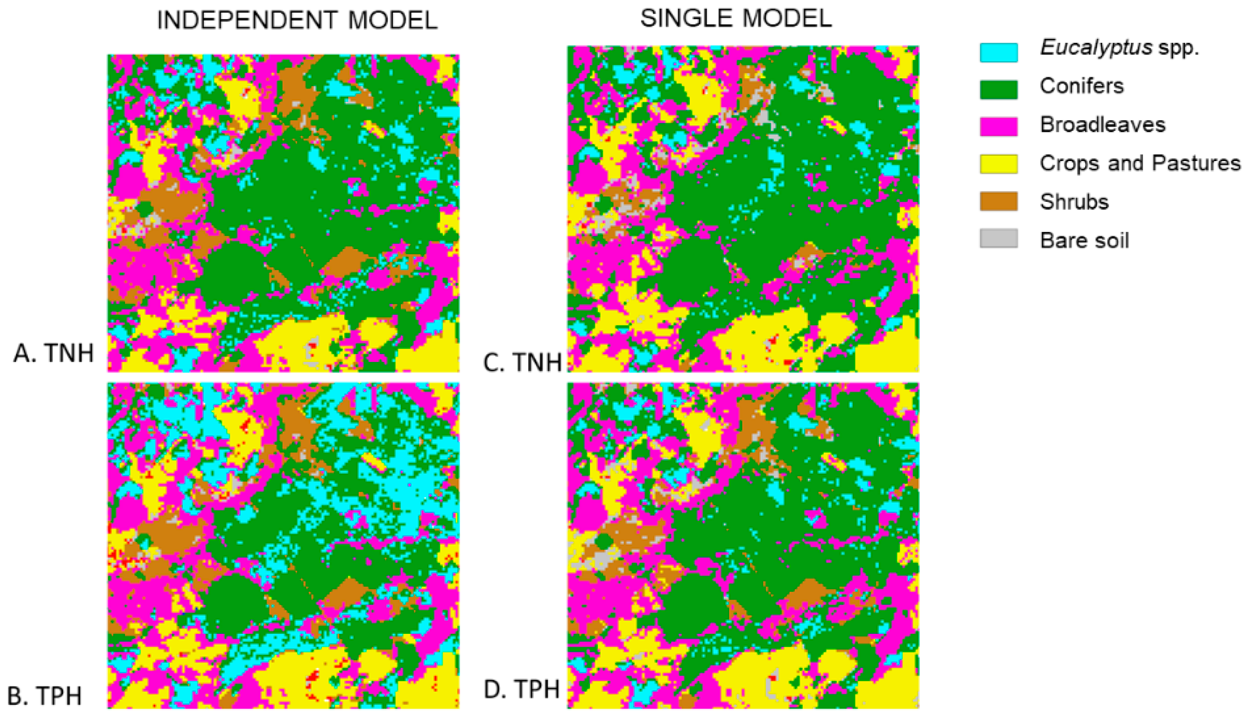
Upon visual inspection, it was observed that when independent models were created, classification results in overlapping areas differed between tiles. However, when a single model was used for all of the tiles, the classifications in overlapping areas closely matched. An example is shown in Figure 10.

Figure 10.
Land cover classification results of contiguous tiles for an overlapping area. (A–D) represent the same area. (A,B) were obtained using an independent model for each tile. (A) represents the results obtained for the TNH tile. (B) represents the results obtained for the TPH tile. (A,B) are different. (C,D) were obtained using one single common model for all of the tiles. (C) represents the results obtained for the TNH tile. (D) represents the results obtained for the TPH tile. (C,D) are quite similar.
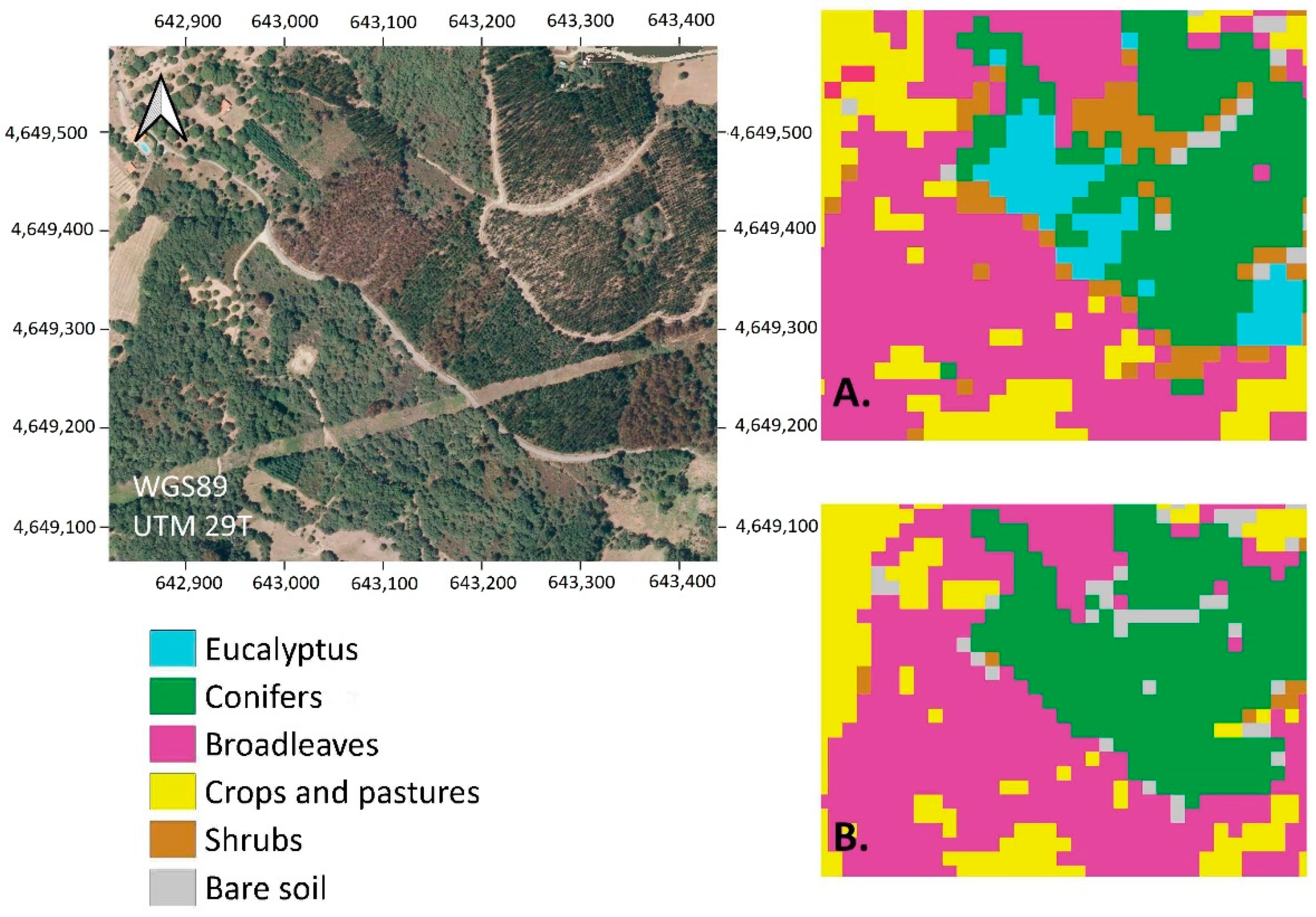
Visual inspection also revealed that, in using the single model approach, it was possible to map small areas belonging to the Eucalyptus spp. class on the TPG tile. However, when the independent modeling approach was used, Eucalyptus spp. could not be mapped on this tile and were assigned instead to the Conifer class. An example can be seen in Figure 11.

Figure 11.
Land cover classification results for the TPG tile using different approaches in the modeling step of the supervised classification. (A) Results from the single model approach to predict the final class on all tiles. (B) Results obtained using an independent model for each tile using only the training areas defined within that tile. The presence of Eucalyptus spp. on the TPG tile were not mapped in the second case. Reference true color image: orthorectified aerial image (PNOA) [49] (MTMAU 2021).
5.3. Spatial Resolution
Table 9 shows the confusion matrix for the classification at 20 m and Table 10 for the classification at 10 m. The OAs for both classifications are identical. The F-1 score values for the forestry classes are 1 percentage point higher in the 20 m classification. The differences in PAs between the two classifications are less than 2% for the forestry-related classes (Eucalyptus spp., Conifers, Broadleaves and Shrubs). The greatest difference was in the Eucalyptus spp. Class, where the PA was 1.6 points higher for the classification at 20 m. The greatest differences in PA values were in the Bare soil class and the Anthropogenic area class. For these two classes, higher accuracy results were obtained using a10 m resolution. The UA for the forestry-related classes is always greater in the classification produced at 20 m. In these classes, it differs by a maximum of 2.7 percentage points in the case of the broadleaf class. Greater differences can be seen in the Anthropogenic area class where the OA is 4% higher in the classification obtained at 10 m.

Table 9.
Confusion matrix of the cross verification performed for the classification produced at 20 m to decide the optimal resolution for producing regional land cover maps. Obtained metrics: Users Accuracy (UA), Producer’s Accuracy (PA) and the Kappa Index (KI). Eucalyptus spp. (1), Conifers (2), Broadleaves (3), Crops and pastures (6), Shrubs (7), Bare soil (8), Anthropogenic areas (9) and Water (10).

Table 10.
Confusion matrix of the cross verification performed for the classification produced at 10 m to decide the optimal resolution for producing regional land cover maps. Obtained metrics: Users Accuracy (UA), Producer’s Accuracy (PA) and the Kappa Index (KI). Eucalyptus spp. (1), Conifers (2), Broadleaves (3), Crops and pastures (6), Shrubs (7), Bare soil (8), Anthropogenic areas (9) and Water (10).
The time required to process the data in order to obtain the Galician land cover map at each resolution was calculated. Processing at 10 m took approximately three times longer (approximately 92 h were needed to obtain the whole classification at 20 m and 238 h at 10 m).
Regarding storage demands, the Galician rasters, which contain the land cover maps at 20 m and 10 m resolution, occupied 915 MB and 3.57 GB, respectively.
6. Discussion
6.1. Time Series Selection
Varying criteria were found in the specialized literature for the definition of the time series and image selection strategy. Previous studies took the orography of the study area, the vegetation phenology and the frequency of land cover changes into account when selecting the time period of the multi-temporal image series [64]. For example, short time series have been used in studies of mountainous areas where mountain shadows, permanent snow and cloud cover hide the vegetation, making it impossible to be mapped [65]. Given the vegetation and topography of Galicia, it was feasible and preferable to use one image per month.
In relation to the image selection strategy, Malinowski et al. [63] selected two images per month during the growing season and one image per month for the remaining months. The least cloudy image was frequently selected from all of the available images for a month [22,63,66]. Some studies heed only the criterion of selecting the least cloudy image, admitting images with a CCP anywhere between 0% and 100% [22]. Others establish an additional criterion, such as cloud cover threshold, in order to ensure the accuracy of the method. The CCP threshold value depends on the nature of the climate in the study area as well as on the size of the study area. For example, Malinowski et al. [63] map a large area with climates that frequently have cloudy weather (Europe); for this context, they select a 50% threshold. The present study also covers a relatively large area which includes regions with an Atlantic climate, meaning that Autumn and Winter are characterized by significant cloud cover. Therefore, a relatively high CCP threshold is also necessary (50%). A more conservative value is used in Belcore et al. [66] (10%) since they aimed to map a smaller region and included only summer images in their time series.
6.2. Reference Dataset
The creation of training areas was the most time-consuming step in the described methodology, since all training areas had to be manually delineated through photointerpretation. The training dataset size is considerably large in order to ensure the minimum percentage (0.25% of the total study area) stipulated by reference studies, which indicate the training needs of the RF classifier in order to achieve high levels of accuracy in its classification [67]. However, this is a step that has room for improvement. Some other previous studies suggest the use of pre-existing land cover databases, for example Corine Land Cover or National databases [21,63,68]. However, the available datasets in Spain do not have enough detail for all regions. This is the reason why in this study the manual approach was followed. In future research, the implementation of a semi-automatic approach will be studied. An example is the methodology described by Gromny et al. [69] where the training process is initiated by an operator, who defines the initial spectral characteristics, and then continued via an automatic process where areas with similar spectral characteristics are identified.
It should be mentioned that the use of photointerpretation to define the training polygons may involve some class mislabeling due to potential operator errors. Operators ought to be well trained in photointerpretation in order to minimize this kind of error. Alternatively, obtaining training data through field work could solve this problem. However, it would be quite time-consuming and expensive for large study areas. Furthermore, according to Mellor et al. [70] studies, some mislabeling in training data might not affect the RF classification accuracy as they have shown that the RF classifier is relatively insensitive to this phenomenon.
Photointerpretation was used as well to obtain verification points, the significant strengths of this method being its low cost, its applicability to differing terrain conditions (it can be used for any terrain slope and in cases of shrub closure), and the minimum amount of time elapsed between reference and classified images. However, photointerpretation complicates the design of the sampling procedure as there are portions of the population of pixels which are difficult to label and, as such, were not included in the training dataset nor in the evaluation dataset. This hinders planning a sample design which takes the inclusion probabilities of the verification points into consideration (i.e., it hinders performing a random sampling). According to Stehman, knowledge of the verification points’ inclusion probabilities would be ideal in order to perform a design-based inference [64,65,71]. Comparisons between different classification techniques using the presented dataset are valid within the scope of the data collected. Although it would be ideal to apply any of the above-mentioned strategies to obtain the verification points, it would mean overlooking the principle of cost-effectiveness [70]. In fact, multiple other land cover studies performed over large areas have faced this same problem, and in these cases accuracy metrics were calculated based on verification samples for which inclusion probabilities were unavailable. They were calculated by relying on field inspection campaigns [11,15,16,17,43,44,45], or on fieldwork only in accessible areas [40] or through photointerpretation of feasible areas [19]. Future studies could be done to explore the accuracy of the map outside photo-interpretable areas. Additionally, the reliability of the map could be explored by studying random-forest-derived probabilities [65].
6.3. Aggregation Criteria
The results of this study regarding the accuracy of aggregation methods confirm the findings of Lewiński et al. [22]: Plurality voting and DivByAll provide similar accuracy metrics. The difference between the two lies in the incidence of cloud masking and efficiency. In the Plurality voting aggregation method, NA values are frequently assigned to Anthropogenic areas. These NA values are pixels classified as clouds by the Sentinel-2 Level-2A product cloud mask. Previous studies have already reported this problem [57]. However, Plurality Voting seems to be the most efficient aggregation method for mapping large areas, since processing time greatly increases when using the DivdByAll method (which takes 5 h per tile). This is especially true when the main focus is vegetation cover and not Anthropogenic surfaces. In fact, another study which follows the Lewiński et al. [22] document, performed by Belcore et al. [66], also uses individual classifications to aggregate data according to the most frequent pixel values. Malinowski et al. [63], on the other hand, use the DivByAll method. One reason that could have led them to choose this approach was to avoid the large number of NA pixels.
6.4. Model Creation
The results reveal that the radiometric divergences among Sentinel-2 tiles are not large enough to compromise the results of the final classification. It should be mentioned that even though radiometric discrepancies could compromise the results, this could be corrected through radiometric normalization procedures [72,73]. However, it would complicate the methodology. The creation of one single model leads to highly accurate results. Furthermore, creating a single model increased the accuracy metrics for tiles which represent only a small proportion of the study area, thus illustrating the importance of the size of the training data for the RF classification [67].
Another important advantage of using this approach is that when a single model is used, the resulting classifications match in areas which overlap between different Sentinel-2 tiles. This is key when large areas are mapped, and a single coherent map needs to be obtained. Furthermore, the creation of one single model allows for the mapping of classes that are not frequent enough to define a training set in a particular tile, for example in the case of the Eucalyptus spp. class in the TPG tile. However, considering the results obtained by Malinowski et al. [63], it is possible that the single model creation approach may not be feasible for very large study areas. In such cases, independent tile modeling should be applied [63].
6.5. Spatial Resolution
The resulting classifications for the two different spatial resolutions indicate that smaller pixel size does not equate to higher accuracy. Similar accuracy metrics are obtained for the two different resolutions. In fact, for the vegetation classes, there is even a general trend towards obtaining higher accuracy metrics when using a 20 m resolution. This suggests that, as expected, the bands that bear the most weight in discriminating between vegetation classes are the 20 m bands [14], and that the resampling process changes the radiometry of these bands in such a way that it can lead to class mislabeling. Using a 10 m resolution, higher accuracy metrics are only obtained in the case of the Anthropogenic area class. This is the class that contains the most small-scale features, such as roads, that may benefit from the 10 m resolution. As this study is designed to meet the needs of the forestry sector, 20 m resolution mapping can be deemed the most appropriate. Compounded upon this is the fact that computing time and storage needs are reduced when mapping at a 20 m resolution. Nevertheless, this may only be assumed in cases where forest cover is the principal aim of classification.
6.6. Comparison with Other Large-Scale Land Cover Classifications Performed with Sentinel-2
Taking into account the previously discussed explorations of different parameters, the final classification was performed with the following characteristics: 20 m resolution bands, creating one single RF model for the classification of all of the tiles, and Plurality voting criteria to aggregate the individual classifications from the time series. High accuracy results (91.6% OA) were obtained for this classification with a high Kappa Index (0.9) with a p-value above 2.2 × 10⁻¹⁶. These are comparable with the accuracy results of other Sentinel-2-based land cover classifications for large areas. For example, the land cover map for all of Europe developed by Malinowski et al. [63] also reports high accuracy metrics, with an OA of 86.1%. It uses a methodology based on aggregating time-series classifications, similar to the methodology followed in this study.
Obtained individual metrics of target classes are also high. For example, the F-Score is never below 0.84. Vegetation classes are the ones with the highest accuracy metrics while bare soil and anthropic areas are the least accurate. This may be because they are the least abundant areas. However, increased accuracy can be seen for the individual metrics of vegetated areas. It is noticeable that crops’ UA accuracy is high (99.1). This difference could be due to some class imbalance in training data and how the RF algorithm performs in these cases, especially for the bare soil class. This problem could be solved by balancing the classes using some of the methods mentioned by Maxwell et al. [38] or by deliberately imbalancing the more challenging classes as Mellor et al. [70] suggest. In terms of forestry-related classes, all of them have high F-score values, with the shrubs class having a slightly lower value. Comparing these individual metrics with the ones obtained in other studies is difficult as target classes differ. For example, Malinowski et al. [63] discriminate between 13 different land cover classes, but they do not differentiate between the Eucalyptus spp. class and other broadleaves. This class, in particular, is essential for the Galician forestry sector, and this study serves to show that it can be successfully discriminated from other Galician broadleaves using Sentinel-2 data. Some other recent studies have analyzed the separability of the Eucalyptus spp. class using Sentinel-2 data with varying results [46,74]. The average F-1 score value obtained in this classification is higher (0.91) than the one obtained by Malinowski et al. (0.86) [63]. This difference might be mainly, because they have created different classes for crops, pastures and vineyards. These classes are combined into a single one, Crops and pastures, in this study. This grouping avoids errors distinguishing between these three radiometrically similar classes, allowing for an increase in the overall accuracy while at the same time not compromising the target information of the study, the forestry-related information.
Accurate large-scale land cover maps have been developed using different methodologies as well. For example, Griffiths et al. [41] developed a different approach to fulfilling the agricultural mapping needs in Germany. They were able to distinguish between a total of 21 different land cover classes, including 15 specific crop types, using Sentinel-2 and Landsat-8 data, but they obtained a lower OA value (76%). Another different methodology was developed by Inglada et al. [21] to create a land cover map of France. In this case, high accuracy values were obtained (k coefficients and PA above 0.8); however, they point out that their classification is highly dependent on the large amount of cloud-free imagery which they were able to employ. The advantage of the approach presented in this study is that it reduces the dependence on cloud-free imagery while at the same time providing results that are in line with the previous two studies, which both follow the individual classification aggregation methodology developed by Lewiński et al. [22,63,66].
Although in general the accuracy results obtained through this methodology are high, they might be biased in favor of areas where the operator is able to perform photointerpretation. Furthermore, a detailed observation of the results should be performed in the future in order to detect errors that may go undetected by photointerpretation (e.g., by comparing data with other pre-existing databases, or by comparing with obtained field work, etc.).
The RF algorithm was used in this study due to its high performance, efficiency and ease of optimization. Considering the results obtained, it seems an appropriate algorithm to use. In fact, some of the aforementioned studies use RF as well [21,22,41,63]. However, future studies could be done to study the performance of different classification algorithms such as SVM or CNN.
7. Conclusions
The classification methodology utilized in this study provides an accurate and efficient workflow for creating land cover maps based on multi-temporal Sentinel-2 data for forestry-specific purposes at a regional level. The method, based on performing individual classifications and then aggregating them using decision criteria [20], has proven successful. Considering the results obtained, it seems that the solution which provides the optimal tradeoff between efficiency and accuracy for land cover mapping in Galicia manifests the following characteristics: a resolution with a 20 m pixel size, a single common model to perform the supervised classification of the data from all of the Sentinel-2 tiles, and decision criteria that aggregate the individual classifications from a time series by assigning the most commonly occurring class.
The presented methodology would allow for an annual update of the forestry cover maps of Galicia. This would involve that forestry management experts and decision makers could use updated forestry-related information.
Author Contributions
Conceptualization, J.P. and J.A.; methodology, L.A., J.A. and J.P.; software, L.A.; validation, L.A. and J.A.; formal analysis, L.A.; investigation, L.A.; resources, L.A., J.A. and J.P.; data curation, L.A. and J.A.; writing—original draft preparation, L.A. and J.A.; writing—review and editing, L.A., J.A. and J.P.; visualization, L.A.; supervision, J.A. and J.P.; project administration, J.A. and J.P.; funding acquisition, L.A., J.A. and J.P. All authors have read and agreed to the published version of the manuscript.
Funding
This research was funded by the Administration of Rural Areas of the Government of Galicia under Grant 2020CONVINVENTARIOFORESTALR002; Spanish Ministry of Sciences, Innovation and Universities under Grant FPU19/02054; and Spanish Ministry of Sciences, Innovation and Universities under Grant PID2019-111581RB-I00. The APC was funded by PID2019-111581RB-I00.
Data Availability Statement
The data that support the findings of this study are available in Copernicus Open Access Hub at https://scihub.copernicus.eu/.
Acknowledgments
This research is part of the “Continuous Forestry Inventory of Galicia” project founded by the Administration of Rural Areas of the Government of Galicia. It is also supported by an FPU grant from the Spanish Ministry of Sciences, Innovation and Universities and by the PID2019-111581RB-I00 project PALEOINTERFACE: STRATEGIC ELEMENT FOR THE PREVENTION OF FOREST FIRES. DEVELOPMENT OF MULTISPECTRAL AND 3D ANALYSIS METHODOLOGIES FOR INTEGRATED MANAGEMENT, of the Spanish Ministry of Sciences, Innovation and Universities. Additionally, it benefits from the aid of the Teaching Innovation Group “ODS Cities and Citizenship”, of the University of Vigo. The authors also want to thank Jose Carlos Porto-Rodríguez and Elena Álvarez-Antelo for their collaboration.
Conflicts of Interest
The authors declare no conflict of interest.
References
- Melesse, A.M.; Weng, Q.; Thenkabail, P.S.; Senay, G.B. Remote Sensing Sensors and Applications in Environmental Resources Mapping and Modelling. Sensors 2007, 7, 3209–3241. [Google Scholar] [CrossRef]
- Wulder, M.A.; Masek, J.G.; Cohen, W.B.; Loveland, T.R.; Woodcock, C.E. Opening the Archive: How Free Data Has Enabled the Science and Monitoring Promise of Landsat. Remote Sens. Environ. 2012, 122, 2–10. [Google Scholar] [CrossRef]
- Bartholomé, E. GLC2000: A New Approach to Global Land Cover Mapping from Earth Observation Data. Int. J. Remote Sens. 2005, 26, 1959–1977. [Google Scholar] [CrossRef]
- Wulder, M.A.; Coops, N.C.; Roy, D.P.; White, J.C.; Hermosilla, T. Land Cover 2.0. Int. J. Remote Sens. 2018, 39, 4254–4284. [Google Scholar] [CrossRef]
- Phiri, D.; Simwanda, M.; Salekin, S.; Nyirenda, V.R.; Murayama, Y.; Ranagalage, M. Sentinel-2 Data for Land Cover/Use Mapping: A Review. Remote Sens. 2020, 12, 2291. [Google Scholar] [CrossRef]
- Radočaj, D.; Obhođaš, J.; Jurišić, M.; Gašparović, M. Global Open Data Remote Sensing Satellite Missions for Land Monitoring and Conservation: A Review. Land 2020, 9, 402. [Google Scholar] [CrossRef]
- Chaves, M.E.D.; Picoli, M.C.A.; Sanches, I.D. Recent Applications of Landsat 8/OLI and Sentinel-2/MSI for Land Use and Land Cover Mapping: A Systematic Review. Remote Sens. 2020, 12, 3062. [Google Scholar] [CrossRef]
- USGS (United States Geological Survey). Landsat-8. Available online: https://www.usgs.gov/core-science-systems/nli/landsat/landsat-8?qt-science_support_page_related_con=0#qt-science_support_page_related_con (accessed on 4 December 2020).
- Forkuor, G.; Dimobe, K.; Serme, I.; Tondoh, J.E. Landsat-8 vs. Sentinel-2: Examining the Added Value of Sentinel-2’s Red-Edge Bands to Land-Use and Land-Cover Mapping in Burkina Faso. GISci. Remote Sens. 2018, 55, 331–354. [Google Scholar] [CrossRef]
- Qiu, S.; He, B.; Yin, C.; Liao, Z. Assessments of Sentinel-2 Vegetation Red-Edge Spectral Bands for Improving Land Cover Classification. Int. Arch. Photogramm. Remote Sens. Spatial Inf. Sci. 2017, 42, 871–874. [Google Scholar] [CrossRef]
- Vuolo, F.; Neuwirth, M.; Immitzer, M.; Atzberger, C.; Ng, W. How Much Does Multi-Temporal Sentinel-2 Data Improve Crop Type Classification? Int. J. Appl. Earth Obs. Geoinf. 2018, 72, 122–130. [Google Scholar] [CrossRef]
- Madonsela, S.; Cho, M.A.; Mathieu, R.; Mutanga, O.; Ramoelo, A.; Kaszta, Ż.; Van De Kerchove, R.; Wolff, E. Multi-Phenology WorldView-2 Imagery Improves Remote Sensing of Savannah Tree Species. Int. J. Appl. Earth Obs. Geoinf. 2017, 58, 65–73. [Google Scholar] [CrossRef]
- Persson, M.; Lindberg, E.; Reese, H. Tree Species Classification with Multi-Temporal Sentinel-2 Data. Remote Sens. 2018, 10, 1794. [Google Scholar] [CrossRef]
- Khaliq, A.; Peroni, L.; Chiaberge, M. Land Cover and Crop Classification Using Multitemporal Sentinel-2 Images Based on Crops Phenological Cycle. IEEE Workshop Environ. Energy Struct. Monit. Syst. 2018, 1–5. [Google Scholar] [CrossRef]
- Matton, N.; Sepulcre-Canto, G.; Waldner, F.; Valero, S.; Morin, D.; Inglada, J.; Arias, M.; Bontemps, S.; Koetz, B.; Defourny, P. An Automated Method for Annual Cropland Mapping along the Season for Various Globally-Distributed Agrosystems Using High Spatial and Temporal Resolution Time Series. Remote Sens. 2015, 7, 13208–13232. [Google Scholar] [CrossRef]
- Grabska, E.; Hostert, P.; Pflugmacher, D.; Ostapowicz, K. Forest Stand Species Mapping Using the Sentinel-2 Time Series. Remote Sens. 2019, 11, 1197. [Google Scholar] [CrossRef]
- Immitzer, M.; Neuwirth, M.; Böck, S.; Brenner, H.; Vuolo, F.; Atzberger, C. Optimal Input Features for Tree Species Classification in Central Europe Based on Multi-Temporal Sentinel-2 Data. Remote Sens. 2019, 11, 2599. [Google Scholar] [CrossRef]
- Sarukkai, V.; Jain, A.; Uzkent, B.; Ermon, S. Cloud Removal in Satellite Images Using Spatiotemporal Generative Networks. In Proceedings of the IEEE Winter Conference on Applications of Computer Vision (WACV), Snowmass, CO, USA, 1–5 March 2020; pp. 1785–1794. [Google Scholar] [CrossRef]
- Ghorbanian, A.; Kakooei, M.; Amani, M.; Mahdavi, S.; Mohammadzadeh, A.; Hasanlou, M. Improved Land Cover Map of Iran Using Sentinel Imagery within Google Earth Engine and a Novel Automatic Workflow for Land Cover Classification Using Migrated Training Samples. ISPRS J. Photogramm. Remote Sens. 2020, 167, 276–288. [Google Scholar] [CrossRef]
- Hernandez, I.; Benevides, P.; Costa, H.; Caetano, M. Exploring Sentinel-2 for Land Cover and Crop Mapping in Portugal. In Int. Arch. Photogramm. Remote Sens. Spat. Inf. Sci. XLIII-B3 2020, 2020, 83–89. [Google Scholar] [CrossRef]
- Inglada, J.; Vincent, A.; Arias, M.; Tardy, B.; Morin, D.; Rodes, I. Operational High Resolution Land Cover Map Production at the Country Scale Using Satellite Image Time Series. Remote Sens. 2017, 9, 95. [Google Scholar] [CrossRef]
- Lewiński, S.; Nowakowski, A.; Malinowski, R.; Rybicki, M.; Kukawska, E.; Krupiński, M. Aggregation of Sentinel-2 Time Series Classifications as a Solution for Multitemporal Analysis. In Proceedings Volume 10427, Image and Signal Processing for Remote Sensing XXIII; SPIE Remote Sensing: Warsaw, Poland, 2017. [Google Scholar] [CrossRef]
- Paris, C.; Bruzzone, L.; Fernández-Prieto, D. A Novel Approach to the Unsupervised Update of Land-Cover Maps by Classification of Time Series of Multispectral Images. Geosci. Remote Sens. IEEE Trans. 2019, 57, 4259–4277. [Google Scholar] [CrossRef]
- Fernandez-Carrillo, A.; de la Fuente, D.; Rivas-Gonzalez, F.W.; Franco-Nieto, A. Sentinel-2 Unsupervised Forest Mask for European Sites. In Earth Resources and Environmental Remote Sensing/GIS Applications X; SPIE Remote Sensing: Strasbourg, France, 2019; p. 111560Y. [Google Scholar] [CrossRef]
- Xu, Z.; Huang, X.; Lin, L.; Wang, Q.; Liu, J.; Yu, K.; Chen, C. BP neural networks and random forest models to detect damage by Dendrolimus punctatus Walker. J. For. Res. 2020, 31, 107–121. [Google Scholar] [CrossRef]
- Qin, J.; Wang, B.; Wu, Y.; Lu, Q.; Zhu, H. Identifying Pine Wood Nematode Disease Using UAV Images and Deep Learning Algorithms. Remote Sens. 2021, 13, 162. [Google Scholar] [CrossRef]
- Bayat, M.; Bettinger, P.; Heidari, S.; Henareh Khalyani, A.; Jourgholami, M.; Hamidi, S.K. Estimation of tree heights in an uneven-aged, mixed forest in northern Iran using artificial intelligence and empirical models. Forests 2020, 11, 324. [Google Scholar]
- Santi, E.; Chiesi, M.; Fontanelli, G.; Lapini, A.; Paloscia, S.; Pettinato, S.; Ramat, G.; Santurri, L. Mapping Woody Volume of Mediterranean Forests by Using SAR and Machine Learning: A Case Study in Central Italy. Remote Sens. 2021, 13, 809. [Google Scholar] [CrossRef]
- Akay, A.E.; Taş, İ. Mapping the risk of winter storm damage using GIS-based fuzzy logic. J. For. Res. 2020, 31, 729–742. [Google Scholar] [CrossRef]
- Michael, Y.; Helman, D.; Glickman, O.; Gabay, D.; Brenner, S.; Lennsky, I.M. Forecasting fire risk with machine learning and dynamic information derived from satellite vegetation index time-series. Sci. Total Environ. 2021, 764, 142844. [Google Scholar] [CrossRef] [PubMed]
- Eskandari, S.; Jaafari, M.R.; Oliva, P.; Ghorbanzadeh, O.; Blaschke, T. Mapping Land Cover and Tree Canopy Cover in Zagros Forests of Iran: Application of Sentinel-2, Google Earth, and Field Data. Remote Sens. 2020, 12, 1912. [Google Scholar] [CrossRef]
- Majidi Nezhad, M.; Heydari, A.; Fusilli, L.; Laneve, G. Land Cover Classification by Using Sentinel-2 Images: A Case Study in the City of Rome. In Proceedings of the 4th World Congress on Civil, Structural, and Environmental Engineering (CSEE’19), Rome, Italy, 4–7 April 2019. [Google Scholar] [CrossRef]
- Eka, M.; Mutiara, A.B.; Catur-Wibowo, W. Forest Classification Method Based on Convolutional Neural Networks and Sentinel-2 Satellite Imagery. Int. J. Fuzzy Log. Intell. Syst. 2019, 19, 272–282. [Google Scholar] [CrossRef]
- Delalay, M.; Tiwari, V.; Ziegler, A.D.; Gopal, V.; Passy, P. Land-Use and Land-Cover Classification Using Sentinel-2 Data and Machine-Learning Algorithms: Operational Method and Its Implementation for a Mountainous Area of Nepal. J. Appl. Remote Sens. 2019, 13, 014530. [Google Scholar] [CrossRef]
- Nomura, K.; Mitchard, E.T.A. More Than Meets the Eye: Using Sentinel-2 to Map Small Plantations in Complex Forest Landscapes. Remote Sens. 2018, 10, 1693. [Google Scholar] [CrossRef]
- Swapan, T.; Singha, P.; Mahato, S.; Shahfahad, P.S.; Liou, Y.; Rahman, A. Land-Use Land-Cover Classification by Machine Learning Classifiers for Satellite Observations—A Review. Remote Sens. 2020, 12, 1135. [Google Scholar] [CrossRef]
- Maxwell, A.E.; Warner, T.A.; Fang, F. Implementation of Machine-Learning Classification in Remote Sensing: An Applied Review. Int. J. Remote Sens. 2018, 39, 2784–2817. [Google Scholar] [CrossRef]
- Pelletier, C.; Valero, S.; Inglada, J.; Champion, N.; Dedieu, G. Assessing the Robustness of Random Forests to Map Land Cover with High Resolution Satellite Image Time Series over Large Areas. Remote Sens. Environ. 2016, 187, 156–168. [Google Scholar] [CrossRef]
- ESA (European Space Agency) and SEOM (Scientific Exploitation of Operational Missions). High Resolution Land Cover Map of Europe. 2017. Available online: http://s2glc.cbk.waw.pl/ (accessed on 7 June 2021).
- ESA (European Space Agency). CCI Land Cover-S2 Prototype Land Cover 20m Map of Africa 2016. 2016. Available online: http://2016africalandcover20m.esrin.esa.int/ (accessed on 11 March 2021).
- Griffiths, P.; Nendel, C.; Hostert, P. Intra-annual Reflectance Composites from Sentinel-2 and Landsat for National-scale Crop and Land Cover Mapping. Remote Sens. Environ. 2019, 220, 135–151. [Google Scholar] [CrossRef]
- ESA (European Space Agency). Mapping Germany’s Agricultural Landscape. 2017. Available online: http://www.esa.int/ESA_Multimedia/Images/2017/08/Mapping_Germany_s_agricultural_landscape (accessed on 11 March 2021).
- Piedelobo, L.; Hernández-López, D.; Ballesteros, R.; Chakhar, A.; Del Pozo, S.; González-Aguilera, D.; Moreno, M.A. Scalable Pixel-Based Crop Classification Combining Sentinel-2 and Landsat-8 Data Time Series: Case Study of the Duero River Basin. Agric. Syst. 2019, 171, 36–50. [Google Scholar] [CrossRef]
- Sitokonstantinou, V.; Papoutsis, I.; Kontoes, C.; Lafarga Arnal, A.; Armesto Andrés, A.P.; Garraza Zurbano, J.A. Scalable Parcel-Based Crop Identification Scheme Using Sentinel-2 Data Time-Series for the Monitoring of the Common Agricultural Policy. Remote Sens. 2018, 10, 911. [Google Scholar] [CrossRef]
- Paredes-Gómez, V.; Del Blanco Medina, V.; Bengoa, J.L.; Nafría García, D.A. Accuracy Assesment of a 122 Classes Land Cover Map Based on Sentinel-2, Lansat 8 and Deimos-1 Images and Ancillary Data. In Proceedings of the IGARSS 2018—2018, IEEE International Geoscience and Remote Sensing, Valencia, Spain, 22–27 July 2018; pp. 5453–5456. [Google Scholar] [CrossRef]
- Picos, J.; Alonso, L.; Bastos, G.; Armesto, J. Event-Based Integrated Assessment of Environmental Variables and Wildfire Severity through Sentinel-2 Data. Forests 2019, 10, 1021. [Google Scholar] [CrossRef]
- Alonso, L.; Armesto, J.; Picos, J. Chestnut Cover Automatic Classification through Lidar and Sentinel-2 Multi-Temporal Data. ISPRS Ann. Photogramm. Remote Sens. Spat. Inf. Sci. 2020, 5, 425–430. [Google Scholar]
- MAPA (Ministerio de Agricultura Pesca y Alimentación. Mapa Forestal de España a Escla 1:25.000 (MFE25). Available online: https://www.mapa.gob.es/es/desarrollo-rural/temas/politica-forestal/inventario-cartografia/mapa-forestal-espana/mfe_25.aspx (accessed on 16 February 2021).
- Consellería do Medio Rural, Xunta de Galicia. 1a Revisión Del Plan Forestal de Galicia. 2015. Available online: https://mediorural.xunta.gal/fileadmin/arquivos/forestal/ordenacion/1_REVISION_PLAN_FORESTAL_CAST.pdf (accessed on 11 March 2021).
- Gobierno de España. Ministerio de Hacienda. Sede Electrónica del Catastro. 2011. Available online: https://www.sedecatastro.gob.es (accessed on 26 January 2021).
- MTMAU (Ministerio de Transporte Movilidad y Agenda Urbana) and IGN (Instituto geográfico Nacional). Centro de Descargas. Centro Nacional de Información Geográfica. Available online: http://centrodedescargas.cnig.es/CentroDescargas/index.jsp (accessed on 7 June 2021).
- Rodríguez Quitán, M.A.; Ramil-Rego, P. Clasificaciones Climáticas Aplicadas a Galicia: Revisión desde una Perspectiva Biogeográfica. Recur. Rurais 2007, 3, 31–53. [Google Scholar] [CrossRef]
- Xunta de Galicia and IGAPE. Oportunidades Industria 4.0 En Galicia. Diagnóstico Sectorial: Madera/Forestal. 2017. Available online: http://www.igape.es/es/ser-mas-competitivo/galiciaindustria4-0/estudos-e-informes/item/1529-oportunidades-industria-4-0-en-galicia (accessed on 7 June 2021).
- Copernicus. Available online: https://www.copernicus.eu/es (accessed on 16 February 2021).
- ESA (European Space Agency). ESA Standard Document—Sentinel-2 User Handbook. 2015. Available online: https://sentinels.copernicus.eu/web/sentinel/user-guides/document-library/-/asset_publisher/xlslt4309D5h/content/sentinel-2-user-handbook (accessed on 7 June 2021).
- ESA (European Space Agency). Copernicus and European Comission. Copernicus Open Access Hub. Available online: https://scihub.copernicus.eu/dhus/#/home (accessed on 16 February 2021).
- Kukawska, E.; Lewiński, S.; Krupiński, M.; Malinowski, R.; Nowakowski, A.; Rybicki, M.; Kotarba, A. Multitemporal Sentinel-2 Data—Remarks and Observations. In Proceedings of the 2017 9th International Workshop on the Analysis of Multitemporal Remote Sensing Images (MultiTemp), Brugge, Belgium, 27–29 June 2017; pp. 2–5. [Google Scholar] [CrossRef]
- MTMAU (Ministerio de Transporte Movilidad y Agenda Urbana). Plan Nacional de Ortofotografía Aérea (PNOA). Available online: https://pnoa.ign.es/ (accessed on 16 February 2021).
- Google Street View. Available online: https://www.google.es/intl/es/streetview/ (accessed on 16 February 2021).
- The R Foundation. The R Project for Statistical Computing. Available online: https://www.r-project.org/ (accessed on 16 February 2021).
- Breiman, L. Random Forests. Mach. Learn. 2001, 45, 5–32. [Google Scholar] [CrossRef]
- Liaw, A.; Wiener, M. Classification and Regression by RandomForest. R News 2002, 2, 18–22. [Google Scholar]
- Malinowski, R.; Lewiński, S.; Rybicki, M.; Grommy, E.; Jenerowicz, M.; Krupiński, M.; Nowakowski, A.; Wojtkowski, C.; Krupiński, M.; Krätzschmar, E.; et al. Automated Production of a Land Cover/Use Map of Europe Based on Sentinel-2 Imagery. Remote Sens. 2020, 12, 3523. [Google Scholar] [CrossRef]
- Stehman, S. Basic probability sampling designs for thematic map accuracy assessment. Remote Sens. 1999, 20, 2423–2441. [Google Scholar] [CrossRef]
- Stehman, S. Practical Implications of Design-Based Sampling Inference for Thematic Map Accuracy Assessment. Remote Sens. Environ. 2000, 72, 35–45. [Google Scholar] [CrossRef]
- Belcore, E.; Piras, M.; Wozniak, E. Specific Alpine Environment Land Cover Classification Methodology: Google Earth Engine Processing for Sentinel-2 Data. Int. Arch. Photogramm. Remote Sens. Spat. Inf. Sci. ISPRS Arch. 2020, 43, 663–670. [Google Scholar] [CrossRef]
- Belgiu, M.; Drăgu, L. Random Forest in Remote Sensing: A Review of Applications and Future Directions. ISPRS J. Photogramm. Remote Sens. 2016, 114, 24–31. [Google Scholar] [CrossRef]
- Radoux, J.; Lamarche, C.; Van Bogaert, E.; Bontemps, S.; Brockmann, C.; Defourny, P. Automated Training Sample Extraction for Global Land Cover Mapping. Remote Sens. 2014, 6, 3965–3987. [Google Scholar] [CrossRef]
- Gromny, E.; Lewiński, S.; Rybicki, M.; Malinowski, R.; Krupiński, M.; Nowakowski, A.; Jenerowicz, M. Creation of Training Dataset for Sentinel-2 Land Cover Classification. Proc. SPIE 2019, 11176. [Google Scholar] [CrossRef]
- Mellor, A.; Boukir, S.; Haywood, A.; Jones, S. Exploring issues of training data imbalance and mislabelling on random forest performance for large area land cover classification using the ensemble margin. ISPRS J. Photogramm. Remote Sens. 2015, 105, 155–168. [Google Scholar] [CrossRef]
- Stehman, S. Sampling designs for accuracy assessment of land cover. Int. J. Remote Sens. 2009, 3, 5243–5272. [Google Scholar] [CrossRef]
- Zhang, X.; Feng, R.; Li, X.; Shen, H.; Yuan, Z. Block adjustment-based radiometric normalization by considering global and local differences. IEEE Geosci. Remote Sens. Lett. 2020. [Google Scholar] [CrossRef]
- Li, X.; Feng, R.; Guan, X.; Shen, H.; Zhang, L. Remote sensing image mosaicking: Achievements and challenges. IEE Geosci. Remote Sens. Mag. 2019, 7, 8–22. [Google Scholar] [CrossRef]
- Forstmaier, A.; Shekhar, A.; Chen, J. Mapping of Eucalyptus in Natura 2000 Areas Using Sentinel 2 Imagery and Artificial Neural Networks. Remote Sens. 2020, 12, 2176. [Google Scholar] [CrossRef]
Publisher’s Note: MDPI stays neutral with regard to jurisdictional claims in published maps and institutional affiliations. |
© 2021 by the authors. Licensee MDPI, Basel, Switzerland. This article is an open access article distributed under the terms and conditions of the Creative Commons Attribution (CC BY) license (https://creativecommons.org/licenses/by/4.0/).

