Abstract
Analyzing flooding in urban areas is a great challenge due to the lack of long-term rainfall records. This study hereby seeks to propose a modeling framework for urban flood analysis in ungauged drainage basins. A platform called “RainyDay” combined with a nine-year record of hourly, 0.1° remotely sensed rainfall data are used to generate extreme rainfall events. These events are used as inputs to a hydrological model. The comprehensive characteristics of urban flooding are reflected through the projection pursuit method. We simulate runoff for different return periods for a typical urban drainage basin. The combination of RainyDay and short-record remotely sensed rainfall can reproduce recent observed rainfall frequencies, which are relatively close to the design rainfall calculated by the intensity-duration-frequency formula. More specifically, the design rainfall is closer at high (higher than 20-yr) return period or long duration (longer than 6 h). Contrasting with the flood-simulated results under different return periods, RainyDay-based estimates may underestimate the flood characteristics under low return period or short duration scenarios, but they can reflect the characteristics with increasing duration or return period. The proposed modeling framework provides an alternative way to estimate the ensemble spread of rainfall and flood estimates rather than a single estimate value.
1. Introduction
Under the combined influences of global climate change and rapid urban development, the occurred frequency of record-breaking rainfall events has increased significantly [1,2]. Floods caused by extreme rainfall events not only bring serious economic losses, but also cause huge casualties [3,4]. According to the data report of the World Resources Institute, the global economic loss caused by flood events was nearly 45.9 billion dollars; as well, 4500 people were killed, accounting for 40% of the global natural disaster deaths in 2019 [5]. The number of casualties caused by floods and the economy will continue to increase in the next decades [6,7]. Numerous studies have shown that record-breaking short-duration rainfall is an important factor causing the increasingly serious urban flood, while the lack of high temporal resolution rainfall records restricts the practices of hydrological engineering and urban flood analysis [8,9,10]. Zhu et al. [11] and Yu et al. [12] emphasized that hydrologic model-based flood analysis should carefully consider rainfall temporal resolution in the changing complex environment; they found that the simulated peak discharges can be significantly impacted by rainfall with different temporal resolution (e.g., 1-h and 24-h) at the same magnitude. However, most regions lack long-term and high-temporal resolution (sub-daily) rainfall records, especially for developing countries and newly built cities [13]. The available rainfall records show a decrease and non-stationary trend in a changing environment [14,15]. In hydrological practice, however, the length-of-record limitations can limit the traditional methods for calculating the rainfall intensity–frequency–duration relationship.
In order to overcome the lack of rainfall records in urban flood analysis, many researchers have provided various coping methods (e.g., Li et al. [16], Kastridis et al. [17], Papaioannou et al. [18]), which can be categorized into five types. (i) Empirical probability statistics method. Traditional urban flood analysis is often based on frequency statistical methods and empirical assumptions, such as Gumbel, Pearson-Ⅲ, maximum likelihood estimation, and other probability distribution models for parametric empirical statistical analysis [19]. However, the data time series is highly requisite based on the empirical value hypothesis [20]. Moreover, climate change and human activities lead to non-stationary changes of regional rainfall, making it difficult to ensure the accuracy and rationality of the estimation results [21]. (ii) Hydrologic model-based simulation. With the continuous improvement of hydrological models and hydrological theory, using a hydrological model to simulate urban flooding has become one of the most common methods. To some extent, the scope and application of hydrological data, theory, and tools are improved through the hydrological model. However, it needs detailed basic data to improve its accuracy [22,23]. (iii) Surrogate-data technique. Due to the lack of rainfall datasets, many studies use the rainfall data from adjacent stations to analyze regional flood frequency or calculate hydrological engineering. For example, Mohanty et al. [24] moved the rainfall data of three neighboring rain gauge stations to the study area, which was used for flood analysis. Although the surrogate-data technique can increase the rainfall sample size and make up for the lack of observation data, its accuracy is difficult to guarantee and its uncertainty is high [25]. (iv) Rainfall generator. Rainfall generators are often used to generate more diverse rainfall scenarios or higher spatial and temporal resolution rainfall data to enrich the regional rainfall sample size [26,27]. For example, the meteorological model (e.g., GCM) can simulate more rainfall events and other meteorological elements based on short-record data sets, but it needs strict meteorological data such as temperature and wind speed, and has the disadvantage of requiring complex calculations [26,28]. (v) Remote sensing analysis method. Combined with GIS technology, remote sensing data and the digital elevation model are often used to obtain regional hydrological characteristics and draw flood risk maps for flood analysis [29,30]. It can analyze the distribution of flood risk in a large area with coarse data, but it cannot fully consider the hydrological process [31].
It is undeniable that the above methods can solve the problem of data shortage in flood analysis to a certain extent, but there are still obvious disadvantages in different types of methods [32]. With the increase of high temporal resolution remote sensing rainfall data, there is a new way to do flood analysis in both natural and urban watersheds [33,34,35]. In recent years, it has become popular to comprehensively analyze floods by coupling remote sensing rainfall data and hydrological models, which solves the shortages of high spatial-temporal resolution rainfall data. For example, Shakti et al. [36] combined remote sensing rainfall data and a distributed hydrological model to analyze inundation. Komi et al. [37] have shown that using relatively rough spatial resolution remote sensing data as inputs to the distributed hydrological model can also roughly predict the flood range in Africa, where topographic and hydrological data are scarce. The coupling of high spatial-temporal resolution remote sensing rainfall data and a hydrological model is used to analyze the regional flood characteristics and widely used by more and more scholars [11,38].
On the other hand, urban flood analysis based on hydrological model mainly focuses on a single factor such as maximum rate, meaning many important indicators are often ignored [39,40]. Zhu et al. [40] emphasized that urban flood analysis should consider not only the maximum rate, but also the flood time, total inundation volume, and other factors. Hereby, urban flood analysis needs to address the high-dimension disaster problem. In order to reflect the characteristics of urban flooding, traditional methods such as the fuzzy comprehensive evaluation method, principal component analysis, and analytic hierarchy process (AHP) are often used for analyzing flood characteristics (e.g., Yang et al. [41]; Nandi eta al. [42]; Sarmah et al. [43]), but most of them have the shortcomings of human-subjective perceptions or being based on an ideal hypothesis [44]. In order to overcome these drawbacks, Zhu et al. [40] used the projection pursuit method to comprehensively analyze urban flood characteristics, and pointed out that this method can objectively evaluate urban flood characteristics.
As stated above, a lack of high-temporal rainfall records is a prominent limitation to flood analysis and hydrological engineering practices [14,45]. Rainfall remote sensing datasets with high temporal-spatial resolution and large coverage can overcome this limitation. This study seeks to propose a modeling framework for urban flood assessments based on short-record remotely sensed rainfall and hydrologic model in ungauged drainage basins. We do so by combining short (2008–2016), hourly remote sensing rainfall data and the RainyDay model to estimate the regional design rainfall under different frequencies. To be consistent with convention [46], the obtained design rainfall is transformed into the Chicago rainfall pattern and put into the SWMM hydrological model to simulate and analyze runoff processes and flood characteristics under different return periods. The projection pursuit method is used to comprehensively analyze flood characteristics based on the outputs of the SWMM hydrological model. It is worth mentioning that this study is not meant to demonstrate the superiority of the proposed framework compared with the traditional methods, but to explore the feasibility of analyzing small ungauged urban drainage basins based on short-term remote sensing rainfall data, and to provide an alternative framework for urban flood assessment.
2. Methodology
The proposed model framework used to analyze urban flooding based on short-record remotely sensed rainfall and hydrologic model includes three parts. (i) Generating extreme rainfall events. A rainfall generator named Rainyday with the short (nine years), gridded (0.1° × 0.1°), and hourly record of remote sensing rainfall is used to generate extreme rainfall events with 20 realizations at 2-, 10-, 20-, 50-, and 100-yr return periods for 2 h, 6 h, 12 h, and 24 h durations. These events are compared to the traditional design rainfall (i.e., intensity-duration-frequency (IDF) formula-based estimates) for rationality analysis. (ii) Simulating runoff under different rainfall return periods and durations. We leverage SWMM to construct a rainfall-runoff model for simulating the runoff under different rainfall return periods and durations, and the time distribution of the design rainfall follows the Chicago rainfall pattern. (iii) Analyzing urban flood. On the basis of analyzing the flood indicators (i.e., flood time, maximum rainfall rate, total maximum rainfall volume) under different rainfall return periods and durations, its comprehensive characteristics are analyzed by projection pursuit method.
2.1. Stochastic Storm Transposition
The traditional estimation methods of design rainfall for urban areas often have some drawbacks, such as a high requirement of rainfall series and a limited scope of application [27]. Many of them cannot meet the requirements of urban flood analysis in areas lacking data [11]. In order to conquer these drawbacks, this study uses RainyDay software with the core technique of stochastic storm transposition (SST) to estimate the design rainfall at different return periods in the area lacking data.
RainyDay is developed by Wright et al. [27] based on Python. The core of this model is to combine SST and remote sensing rainfall products to transpose the spatial location of observed rainfall events. It can effectively lengthen the rainfall record and expand the sample size of observed rainfall events. Figure 1 shows an example of transposing two observed rainfall events to the study area through RainyDay. It is worth mentioning that RainyDay only changes the spatial location of the observed rainfall events, but does not change the temporal distribution. The reader is directed to Zhu et al. [11], Wright et al. [27], Yu et al. [47], and Franchini et al. [48] for more details. The following is a brief introduction to RainyDay.
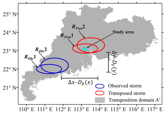
Figure 1.
Schematic diagram of rainfall spatial transposition of RainyDay. Where RObs1 and RObs2 are the observed rainfall events in the transposition domain, respectively; RTran1 and RTran2 are the rainfall events after transposition, respectively.
Step 1. Selecting the transposition domain. RainyDay requires that (i) the selected transposition domain should contain the study area; (ii) the selected transposition domain has the same climatic conditions and similar rainfall characteristics as the study area; (iii) the area of the transposition domain is more than 10 times larger than the study area. We selected a typical residential district in Guangzhou as case-study area. Following the requirements of RainyDay, Guangdong Province, which belongs to the same administrative region as the case-study area, is selected as the transposition domain.
Step 2. Identifying the “parent storms”. RainyDay selects the m largest t-hour rainfall events that occurred in the transposition domain over n-year record of gridded rainfall dataset, in terms of rainfall accumulation with the same size (i.e., single grid in this study) of study area. The selected rainfall events, which do not occur in the same 24 h, are temporally non-overlapping. That is, RainyDay only selects one t-hour event when there are two or more t-hour events in the top m events occurring in the same 24 h. These selected rainfall events are defined as “parent storms”.
Step 3. Calculating the distribution probability of extreme rainfall events. The occurred probability of extreme rainfall events is spatially non-uniform in the transposition domain. RainyDay calculates the probability through the two-dimensional Gaussian kernel according to the storm centers of the “parent storms”. The sum of the probability of each grid in the transposition domain is on one.
Step 4. Transposing rainfall events. RainyDay randomly selects k rainfall events from the “parent storms” to generate rainfall events, where k is an integer and indicates a “number of storms per year”. Besides, RainyDay assumes that k follows a Poisson distribution with annual occurrence rate , where represents the ratio of the selected m parent storms to n-year rainfall records, . More details about Poisson-distributed storm occurrences can be found in Wilson and Foufoula-Georgiou [49]. The selected rainfall events can be transposed to any position in the transposition domain according to the distribution probability of extreme rainfall events, but only the rainfall that occurred in the study area is calculated. RainyDay extracts the t-hour maximum rainfall, and the extracted rainfall is regarded as the maximum t-hour annual rainfall.
Step 5. Generating Tmax annual maximum rainfall. The Tmax annual maximum rainfall can be generated through repeating Step 4 Tmax times. To obtain the intensity-duration-frequency relationships, the maximas are ranked from smallest to largest based on rainfall accumulation. Then, the return period P of each these ranks can be calculated as . Each return period includes N realizations after repeating Step 4 and this step N times, that is, RainyDay provides the ensemble spread of rainfall accumulation rather than a single estimated value at each return period.
In this study, RainyDay is used to generate 5- to 100-yr design rainfall events with durations of 2 h, 6 h, 12 h and 24 h, respectively. Each return period includes 20 realizations for different durations. For simplicity, we only analyze the mean, minimum, and maximum of 20 realizations, since these results include the ensemble spread of all the realizations. In addition, we compare these results (i.e., RainyDay-based estimates) with IDF formula-based estimates to reflect the reasonability of the proposed framework.
2.2. Constructing Different Rainfall Scenarios
The design rainfall used in urban drainage systems and flood control is often calculated through coupling the IDF formula and the Chicago rainfall pattern [50]. To be consistent with this, the Chicago rainfall pattern is also used to allocate the RainyDay-based estimates at different times. The difference between IDF formula-based and the minimum, maximum and mean in 20 realizations of RainyDay-based estimates are compared. IDF formula is the empirical formula , where (L/(s·hm2)) indicates the design rainstorm intensity of t-minute duration at return period P (year); A, C, b, and n are the constant parameters that are derived and modified based on long-term rainfall records using the Gauss–Newton iterative algorithm [46]. For the case-study area, the IDF formula is shown in Equation (4).
In order to analyze the difference between the IDF-based and RainyDay-based estimates impact in urban flood analysis, we combine different return periods (5-, 10-, 20-, 50-, 100-yr), durations (2 h, 6 h, 12 h, 24 h), and estimates (IDF formula-based estimates, and the minimum, maximum, and mean in 20 realizations of RainyDay-based estimates) to generate 80 rainfall scenarios for urban flood analysis. For all rainfall scenarios, the rain peak coefficient is set to 0.375 to be consistent with the design specification for outdoor drainage in China [46].
2.3. Urban Hydrologic Model
In this study, an urban hydrologic model named SWMM is used to simulate and reflect the relationships between rainfall and runoff. SWMM is widely used in urban flood analysis and hydraulic practices, and it has very good simulated performances in both urban and natural basins [51,52]. Since the theory of the SWMM model is introduced in detail in a previous study by Gironás et al. [53], we do not show more details about the SWMM model in this study.
Because the calibrated and verified hydrological model in Zhu et al. [15] is used in this study, the reader is directed to Zhu et al. [15] for more information about case-study area and the performance of the model. In this model, the nonlinear reservoir method is selected to calculate the surface runoff, the Saint-Venant equations are used to calculate the flow, the Horton model is used to calculate the infiltration process, the Manning formula and the approximate continuity equation are used to convert the runoff of each sub basin into the outflow process, and the Newton-Raphson method and finite difference method are used to calculate the time-varying process of runoff. Zhu et al. [54] calibrated and verified the model based on the observed rainfall and runoff data, while the Nash-Sutcliffe efficiency (NSE) index is used to assess the model’s performance.
In order to reflect the performance of RainyDay-based estimates for runoff process simulation, we take the time distributions of the RainyDay-based and IDF formula-based estimates as the inputs of the constructed urban hydrologic model and compare their differences. The model used in this study is same as that in Zhu et al. [54] and the calibration and verification results show that the model can be used to simulate the runoff process of the case-study area. The applicability and rationality of the model are demonstrated. More details about the model can be found in Zhu et al. [54].
2.4. Projection Pursuit Algorithm
The projection pursuit algorithm is a robust and powerful algorithm for the exploratory analysis of multivariate high-dimensional data. It is widely used to reduce dimensionality for feature extraction, especially for flood and environment analysis. For instance, Zhi et al. [55] coupled the drainage model, 2D flood simulation model, and projection pursuit algorithm to assess urban flood risk; when Guo et al. [56] proposed an evaluation framework to assess atmospheric environment carrying capacity based on an evaluation index system including 20 indicators, the projection pursuit algorithm was used to reduce dimensionality. The basic theory of the projection pursuit algorithm is to project the data into low-dimensional subspace via projection vectors. It has the advantages of a strong anti-jamming capability and not depending on subjective evaluation criteria. In this study, the projection pursuit algorithm is adopted to analyze the comprehensive characteristics of urban flooding by constructing an evaluation index system. The system includes three indicators, i.e., flood time, maximum rate, and total inundation volume. Zhu et al. [40] demonstrated that flood characteristics could be estimated well based on these indicators. The general steps are summarized as follows; more details are provided in Kruskal and Shepard [57] and Zhu et al. [40].
Step 1: Construct and normalize the evaluation indicator set. Flood time, maximum rate, and total inundation volume are selected as the evaluation indicator set (X = {Xij|i = 1, 2, 3; j = 1, 2, …, p}), where Xij represents the value of the ith evaluation indicator of the jth sample, j and i represent the number of evaluation indicators and sample size, respectively. The normalized set is calculated as follow:
where Xjmax and Xjmin denote the maximum and minimum of ith evaluation indicator.
Step 2: Establishing the projection indicator function Q(a). The evaluation indicator set is synthesized into a 1 × 3 vector (i.e., ) as the projection direction. Therefore, the projection value of jth sample is calculated as follow:
Then, Q(a) can be expressed as:
where and note the interclass distance and local density of , respectively; represents the mean of ; means the cutoff radius; is the unit step function, if , ; otherwise, .
Step 3: Calculating the best projection direction. is determined by the projection direction if the value of the evaluation indicator is given. For the projection direction, the higher the value of the better. When the value of is at its maximum, the corresponding projection direction is the best. In order to seek the best projection direction, the optimum objective function can be constructed as max(), and the constraint condition is . Seeking the best projection direction is a nonlinear global optimization problem; the particle swarm optimization (PSO) technique is widely used to solve such problems. We also adopt it in this study, and more details are directed to Kennedy and Eberhart [58].
Step 4: Analyzing the comprehensive characteristics of urban flooding. The best projection values can be obtained through putting the best projections direction into Equation (4). The best projection values represent the comprehensive characteristics of urban flooding. The larger the values are, the more severe is the urban flood.
Based on analyzing the runoff processes at the outlet of the case-study area, we focus on the flood characteristics under RainyDay-based and IDF formula-based estimates at the manholes (i.e., junctions) for the case-study area drainage system in this section. Three flood indicators (i.e., flood time, maximum rate, total inundation volume), which are demonstrated to reflect the urban flood characteristics by Zhu et al. [40], are selected to analyze the flood characteristics at each manhole. The comprehensive flood characteristics are analyzed by combining these three indicators with the projection pursuit algorithm.
3. Data and Case-Study Area
3.1. Data
The hourly, 0.1° gauge-adjusted remotely sensed rainfall data (http://www.cma.gov.cn/2011qxfw/2011qsjgx/, accessed date: 15 November 2020) from the China Meteorological Administration merges CMORPH (the Climate Prediction Center Morphing algorithm) and the observations of 30,000 automatic rain gauges. This rainfall product is optimized and verified by the probability density function matching technique and optimal interpolation method. The temporal resolution is coarsened to one hour. Its total error is less than 10%, and the errors for heavy rainfall in the area with sparse ground gauge networks are less than 20%. The accuracy is higher than similar rainfall products and the product has been widely used for precipitation studies [59]. In order to verify the feasibility of estimating the design rainfall based on short-record remote sensing rainfall data, the rainfall data from 2008 to 2016 are selected in this study, where 2008 is the earliest year when data are available.
The rainfall and runoff data used for calibration and verification are observed from the case-study area, where the rainfall data is observed by RainLoggerTM rain gauge (RainWise Inc.; USA), and the runoff data is observed by Stingray open channel gauge (Greyline Instruments Inc.; Germany). The observed time steps are 10 min.
3.2. Case-Study Area
In this study, the transposition domain selected for RainyDay is Guangdong Province in the south of China. The latitude ranges from 20.08 to 25.32 °N, and longitude ranges from 109.04 to 117.20 °E (Figure 2). The area belongs to a subtropical monsoon climate, and the rainfall has the characteristics of large amount and high intensity. The annual average rainfall is 1300 to 2500 mm. The rainfall in this area is seasonal, mainly from April to September, and record-breaking rainfall and flood disasters occur frequently during these months.
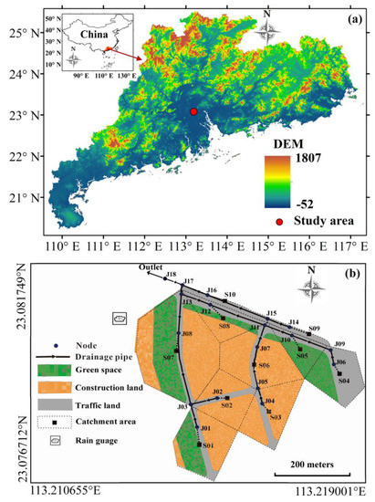
Figure 2.
The transposition domain and the location of the case-study area (a), and the land use and drainage system of the case-study area (b).
In order to verify the rationality of the proposed framework, a highly developed and typical residential area (22.08–23.09 °N, 113.20–113.21 °E) is selected as the case-study area in Guangzhou city (Figure 2). It belongs to the subtropical monsoon climate, and the average annual rainfall is 1675 mm. Extreme rainfall events may occur throughout the year, but are mainly concentrated in April to September. In the past 60 years, the maximum and minimum annual rainfall are 2865 and 1009 mm, respectively. The area of the case-study area is about 1.55 × 10⁵ m2, and its land use types can be generalized into three types such as building, green space, and road land (Figure 2). The slope ratio of the drainage system is 0.1~1.0%, and the pipe diameter is 600~1650 mm. The drainage system of the case-study area is designed according to rainfall accumulation at 2-yr return period. However, the regional flood problem has become increasingly prominent with increasing record-breaking extreme rainfall events.
According to the generalization theory of SWMM, the case-study area is divided into 10 sub-catchments, while the drainage system is generalized into 18 pipes, 18 manholes, and 1 outlet (Figure 2). More details are referred to in Zhu et al. [54].
4. Results
4.1. Estimating the Design Rainfall
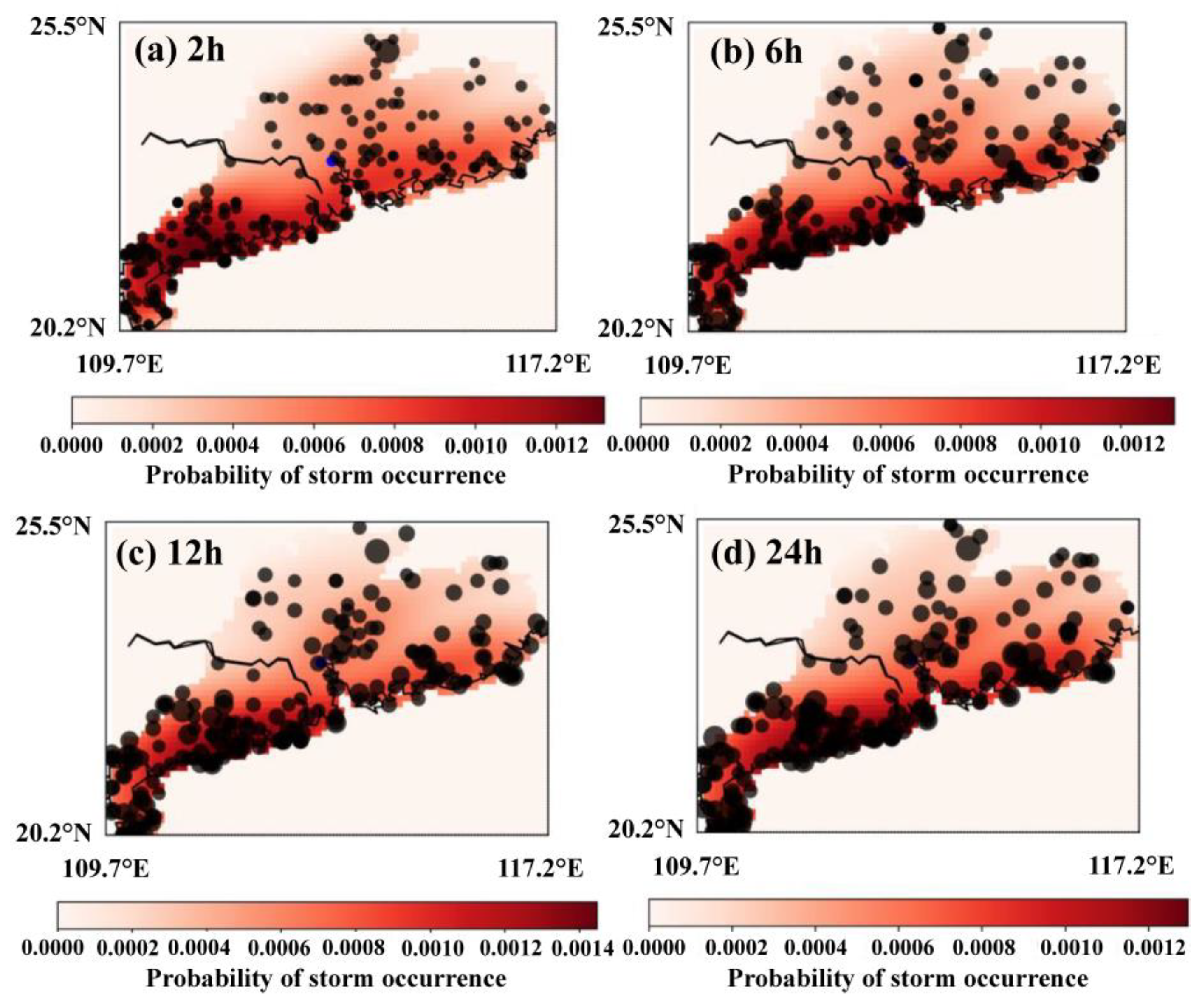
The important assumption of RainyDay for estimating design rainfall is that the storms in the transition domain are likely to occur in the study area. In order to illustrate the rationality of the selected transition domain, this study analyzes the spatial distribution and storm occurrence probability of 200 maximum storms under different durations (2 h, 6 h, 12 h, and 24 h) (Figure 3). The spatial distribution of storms with different durations is basically similar to each other. Generally speaking, the frequency of storms in coastal areas is relatively higher, but its spatial distribution is still relatively random, that is, heavy storms may occur everywhere in the selected transition domain (Figure 3). Similar to the spatial distribution, the spatial probability distribution of storms in the transition domain is relatively uniform, but there are still some differences. The storm occurrence probability decreases from south to north (Figure 3), which is in line with the actual distribution of storms (see Wang et al. [60] for evaluation of rainfall distribution in different precipitation products). The selected transition domain is reasonable since the probability of storm occurrence of 200 maximum storms varies from around 0.0002 to 0.0014 in the transition domain, i.e., the storms in the transition domain are likely to occur in the study area or other regions.
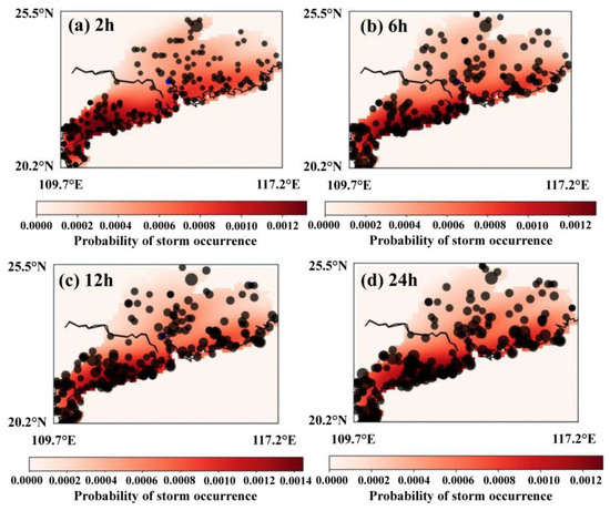
Figure 3.
The probability of storm occurrence and spatial distribution of 200 maximum storms under 2 h (a), 6 h (b), 12 h (c), and 24 h (d) durations over the transition domain. Shading denotes spatial probability of storm occurrence calculated based on 200 maximum storms. Black dots represent the rainfall centroids of 200 maximum storms, and its size means the relative rainfall depth of each storm.
Figure 4 shows the relationships between IDF formula-based and RainyDay-based estimates for different durations at different return periods. The ensemble spread of 20 realizations is shown as shaded area. Comparing results indicates that RainyDay is generally able to estimate urban extreme rainfall for different durations, but it may relatively underestimate or overestimate the rainfall accumulation. The results show that RainyDay usually underestimates the rainfall accumulation at low return periods or short rainfall durations; the RainyDay-based estimates are usually larger than the IDF formula-based estimates when the rainfall duration is long or the return period is high. Specifically, RainyDay overall underestimates the rainfall accumulation when the rainfall duration is 2 h at different return periods. The degree of underestimation, which varies from 0.4% (100-yr) to 57% (5-yr), decreases with increasing the return period (Table 1). When the duration reaches 6 h, the underestimation is improved. The IDF formula-based estimates, overall, fall within the ensemble spread of RainyDay-based estimates with the increase of duration. At each return period for 6 h or longer durations, the absolute value of the ratio of at least one RainyDay-based estimate (maximum, minimum, or average estimates) to IDF formula-based estimate is less than 10% (Table 1).
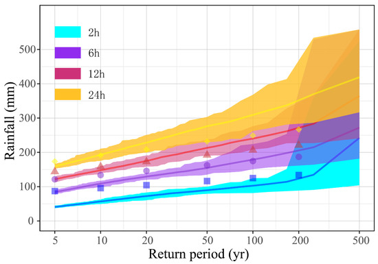
Figure 4.
The relationships between IDF formula-based and RainyDay-based estimates for different durations at different return periods. The shaded areas mean the ensemble spread of RainyDay-based estimates. The solid lines denote the ensemble mean for 20 realizations. The symbols of different shapes represent the IDF formula-based estimates.

Table 1.
Relative deviations between IDF formula-based and RainyDay-based estimates (%).
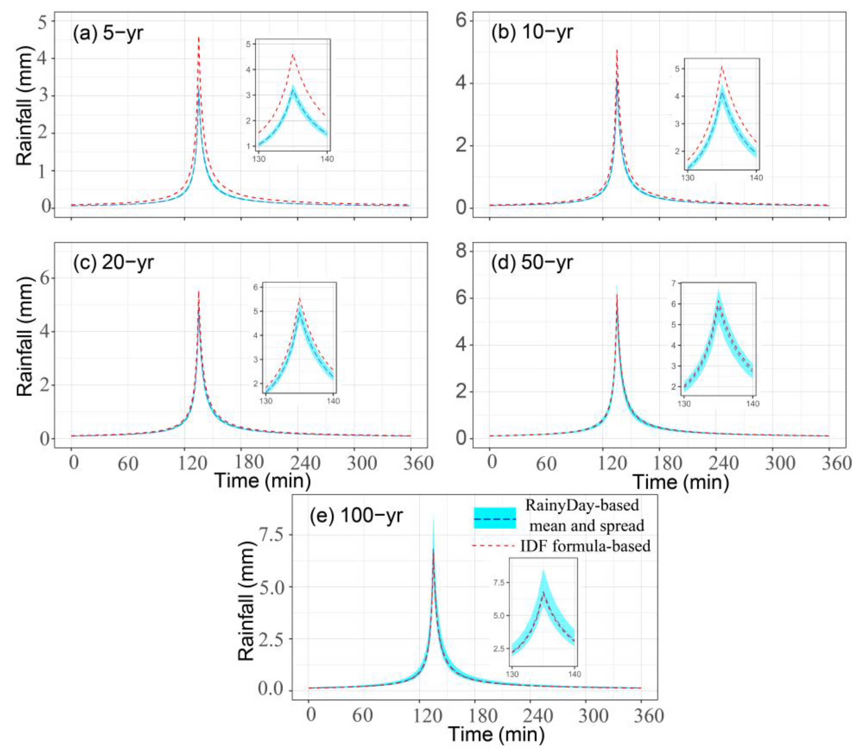
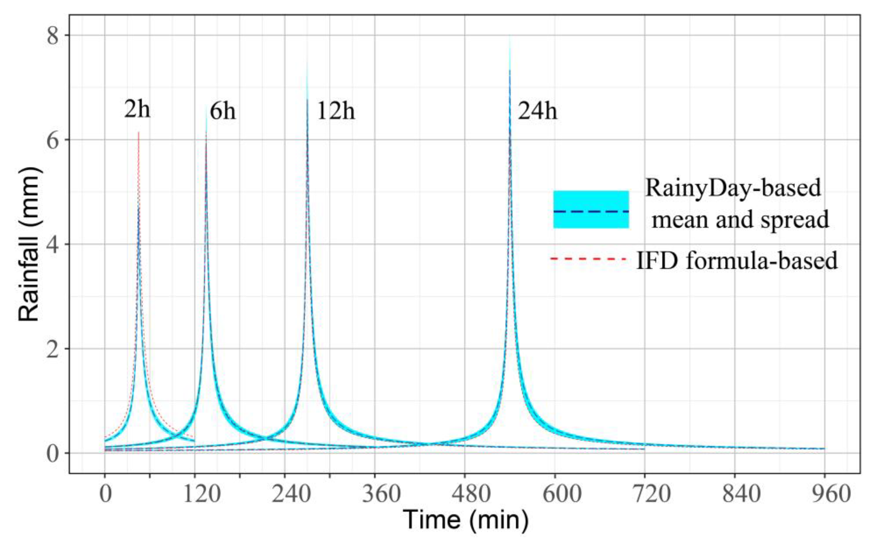
The IDF formula-based estimates gradually approach to the lower boundary of the shaded area with increasing return period. It indicates that the RainyDay-based estimates basically can reflect the observed design rainfall for long (6 h or longer) durations. To be consistent with the design specification for outdoor drainage in China, the time distributions of the RainyDay-based and IDF formula-based estimates for urban flood simulation are determined by the Chicago rainfall pattern. The time distribution results show that the main difference comes from the rainfall peak. The rainfall peak is underestimated from RainyDay-based estimates at low return periods or short rainfall durations, while it is generally matched or slightly overestimated at high return periods or for long rainfall duration. In order to better explain this fact, the time distributions at different return periods for 6 h duration and at 20-yr return period for different durations are selected as in the below examples (Figure 5 and Figure 6). When the duration is 6 h, the rainfall peak of the RainyDay-based estimates is relatively smaller than the IDF formula-based estimates at 5- and 10-yr return period, but the rainfall peak of IDF formula-based estimates generally falls within the ensemble spread of RainyDay-based estimates, and the average of the ensemble spread is generally matched to the IDF formula-based estimates when the return period reaches 50-yr or higher (Figure 5). On the other hand, when the return period is at 20-yr return period, the time distributions of RainyDay-based and IDF formula-based estimates are essentially coincidental, and the coincidence increases with lengthening rainfall duration (Figure 6). Overall, the RainyDay-based estimates show a good performance for design rainfall analysis. The relationship between the time distributions of RainyDay-based and IDF formula-based estimates at other return periods for other rainfall durations are similar to the above selected rainfall scenarios, so the time distributions of other scenarios are not shown.

Figure 5.
The time distributions of RainyDay-based and IDF formula-based estimates at 5-yr (a), 10-yr (b), 20-yr (c), 50-yr (d), and 100-yr (e) return periods for 6 h duration.

Figure 6.
The time distributions of RainyDay-based and IDF formula-based estimates at 20-yr return period for different durations.
4.2. Simulating the Runoff Process Based on RainyDay-Based Estimates
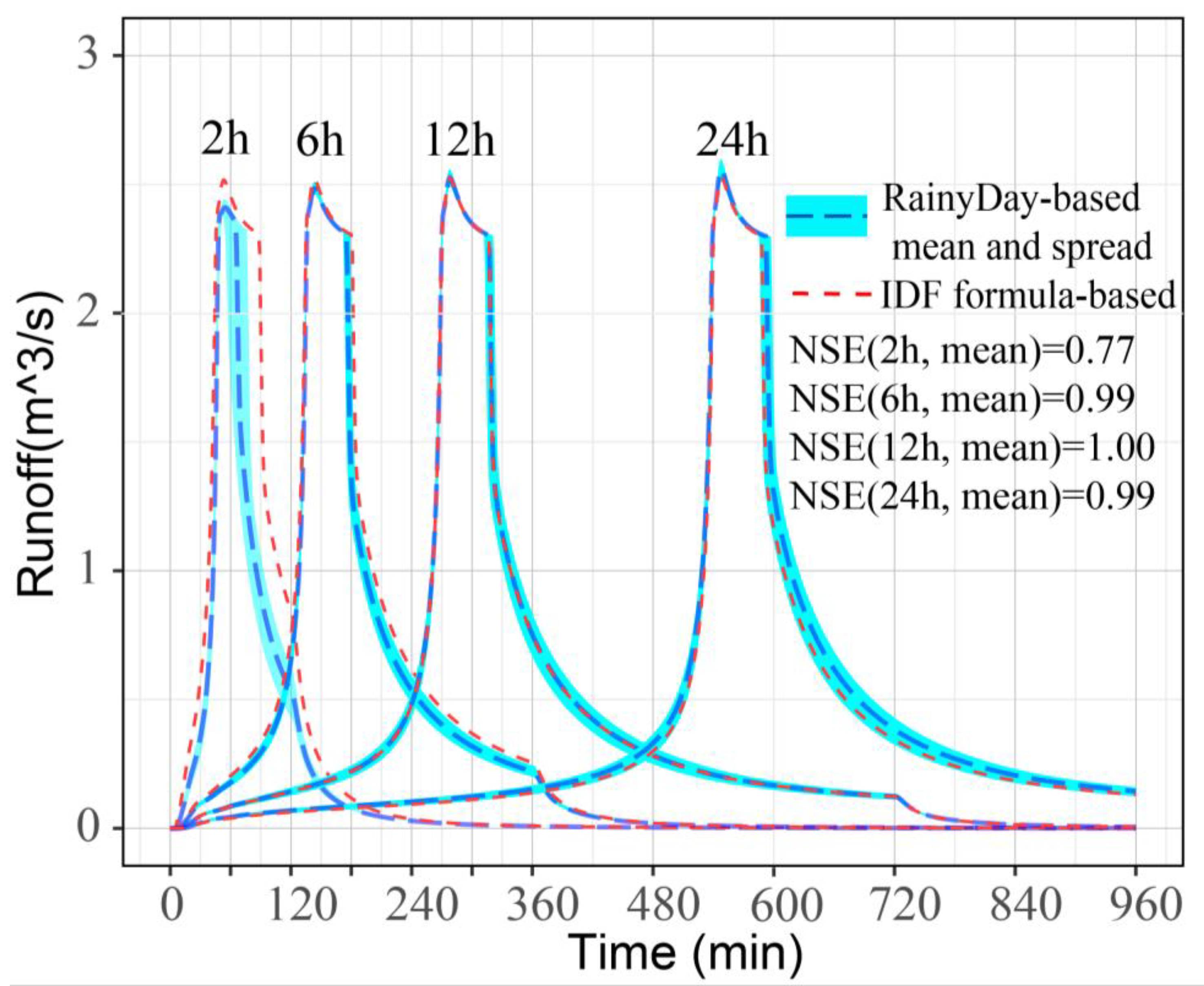
The simulated results show that the RaiyDay-based estimates basically can be used for runoff process simulation. The difference between the runoff processes of RainyDay-based and IDF formula-based estimates is similar to the time distributions of design rainfall, but the difference of peak discharge is smaller than the rainfall peak. Similar to the analysis of time distribution of rainfall estimates, we also take the runoff processes at different return periods for 6 h duration and at 20-yr return period for different durations as in the below example (Figure 7 and Figure 8). The runoff processes of RainyDay-based and IDF formula-based estimates indicate that the difference of runoff process decreases as the rainfall duration lengthens. The difference of peak discharge at high return periods (20-yr or higher) or for long durations (6 h or longer) is very small. For example, the difference of the RainyDay-based and IDF formula-based rainfall peaks is relatively significant, but the differences of peak discharges are very small at 5- and 10-yr return periods (Figure 5 and Figure 7). The RainyDay-based peak discharges become closer and closer, and even approximate overlapping IDF formula-based peak discharges with increasing return period. For the same return period (take 20-yr return period for example), the peak discharge is still slightly underestimated for 2 h duration, but the runoff process is predicted pretty well with the lengthening duration (Figure 8). In addition, we use NSE to evaluate the predicted performance of RainyDay-based estimates, i.e., the difference of runoff processes between RainyDay-based and IDF formula-based estimates. Results show that the values of NSE are generally small for short duration or at low return period (e.g., NSE = 0.53 at 5-yr return period for 6 h duration, NSE = 0.77 at 20-yr return period for 2 h duration); however, the values become larger with increasing rainfall duration or rainfall return period (e.g., NSE = 0.98 at 100-yr return period for 6 h duration, NSE = 0.99 at 20-yr return period for 24 h duration). For long duration (6 h or longer) or high return period (10-yr or higher), the values of NSE are generally above 0.5, i.e., the RainyDay-based estimates of long duration or high return period are satisfied to analyze the runoff process.
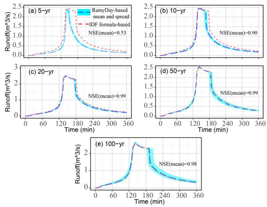
Figure 7.
The runoff processes at the outlet of the case-study area at 5-yr (a), 10-yr (b), 20-yr (c), 50-yr (d), and 100-yr (e) return periods for 6 h duration.

Figure 8.
The runoff processes at the outlet of the case-study area at 20-yr return period for different durations.
4.3. Analyzing Flood Characteristics Based on RainyDay-Based Estimates
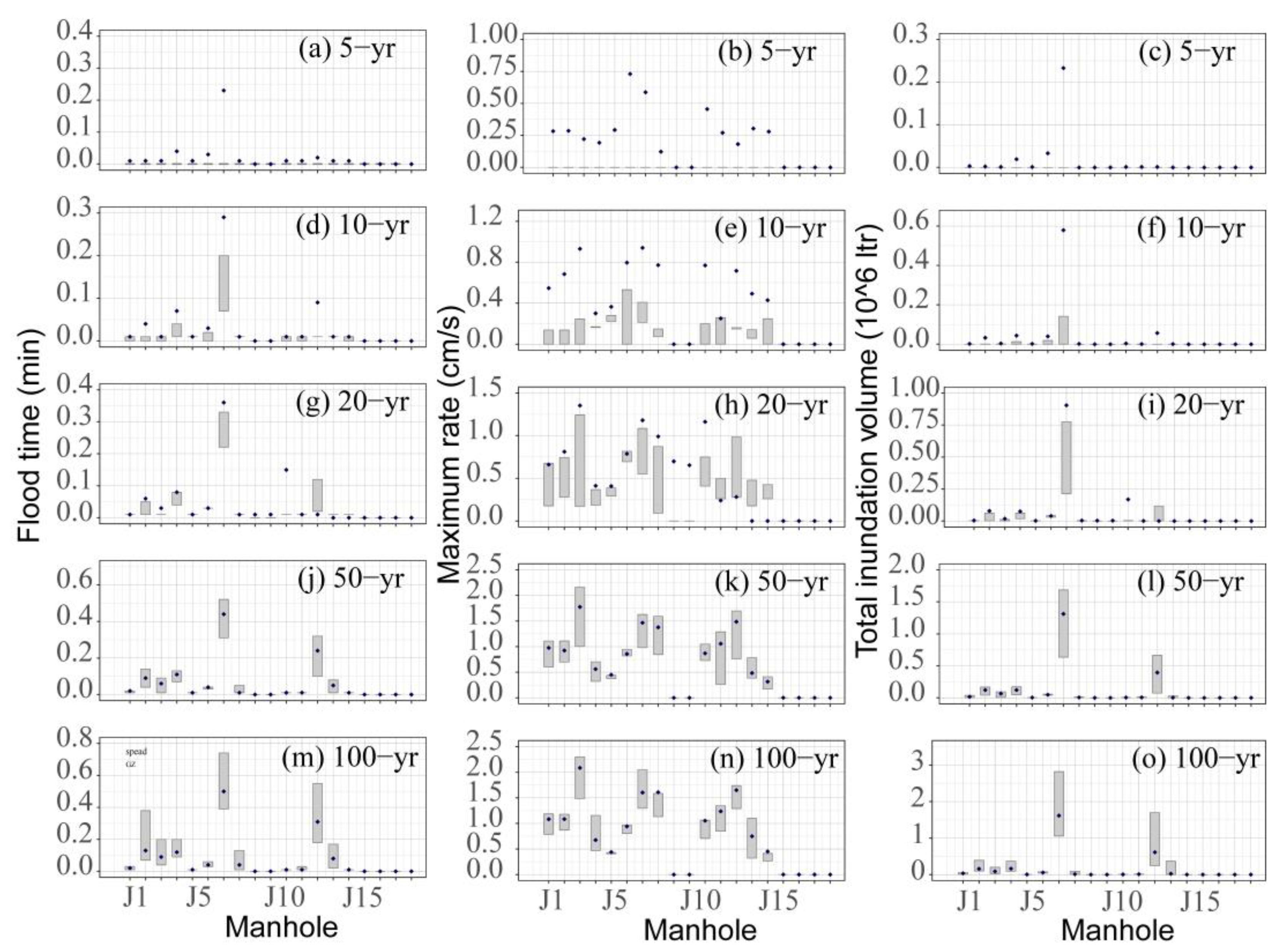
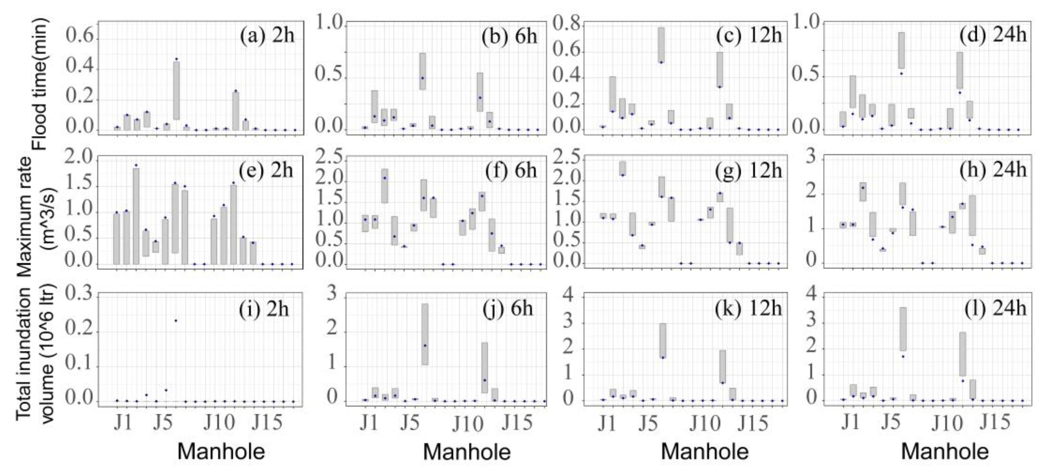
Results show that the characteristics of urban flooding are generally underestimated based on RainyDay-based estimates at low return periods or short rainfall durations. For short durations or at low return periods, the underestimation of the values of these indicators at each manhole are more significant than runoff processes at the outlet. Specifically, the RainyDay-based estimates underestimate the values of flood time, maximum rate, and total inundation volume when the return period is lower than 10-yr or duration is shorter than 6 h. The underestimation decreases with increasing return period or lengthening rainfall duration. The values of flood time, maximum rate, and total inundation volume simulated based on IDF formula-based estimates generally fall within the ensemble spread of RainyDay-based estimates at high (20-yr or high) return period or long (6 h or longer) duration (Figure 9 and Figure 10). That is to say, the RainyDay-based estimates can be used to assess the flood characteristics at each manhole at relatively high return periods or long rainfall durations.

Figure 9.
The flood characteristics of each manhole at different return periods for 6 h duration. The flood time at 5-yr, 10-yr, 20-yr, 50-yr, and 100-yr return periods is shown in (a), (d), (g), (j), and (m), respectively. The maximum rate at 5-yr, 10-yr, 20-yr, 50-yr, and 100-yr return periods is shown in (b), (e), (h), (k), and (n), respectively. The total inundation volume at 5-yr, 10-yr, 20-yr, 50-yr, and 100-yr return periods is shown in (c), (f), (i), (l), and (o), respectively. The grey boxes indicate the spread of RainyDay-based, and points represent IDF formula-based, values.

Figure 10.
The flood characteristics of each manhole at 20-yr return period for different durations. The flood time for 2 h, 6 h, 12 h, and 24 h durations is shown in (a–d), respectively. The maximum rate for 2 h, 6 h, 12 h, and 24 h durations is shown in (e–h), respectively. The total inundation volume for 2 h, 6 h, 12 h, and 24 h durations is shown in (i–l), respectively. The grey boxes indicate the spread of RainyDay-based, and points represent IDF formula-based, values.
In order to better clarify the changing characteristics of urban flooding at each manhole with rainfall return period or rainfall duration, we also take the flood characteristics of each manhole at 20-yr return period for different durations and at different return periods for 6 h duration as an example. For 6 h rainfall duration, the RainyDay-based estimates significantly underestimate the values of the selected indicators at 5-yr return period; when the return period increases to 10-yr, the RainyDay-based estimates can reflect the flood characteristics at each manhole to a certain extent, but it is still relatively underestimated; while the rainfall return period reaches 20-yr or more, the values of indicators simulated by IDF formula-based estimates basically fall within the ensemble spread of RainyDay-based estimates. On the other hand, when the rainfall return period is 20-yr, the RainyDay-based estimates can basically reflect the flood characteristics of each manhole under different rainfall duration scenarios, especially for long (6 h or longer) rainfall duration. The flood characteristics of some manholes will be slightly overestimated with the increasing rainfall duration.
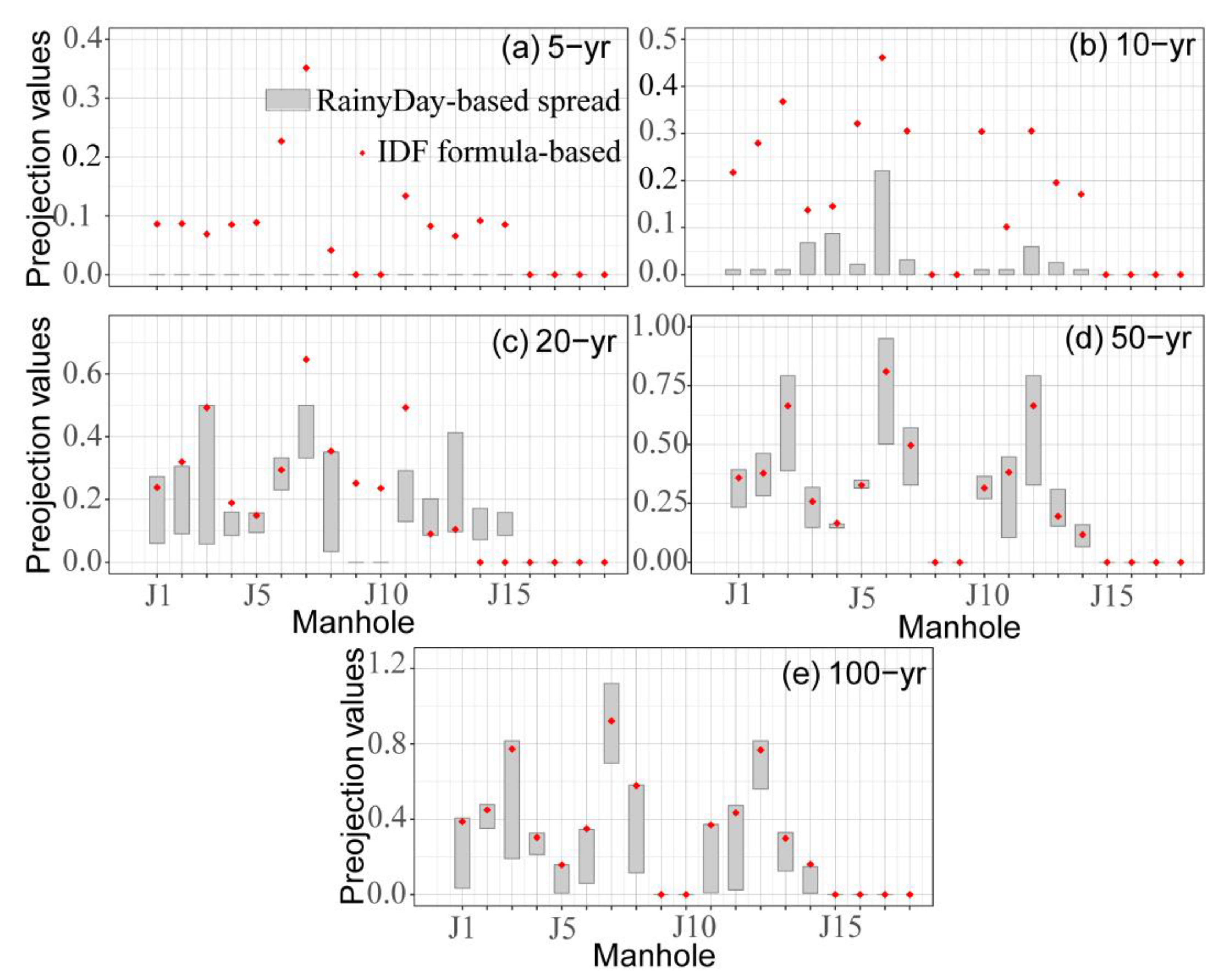
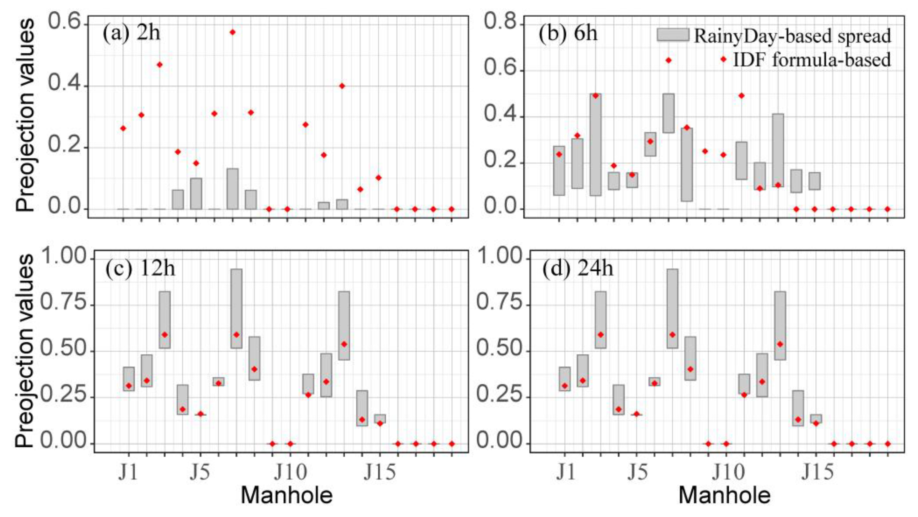
The results shown in Figure 9 and Figure 10 cannot comprehensively assess the flood characteristics of each manhole, therefore, the projection pursuit algorithm is used to reduce three dimensions (i.e., three indicators) to one dimension. The one-dimension values (i.e., the projection values) indicate the comprehensive characteristics of urban flooding for each manhole. Results show that the flood hotspot manholes are J3, J7, and J13, but they are significant underestimated based on RainyDay-based estimates at low return periods or short rainfall durations (Figure 9 and Figure 10). The changing characteristics of projection values with return periods or duration are similar to the values of the three indicators, but the degree of underestimation for the projection values is larger than the values of indicators (Figure 11 and Figure 12). However, the degree of underestimation decreases with increasing return period or duration. Similar to the values of three indicators, the projection values estimated based on IDF formula-based estimates fall within the RainyDay-based ensemble spread at high (20-yr or higher) return periods or long (6 h or longer) durations. The comprehensive analysis results for urban flooding demonstrates that the RainyDay-based estimates can be used for urban flood analysis, especially for high (20-yr or high) return periods or long (6 h or longer) durations.
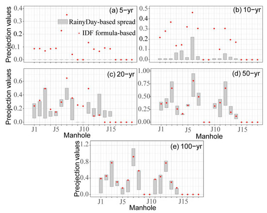
Figure 11.
The projection values of each manhole at 5-yr (a), 10-yr (b), 20-yr (c), 50-yr (d), and 100-yr (e) return periods for 6 h duration.

Figure 12.
The projection values of each manhole at 20-yr return period for 2 h (a), 6 h (b), 12 h (c), and 24 h (d) durations.
5. Discussion
Regarding the limitations of traditional urban flood analysis, lacking high-resolution rainfall records should be one of the primary issues [61]. Although many models and frameworks were proposed to solve this issue, many inherent limitations still exist [16,62]. Therefore, a modeling framework for urban flood analysis is introduced based on short-record rainfall from remote sensing, RainyDay, and urban hydrological model, which effectively overcomes the high-temporal-resolution and long-term rainfall requirements for urban flood analysis. It should be emphasized that this work does not seek to show the proposed framework better than the traditional methods, but rather to provide an alternative framework for urban flood analysis based on short-term remote sensing rainfall records, and discuss its feasibility and rationality.
The results of this study for design rainfall estimates are very similar to Wright et al. [27] , though simulated at a much smaller scale (0.155 km2 vs. 4000 km2) based on a different time-space resolution (hourly vs. hourly, and 3 h; 0.1° grid vs. 4-km, and 0.25° grid) and length of rainfall records (nine-year vs. 13-year, and 17-year). These two studies show that the design rainfall is generally underestimated with remote sensing data at low return periods or short durations. The underestimation could be explained by the length of rainfall records and spatial resolution (nine-year and 0.1° grid for the remote sensing rainfall record vs. more than 20 years and approximately 0.1 m2 for the rain gages) in this study. For short duration rainfall, temporal resampling using RainyDay is significantly affected by rainfall detection errors on bias correction and conditional biases [63,64,65,66]. Also, this can be attributed to the fundamental structure of RainyDay, i.e., the Poisson distribution is utilized in this study (see Kim and Onof [67] for discussion). Conversely, the slight overestimation of RainyDay-based estimates are showed at high return periods and long durations, but the overestimation is not as severely as the underestimation. This might potentially be attributed to conditional bias for rain rate [68] and the domain area including coastal areas where the typhoon landed. Some existed studies show that the accuracy of the estimates may be improved by higher temporal-spatial resolution remote sensing data, which can better address and understand some rainfall biases [27,69].
The main parts of this study include estimating design rainfall based on nine-year remote sensing rainfall and RainyDay, and revealing the relationship between design rainfall and runoff through hydrological model. Previous studies showed that the design rainfall can be well estimated by RainyDay at different scales (e.g., 14.3 km2 in Zhou et al. [70], 4400 km2 in Wright et al. [66]). Though the feasibility is shown varying from small to large scales, the limit on the size of study area can arise since the presence of complex terrain features. The reader is directed to Wright et al. [27] for more discussion. On the other hand, the selected hydrological model (i.e., SWMM) has been widely used for modeling rainfall-driven flood at different scales, especially for urban areas. The proposed modeling framework offers opportunities to analyze urban flooding based on short-record remote sensing rainfall and hydrologic model. However, the size of the case-study area is small, it may cannot represent all the urban flood conditions. We will continue to expand the capabilities of the proposed modeling framework.
Case study shows that the runoff process at the outlet of case-study area and the flood characteristics (i.e., flood time, maximum rate, total inundation volume) of each manhole can be simulated well at relatively high return periods (20-yr or higher) or long durations (6 h or longer) based on the selected rainfall record. But the flood characteristics are more sensitive to the return period and duration of design rainfall than runoff process. The main difference in the rainfall hydrographs between RainyDay-based and IDF formula-based is from the peak rainfall, which can significantly impact the flood characteristics.
Our findings indicate that the rainfall estimates play a key role in flood analysis, similar results are also showed in Peleg et al. [26]. That is, improving the accuracy of the rainfall estimates is the most important in the proposed framework. Lots of studies indicated that rainfall estimates based on historical rainfall records might not be appropriate due to climate change [71]. Doing so would require higher-resolution remote sensing rainfall data and considering climate change [27,70,71]. We are developing frameworks for considering both rainfall space-time structure and climate change based on Regional Climate Model (RCM) simulations for RainyDay-based rainfall estimates.
Despite the proposed framework overcomes some drawbacks (e.g., rainfall records) of traditional approaches for urban flood analysis, there still remain several limitations. (i) Applicability of the proposed framework is insufficient for low return period or short duration rainfall scenarios. The undervaluation of design rainfall and urban flood characteristics are generally showed at these scenarios. The main reason is mentioned above, and the applicability can be improved by utilizing higher resolution and longer rainfall records [70,72]. (ii) The uncertainties from the rainfall data and RainyDay are hard to minimize, which have direct impacts in design rainfall estimates and urban flood analysis. The dominant uncertainty in the input rainfall data comes from the difference between remote sensing rainfall data and ground-based observations [27,73]; and the uncertainty in Rainyday comes from the input requirements (e.g., geographic transposition domain, rainfall record) and its structure [70]. (iii) The proposed framework uses idealized assumption (i.e., Chicago rainfall pattern) to determine the distributions of design rainfall. That is consistent with the guidelines of design rainfall [46]. On the other hand, the rainfall temporal resolution of remote sensing records is general coarser than 30-min. Comparing the relationships between RainyDay-based and IDF formula-based analysis results suggest that the proposed framework is an applicable way for analyzing urban flooding at high return periods (20-yr or higher) or long durations (6 h or longer). Though limitations still remain, we continue to develop its capabilities.
6. Conclusions
Rainfall remote sensing datasets have the advantages of high temporal-spatial resolution and large coverage, which can overcome limitations such as a lack of gauge-based rainfall records. In this study, we propose a modeling framework for urban flood analysis based on short-record remote sensing rainfall and hydrologic model. The framework is largely motivated by the fact that, in spite of increased interest in urban flood analysis using high-temporal remote sensing rainfall data, the inherent limitation of a lack of long-term high-temporal rainfall data still exists. We used RainyDay and a nine-year record of hourly, 0.1° remotely sensed rainfall data to generate extreme rainfall events for an urban hydrologic model (SWMM). The rainfall estimates of RainyDay-based and IDF formula-based methods were compared, as well as the corresponding runoff process at 5-, 10-, 20-, 50-, 100-yr return periods for 2 h, 6 h, 12 h, and 24 h durations. In addition, the projection pursuit method was used to reflect the comprehensive characteristics of the urban flooding. A typical urban drainage basin in the south of China was selected as the case-study area. The main conclusions include the following:
- Combining RainyDay and short-term remotely sensed rainfall data can lengthen the rainfall record through transposing the spatial location of observed rainfall events. It is able to estimate urban extreme rainfall at different return periods (e.g., range in return period from 5- to 100-yr), despite the short (nine-year) observed rainfall record. According to a comparison of the differences between the RainyDay-based and IDF formula-based (a traditional published source of rainfall frequencies) rainfall estimates, RainyDay-based rainfall estimates are basically acceptable for estimating regional design rainfall, especially for relatively high return periods (20-yr or higher) or long durations (6 h or longer).
- The proposed framework shows a good performance for runoff process simulation at the outlet based on RainyDay-based estimates, especially for high return periods or long durations. In the case study, the difference of runoff process between RainyDay-based and IDF formula-based methods is relatively significant at low return periods or for short durations (e.g., NSE = 0.53 at 5-yr return period for 6 h duration), but the difference decreases with the lengthening rainfall duration or increasing return period. The values of NSE are generally above 0.90 at high return periods or long durations.
- Contrasting with the flood-simulated results under different return periods and durations, the flood characteristics of urban flooding at each manhole can be generally revealed based on RainyDay-based estimates at relatively high (20-yr and beyond) return periods or long (6 h or longer) durations. Similar to the results of runoff processes, though RainyDay-based estimates basically underestimate the values of flood indicators (i.e., flood time, maximum rainfall rate, total maximum rainfall volume) or the comprehensive characteristics of urban flooding under low return period or short duration scenarios, these values can be well revealed with increasing duration or return period.
- The proposed modeling framework provides an alternative framework for urban flood analysis in an ungauged drainage basin. This alternative is attractive for the following reasons. First, the proposed framework can produce probabilistic extreme rainfall scenarios based on a very short rainfall record (e.g., nine-year in this study), and it excludes the older rainfall records to eliminate the effect of nonstationarity. Second, the proposed framework provides a way to estimate the ensemble spread of rainfall and flood estimates, rather than a single estimate value; such spread is central to hydrological engineering practices.
Author Contributions
Conceptualization, Z.Z. and Y.C.; methodology, Z.Z. and Y.Y.; software, Z.Z. and Y.Y.; validation, Z.Z., Y.C., and Z.Y.; investigation, Z.Z.; resources, Y.C. and Z.Y.; writing—original draft preparation, Z.Z. and Y.Y.; writing—review and editing, Y.C. and Z.Z.; visualization, Z.Z. and Y.Y.; supervision, Z.Y.; funding acquisition, Z.Y. and Z.Z. All authors have read and agreed to the published version of the manuscript.
Funding
This research was funded by the Local Innovative and Research Teams Project of Guangdong Pearl River Talents Program (2017BT01Z176), Key Special Project for Introduced Talents Team of Southern Marine Science and Engineering Guangdong Laboratory (Guangzhou) (GML2019ZD0403), and National Natural Science Foundation of China (52009021).
Institutional Review Board Statement
Not applicable.
Informed Consent Statement
Not applicable.
Data Availability Statement
The data that support the findings of this study are available from the corresponding author upon reasonable request.
Acknowledgments
The authors wish to express their gratitude to all authors of the numerous technical reports used for this paper. We would also like to thank the editor as well as the reviewers whose constructive criticism contributed greatly to this paper.
Conflicts of Interest
The authors declare no conflict of interest.
References
- Fowler, H.J.; Lenderink, G.; Prein, A.F.; Westra, S.; Allan, R.P.; Ban, N.; Barbero, R.; Berg, P.; Blenkinsop, S.; Do, H.X.; et al. Anthropogenic Intensification of Short-Duration Rainfall Extremes. Nat. Rev. Earth Environ. 2021, 2, 107–122. [Google Scholar] [CrossRef]
- Liu, B.; Tan, X.; Gan, T.Y.; Chen, X.; Lin, K.; Lu, M.; Liu, Z. Global Atmospheric Moisture Transport Associated with Precipitation Extremes: Mechanisms and Climate Change Impacts. WIREs Water 2020, 7, e1412. [Google Scholar] [CrossRef]
- Kemter, M.; Merz, B.; Marwan, N.; Vorogushyn, S.; Blöschl, G. Joint Trends in Flood Magnitudes and Spatial Extents Across Europe. Geophys. Res. Lett. 2020, 46, e2020GL087464. [Google Scholar] [CrossRef]
- Wu, Z.; Zhou, Y.; Wang, H.; Jiang, Z. Depth Prediction of Urban Flood under Different Rainfall Return Periods Based on Deep Learning and Data Warehouse. Sci. Total Environ. 2020, 716, 137077. [Google Scholar] [CrossRef]
- World Resources Institute RELEASE. New Data Shows Millions of People, Trillions in Property at Risk from Flooding—But Infrastructure Investments Now Can Significantly Lower Flood Risk. Available online: https://www.wri.org/news/2020/04/release-new-data-shows-millions-people-trillions-property-risk-flooding-infrastructure (accessed on 13 April 2021).
- Du, S.; Scussolini, P.; Ward, P.J.; Zhang, M.; Wen, J.; Wang, L.; Koks, E.; Diaz-Loaiza, A.; Gao, J.; Ke, Q.; et al. Hard or Soft Flood Adaptation? Advantages of a Hybrid Strategy for Shanghai. Glob. Environ. Chang. 2020, 61, 102037. [Google Scholar] [CrossRef]
- Santos, P.P.; Pereira, S.; Zêzere, J.L.; Tavares, A.O.; Reis, E.; Garcia, R.A.C.; Oliveira, S.C. A Comprehensive Approach to Understanding Flood Risk Drivers at the Municipal Level. J. Environ. Manag. 2020, 260, 110127. [Google Scholar] [CrossRef] [PubMed]
- Chen, J.; Wang, Z.; Wu, X.; Lai, C.; Chen, X. Evaluation of TMPA 3B42-V7 Product on Extreme Precipitation Estimates. Remote Sens. 2021, 13, 209. [Google Scholar] [CrossRef]
- Najibi, N.; Devineni, N. Recent Trends in the Frequency and Duration of Global Floods. Earth Syst. Dyn. 2018, 9, 757–783. [Google Scholar] [CrossRef]
- Zhou, Z.; Smith, J.A.; Yang, L.; Baeck, M.L.; Chaney, M.; Ten Veldhuis, M.-C.; Deng, H.; Liu, S. The Complexities of Urban Flood Response: Flood Frequency Analyses for the Charlotte Metropolitan Region: The complexities of urban flood response. Water Resour. Res. 2017, 53, 7401–7425. [Google Scholar] [CrossRef]
- Zhu, Z.; Wright, D.B.; Yu, G. The Impact of Rainfall Space-Time Structure in Flood Frequency Analysis. Water Resour. Res. 2018, 54, 8983–8998. [Google Scholar] [CrossRef]
- Yu, G.; Wright, D.B.; Holman, K.D. Connecting Hydrometeorological Processes to Low-Probability Floods in the Mountainous Colorado Front Range. Water Resour. Res. 2021, 57, e2021WR029768. [Google Scholar] [CrossRef]
- Sun, Y.; Wendi, D.; Kim, D.E.; Liong, S.-Y. Deriving Intensity–Duration–Frequency (IDF) Curves Using Downscaled in Situ Rainfall Assimilated with Remote Sensing Data. Geosci. Lett. 2019, 6, 17. [Google Scholar] [CrossRef]
- Dai, Q.; Bray, M.; Zhuo, L.; Islam, T.; Han, D. A Scheme for Rain Gauge Network Design Based on Remotely Sensed Rainfall Measurements. J. Hydrometeorol. 2017, 18, 363–379. [Google Scholar] [CrossRef]
- Yu, G.; Wright, D.B.; Zhu, Z.; Smith, C.; Holman, K.D. Process-Based Flood Frequency Analysis in an Agricultural Watershed Exhibiting Nonstationary Flood Seasonality. Hydrol. Earth Syst. Sci. 2019, 23, 2225–2243. [Google Scholar] [CrossRef]
- Li, W.; Lin, K.; Zhao, T.; Lan, T.; Chen, X.; Du, H.; Chen, H. Risk Assessment and Sensitivity Analysis of Flash Floods in Ungauged Basins Using Coupled Hydrologic and Hydrodynamic Models. J. Hydrol. 2019, 572, 108–120. [Google Scholar] [CrossRef]
- Kastridis, A.; Kirkenidis, C.; Sapountzis, M. An Integrated Approach of Flash Flood Analysis in Ungauged Mediterranean Watersheds Using Post-Flood Surveys and Unmanned Aerial Vehicles. Hydrol. Process. 2020, 34, 4920–4939. [Google Scholar] [CrossRef]
- Papaioannou, G.; Vasiliades, L.; Loukas, A.; Aronica, G.T. Probabilistic Flood Inundation Mapping at Ungauged Streams Due to Roughness Coefficient Uncertainty in Hydraulic Modelling. Adv. Geosci. 2017, 44, 23–34. [Google Scholar] [CrossRef]
- Ghorbani, M.A.; Ruskeepää, H.; Singh, V.P.; Sivakumar, B. Flood Frequency Analysis Using Mathematica. Turk. J. Eng. Environ. Sci. 2010, 34, 171–188. [Google Scholar] [CrossRef]
- Salman, A.M.; Li, Y. Flood Risk Assessment, Future Trend Modeling, and Risk Communication: A Review of Ongoing Research. Nat. Hazards Rev. 2018, 19, 4018011. [Google Scholar] [CrossRef]
- François, B.; Schlef, K.E.; Wi, S.; Brown, C.M. Design Considerations for Riverine Floods in a Changing Climate—A Review. J. Hydrol. 2019, 574, 557–573. [Google Scholar] [CrossRef]
- Herman, M.R.; Nejadhashemi, A.P.; Abouali, M.; Hernandez-Suarez, J.S.; Daneshvar, F.; Zhang, Z.; Anderson, M.C.; Sadeghi, A.M.; Hain, C.R.; Sharifi, A. Evaluating the Role of Evapotranspiration Remote Sensing Data in Improving Hydrological Modeling Predictability. J. Hydrol. 2018, 556, 39–49. [Google Scholar] [CrossRef]
- Nguyen, H.D.; Fox, D.; Dang, D.K.; Pham, L.T.; Viet Du, Q.V.; Nguyen, T.H.T.; Dang, T.N.; Tran, V.T.; Vu, P.L.; Nguyen, Q.-H.; et al. Predicting Future Urban Flood Risk Using Land Change and Hydraulic Modeling in a River Watershed in the Central Province of Vietnam. Remote Sens. 2021, 13, 262. [Google Scholar] [CrossRef]
- Mohanty, M.P.; Sherly, M.A.; Karmakar, S.; Ghosh, S. Regionalized Design Rainfall Estimation: An Appraisal of Inundation Mapping for Flood Management Under Data-Scarce Situations. Water Resour. Manag. 2018, 32, 4725–4746. [Google Scholar] [CrossRef]
- Razavi, S.; Tolson, B.A. An Efficient Framework for Hydrologic Model Calibration on Long Data Periods. Water Resour. Res. 2013, 49, 8418–8431. [Google Scholar] [CrossRef]
- Peleg, N.; Fatichi, S.; Paschalis, A.; Molnar, P.; Burlando, P. An Advanced Stochastic Weather Generator for Simulating 2-D High-Resolution Climate Variables: AWE-GEN-2d. J. Adv. Model. Earth Syst. 2017, 9, 1595–1627. [Google Scholar] [CrossRef]
- Wright, D.B.; Mantilla, R.; Peters-Lidard, C.D. A Remote Sensing-Based Tool for Assessing Rainfall-Driven Hazards. Environ. Model. Softw. 2017, 90, 34–54. [Google Scholar] [CrossRef] [PubMed]
- Diaz-Nieto, J.; Wilby, R.L. A comparison of statistical downscaling and climate change factor methods: Impacts on low flows in the river Thames, United Kingdom. Clim. Change 2005, 69, 245–268. [Google Scholar] [CrossRef]
- Cha, S.M.; Lee, S.W. Advanced Hydrological Streamflow Simulation in a Watershed Using Adjusted Radar-Rainfall Estimates as Meteorological Input Data. J. Environ. Manag. 2021, 277, 111393. [Google Scholar] [CrossRef]
- Alahacoon, N.; Matheswaran, K.; Pani, P.; Amarnath, G. A Decadal Historical Satellite Data and Rainfall Trend Analysis (2001–2016) for Flood Hazard Mapping in Sri Lanka. Remote Sens. 2018, 10, 448. [Google Scholar] [CrossRef]
- Notti, D.; Giordan, D.; Caló, F.; Pepe, A.; Zucca, F.; Galve, J.P. Potential and Limitations of Open Satellite Data for Flood Mapping. Remote Sens. 2018, 10, 1673. [Google Scholar] [CrossRef]
- Teng, J.; Jakeman, A.J.; Vaze, J.; Croke, B.F.W.; Dutta, D.; Kim, S. Flood Inundation Modelling: A Review of Methods, Recent Advances and Uncertainty Analysis. Environ. Model. Softw. 2017, 90, 201–216. [Google Scholar] [CrossRef]
- Ding, L.; Ma, L.; Li, L.; Liu, C.; Li, N.; Yang, Z.; Yao, Y.; Lu, H. A Survey of Remote Sensing and Geographic Information System Applications for Flash Floods. Remote Sens. 2021, 13, 1818. [Google Scholar] [CrossRef]
- Getirana, A.; Kirschbaum, D.; Mandarino, F.; Ottoni, M.; Khan, S.; Arsenault, K. Potential of GPM IMERG Precipitation Estimates to Monitor Natural Disaster Triggers in Urban Areas: The Case of Rio de Janeiro, Brazil. Remote Sens. 2020, 12, 4095. [Google Scholar] [CrossRef]
- Li, Y.; Grimaldi, S.; Walker, J.; Pauwels, V. Application of Remote Sensing Data to Constrain Operational Rainfall-Driven Flood Forecasting: A Review. Remote Sens. 2016, 8, 456. [Google Scholar] [CrossRef]
- Shakti, P.C.; Kamimera, H.; Misumi, R. Inundation Analysis of the Oda River Basin in Japan during the Flood Event of 6–7 July 2018 Utilizing Local and Global Hydrographic Data. Water 2020, 12, 1005. [Google Scholar] [CrossRef]
- Komi, K.; Neal, J.; Trigg, M.A.; Diekkrüger, B. Modelling of Flood Hazard Extent in Data Sparse Areas: A Case Study of the Oti River Basin, West Africa. J. Hydrol. Reg. Stud. 2017, 10, 122–132. [Google Scholar] [CrossRef]
- Wright, D.B. Estimating the Frequency of Extreme Rainfall Using Weather Radar and Stochastic Storm Transposition. J. Hydrol. 2013, 488, 150–165. [Google Scholar] [CrossRef]
- D’Oria, M.; Maranzoni, A.; Mazzoleni, M. Probabilistic Assessment of Flood Hazard Due to Levee Breaches Using Fragility Functions. Water Resour. Res. 2019, 55, 8740–8764. [Google Scholar] [CrossRef]
- Zhu, Z.; Chen, Z.; Chen, X.; He, P. Approach for Evaluating Inundation Risks in Urban Drainage Systems. Sci. Total Environ. 2016, 553, 1–12. [Google Scholar] [CrossRef]
- Yang, W.; Xu, K.; Lian, J.; Bin, L.; Ma, C. Multiple Flood Vulnerability Assessment Approach Based on Fuzzy Comprehensive Evaluation Method and Coordinated Development Degree Model. J. Environ. Manag. 2018, 213, 440–450. [Google Scholar] [CrossRef]
- Nandi, A.; Mandal, A.; Wilson, M.; Smith, D. Flood Hazard Mapping in Jamaica Using Principal Component Analysis and Logistic Regression. Environ. Earth Sci. 2016, 75, 465. [Google Scholar] [CrossRef]
- Sarmah, T.; Das, S.; Narendr, A.; Aithal, B.H. Assessing Human Vulnerability to Urban Flood Hazard Using the Analytic Hierarchy Process and Geographic Information System. Int. J. Disaster Risk Reduct. 2020, 50, 101659. [Google Scholar] [CrossRef]
- Liang, L.; Deng, X.; Wang, P.; Wang, Z.; Wang, L. Assessment of the Impact of Climate Change on Cities Livability in China. Sci. Total Environ. 2020, 726, 138339. [Google Scholar] [CrossRef]
- Wu, Z.; Lv, H.; Meng, Y.; Guan, X.; Zang, Y. The Determination of Flood Damage Curve in Areas Lacking Disaster Data Based on the Optimization Principle of Variation Coefficient and Beta Distribution. Sci. Total Environ. 2021, 750, 142277. [Google Scholar] [CrossRef]
- The Ministry of Water Resources of the People’s Republic of China Bulletin on China Flood and Drought Disasters [EB/OL]. 2016. Available online: http://Www.Mwr.Gov.Cn (accessed on 7 August 2017).
- Yu, G.; Wright, D.B.; Li, Z. The Upper Tail of Precipitation in Convection-Permitting Regional Climate Models and Their Utility in Nonstationary Rainfall and Flood Frequency Analysis. Earths Future 2020, 8, e2020EF001613. [Google Scholar] [CrossRef]
- Franchini, M.; Helmlinger, K.R.; Foufoula-Georgiou, E.; Todini, E. Stochastic Storm Transposition Coupled with Rainfall—Runoff Modeling for Estimation of Exceedance Probabilities of Design Floods. J. Hydrol. 1996, 175, 511–532. [Google Scholar] [CrossRef]
- Wilson, L.L.; Foufoula-Georgiou, E. Regional Rainfall Frequency Analysis via Stochastic Storm Transposition. J. Hydraul. Eng. 1990, 116, 859–880. [Google Scholar] [CrossRef]
- Chen, W.; Huang, G.; Zhang, H.; Wang, W. Urban Inundation Response to Rainstorm Patterns with a Coupled Hydrodynamic Model: A Case Study in Haidian Island, China. J. Hydrol. 2018, 1022–1035. [Google Scholar] [CrossRef]
- Deng, J.; Yin, H.; Kong, F.; Chen, J.; Dronova, I.; Pu, Y. Determination of Runoff Response to Variation in Overland Flow Area by Flow Routes Using UAV Imagery. J. Environ. Manag. 2020, 265, 109868. [Google Scholar] [CrossRef] [PubMed]
- Shojaeizadeh, A.; Geza, M.; Hogue, T.S. GIP-SWMM: A New Green Infrastructure Placement Tool Coupled with SWMM. J. Environ. Manag. 2021, 277, 111409. [Google Scholar] [CrossRef] [PubMed]
- Gironás, J.; Roesner, L.A.; Rossman, L.A.; Davis, J. A New Applications Manual for the Storm Water Management Model (SWMM). Environ. Model. Softw. 2010, 25, 813–814. [Google Scholar] [CrossRef]
- Zhu, Z.; Chen, Z.; Chen, X.; Yu, G. An Assessment of the Hydrologic Effectiveness of Low Impact Development (LID) Practices for Managing Runoff with Different Objectives. J. Environ. Manag. 2019, 231, 504–514. [Google Scholar] [CrossRef]
- Zhi, G.; Liao, Z.; Tian, W.; Wu, J. Urban Flood Risk Assessment and Analysis with a 3D Visualization Method Coupling the PP-PSO Algorithm and Building Data. J. Environ. Manag. 2020, 268, 110521. [Google Scholar] [CrossRef] [PubMed]
- Guo, Q.; Wang, J.; Yin, H.; Zhang, G. A Comprehensive Evaluation Model of Regional Atmospheric Environment Carrying Capacity_ Model Development and a Case Study in China. Ecol. Indic. 2018, 259–267. [Google Scholar] [CrossRef]
- Kruskal, J.; Shepard, R. A Nonmetric Variety of Linear Factor Analysis. Psychometrika 1974, 39, 123–157. [Google Scholar] [CrossRef]
- Kennedy, J.; Eberhart, R. Particle swarm optimization. In Proceedings of the IEEE International Conference on Neural Networks—Conference Proceedings, Perth, WA, Australia, 27 November–1 December 1995; pp. 1942–1948. [Google Scholar]
- Shen, Y.; Zhao, P.; Pan, Y.; Yu, J. A High Spatiotemporal Gauge-Satellite Merged Precipitation Analysis over China. J. Geophys. Res. Atmos. 2014, 119, 3063–3075. [Google Scholar] [CrossRef]
- Wang, D.; Wang, X.; Liu, L.; Wang, D.; Huang, H.; Pan, C. Evaluation of TMPA 3B42V7, GPM IMERG and CMPA Precipitation Estimates in Guangdong Province, China. Int. J. Climatol. 2019, 39, 738–755. [Google Scholar] [CrossRef]
- Yalcin, E. Two-Dimensional Hydrodynamic Modelling for Urban Flood Risk Assessment Using Unmanned Aerial Vehicle Imagery: A Case Study of Kirsehir, Turkey. J. Flood Risk Manag. 2019, 12, e12499. [Google Scholar] [CrossRef]
- Anni, A.H.; Cohen, S.; Praskievicz, S. Sensitivity of Urban Flood Simulations to Stormwater Infrastructure and Soil Infiltration. J. Hydrol. 2020, 588, 125028. [Google Scholar] [CrossRef]
- Ciach, G.J.; Morrissey, M.L.; Krajewski, W.F. Conditional Bias in Radar Rainfall Estimation. J. Appl. Meteorol. Climatol. 2000, 39, 1941–1946. [Google Scholar] [CrossRef]
- Ringard, J.; Becker, M.; Seyler, F.; Linguet, L. Temporal and Spatial Assessment of Four Satellite Rainfall Estimates over French Guiana and North Brazil. Remote Sens. 2015, 7, 16441–16459. [Google Scholar] [CrossRef]
- Tian, Y.; Peters-Lidard, C.D. Systematic Anomalies over Inland Water Bodies in Satellite-Based Precipitation Estimates. Geophys. Res. Lett. 2007, 34, L14403. [Google Scholar] [CrossRef]
- Wright, D.B.; Smith, J.A.; Baeck, M.L. Flood Frequency Analysis Using Radar Rainfall Fields and Stochastic Storm Transposition. Water Resour. Res. 2014, 50, 1592–1615. [Google Scholar] [CrossRef]
- Kim, D.; Onof, C. A Stochastic Rainfall Model That Can Reproduce Important Rainfall Properties across the Timescales from Several Minutes to a Decade. J. Hydrol. 2020, 589, 125150. [Google Scholar] [CrossRef]
- Habib, E.; Henschke, A.; Adler, R.F. Evaluation of TMPA Satellite-Based Research and Real-Time Rainfall Estimates during Six Tropical-Related Heavy Rainfall Events over Louisiana, USA. Atmos. Res. 2009, 94, 373–388. [Google Scholar] [CrossRef]
- Bruni, G.; Reinoso, R.; van de Giesen, N.C.; Clemens, F.H.L.R.; ten Veldhuis, J.A.E. On the Sensitivity of Urban Hydrodynamic Modelling to Rainfall Spatial and Temporal Resolution. Hydrol. Earth Syst. Sci. 2015, 19, 691–709. [Google Scholar] [CrossRef]
- Zhou, Z.; Smith, J.A.; Wright, D.B.; Baeck, M.L.; Yang, L.; Liu, S. Storm Catalog-Based Analysis of Rainfall Heterogeneity and Frequency in a Complex Terrain. Water Resour. Res. 2019, 55, 1871–1889. [Google Scholar] [CrossRef]
- Li, J.; Evans, J.; Johnson, F.; Sharma, A. A Comparison of Methods for Estimating Climate Change Impact on Design Rainfall Using a High-Resolution RCM. J. Hydrol. 2017, 547, 413–427. [Google Scholar] [CrossRef]
- Peleg, N.; Blumensaat, F.; Molnar, P.; Fatichi, S.; Burlando, P. Partitioning the Impacts of Spatial and Climatological Rainfall Variability in Urban Drainage Modeling. Hydrol. Earth Syst. Sci. 2017, 21, 1559–1572. [Google Scholar] [CrossRef]
- Tian, Y.; Peters-Lidard, C.D.; Eylander, J.B.; Joyce, R.J.; Huffman, G.J.; Adler, R.F.; Hsu, K.; Turk, F.J.; Garcia, M.; Zeng, J. Component Analysis of Errors in Satellite-Based Precipitation Estimates. J. Geophys. Res. Atmos. 2009, 114, D24101. [Google Scholar] [CrossRef]
Publisher’s Note: MDPI stays neutral with regard to jurisdictional claims in published maps and institutional affiliations. |
© 2021 by the authors. Licensee MDPI, Basel, Switzerland. This article is an open access article distributed under the terms and conditions of the Creative Commons Attribution (CC BY) license (https://creativecommons.org/licenses/by/4.0/).


