
Health Assessment of Eucalyptus Trees Using Siamese Network from Google Street and Ground Truth Images


Abstract
1. Introduction
2. Related Work
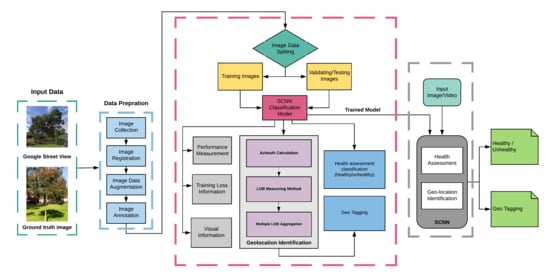
3. Material and Methods
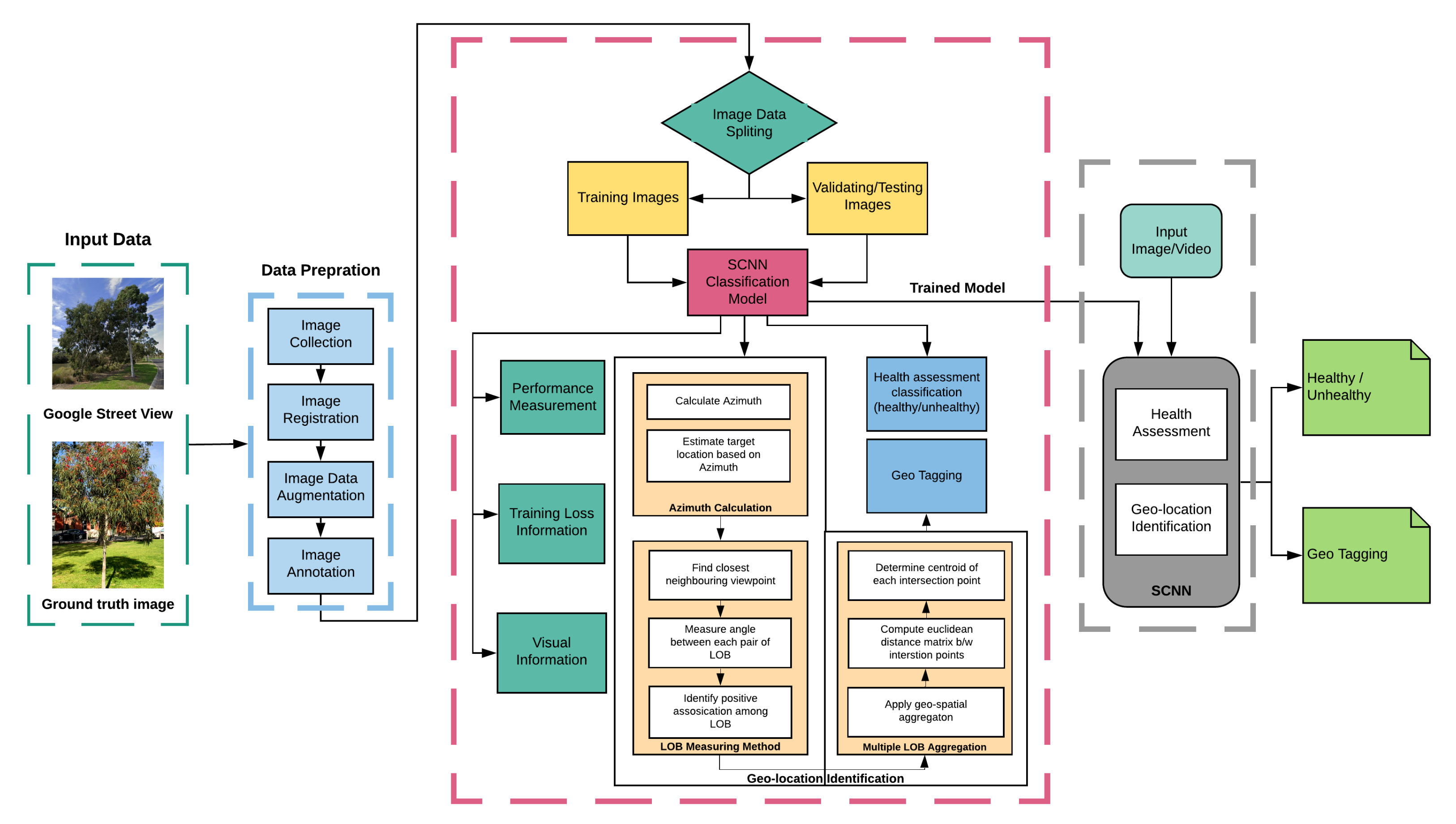
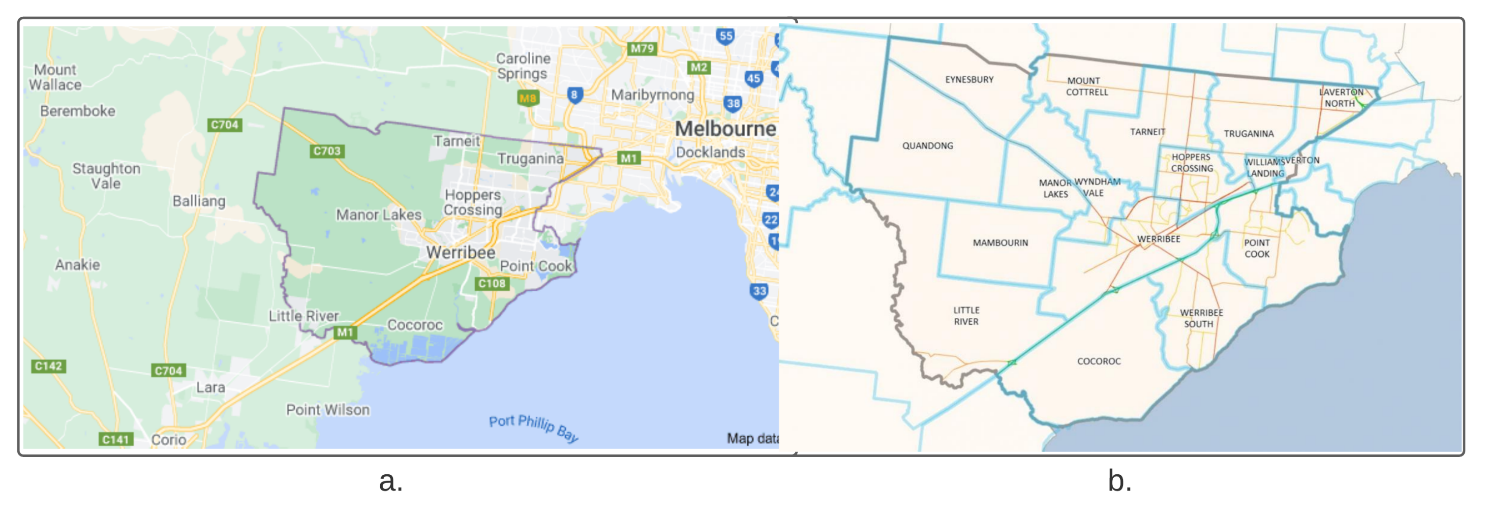
3.1. Study Area and GIS Data
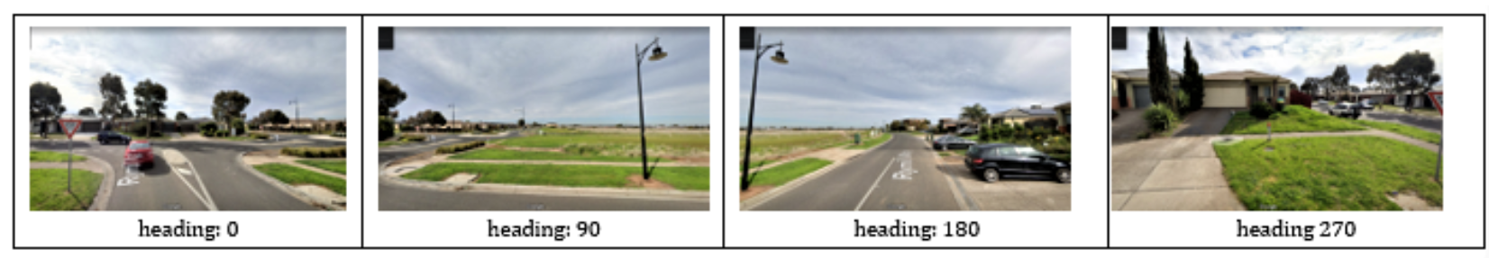
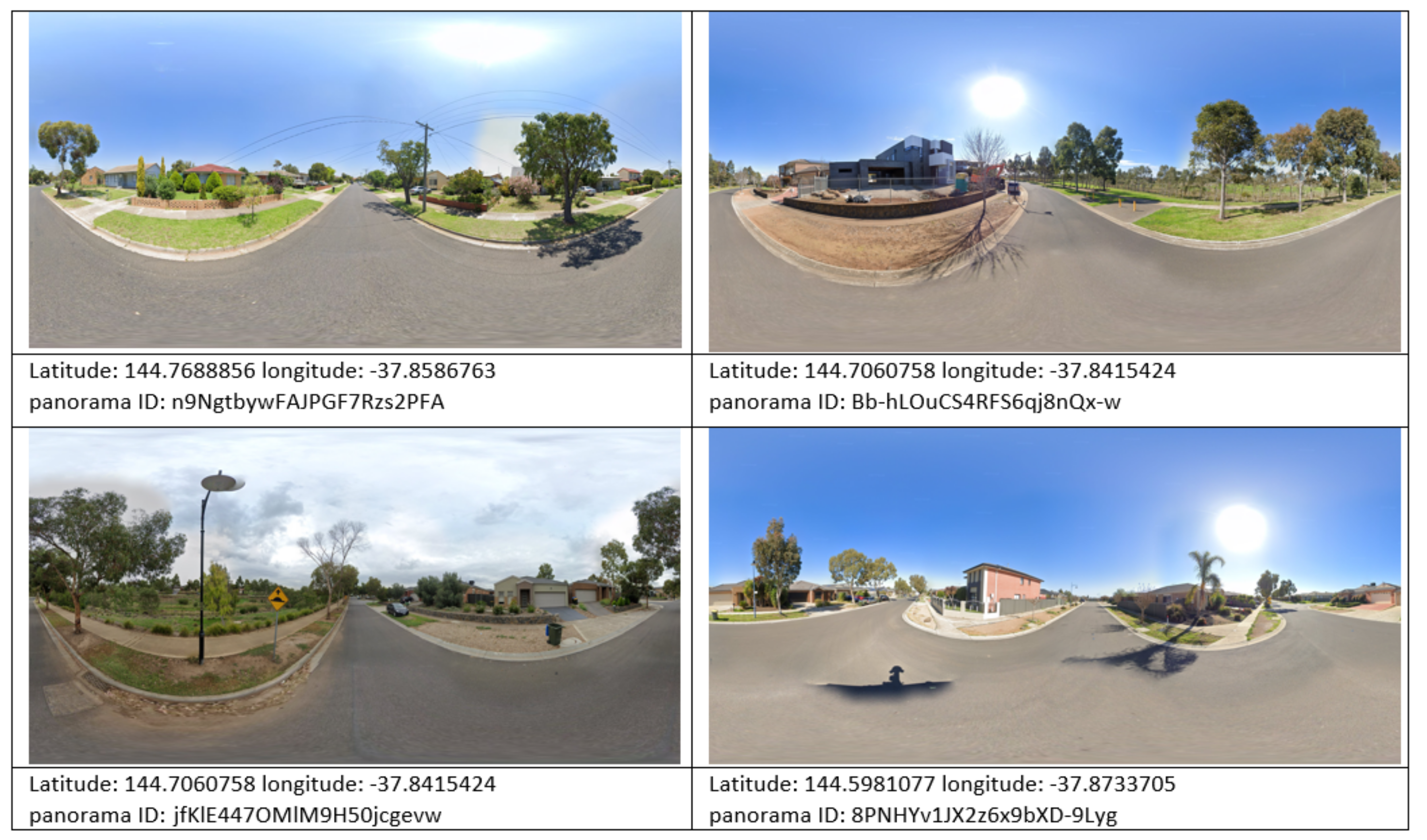
3.2. Google Street View (GSV) Imagery
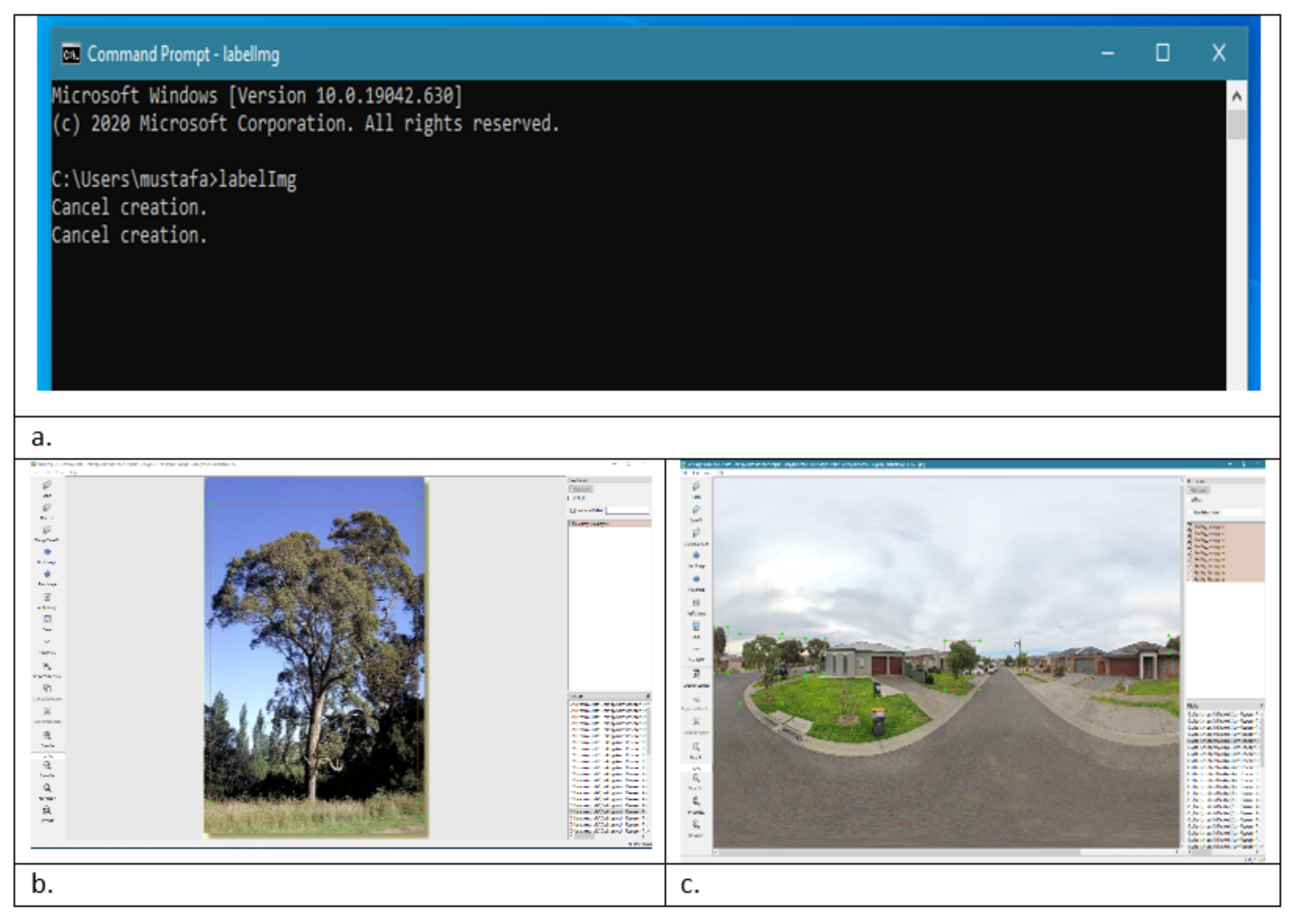
3.3. Annotation Data
3.4. Training Siamese CNN
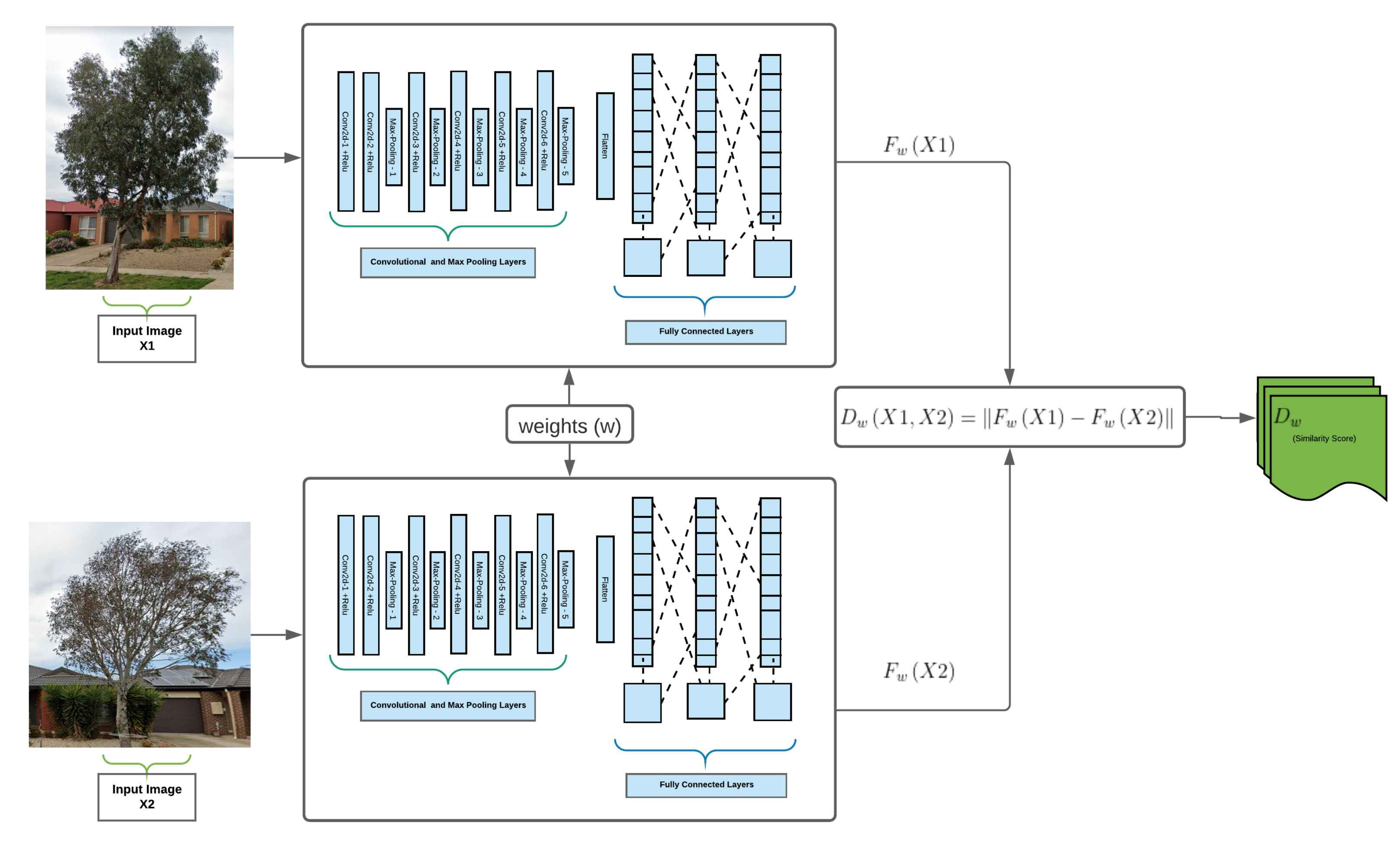
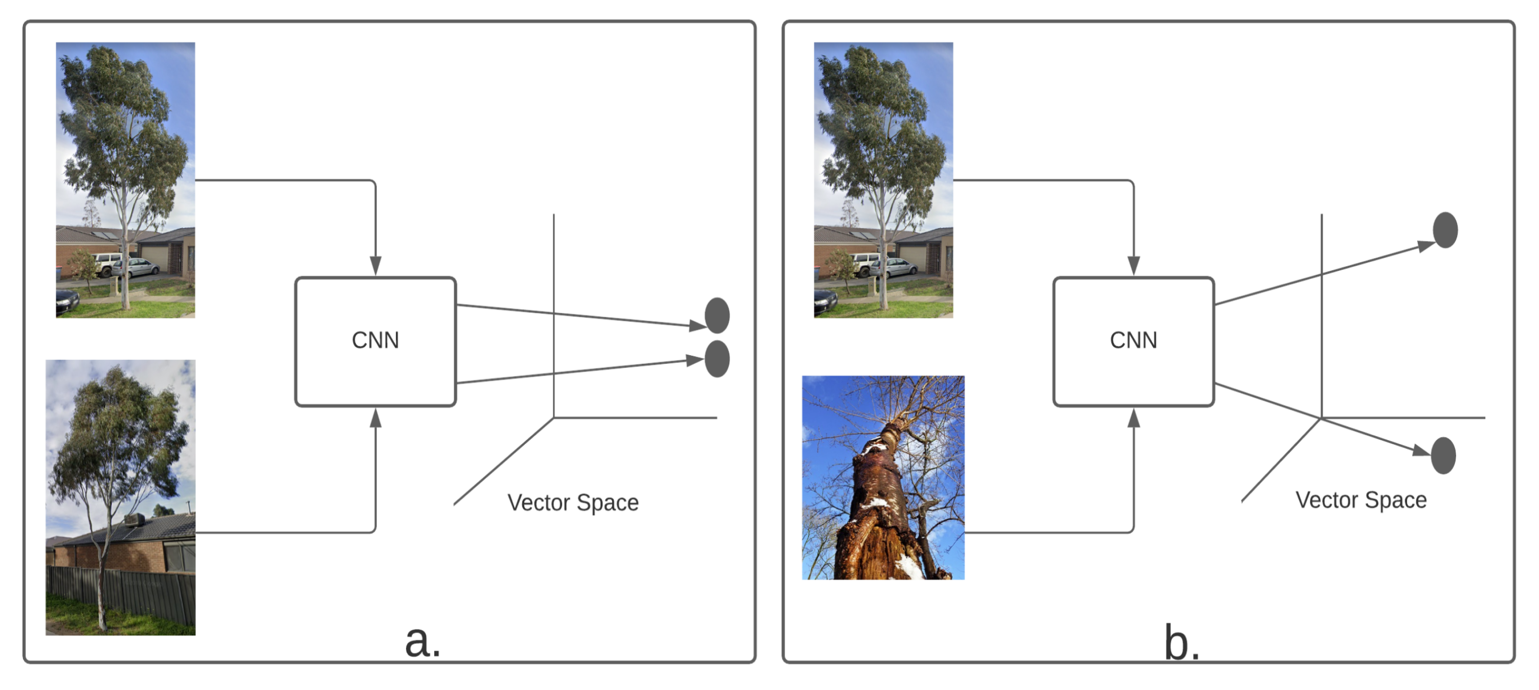
3.5. Siamese CNN Architecture
3.5.1. Contrastive Loss Function
3.5.2. Mapping to Binary Function
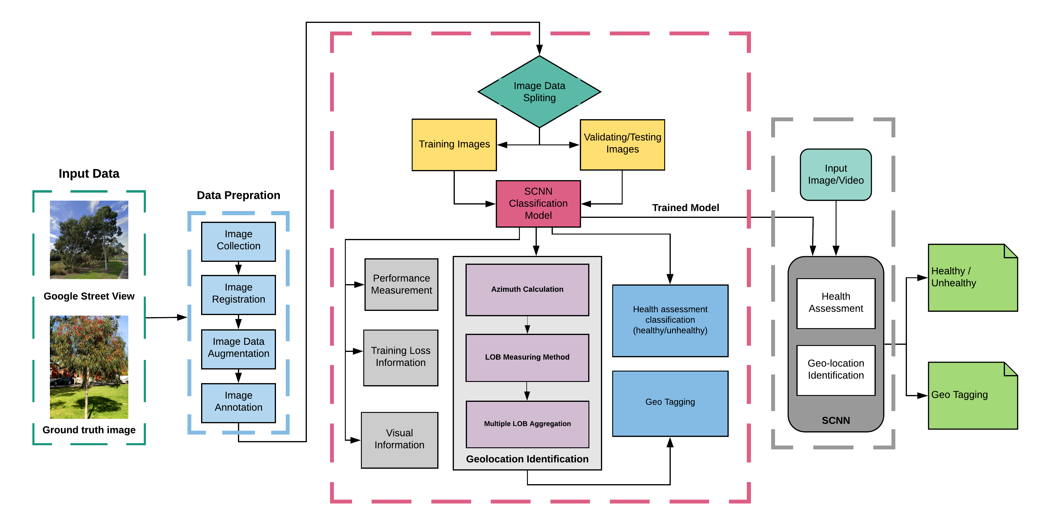
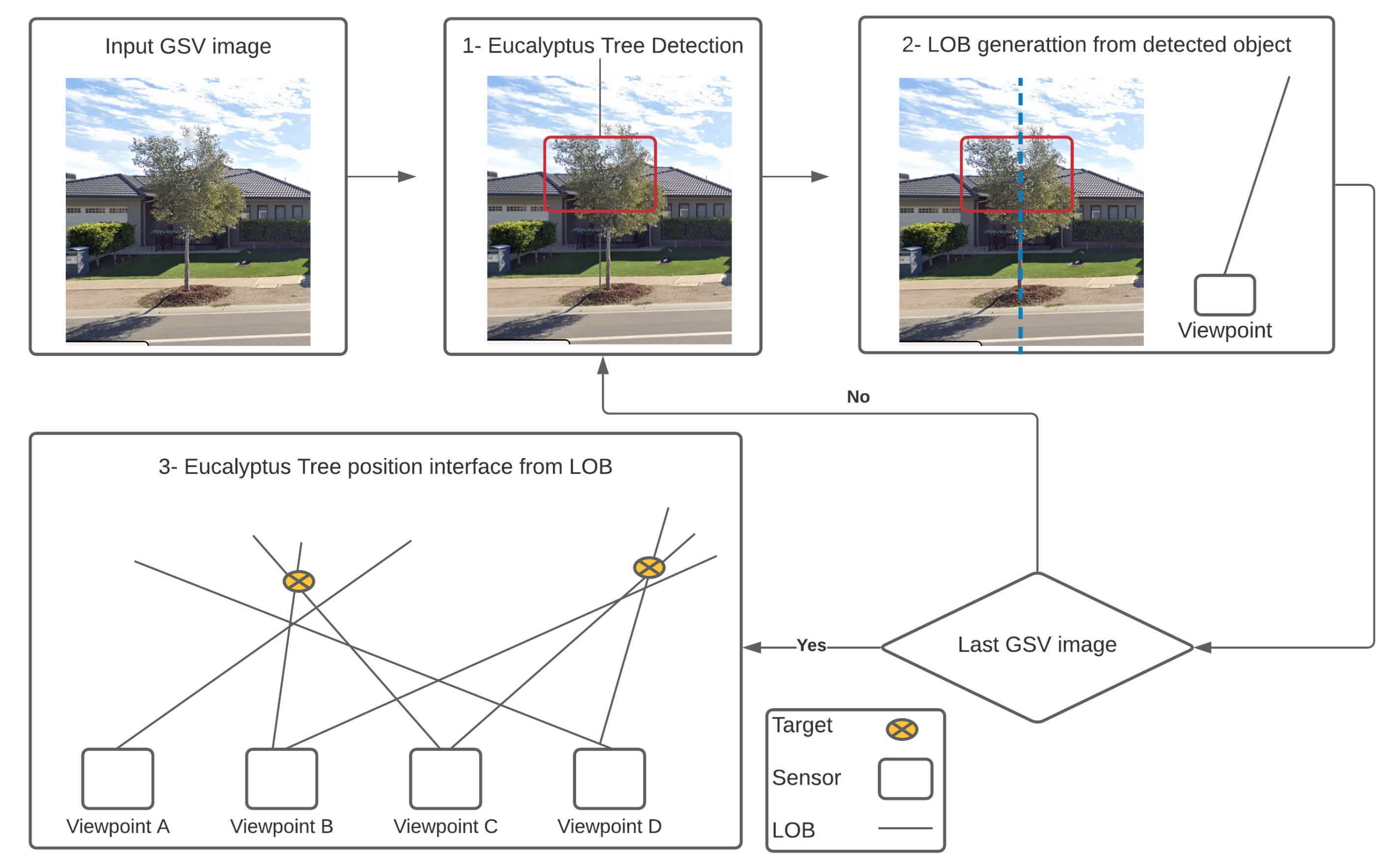
3.6. Geolocation Identification
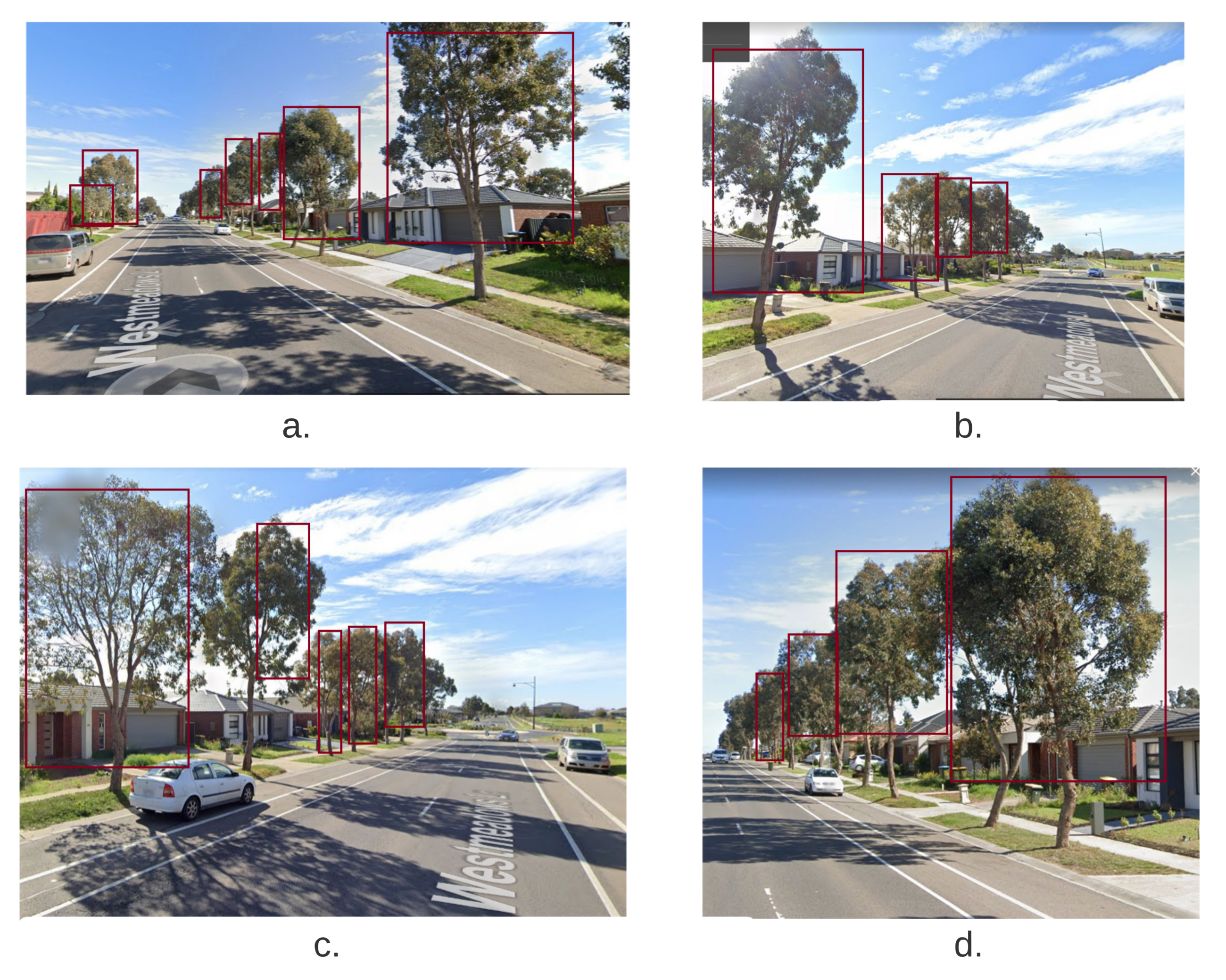
- Detect Eucalyptus tree in the GSV images using a trained DL network.
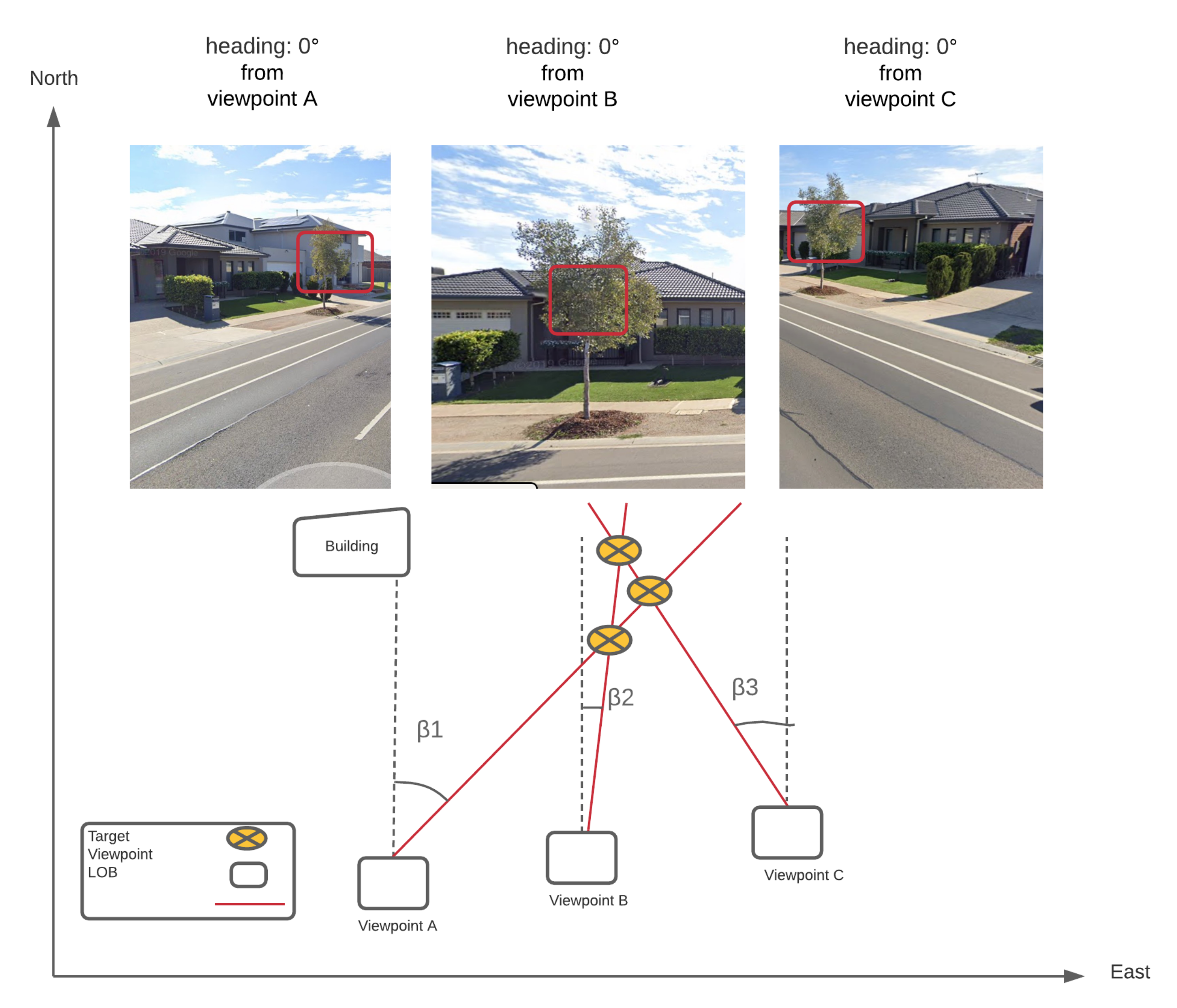
- Calculate the azimuth from each viewpoint to the detected Eucalyptus tree based on the known azimuth angles of the GSV images, relative to their view point locations, and the horizontal positions of the target in the images as shown in Figure 8 (2) using the mean value of two X values of the bounding box. For instance; suppose a detected Eucalyptus tree has a bounding box that is centered on column 228 in a GSV image that is centered at 0° azimuth relative to the image viewpoint. Each GSV image contains 640 columns and spans a 90° horizontal field-of-view; thus, each pixel spans 0.14. The center of the Eucalyptus tree is 130 pixels to the right of the image center (at column 320) and so has an azimuth of 18.2° relative to the image viewpoint. “Azimuth is an angle formed by a reference vector in a reference plane pointing towards (but not necessarily meeting) something of interest and a second vector in the same plane. For instance, With the sea as your reference plane, the Sun’s azimuth may be defined as the angle between due North and the point on the horizon where the Sun is currently visible. A hypothetical line drawn parallel to the sea’s surface could point in the Sun’s direction but never meet it.” [72].
- The final step is to estimate the target locations based on the azimuths calculated from the second step as presented in Figure 8 (3).
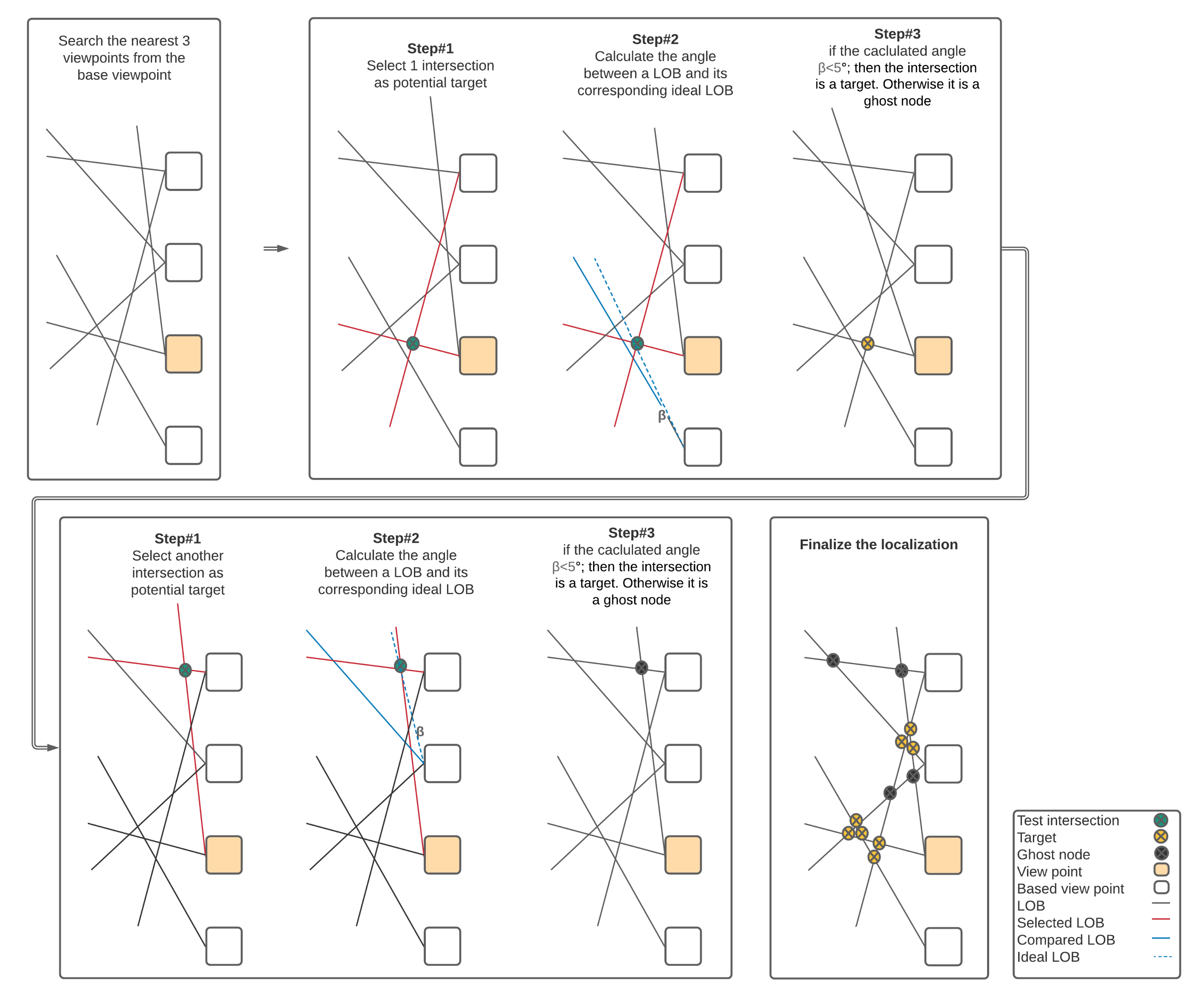
3.6.1. LOB Measurement Method
- Targets and sensors are in the xy plane, and
- All LOB measurements are of equal precision [77].
- Find the closest neighboring viewpoints for a given viewpoint; we tested the algorithm’s performance using 2 to 8 of the closest neighboring viewpoints (i.e., the corresponding number of views is 3 to 9).
- Measure the angles between each pair of LOBs from all viewpoints [78].
- Check whether there are positive associations among LOBs (set at 50 m length) from current viewpoint and its neighboring viewpoints.
- Repeat the process from step 1 to step 3 for every intersection point.
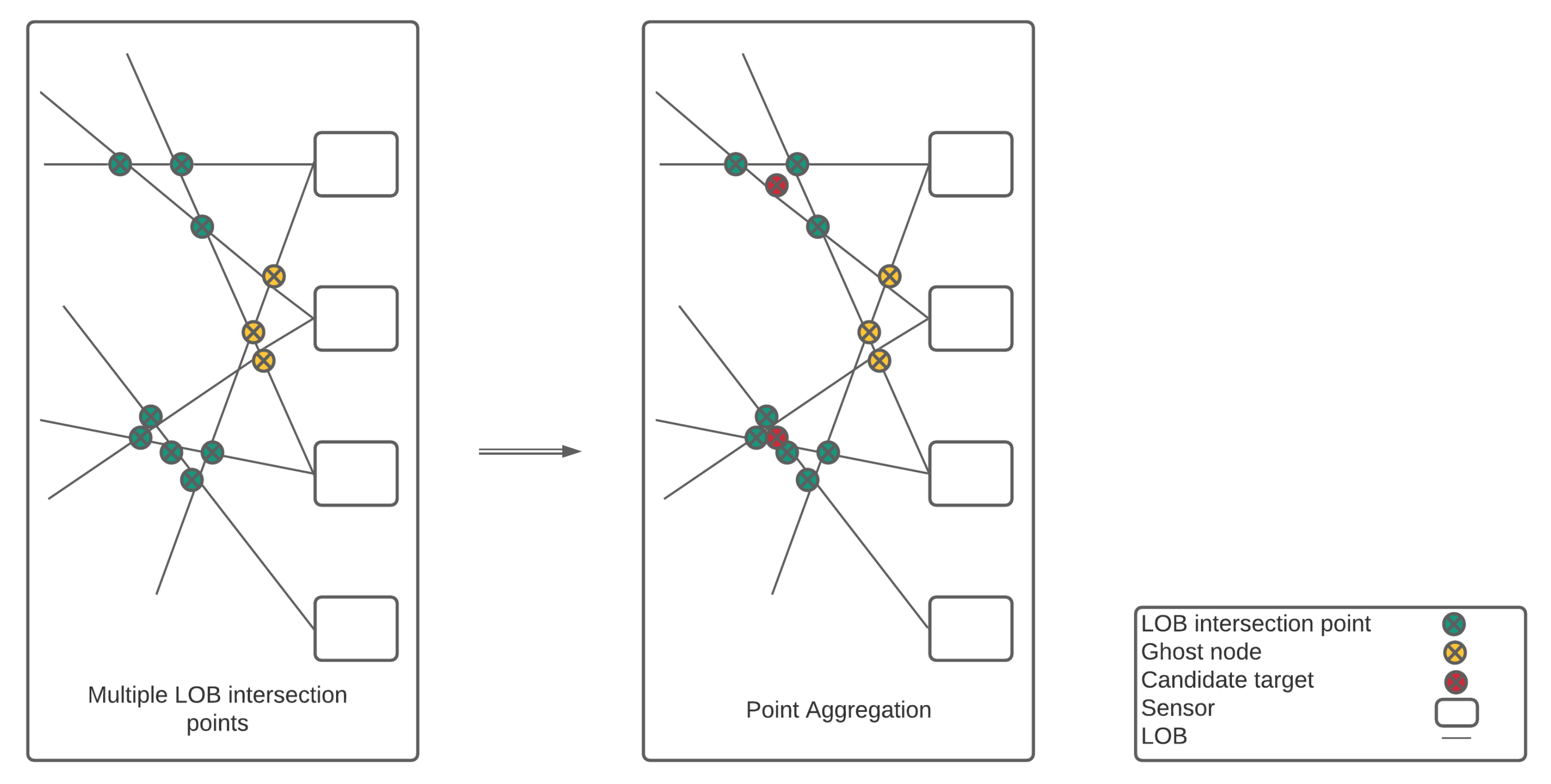
3.6.2. Multiple LOB Intersection Points Aggregation
- Compute the Euclidean distance matrix between all LOB intersection points.
- The Euclidean distances between LOB intersection points are used to cluster LOB intersection points.
- Determine the centroid of each intersection point cluster.
3.6.3. Spatial Aggregation and Calculation of Points
4. Experiments and Results
4.1. Experiments
4.2. System Configuration
4.3. Approach
4.4. Results
Location Estimation Accuracy Evaluation
5. Discussion
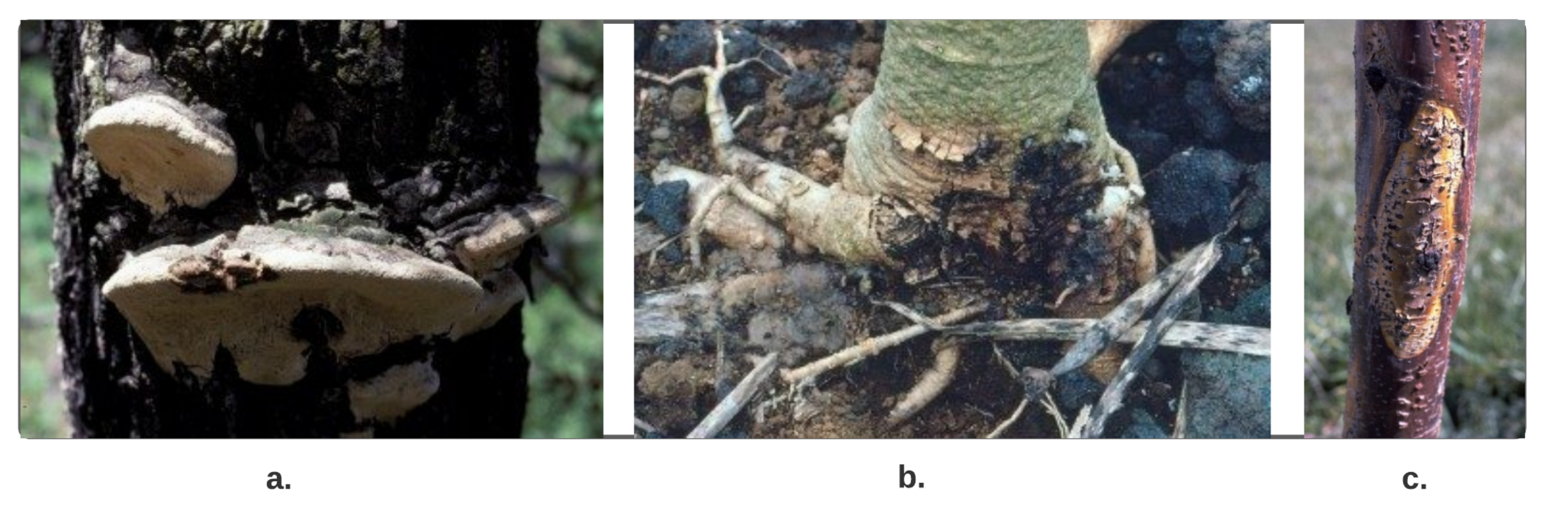
- a.
- Canker disease that infects the bark and then goes inside of the tree,
- b.
- Phytophthora disease goes directly under the bark by discolored leaves and dark brown wood, and
- c.
- The heart disease damages the tree from inside and outside.
6. Conclusions, Limitations, and Future Directions
Author Contributions
Funding
Institutional Review Board Statement
Informed Consent Statement
Data Availability Statement
Conflicts of Interest
References
- Branson, S.; Wegner, J.D.; Hall, D.; Lang, N.; Schindler, K.; Perona, P. From Google Maps to a fine-grained catalog of street trees. ISPRS J. Photogramm. Remote Sens. 2018, 135, 13–30. [Google Scholar] [CrossRef]
- Salmond, J.A.; Tadaki, M.; Vardoulakis, S.; Arbuthnott, K.; Coutts, A.; Demuzere, M.; Dirks, K.N.; Heaviside, C.; Lim, S.; Macintyre, H.; et al. Health and climate related ecosystem services provided by street trees in the urban environment. Environ. Health 2016, 15, 95–111. [Google Scholar] [CrossRef] [PubMed]
- Ladiges, P. The Story of Our Eucalypts—Curious. Available online: https://www.science.org.au/curious/earth-environment/story-our-eucalypts (accessed on 4 January 2021).
- Eucalypt Forest—Department of Agriculture. Available online: https://www.agriculture.gov.au/abares/forestsaustralia/profiles/eucalypt-2016 (accessed on 4 January 2021).
- Berrang, P.; Karnosky, D.F.; Stanton, B.J. Environmental factors affecting tree health in New York City. J. Arboric. 1985, 11, 185–189. [Google Scholar]
- Cregg, B.M.; Dix, M.E. Tree moisture stress and insect damage in urban areas in relation to heat island effects. J. Arboric. 2001, 27, 8–17. [Google Scholar]
- Winn, M.F.; Lee, S.M.; Araman, P.A. Urban tree crown health assessment system: A tool for communities and citizen foresters. In Proceedings of the Proceedings, Emerging Issues Along Urban-Rural Interfaces II: Linking Land-Use Science and Society, Atlanta, GA, USA, 9–12 April 2007; pp. 180–183. [Google Scholar]
- Czerniawska-Kusza, I.; Kusza, G.; Dużyński, M. Effect of deicing salts on urban soils and health status of roadside trees in the Opole region. Environ. Toxicol. Int. J. 2004, 19, 296–301. [Google Scholar] [CrossRef]
- Day, S.D.; Bassuk, N.L. A review of the effects of soil compaction and amelioration treatments on landscape trees. J. Arboric. 1994, 20, 9–17. [Google Scholar]
- Doody, T.; Overton, I. Environmental management of riparian tree health in the Murray-Darling Basin, Australia. River Basin Manag. V 2009, 124, 197. [Google Scholar]
- Butt, N.; Pollock, L.J.; McAlpine, C.A. Eucalypts face increasing climate stress. Ecol. Evol. 2013, 3, 5011–5022. [Google Scholar] [CrossRef]
- Chicco, D. Siamese neural networks: An overview. Artificial Neural Networks; Springer: New York, NY, USA, 2021; pp. 73–94. [Google Scholar]
- About Us—Wyndham City. Available online: https://www.wyndham.vic.gov.au/about-us (accessed on 4 January 2021).
- Google Street View Imagery—Google Search. Available online: https://www.google.com/search?q=google+street+view+imagery&rlz=1C1CHBF_en-GBAU926AU926&oq=google+&aqs=chrome.1.69i57j35i39l2j69i60l2j69i65j69i60l2.7725j0j4&sourceid=chrome&ie=UTF-8 (accessed on 4 January 2021).
- Anguelov, D.; Dulong, C.; Filip, D.; Frueh, C.; Lafon, S.; Lyon, R.; Ogale, A.; Vincent, L.; Weaver, J. Google street view: Capturing the world at street level. Computer 2010, 43, 32–38. [Google Scholar] [CrossRef]
- Li, X.; Zhang, C.; Li, W.; Ricard, R.; Meng, Q.; Zhang, W. Assessing street-level urban greenery using Google Street View and a modified green view index. Urban For. Urban Green. 2015, 14, 675–685. [Google Scholar] [CrossRef]
- Li, X.; Zhang, C.; Li, W.; Kuzovkina, Y.A.; Weiner, D. Who lives in greener neighborhoods? The distribution of street greenery and its association with residents’ socioeconomic conditions in Hartford, Connecticut, USA. Urban For. Urban Green. 2015, 14, 751–759. [Google Scholar] [CrossRef]
- Li, X.; Zhang, C.; Li, W. Building block level urban land-use information retrieval based on Google Street View images. GIScience Remote Sens. 2017, 54, 819. [Google Scholar] [CrossRef]
- Zhang, W.; Li, W.; Zhang, C.; Hanink, D.M.; Li, X.; Wang, W. Parcel-based urban land use classification in megacity using airborne LiDAR, high resolution orthoimagery, and Google Street View. Comput. Environ. Urban Syst. 2017, 64, 215–228. [Google Scholar] [CrossRef]
- Li, X.; Ratti, C.; Seiferling, I. Quantifying the shade provision of street trees in urban landscape: A case study in Boston, USA, using Google Street View. Landsc. Urban Plan. 2018, 169, 81–91. [Google Scholar] [CrossRef]
- Khan, A.; Nawaz, U.; Ulhaq, A.; Robinson, R.W. Real-time plant health assessment via implementing cloud-based scalable transfer learning on AWS DeepLens. PLoS ONE 2020, 15. [Google Scholar] [CrossRef]
- Khan, A.; Ulhaq, A.; Robinson, R.; Ur Rehman, M. Detection of Vegetation in Environmental Repeat Photography: A New Algorithmic Approach in Data Science; Statistics for Data Science and Policy Analysis; Rahman, A., Ed.; Springer: Singapore, 2020; pp. 145–157. [Google Scholar]
- Tumas, P.; Nowosielski, A.; Serackis, A. Pedestrian detection in severe weather conditions. IEEE Access 2020, 8, 62775–62784. [Google Scholar] [CrossRef]
- Guo, G.; Wang, H.; Yan, Y.; Zheng, J.; Li, B. A fast face detection method via convolutional neural network. Neurocomputing 2020, 395, 128–137. [Google Scholar] [CrossRef]
- Wu, J.; Song, L.; Wang, T.; Zhang, Q.; Yuan, J. Forest r-cnn: Large-vocabulary long-tailed object detection and instance segmentation. In Proceedings of the 28th ACM International Conference on Multimedia, Seattle, WA, USA, 12–16 October 2020; pp. 1570–1578. [Google Scholar]
- Islam, M.M.; Yang, H.C.; Poly, T.N.; Jian, W.S.; Li, Y.C.J. Deep learning algorithms for detection of diabetic retinopathy in retinal fundus photographs: A systematic review and meta-analysis. Comput. Methods Programs Biomed. 2020, 191, 105320. [Google Scholar] [CrossRef]
- Zeng, D.; Yu, F. Research on the Application of Big Data Automatic Search and Data Mining Based on Remote Sensing Technology. In Proceedings of the 2020 3rd International Conference on Artificial Intelligence and Big Data (ICAIBD), Chengdu, China, 28–31 May 2020; pp. 122–127. [Google Scholar]
- Voulodimos, A.; Doulamis, N.; Doulamis, A.; Protopapadakis, E. Deep learning for computer vision: A brief review. Comput. Intell. Neurosci. 2018, 2018, 7068349. [Google Scholar] [CrossRef]
- Miltiadou, M.; Campbell, N.D.; Aracil, S.G.; Brown, T.; Grant, M.G. Detection of dead standing Eucalyptus camaldulensis without tree delineation for managing biodiversity in native Australian forest. Int. J. Appl. Earth Obs. Geoinf. 2018, 67, 135–147. [Google Scholar] [CrossRef]
- Shendryk, I.; Broich, M.; Tulbure, M.G.; Alexandrov, S.V. Bottom-up delineation of individual trees from full-waveform airborne laser scans in a structurally complex eucalypt forest. Remote Sens. Environ. 2016, 173, 69–83. [Google Scholar] [CrossRef]
- Kamińska, A.; Lisiewicz, M.; Stereńczak, K.; Kraszewski, B.; Sadkowski, R. Species-related single dead tree detection using multi-temporal ALS data and CIR imagery. Remote Sens. Environ. 2018, 219, 31–43. [Google Scholar] [CrossRef]
- Weinmann, M.; Weinmann, M.; Mallet, C.; Brédif, M. A classification-segmentation framework for the detection of individual trees in dense MMS point cloud data acquired in urban areas. Remote Sens. 2017, 9, 277. [Google Scholar] [CrossRef]
- Briechle, S.; Krzystek, P.; Vosselman, G. Classification of tree species and standing dead trees by fusing UAV-based lidar data and multispectral imagery in the 3D deep neural network PointNet++. ISPRS Ann. Photogramm. Remote Sens. Spat. Inf. Sci. 2020, 5, 203–210. [Google Scholar] [CrossRef]
- Mollaei, Y.; Karamshahi, A.; Erfanifard, S. Detection of the Dry Trees Result of Oak Borer Beetle Attack Using Worldview-2 Satellite and UAV Imagery an Object-Oriented Approach. J Remote Sens. GIS 2018, 7, 2. [Google Scholar] [CrossRef]
- Yao, W.; Krzystek, P.; Heurich, M. Identifying standing dead trees in forest areas based on 3D single tree detection from full waveform lidar data. ISPRS Ann. Protogrammetry, Remote Sens. Spat. Inf. Sci. 2012, 1, 7. [Google Scholar] [CrossRef]
- Deng, X.; Lan, Y.; Hong, T.; Chen, J. Citrus greening detection using visible spectrum imaging and C-SVC. Comput. Electron. Agric. 2016, 130, 177–183. [Google Scholar] [CrossRef]
- Lan, Y.; Huang, Z.; Deng, X.; Zhu, Z.; Huang, H.; Zheng, Z.; Lian, B.; Zeng, G.; Tong, Z. Comparison of machine learning methods for citrus greening detection on UAV multispectral images. Comput. Electron. Agric. 2020, 171, 105234. [Google Scholar] [CrossRef]
- Shendryk, I.; Broich, M.; Tulbure, M.G.; McGrath, A.; Keith, D.; Alexandrov, S.V. Mapping individual tree health using full-waveform airborne laser scans and imaging spectroscopy: A case study for a floodplain eucalypt forest. Remote Sens. Environ. 2016, 187, 202–217. [Google Scholar] [CrossRef]
- Meng, R.; Dennison, P.E.; Zhao, F.; Shendryk, I.; Rickert, A.; Hanavan, R.P.; Cook, B.D.; Serbin, S.P. Mapping canopy defoliation by herbivorous insects at the individual tree level using bi-temporal airborne imaging spectroscopy and LiDAR measurements. Remote Sens. Environ. 2018, 215, 170–183. [Google Scholar] [CrossRef]
- López-López, M.; Calderón, R.; González-Dugo, V.; Zarco-Tejada, P.J.; Fereres, E. Early detection and quantification of almond red leaf blotch using high-resolution hyperspectral and thermal imagery. Remote Sens. 2016, 8, 276. [Google Scholar] [CrossRef]
- Barnes, C.; Balzter, H.; Barrett, K.; Eddy, J.; Milner, S.; Suárez, J.C. Airborne laser scanning and tree crown fragmentation metrics for the assessment of Phytophthora ramorum infected larch forest stands. For. Ecol. Manag. 2017, 404, 294–305. [Google Scholar] [CrossRef]
- Fassnacht, F.E.; Latifi, H.; Ghosh, A.; Joshi, P.K.; Koch, B. Assessing the potential of hyperspectral imagery to map bark beetle-induced tree mortality. Remote Sens. Environ. 2014, 140, 533–548. [Google Scholar] [CrossRef]
- Chi, D.; Degerickx, J.; Yu, K.; Somers, B. Urban Tree Health Classification Across Tree Species by Combining Airborne Laser Scanning and Imaging Spectroscopy. Remote Sens. 2020, 12, 2435. [Google Scholar] [CrossRef]
- Näsi, R.; Honkavaara, E.; Lyytikäinen-Saarenmaa, P.; Blomqvist, M.; Litkey, P.; Hakala, T.; Viljanen, N.; Kantola, T.; Tanhuanpää, T.; Holopainen, M. Using UAV-based photogrammetry and hyperspectral imaging for mapping bark beetle damage at tree-level. Remote Sens. 2015, 7, 15467–15493. [Google Scholar] [CrossRef]
- Näsi, R.; Honkavaara, E.; Blomqvist, M.; Lyytikäinen-Saarenmaa, P.; Hakala, T.; Viljanen, N.; Kantola, T.; Holopainen, M. Remote sensing of bark beetle damage in urban forests at individual tree level using a novel hyperspectral camera from UAV and aircraft. Urban For. Urban Green. 2018, 30, 72–83. [Google Scholar] [CrossRef]
- Degerickx, J.; Roberts, D.A.; McFadden, J.P.; Hermy, M.; Somers, B. Urban tree health assessment using airborne hyperspectral and LiDAR imagery. Int. J. Appl. Earth Obs. Geoinf. 2018, 73, 26–38. [Google Scholar] [CrossRef]
- Xiao, Q.; McPherson, E.G. Tree health mapping with multispectral remote sensing data at UC Davis, California. Urban Ecosyst. 2005, 8, 349–361. [Google Scholar] [CrossRef]
- Goldbergs, G.; Maier, S.W.; Levick, S.R.; Edwards, A. Efficiency of individual tree detection approaches based on light-weight and low-cost UAS imagery in Australian Savannas. Remote Sens. 2018, 10, 161. [Google Scholar] [CrossRef]
- Fassnacht, F.E.; Mangold, D.; Schäfer, J.; Immitzer, M.; Kattenborn, T.; Koch, B.; Latifi, H. Estimating stand density, biomass and tree species from very high resolution stereo-imagery – towards an all-in-one sensor for forestry applications? For. Int. J. For. Res. 2017, 90, 613–631. [Google Scholar] [CrossRef]
- Li, W.; He, C.; Fu, H.; Zheng, J.; Dong, R.; Xia, M.; Yu, L.; Luk, W. A Real-Time Tree Crown Detection Approach for Large-Scale Remote Sensing Images on FPGAs. Remote Sens. 2019, 11, 1025. [Google Scholar] [CrossRef]
- Ruiz, V.; Linares, I.; Sanchez, A.; Velez, J.F. Off-line handwritten signature verification using compositional synthetic generation of signatures and Siamese Neural Networks. Neurocomputing 2020, 374, 30–41. [Google Scholar] [CrossRef]
- Zhao, X.; Zhou, S.; Lei, L.; Deng, Z. Siamese network for object tracking in aerial video. In Proceedings of the 2018 IEEE 3rd International Conference on Image, Vision and Computing (ICIVC), Chongqing, China, 27–29 June 2018; pp. 519–523. [Google Scholar]
- Rao, D.J.; Mittal, S.; Ritika, S. Siamese Neural Networks for One-Shot Detection of Railway Track Switches. Available online: https://arxiv.org/abs/1712.08036 (accessed on 21 December 2017).
- Chandra, M.; Redkar, S.; Roy, S.; Patil, P. Classification of Various Plant Diseases Using Deep Siamese Network. Available online: https://www.researchgate.net/profile/Manish-Chandra-3/publication/341322315_CLASSIFICATION_OF_VARIOUS_PLANT_DISEASES_USING_DEEP_SIAMESE_NETWORK/links/5ebaa82f299bf1c09ab52e48/CLASSIFICATION-OF-VARIOUS-PLANT-DISEASES-USING-DEEP-SIAMESE-NETWORK.pdf (accessed on 12 May 2020).
- Shorfuzzaman, M.; Hossain, M.S. MetaCOVID: A Siamese neural network framework with contrastive loss for n-shot diagnosis of COVID-19 patients. Pattern Recognit. 2020, 113, 107700. [Google Scholar] [CrossRef]
- Bromley, J.; Bentz, J.W.; Bottou, L.; Guyon, I.; Lecun, Y.; Moore, C.; Säckinger, E.; Shah, R. Signature Verification Using a “Siamese” Time Delay Neural Network. Int. J. Pattern Recognit. Artif. Intell. 1993, 07, 669–688. [Google Scholar] [CrossRef]
- Wang, B.; Wang, D. Plant Leaves Classification: A Few-Shot Learning Method Based on Siamese Network. IEEE Access 2019, 7, 27008–27016. [Google Scholar] [CrossRef]
- Wyndham City Suburbs | Wyndham City Advocacy. Available online: https://wyndham-digital.iconagency.com.au/node/10 (accessed on 4 January 2021).
- What Is an Application Programming Interface (API)? | IBM. Available online: https://www.ibm.com/cloud/learn/api (accessed on 4 January 2021).
- Berners-Lee, T.; Masinter, L.; McCahill, M. Uniform Resource Locators. 1994. Available online: https://dl.acm.org/doi/book/10.17487/RFC1738 (accessed on 28 May 2021).
- GitHub-Robolyst/Streetview: Python Module for Retrieving Current and Historical Photos from Google Street View. Available online: https://github.com/robolyst/streetview (accessed on 1 April 2021).
- GitHub-Tzutalin/labelImg: LabelImg Is a Graphical Image Annotation Tool and Label Object Bounding Boxes in Images. Available online: https://github.com/tzutalin/labelImg (accessed on 1 April 2021).
- A Friendly Introduction to Siamese Networks | by Sean Benhur J | Towards Data Science. Available online: https://towardsdatascience.com/a-friendly-introduction-to-siamese-networks-85ab17522942 (accessed on 1 April 2021).
- Zhang, K.; Zuo, W.; Gu, S.; Zhang, L. Learning deep CNN denoiser prior for image restoration. In Proceedings of the IEEE Conference on Computer Vision and Pattern Recognition, Honolulu, HI, USA, 21–26 July 2017; pp. 3929–3938. [Google Scholar]
- Santurkar, S.; Tsipras, D.; Ilyas, A.; Madry, A. How does batch normalization help optimization? In Proceedings of the Advances in Neural Information Processing Systems, Montréal, QC, Canada, 2–8 December 2018; pp. 2483–2493. [Google Scholar]
- Li, Y.; Yuan, Y. Convergence analysis of two-layer neural networks with relu activation. In Proceedings of the Advances in Neural Information Processing Systems, Long Beach, CA, 4–9 December 2017; pp. 597–607. [Google Scholar]
- Dunne, R.A.; Campbell, N.A. On the Pairing of the Softmax Activation and Cross-Entropy Penalty Functions and the Derivation of the Softmax Activation Function. Available online: https://citeseerx.ist.psu.edu/viewdoc/download?doi=10.1.1.49.6403&rep=rep1&type=pdf (accessed on 28 May 2021).
- Nassar, A.S.; Lefèvre, S.; Wegner, J.D. Multi-View Instance Matching with Learned Geometric Soft-Constraints. ISPRS Int. J. Geo-Inf. 2020, 9, 687. [Google Scholar] [CrossRef]
- Contrastive Loss Explained. Contrastive Loss Has Been Used Recently… | by Brian Williams | Towards Data Science. Available online: https://towardsdatascience.com/contrastive-loss-explaned-159f2d4a87ec (accessed on 4 January 2021).
- Chopra, S.; Hadsell, R.; LeCun, Y. Learning a similarity metric discriminatively, with application to face verification. In Proceedings of the 2005 IEEE Computer Society Conference on Computer Vision and Pattern Recognition (CVPR’05), San Diego, CA, USA, 20–25 June 2005; Volume 1, pp. 539–546. [Google Scholar]
- Hadsell, R.; Chopra, S.; LeCun, Y. Dimensionality reduction by learning an invariant mapping. In Proceedings of the 2006 IEEE Computer Society Conference on Computer Vision and Pattern Recognition (CVPR’06), New York, NY, USA, 17–22 June 2006; Volume 2, pp. 1735–1742. [Google Scholar]
- Rutstrum, C. The Wilderness Route Finder; Collier Books: New York, NY, USA; Collier-Macmillan Publishers: London, UK, 1967. [Google Scholar]
- Gavish, M.; Weiss, A. Performance analysis of bearing-only target location algorithms. IEEE Trans. Aerosp. Electron. Syst. 1992, 28, 817–828. [Google Scholar] [CrossRef]
- Zhang, H.; Jing, Z.; Hu, S. Localization of Multiple Emitters Based on the Sequential PHD Filter. Signal Process. 2010, 90, 34–43. [Google Scholar] [CrossRef]
- Reed, J.D.; da Silva, C.R.; Buehrer, R.M. Multiple-source localization using line-of-bearing measurements: Approaches to the data association problem. In Proceedings of the MILCOM 2008-2008 IEEE Military Communications Conference, San Diego, CA, USA, 16–19 November 2008; pp. 1–7. [Google Scholar]
- Grabbe, M.T.; Hamschin, B.M.; Douglas, A.P. A measurement correlation algorithm for line-of-bearing geo-location. In Proceedings of the 2013 IEEE Aerospace Conference, Big Sky, MT, USA, 3–10 March 2013; pp. 1–8. [Google Scholar]
- Tan, K.; Chen, H.; Cai, X. Research into the algorithm of false points elimination in three-station cross location. Shipboard Electron. Countermeas 2009, 32, 79–81. [Google Scholar]
- Reed, J. Approaches to Multiple Source Localization and Signal Classification. Ph.D. Thesis, Virginia Tech, Blacksburg, VA, USA, 2009. [Google Scholar]
- Spatial Aggregation—ArcGIS Insights | Documentation. Available online: https://doc.arcgis.com/en/insights/latest/analyze/spatial-aggregation.htm (accessed on 1 May 2021).
- Rao, A.S.; What Do You Mean by GIS Aggregation. Geography Knowledge Hub. 2016. Available online: https://www.publishyourarticles.net/knowledge-hub/geography/what-do-you-mean-by-gis-aggregation/1298/ (accessed on 28 May 2021).
- Ketkar, N. Introduction to keras. In Deep Learning with Python; Springer: New York, NY, USA, 2017; pp. 97–111. [Google Scholar]
- Ketkar, N. Introduction to Tensorflow. In Deep Learning with Python; Springer: New York, NY, USA, 2017; pp. 159–194. [Google Scholar]
- Alippi, C.; Disabato, S.; Roveri, M. Moving convolutional neural networks to embedded systems: The alexnet and VGG-16 case. In Proceedings of the 2018 17th ACM/IEEE International Conference on Information Processing in Sensor Networks (IPSN), Porto, Portugal, 11–13 April 2018; pp. 212–223. [Google Scholar]
- Tran, D.; Wang, H.; Torresani, L.; Ray, J.; LeCun, Y.; Paluri, M. A closer look at spatiotemporal convolutions for action recognition. In Proceedings of the IEEE Conference on Computer Vision and Pattern Recognition, Salt Lake City, UT, USA, 18–23 June 2018; pp. 6450–6459. [Google Scholar]
- Szegedy, C.; Ioffe, S.; Vanhoucke, V.; Alemi, A. Inception-v4, inception-resnet and the impact of residual connections on learning. arXiv 2016, arXiv:1602.07261. [Google Scholar]
- Pedregosa, F.; Varoquaux, G.; Gramfort, A.; Michel, V.; Thirion, B.; Grisel, O.; Blondel, M.; Prettenhofer, P.; Weiss, R.; Dubourg, V.; et al. Scikit-learn: Machine Learning in Python. J. Mach. Learn. Res. 2011, 12, 2825–2830. [Google Scholar]
- Weight Initialization in Neural Networks: A Journey From the Basics to Kaiming | by James Dellinger | Towards Data Science. Available online: https://towardsdatascience.com/weight-initialization-in-neural-networks-a-journey-from-the-basics-to-kaiming-954fb9b47c79 (accessed on 4 January 2021).
- 4 Signs That Your Tree Is Dying | Perth Arbor Services. Available online: https://pertharborservices.com.au/4-signs-your-tree-is-dying-what-to-do/ (accessed on 4 January 2021).
- Common Eucalyptus Tree Problems: Eucalyptus Tree Diseases. Available online: https://www.gardeningknowhow.com/ornamental/trees/eucalyptus/eucalyptus-tree-problems.htm (accessed on 4 January 2021).
- How Often Does Google Maps Update Satellite Images? | Techwalla. Available online: https://www.techwalla.com/articles/how-often-does-google-maps-update-satellite-images (accessed on 15 May 2021).
- 9 Things to Know about Google’s Maps Data: Beyond the Map | Google Cloud Blog. Available online: https://cloud.google.com/blog/products/maps-platform/9-things-know-about-googles-maps-data-beyond-map (accessed on 15 May 2021).


| Evaluation Metrics | Value in % |
|---|---|
| Precision | 93.38% |
| Recall | 92.98% |
| Accuracy | 93.2% |
| F1-Score | 92.17% |
| Number of Views | Threshold of Angle (°) | Threshold of Distance to Center of Selected Road (m) | Percentage of the Number of Estimated Locations of Eucalyptus Tree Being within a Certain Buffer Zone of Reference Eucalyptus Tree (%) | Number of Estimated Eucalyptus Tree | |||||||||
|---|---|---|---|---|---|---|---|---|---|---|---|---|---|
| <1 m | <2 m | <3 m | <4 m | <5 m | <6 m | <7 m | <8 m | <9 m | <10 m | ||||
| 1 | 3 | 1.75 | 8.04 | 22.38 | 35.66 | 46.85 | 54.9 | 62.59 | 68.18 | 74.83 | 80.07 | 286 | |
| 1 | 4 | 1.83 | 8.42 | 23.44 | 36.63 | 47.62 | 55.68 | 64.47 | 70.7 | 76.92 | 82.42 | 273 | |
| 1 | 5 | 1.92 | 7.69 | 23.08 | 37.31 | 49.23 | 57.69 | 67.31 | 72.69 | 79.23 | 85 | 260 | |
| 2 | 3 | 1.71 | 8.05 | 19.51 | 30.98 | 44.88 | 53.41 | 58.78 | 64.63 | 72.93 | 77.8 | 410 | |
| 3 | 2 | 4 | 1.75 | 8.27 | 19.8 | 31.08 | 45.36 | 53.88 | 60.15 | 66.92 | 74.94 | 79.95 | 399 |
| 2 | 5 | 1.85 | 8.71 | 20.32 | 32.72 | 47.76 | 56.73 | 63.59 | 69.66 | 77.31 | 82.32 | 379 | |
| 3 | 3 | 2.37 | 8.84 | 20.47 | 31.9 | 43.32 | 50.86 | 57.54 | 64.01 | 71.12 | 75.86 | 464 | |
| 3 | 4 | 2.68 | 8.95 | 20.36 | 31.77 | 43.18 | 51.23 | 58.17 | 65.55 | 72.93 | 77.18 | 447 | |
| 3 | 5 | 2.56 | 9.3 | 20 | 32.79 | 44.88 | 53.02 | 60.23 | 66.98 | 74.65 | 79.53 | 430 | |
| 1 | 3 | 2 | 7.56 | 19.56 | 30.89 | 40.67 | 51.33 | 58 | 63.11 | 71.11 | 76 | 450 | |
| 1 | 4 | 1.87 | 7.26 | 20.37 | 30.91 | 42.62 | 53.86 | 60.89 | 67.45 | 74.71 | 79.16 | 427 | |
| 1 | 5 | 2.02 | 7.83 | 20.96 | 32.32 | 44.44 | 55.81 | 63.38 | 70.45 | 77.78 | 83.33 | 396 | |
| 2 | 3 | 1.31 | 7.86 | 17.84 | 29.13 | 39.44 | 48.12 | 54.99 | 62.52 | 67.76 | 72.83 | 611 | |
| 4 | 2 | 4 | 1.2 | 7.72 | 18.01 | 29.5 | 41.68 | 51.29 | 58.32 | 65.87 | 71.7 | 76.33 | 583 |
| 2 | 5 | 1.09 | 8.56 | 18.58 | 30.78 | 43.53 | 53.37 | 60.47 | 68.12 | 74.32 | 79.05 | 549 | |
| 3 | 3 | 1.35 | 7.77 | 16.89 | 29 | 38.42 | 46.79 | 55.31 | 62.78 | 68.76 | 74.14 | 669 | |
| 3 | 4 | 1.39 | 8.19 | 18.08 | 30.45 | 40.96 | 49.15 | 57.5 | 65.84 | 71.56 | 76.82 | 647 | |
| 3 | 5 | 1.47 | 9.61 | 19.06 | 30.94 | 42.51 | 50.98 | 59.45 | 68.4 | 74.43 | 78.99 | 614 | |
| 1 | 3 | 2.2 | 10.8 | 22.34 | 35.35 | 45.6 | 51.83 | 57.51 | 64.29 | 71.98 | 77.47 | 546 | |
| 1 | 4 | 2.46 | 11 | 22.35 | 36.36 | 48.48 | 55.3 | 61.93 | 68.94 | 75.19 | 79.17 | 528 | |
| 1 | 5 | 2.63 | 11.3 | 22.63 | 37.37 | 49.7 | 56.97 | 63.84 | 71.92 | 77.78 | 83.23 | 495 | |
| 2 | 3 | 2.31 | 11 | 19.62 | 30.3 | 42.14 | 48.77 | 57.58 | 64.36 | 71.28 | 75.47 | 693 | |
| 5 | 2 | 4 | 2.53 | 10.3 | 19.2 | 32.44 | 45.83 | 53.27 | 61.61 | 68.3 | 73.66 | 77.98 | 672 |
| 2 | 5 | 2.52 | 10.2 | 19.69 | 32.6 | 47.72 | 55.28 | 63.15 | 70.08 | 77.17 | 81.57 | 635 | |
| 3 | 3 | 2.37 | 10.4 | 19.05 | 29.17 | 39.55 | 47.83 | 56.37 | 63.34 | 69.51 | 74.24 | 761 | |
| 3 | 4 | 2.84 | 10.4 | 19.08 | 30.72 | 42.63 | 51.42 | 60.35 | 66.98 | 72.26 | 76.73 | 739 | |
| 3 | 5 | 3.01 | 11.1 | 20.23 | 32.28 | 43.9 | 53.52 | 62.41 | 70.01 | 76.33 | 80.63 | 697 | |
| 1 | 3 | 2.5 | 12.2 | 23.21 | 36.06 | 46.41 | 52.92 | 60.27 | 67.78 | 73.12 | 78.46 | 599 | |
| 1 | 4 | 2.87 | 12.2 | 23.99 | 37.67 | 48.14 | 54.56 | 63.18 | 70.78 | 74.32 | 78.55 | 592 | |
| 1 | 5 | 2.5 | 12.9 | 25.04 | 38.64 | 49.91 | 57.07 | 65.47 | 73.7 | 78 | 82.47 | 559 | |
| 2 | 3 | 2.43 | 10.8 | 21.62 | 33.92 | 44.73 | 52.3 | 59.86 | 65.14 | 71.76 | 78.24 | 740 | |
| 6 | 2 | 4 | 2.46 | 10.3 | 21.61 | 34.75 | 47.74 | 56.5 | 64.71 | 70.86 | 74.69 | 79.07 | 731 |
| 2 | 5 | 2.47 | 11.2 | 23.11 | 36.63 | 50.44 | 59.88 | 67.3 | 73.4 | 78.05 | 82.27 | 688 | |
| 3 | 3 | 2.22 | 9.75 | 20.49 | 32.47 | 41.23 | 50.49 | 57.9 | 63.21 | 70.62 | 75.43 | 810 | |
| 3 | 4 | 2.63 | 10.1 | 21.13 | 33.88 | 44.5 | 55.38 | 62.88 | 68.63 | 73.25 | 76.63 | 800 | |
| 3 | 5 | 2.76 | 10.8 | 22.97 | 34.78 | 46.19 | 57.09 | 64.44 | 70.47 | 76.12 | 79.4 | 762 | |
| 1 | 3 | 2.7 | 12.4 | 24.01 | 38.31 | 49.92 | 56.6 | 63.28 | 68.68 | 74.72 | 79.81 | 629 | |
| 1 | 4 | 2.91 | 12.4 | 25.36 | 41.03 | 52.67 | 58.16 | 65.59 | 72.54 | 77.71 | 82.23 | 619 | |
| 1 | 5 | 2.74 | 13.2 | 27.05 | 43.15 | 55.65 | 60.96 | 69.01 | 75.34 | 80.65 | 84.93 | 584 | |
| 2 | 3 | 2.2 | 9.95 | 21.71 | 34.24 | 44.44 | 52.07 | 59.56 | 65.37 | 70.8 | 76.36 | 774 | |
| 7 | 2 | 4 | 2.61 | 9.52 | 23.21 | 36.64 | 47.72 | 56.19 | 64.15 | 70.01 | 73.14 | 77.84 | 767 |
| 2 | 5 | 2.37 | 10.6 | 23.29 | 38.35 | 51.05 | 59.14 | 67.78 | 73.08 | 77.82 | 82.01 | 717 | |
| 3 | 3 | 2.75 | 10.2 | 22.04 | 33.53 | 43.95 | 52.22 | 59.28 | 66.35 | 72.1 | 75.57 | 835 | |
| 3 | 4 | 3.15 | 10.2 | 23.12 | 35.23 | 46.25 | 55.33 | 62.47 | 68.77 | 72.88 | 76.15 | 826 | |
| 3 | 5 | 3.31 | 11.5 | 23.92 | 36.01 | 48.6 | 56.87 | 65.14 | 70.99 | 75.95 | 79.64 | 786 | |
| 1 | 3 | 3.08 | 12.2 | 25.08 | 40.92 | 52.92 | 58.77 | 64.77 | 70.46 | 70.46 | 76.77 | 650 | |
| 1 | 4 | 3.87 | 12.9 | 26.63 | 43.03 | 55.42 | 60.84 | 66.41 | 73.68 | 78.17 | 82.51 | 646 | |
| 1 | 5 | 4.08 | 13.7 | 28.22 | 45.02 | 58.4 | 63.62 | 70.47 | 77.16 | 82.54 | 86.79 | 613 | |
| 2 | 3 | 3.44 | 11.3 | 23.66 | 36.01 | 47.2 | 54.33 | 61.58 | 65.52 | 70.74 | 75.7 | 786 | |
| 8 | 2 | 4 | 3.68 | 11.3 | 25.51 | 37.44 | 50 | 57.61 | 64.47 | 69.16 | 72.21 | 76.78 | 788 |
| 2 | 5 | 3.49 | 12.1 | 26.71 | 39.19 | 52.62 | 59.46 | 67.65 | 72.89 | 77.18 | 80.54 | 745 | |
| 3 | 3 | 3.05 | 11.2 | 23.12 | 34.62 | 45.42 | 52.93 | 60.09 | 66.2 | 71.24 | 75.7 | 852 | |
| 3 | 4 | 3.51 | 11.2 | 24.09 | 35.79 | 47.6 | 56.02 | 61.99 | 69.36 | 72.4 | 76.02 | 855 | |
| 3 | 5 | 3.78 | 13.3 | 25.61 | 38.66 | 49.88 | 57.44 | 65.73 | 71.71 | 76.1 | 79.63 | 820 | |
| 1 | 3 | 2.67 | 11.7 | 24.67 | 41.46 | 52.15 | 58.99 | 65.53 | 71.92 | 76.37 | 82.91 | 673 | |
| 1 | 4 | 2.85 | 12 | 26.39 | 42.73 | 54.72 | 61.62 | 66.87 | 73.01 | 77.21 | 82.01 | 667 | |
| 1 | 5 | 3.14 | 13.8 | 28.57 | 45.84 | 58.87 | 64.52 | 70.8 | 76.77 | 81.16 | 85.71 | 637 | |
| 2 | 3 | 3.18 | 11.3 | 22.03 | 36.72 | 47.37 | 54.59 | 61.57 | 65.97 | 70.26 | 75.64 | 817 | |
| 9 | 2 | 4 | 3.04 | 12.2 | 23.45 | 37.3 | 48.97 | 57.23 | 62.33 | 67.8 | 71.08 | 75.7 | 823 |
| 2 | 5 | 3.47 | 12.5 | 25.06 | 40.36 | 51.8 | 59.13 | 66.07 | 71.47 | 75.45 | 78.92 | 778 | |
| 3 | 3 | 2.95 | 11.4 | 22.05 | 36.36 | 47.16 | 54.77 | 60.91 | 65.8 | 70.11 | 75.34 | 880 | |
| 3 | 4 | 2.83 | 12.2 | 23.42 | 36.88 | 49.21 | 56.56 | 62.44 | 67.99 | 71.15 | 75.23 | 884 | |
| 3 | 5 | 3.4 | 12.9 | 24.74 | 39.98 | 51.11 | 58.15 | 64.95 | 71.04 | 75.38 | 78.55 | 853 | |
Publisher’s Note: MDPI stays neutral with regard to jurisdictional claims in published maps and institutional affiliations. |
© 2021 by the authors. Licensee MDPI, Basel, Switzerland. This article is an open access article distributed under the terms and conditions of the Creative Commons Attribution (CC BY) license (https://creativecommons.org/licenses/by/4.0/).
Share and Cite
Khan, A.; Asim, W.; Ulhaq, A.; Ghazi, B.; Robinson, R.W. Health Assessment of Eucalyptus Trees Using Siamese Network from Google Street and Ground Truth Images. Remote Sens. 2021, 13, 2194. https://doi.org/10.3390/rs13112194
Khan A, Asim W, Ulhaq A, Ghazi B, Robinson RW. Health Assessment of Eucalyptus Trees Using Siamese Network from Google Street and Ground Truth Images. Remote Sensing. 2021; 13(11):2194. https://doi.org/10.3390/rs13112194
Chicago/Turabian StyleKhan, Asim, Warda Asim, Anwaar Ulhaq, Bilal Ghazi, and Randall W. Robinson. 2021. "Health Assessment of Eucalyptus Trees Using Siamese Network from Google Street and Ground Truth Images" Remote Sensing 13, no. 11: 2194. https://doi.org/10.3390/rs13112194
APA StyleKhan, A., Asim, W., Ulhaq, A., Ghazi, B., & Robinson, R. W. (2021). Health Assessment of Eucalyptus Trees Using Siamese Network from Google Street and Ground Truth Images. Remote Sensing, 13(11), 2194. https://doi.org/10.3390/rs13112194