Abstract
Urban greenery is an essential characteristic of the urban ecosystem, which offers various advantages, such as improved air quality, human health facilities, storm-water run-off control, carbon reduction, and an increase in property values. Therefore, identification and continuous monitoring of the vegetation (trees) is of vital importance for our urban lifestyle. This paper proposes a deep learning-based network, Siamese convolutional neural network (SCNN), combined with a modified brute-force-based line-of-bearing (LOB) algorithm that evaluates the health of Eucalyptus trees as healthy or unhealthy and identifies their geolocation in real time from Google Street View (GSV) and ground truth images. Our dataset represents Eucalyptus trees’ various details from multiple viewpoints, scales and different shapes to texture. The experiments were carried out in the Wyndham city council area in the state of Victoria, Australia. Our approach obtained an average accuracy of 93.2% in identifying healthy and unhealthy trees after training on around 4500 images and testing on 500 images. This study helps in identifying the Eucalyptus tree with health issues or dead trees in an automated way that can facilitate urban green management and assist the local council to make decisions about plantation and improvements in looking after trees. Overall, this study shows that even in a complex background, most healthy and unhealthy Eucalyptus trees can be detected by our deep learning algorithm in real time.
1. Introduction
Street trees are an essential feature of urban or metropolitan areas, although relatively ignored. Their benefits include air filtering, water interception, cooling, minimising energy consumption, erosion reduction, pollution management, and run-off detection [1,2]. Various trees are planted in urban areas due to street trees’ social, economic and environmental advantages. One such tree, Eucalyptus, is a valuable asset for communities in urban areas of Australia. Eucalyptus trees are icons of the Australian flora, often called gum trees. They dominate the Australian landscape with more than 800 species, forming forests, woodlands and shrub-lands in all environments, except for the aridest deserts. Evidence from DNA sequencing and fossil discovery shows that Eucalyptus had its evolutionary roots in Gondwana when Australia was still linked to Antarctica [3]. Traditionally, indigenous Australians have used almost all parts of Eucalyptus trees. Leaves and leaf oils have medicinal properties, and saps may be used as adhesive resins; bark and wood were used to make vessels, tools and weapons, such as spears and clubs [4]. For the conservation of Australia’s rich biodiversity, Eucalyptus native forests are significant.
There are two factors that are detrimental to the health of street trees. First, urban trees are under persistent strain, i.e., excessive soil moisture and soil mounding in nurseries on roots that have an adverse effect on their health [5]. Secondly, urban ecosystem distinguished by elevated peak temperatures relative to nearby rural areas [6], soil compaction, limited growth of roots, pollution of groundwater [7], and high air pollution concentrations caused by community activities. Usually, urban soil contains a significant volume of static building waste, contaminants, de-icing salts, low soil quality and a significant degree of volume density, thus maintaining a low natural activity and the inferior organic material substance provided [8,9]. Both of these reasons raise the likelihood of water and nutrient pressure, which degrades the metabolism and development of a tree and reduces its capacity to provide ecosystem services. Urban tree conditions are adversely affected due to soil compaction, low hydraulic conductivity, low compaction aeration and mostly insufficient available rooting space [9]. In addition, inadequate conditions at the site raise the threat of insect disease and infestation [6].
The evaluation of tree health conditions is highly critical for biodiversity, forest management, global environmental monitoring and carbon dynamics. Unhealthy tree features are identifiable and can build a detection and classification model using deep learning to intelligently diagnose Eucalyptus in a healthy and unsanitary/dead tree. To consider the importance of urban trees to the community, they should be adequately maintained, including obstacle prevention, regeneration, and substitution of dead or unhealthy trees. Ideally, skilled green managers need to monitor the precise and consistent spatial data on tree’s health. About 60% of the riparian tree vegetation in extensive wetlands and floodplains reported being in poor health, or extinct [10]. Chronic decreases are associated with extreme weather conditions due to human resources management, various pathogens, pests and various parasites. Trees are stressed [11] in the landscape, where the soil has a poor drainage mechanism, also resulting in low growth of trees. The most common factors such as soil erosion, nutrient deficiency, allelopathy, biodiversity, pests, and diseases affect Eucalyptus species’ health.
Detection and recognition of Eucalyptus tree health presents a challenging task since many trees have a few pixels across input images, and some trees are also overshadowed by other trees and cannot be found due to weather conditions or lighting. For addressing these challenges and achieving high accuracy and precise prediction, a large amount of labelled training data for feature extraction of healthy and unhealthy class features is required. For this purpose, we used GSV imagery and ground truth images were obtained from various viewpoints and at different times. This study uses the Siamese Convolutional Neural Network (SCNN) [12], to develop an automated model for identification and classification and a line-of-bearing measurement approach paired with a spatial aggregation approach is used to estimate the geolocation of the Eucalyptus tree. We concentrated on the identification of healthy and unhealthy Eucalyptus trees along the streets and roads in the Wyndham city council area [13]. This study aims to use a self-created ground truth and GSV [14] imagery for finding the geolocation, identification and classification of healthy and unhealthy Eucalyptus trees to prevent damage that can significantly reduce ecosystem harm and financial loss. GSV is an open image series of streetwise panoramic views with approximate precise geolocation details acquired on mobile platforms using GPS, wheel encoder, and inertial navigation sensor (using multiple sources such as cars, trekkers and boats) [15]. This GSV has been widely used to increase geographical information in a variety of areas of interest, including urban greenery [16,17], land use classification [18,19] and tree shade provision [20].
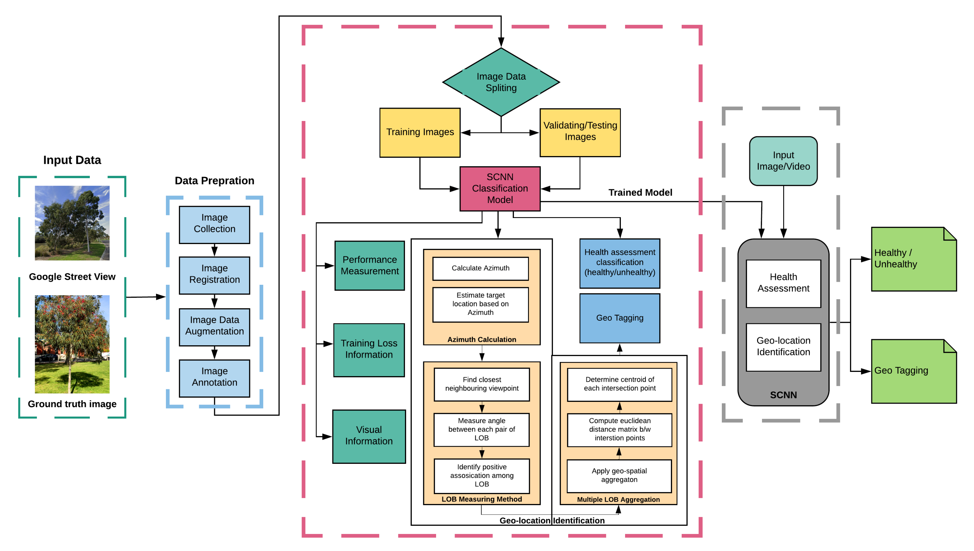
Our key contributions are (a.) classification of trees that are in a healthy or unhealthy state and (b.) identification of geolocation of the Eucalyptus trees. All these evaluations are done based on GSV imagery and self-gathered ground truth image data from streets. Our experiments show that this proposed method can effectively detect and classify healthy and unhealthy Eucalyptus trees with various dataset and complex backgrounds. Our proposed method for geolocation identification gives us reliable results and could be applied for geo-identification of other objects on the roadside. Figure 1 shows the overall visual representation of this study.
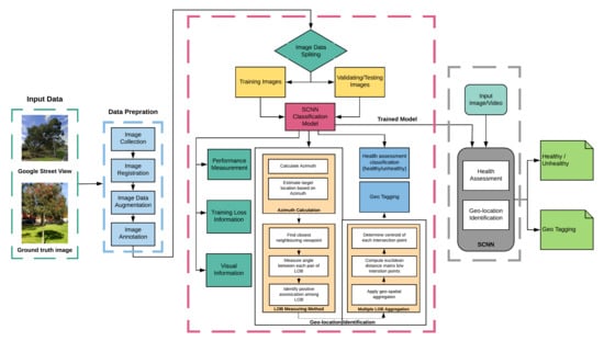
Figure 1.
General workflow diagram of classifying healthy or unhealthy and geo-tagging Eucalyptus trees from GSV and ground truth images.
2. Related Work
Numerous work has been done on detection and recognition in various areas such as fruits and vegetable plant leaves disease detection [21], vegetation detection [22], pedestrian detection [23], face detection [24], object detection [25], using various deep learning algorithms [26]. Automatic data analysis in the remote sensing (RS) [27] and computer vision [28] field is of vital significance. RS data have been used in urban areas to assess trees health. A large volume of the study shows various RS techniques used to determine the current condition of trees. In contrast, on the other side, a minimal amount of research shows interest in the identification and classification of dead trees. Milto Miltiadou et al. [29] presented a new way to detect dead Eucalyptus camaldulensis with the introduction of DASOS (feature vector extraction). They tried to explore the probability of dead trees detection without tree demidruleation from Voxel-based full-waveform (FW) LiDAR. Shendryk et al. [30] suggested a bottom-up algorithm to detect Eucalyptus tree trunks and the demidruleation of individual trees with complex shapes. Agnieszka Kamińska et al. [31] used remote sensing techniques, including airborne laser scanner and colour infrared imagery, to classify between living or dead trees and concluded that only airborne laser scanner detects dead tree at the single tree level.
Martin Weinmann et al. [32] proposed a novel two-step approach to detect a single tree in heavily sampled 3D point cloud data obtained from urban locations and tackled semantical classification by assignment of semantic class labelling to irregularly separated 3D points and semantic segmentation by separating individual items within the named 3D points. S. Briechle et al. [33] worked on the PointNet++ 3D deep neural network with the combination of imagery data (LiDAR and multispectral) to classify various species as well as standing dead tree crowns. The values of laser echo pulse width and multispectral characteristics were also introduced into the classification process, and individual tree’s 3D segments were created in a pre-processing stage of a 3D detection system. Yousef Taghi Mollaei et al. [34] developed an object-oriented model using high-resolution images to map the pest-dried trees. The findings confirm that the object-oriented approach can classify the dried surfaces with precise detail and high accuracy. W. Yao et al. [35] proposed an approach to individual dead tree identification using LiDAR data in mountain forests. The three-dimensional coordinates were derived from laser beam reflexes, pulse intensity and width using waveform breakdowns and 3D single trees were then detected by an optimized method that describes both the dominated trees and small under-story trees within the canopy model.
According to Xiaoling Deng et al. [36,37] machine learning has been used to set several benchmarks in the field of agriculture. W. Yao et al. [35] and Shendryk et al. [38] published their prior work on the identification of dead trees is performed by individual tree crown segmentation prior to the health assessment. Meng R. et al. [39], Shendryk et al. [30], López-López M et al. [40], Barnes et al. [41], Fassnacht et al. [42], mentioned that most of the current tree health studies centred either on evaluating the defoliation of the tree crown or the overall health status of the tree, although there was minimal exposure to the discolouration of the tree crown. Dengkai et al. [43] used a group of fields assessed tree health indicators to define tree health that was classified with a Random Forest classifier using airborne laser scanning (ALS) data and hyperspectral imagery (HSI). They compared the outcomes of ALS data and HIS and also their combination and then analysed the accuracy degree of classification. Nasi et al. [44,45] reported in two different pieces of research that the potential of UAV-based photogrammetry and HSI for mapping bark beetle in an urban forest, damage at tree level. Degerickx et al. [46] performed tree health classification based on chlorophyll and leaf area index derived from HSI, where for individual tree crown segmentation, they used ALS data. Xiao et al. [47] used normalised difference vegetation index (NDVI) to detect healthy and unhealthy trees. They found it challenging to map tree health across various species or in places where many tree species coexist. Goldbergs et al. [48] evaluated local maxima and watershed models for the detection of individual trees, and they found the efficient performance of these models for dominant and co-dominant trees. Fabian et al. [49] presented their work on random forest regression to predict total trees using local maxima and a classification process to identify a tree, soil and shadow. Li et al. [50] introduced a Field-Programmable Gate Array (FPGA) for tree crown detection, significantly rapid calculations without loss of functioning.
Siamese network [12] has been used in a variety of applications, including signature verification [51], object tracking [52], railway track switches [53], plant leaves disease detection [54], and coronavirus diseases detection [55]. Bromley et al. [56] proposed a neural network model for signature matching by introducing for the very first time Siamese network. Bin Wang et al. [57] presented a few-shot learning method for leaf classification with a small sample size based on the Siamese network. However, we are using a Siamese convolutional neural network (SCNN) combined with a modified brute-force-based line-of-bearing (LOB) algorithm to classify Eucalyptus trees as healthy or unhealthy and to find their geolocation.
3. Material and Methods
3.1. Study Area and GIS Data
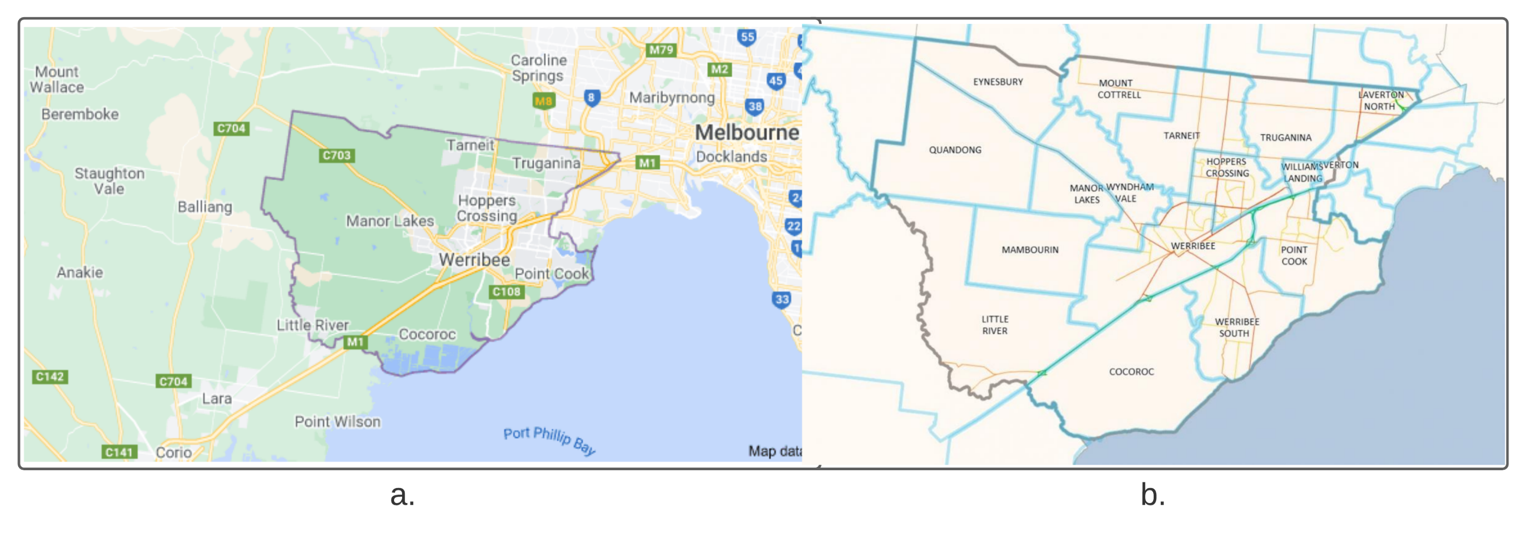
The Wyndham city council (VIC, Australia) area [13] was chosen as the study area, as shown in Figure 2. It is located on Melbourne’s western outskirts and covers an area of 542 km and has a coastmidrule of 27.4 km. It has an estimated resident population of 270,478, according to the 2019 census.
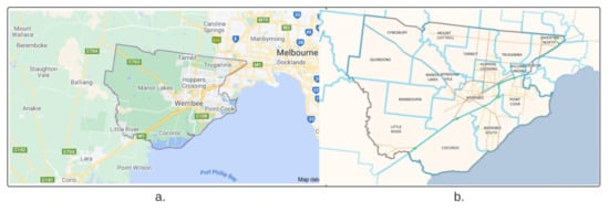
Figure 2.
(a) Location of the study area in Victoria, Australia. (b) Suburbs in the Wyndham city council.
Wyndham is currently the third fastest-growing local council in Victoria. Wyndham’s population is growing and diverse, and the community forecasts indicate the population will be more than 330,000 by 2031 [13]. There are 19 suburbs (Cocoroc, Eynesbury, Hoppers Crossing, Laverton North, Laverton RAAF, Little River, Mambourin, Mount Cottrell, Point Cook, Quandong, Tarneit, Truganina, Werribee, Werribee South, Williams Landing, Wyndham Vale) in Wyndham [58]. Wyndham City Council is committed to enhancing the environment and liveability of residents. As part of this commitment, thousands of new trees are planted each year to increase Wyndham’s tree canopy cover through the street tree planting program.
3.2. Google Street View (GSV) Imagery
The orientation of Eucalyptus trees (healthy and unhealthy) in a 360° GSV can be identified by GSV images. Images of the static street view have been downloaded via the GSV image application programming interface (API) [59] by supplying the corresponding parameter information with uniform resource locators (URLs) [60]. The GSV API snaps the requested coordinates automatically to the nearest GSV viewpoint. We have taken four GSV images with the fov of 90° and headings of 0°, 90°, 180°, 270°, respectively as shown in Figure 3.

Figure 3.
GSV images were obtained from 4 different viewpoints.
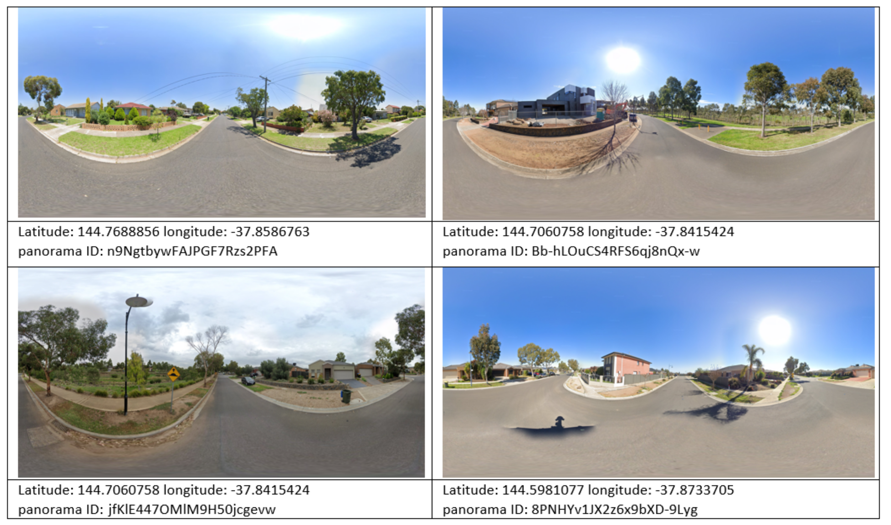
The “street-view” python package [61] was used for acquiring accurate latitude and longitude values for each GSV viewpoint to convert the coordinates requested to the nearest available Panorama IDs (i.e., unique panorama ID with purchased date [year, month], latitude and longitude). The latest Panorama ID was then used as the input location parameter as shown in Figure 4.
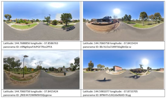
Figure 4.
Different location images of the study area with latitude, longitude values and panorama IDs.
We built a Python script to create the URLs and download 1000 GSV images to cover the study field automatically. To remove the Google logos, we cropped the downloaded images.
3.3. Annotation Data
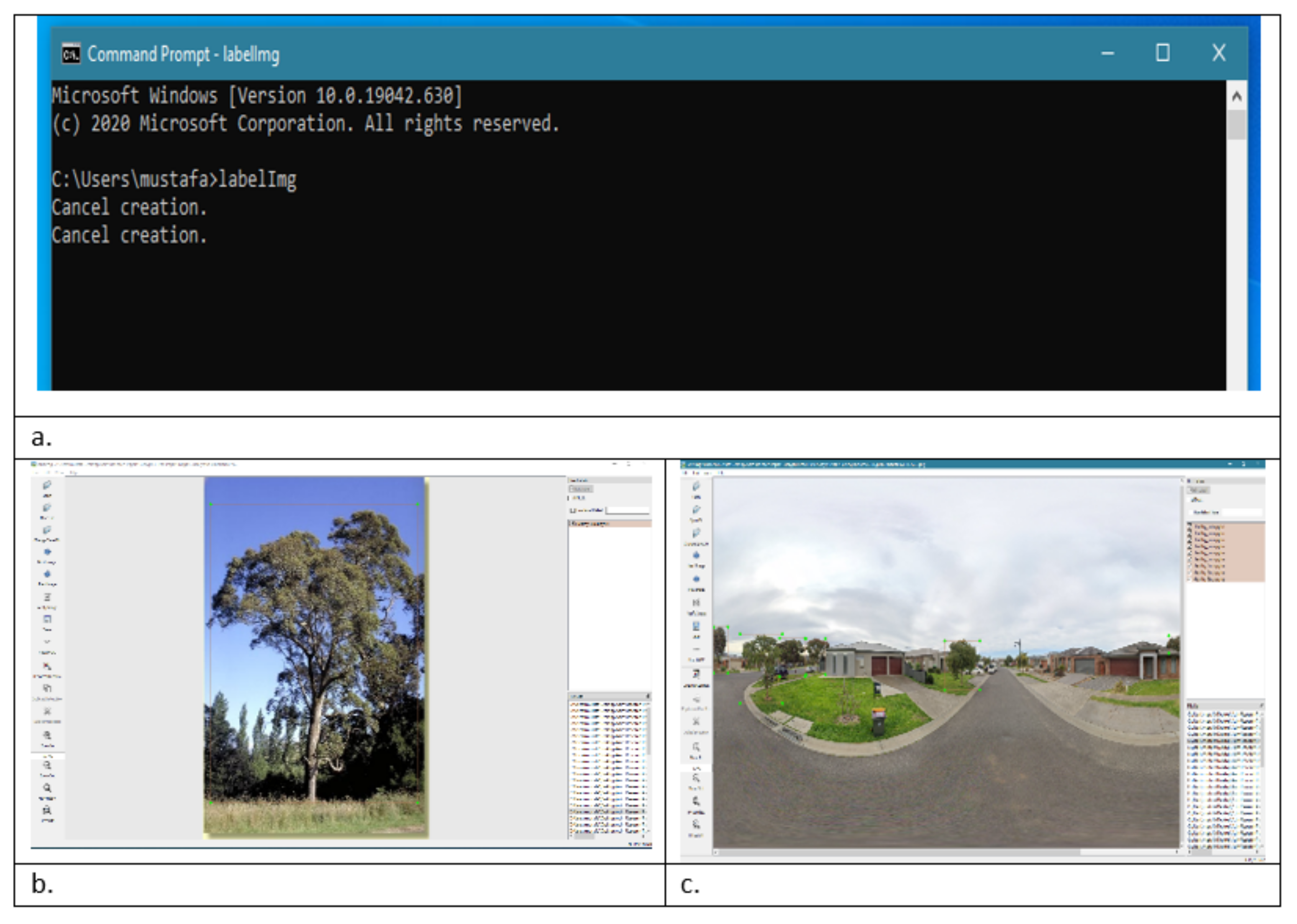
For deep supervised learning algorithms to be practical, large image data are essential. From GSV images acquired with screen captures on Google Maps, we created 1000 images data points by manually tagging Eucalyptus trees, as can be seen in Figure 5. To increase the methodology’s transferability, random Eucalyptus trees’ around 3500 images at the Wyndham city council, Victoria, Australia, were also taken for training, validation and testing of the model. We used “labelling” [62] for ground truth and panorama images. It is a tool written in Python for graphical image annotation and uses Qt for its graphical interface. Annotations are stored in PASCAL VOC, the format used by ImageNet, as XML files. We used the PASCAL VOC format because the Siamese network supports it. In DL, training an algorithm requires an ample training and validation dataset to minimise and prevent overfitting the model. At the same time, a test dataset is required to assess the trained model’s performance. In total, 4500 images from GSV and self-gathered images were annotated and used as a dataset for training, 500 for validation, and the other 500 for testing (accuracy) evaluation.

Figure 5.
(a) Command prompt-LabelmeImg screenshot, (b) Annotating single tree image, (c) Annotating panorama image.
3.4. Training Siamese CNN
We trained a Siamese CNN based on the central idea that if we use two input images from the same class, then their feature vectors must also be identical, and if two input images are not of the same class, then their feature vectors must also be different. Depending on the input image types, the vector features must be very different in these situations and the similarity score will also be different.
3.5. Siamese CNN Architecture
The word Siamese refers to twins [12]. Siamese Neural Network is a sub-class of neural network architecture that comprises of two or more networks [63]. These networks must be two copies of the same network, i.e., having the same configuration with the same parameters and weights.
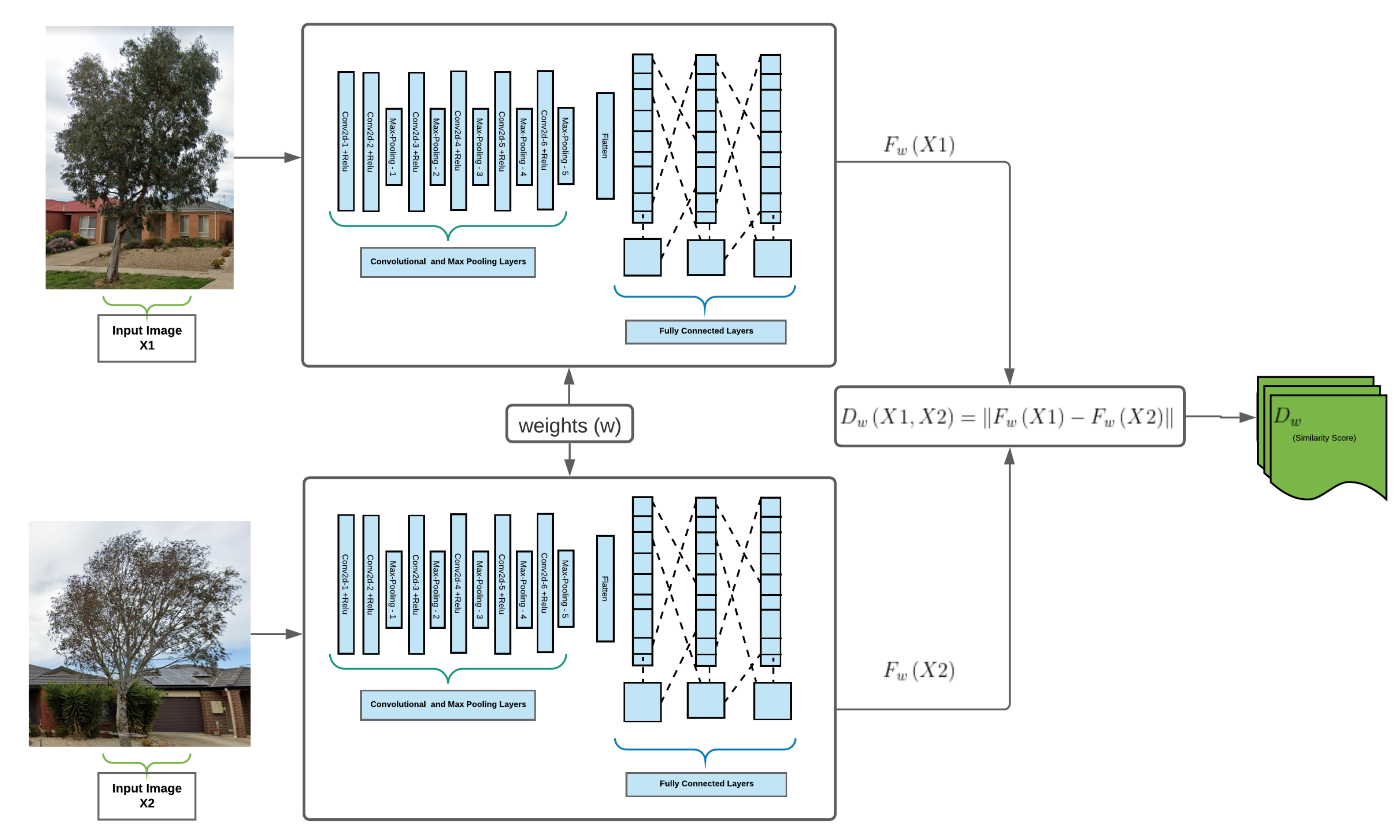
We used the Siamese network, consisting of two identical convolutional neural networks (CNN) [64]. The network architecture is the same as in our previous work [21], where an individual CNN is comprising of six convolutional layers and three fully connected or Dense layers. Each convolution layer contains two feature types, input and numeral filters. We used a 3 × 3 filter size for all convolution layers. The number of the filter is transformed into the next linked layer for each layer, which extracts the valuable features. One of the key benefits of the convolutional network is that the input image to the network can be much bigger than the size of the candidate image. Furthermore, in one evaluation, it will measure the similarity in all translated sub-windows on a dense grid. We search multiple scales in one forward-pass by assembling a mini-batch of scaled images. The output of this network performance is a score chart. For enhancing convergence speed, batch normalization [65] is applied to all convolutional layers except the last layer. We used five max-pooling layers that follow each convolutional layer to minimize the computational cost. The max-pooling has an active filter of 2 × 2 that slides on the input image and, based on the filter size; then the maximum value is selected as an output. The first two layers of the fully connected layers have ReLU activation [66] while the last layer (also known as the output layer) has a SoftMax activation [67]. The SoftMax activation finds the maximum probability value node and forwarded it as an output. A dropout of 0.5 is added to the fully connected layers to prevent over-fitting issues in the model. The total model parameters of our model are 51,161,305. Figure 6 is the visual representation of our Siamese network.

Figure 6.
Visual representation of Siamese network architecture that takes two different inputs and provides the inference.
3.5.1. Contrastive Loss Function
Features extracted by the subnetworks are fed into the decision-making network component, which determines the similarity. This decision-making network can be a loss function [68], i.e., contrastive loss function [69].
We trained Siamese CNN with contrastive loss function [69]. Contrastive loss is a distance-based loss function used to find embeddings where the Euclidean distance is small in two related points and high in two separate points [69]. Therefore, if input images are of same class, then loss function allows the network to output features close to feature space and if the input images are not similar then the output features are away. The similarity feature function is:
where and are the input images that shares the parameter vector w and , represents the input mapping in the feature space and Dw is the Euclidean distance. By calculating the Euclidean distance, Dw, between the feature vectors, the co-evolutionary Siamese network can be seen as a measuring function that measures the similarity between and .
We use contrastive loss function defined by Chopra et al. [70,71], in Siamese network training, defined as follows:
where y is a binary label assigned to input images and , y = 1 if both the inputs are of the same class and y = 0 if both inputs are of different class, while m > 0 is a margin value, must be chosen experimentally depending on the application domain.
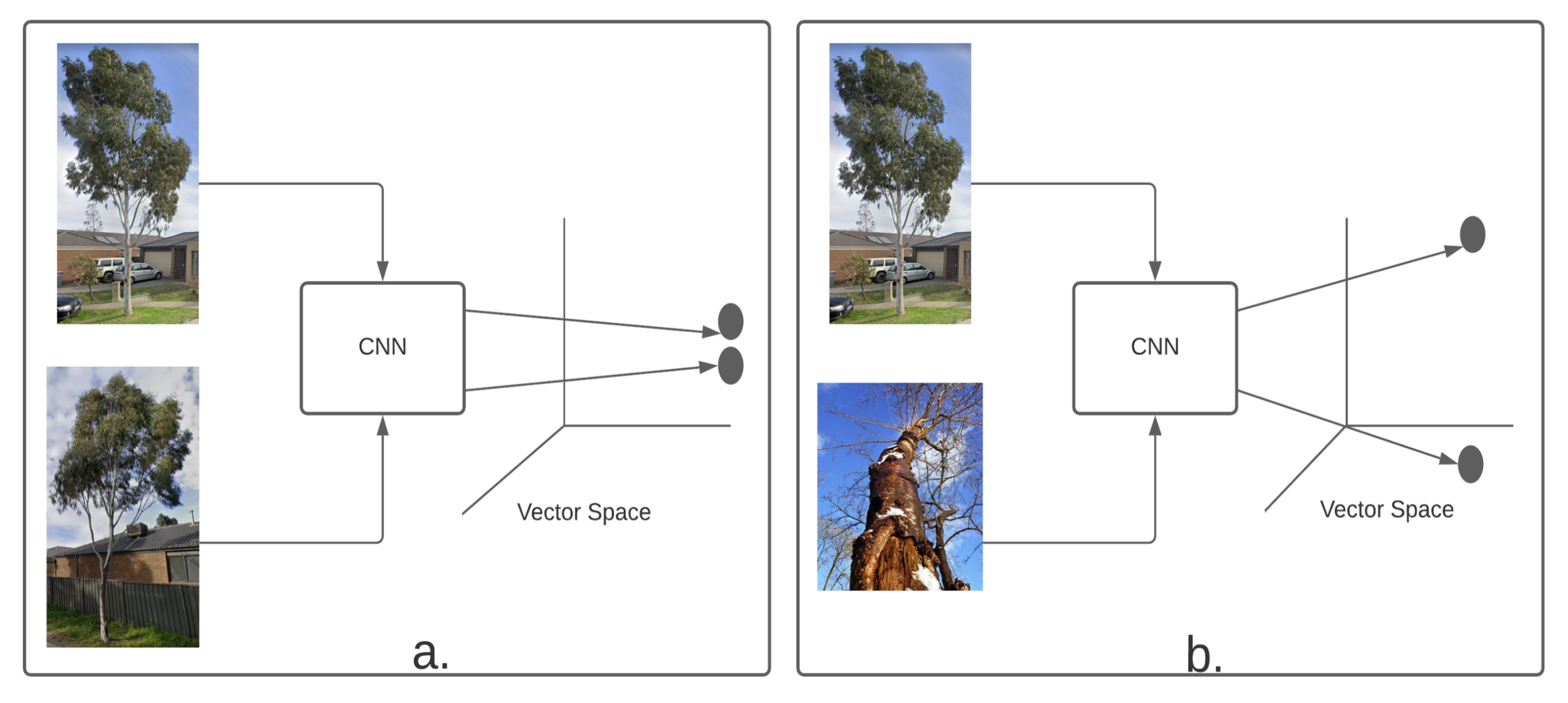
Minimizing with respect to w will then result in a small value of for images of the same species and a high value of for images of different species. This is visually represented in Figure 7.

Figure 7.
Contrastive loss function examples of (a) Positive (similar) and (b) Negative (different), images embedded into a vector space.
3.5.2. Mapping to Binary Function
A Siamese network takes an input of a pair of images, and the output is a similarity score. The similarity score will be 1 if both images belong to the same class, and it will be 0 if both input images are from different classes.
3.6. Geolocation Identification
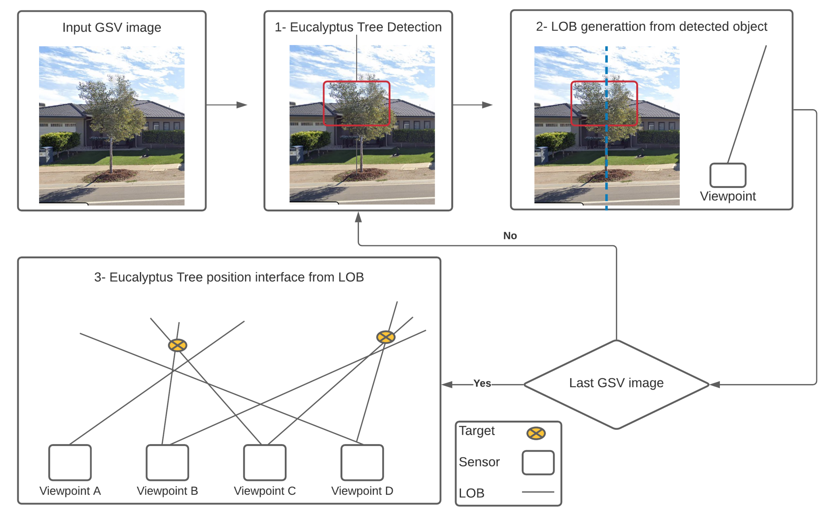
Our proposed DL-based automatic mapping method for Eucalyptus tree from GSV includes three main steps as shown in Figure 8. They are the following.
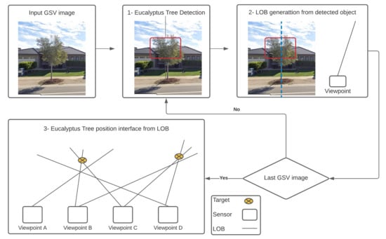
Figure 8.
The process of using deep learning to map Eucalyptus trees from GSV.
- Detect Eucalyptus tree in the GSV images using a trained DL network.
- Calculate the azimuth from each viewpoint to the detected Eucalyptus tree based on the known azimuth angles of the GSV images, relative to their view point locations, and the horizontal positions of the target in the images as shown in Figure 8 (2) using the mean value of two X values of the bounding box. For instance; suppose a detected Eucalyptus tree has a bounding box that is centered on column 228 in a GSV image that is centered at 0° azimuth relative to the image viewpoint. Each GSV image contains 640 columns and spans a 90° horizontal field-of-view; thus, each pixel spans 0.14. The center of the Eucalyptus tree is 130 pixels to the right of the image center (at column 320) and so has an azimuth of 18.2° relative to the image viewpoint. “Azimuth is an angle formed by a reference vector in a reference plane pointing towards (but not necessarily meeting) something of interest and a second vector in the same plane. For instance, With the sea as your reference plane, the Sun’s azimuth may be defined as the angle between due North and the point on the horizon where the Sun is currently visible. A hypothetical line drawn parallel to the sea’s surface could point in the Sun’s direction but never meet it.” [72].
- The final step is to estimate the target locations based on the azimuths calculated from the second step as presented in Figure 8 (3).
3.6.1. LOB Measurement Method
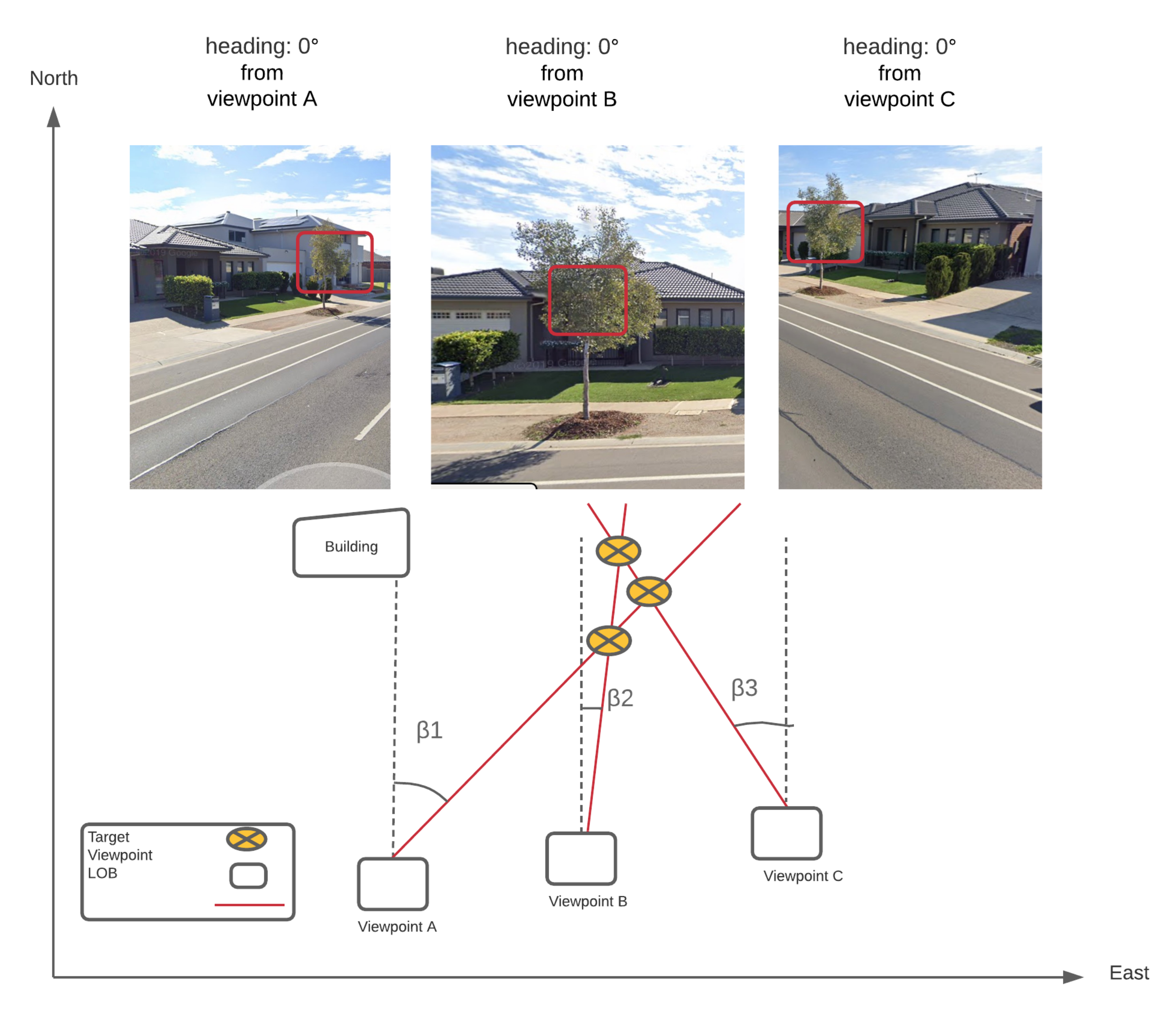
The bounding boxes of detected Eucalyptus trees, which result from the implementation of odometry from monocular vision of GSV images, are the outputs of Eucalyptus tree detection in GSV images using Siamese CNN, as shown in Figure 9. As a result, estimating Eucalyptus tree positions in pure GSV images is a multiple-source localization issue based on passive angle measurements that has been extensively studied [73,74]. One of three major multiple-source localization methods is the LOB-based method [75]. Since detected Eucalyptus tree are not signal sources such as propagating signal sources whose signal intensity can be calculated, a LOB calculation was used to estimate the position of a target Eucalyptus tree shown in Figure 9. Other methods (such as synchronization and power transit) necessitate more stringent requirements for a LOB calculation. Azimuths from multiple image viewpoints to a given Eucalyptus tree enable the Eucalyptus tree position to be triangulated in LOB localization presented in Figure 9. Since the LOB move through the target, the intersection of several LOB is ideally the exact location of the target as can be seen in Figure 9.
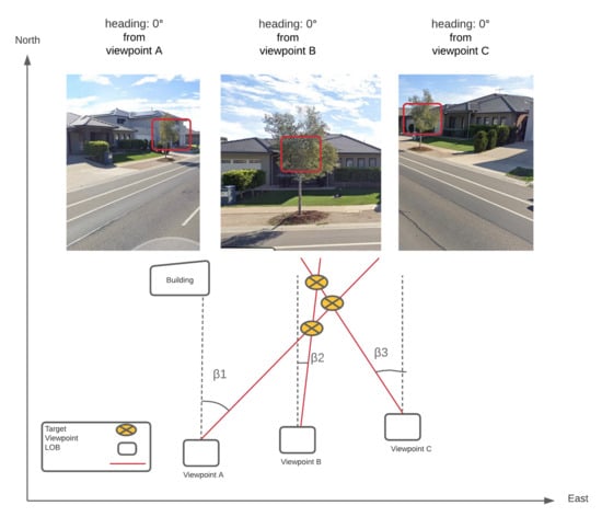
Figure 9.
An example of using bearing measurements to determine a target position from three different locations using a sensor.
When the LOB calculation is used in a dense emitter setting, however, many ghost nodes (i.e., false targets) appear, as shown in our study for estimating Eucalyptus tree locations in GSV images [76] as shown in Figure 10.
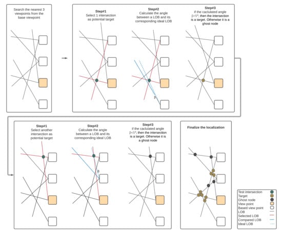
Figure 10.
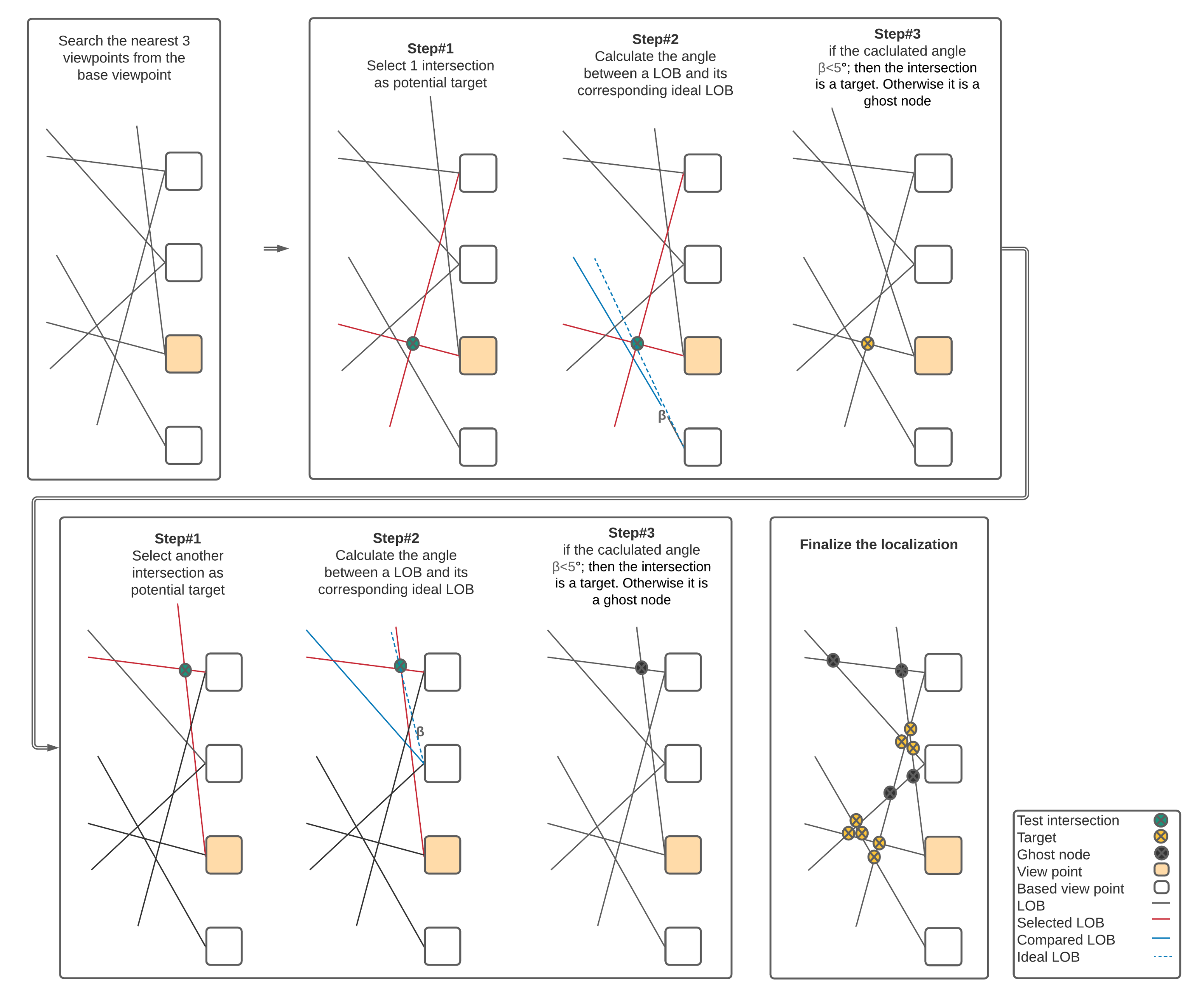
An example of how to use the brute-force-based three-station cross position algorithm to remove ghost nodes from four views with a 5° angle threshold.
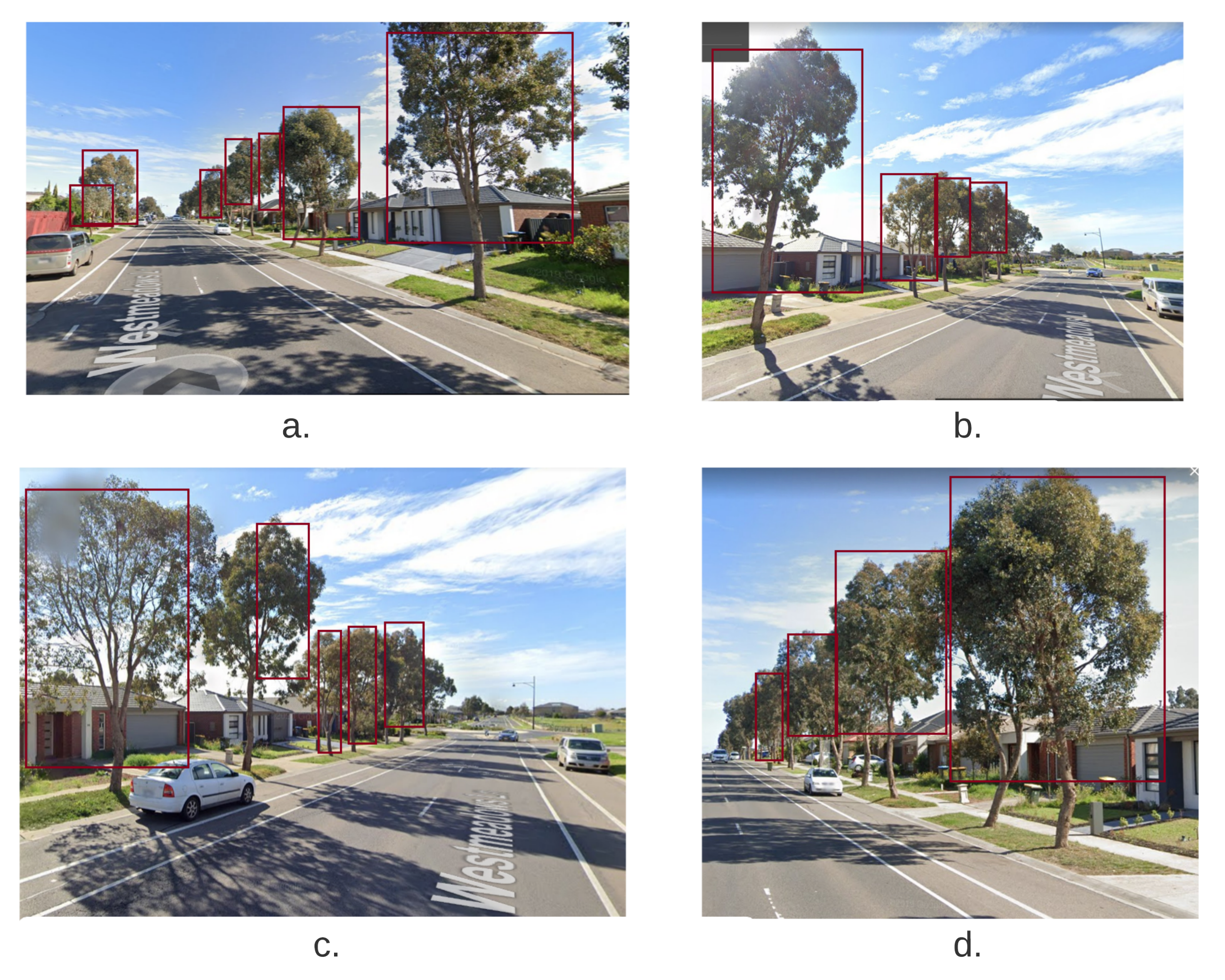
As a result, a modified brute-force-based three-station cross position algorithm was used to reduce the ghost node problem of multiple-source localization using LOB measurement as shown in Figure 11; source localization from viewpoints A, B, and C, based on two assumptions:
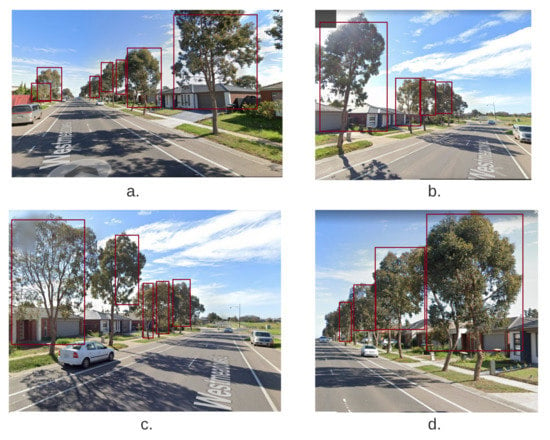
Figure 11.
Bounding boxes of labelled Eucalyptus tree in 4 GSV images (a–d).
- Targets and sensors are in the xy plane, and
- All LOB measurements are of equal precision [77].
The LOB measurement method shown in Figure 10 consists of the following steps:
- Find the closest neighboring viewpoints for a given viewpoint; we tested the algorithm’s performance using 2 to 8 of the closest neighboring viewpoints (i.e., the corresponding number of views is 3 to 9).
- Measure the angles between each pair of LOBs from all viewpoints [78].
- Check whether there are positive associations among LOBs (set at 50 m length) from current viewpoint and its neighboring viewpoints.
- Repeat the process from step 1 to step 3 for every intersection point.
To be more precise, a positive association among LOB is produced by three positive detections from any three views within an angle threshold () [77]. As a result, assuming constant detection rates, the number of predicted Eucalyptus trees increases as the number of views increases, based on the likelihood of combination. For example, suppose the total number of Eucalyptus trees estimation possibilities is t(t N); if the detection rate remains constant, the likelihood of a positive association with seven views (i.e., C(7, 3)/t) is greater than the probability of positive association with four views (i.e., C(4, 3)/t). To perform cross-validation in this analysis, the closest perspectives were chosen. A list of the nearest neighbouring perspectives (2, 3, 4, 5, 6, 7, and 8 viewpoints; that is 3, 4, 5, 6, 7, 8, and 9 views) and angle thresholds (1°, 2° and 3°) is used for testing to determine whether there is a positive correlation and which threshold functions better. Because of the span of the LOB and the interval between GSV acquisitions, only nine views were chosen for research (10 m). Eight perspectives are on a line on one side of the present perspective in the extreme case of nine views. For the intersection of two 50 m LOB, 80 m is almost the maximum distance needed.
3.6.2. Multiple LOB Intersection Points Aggregation
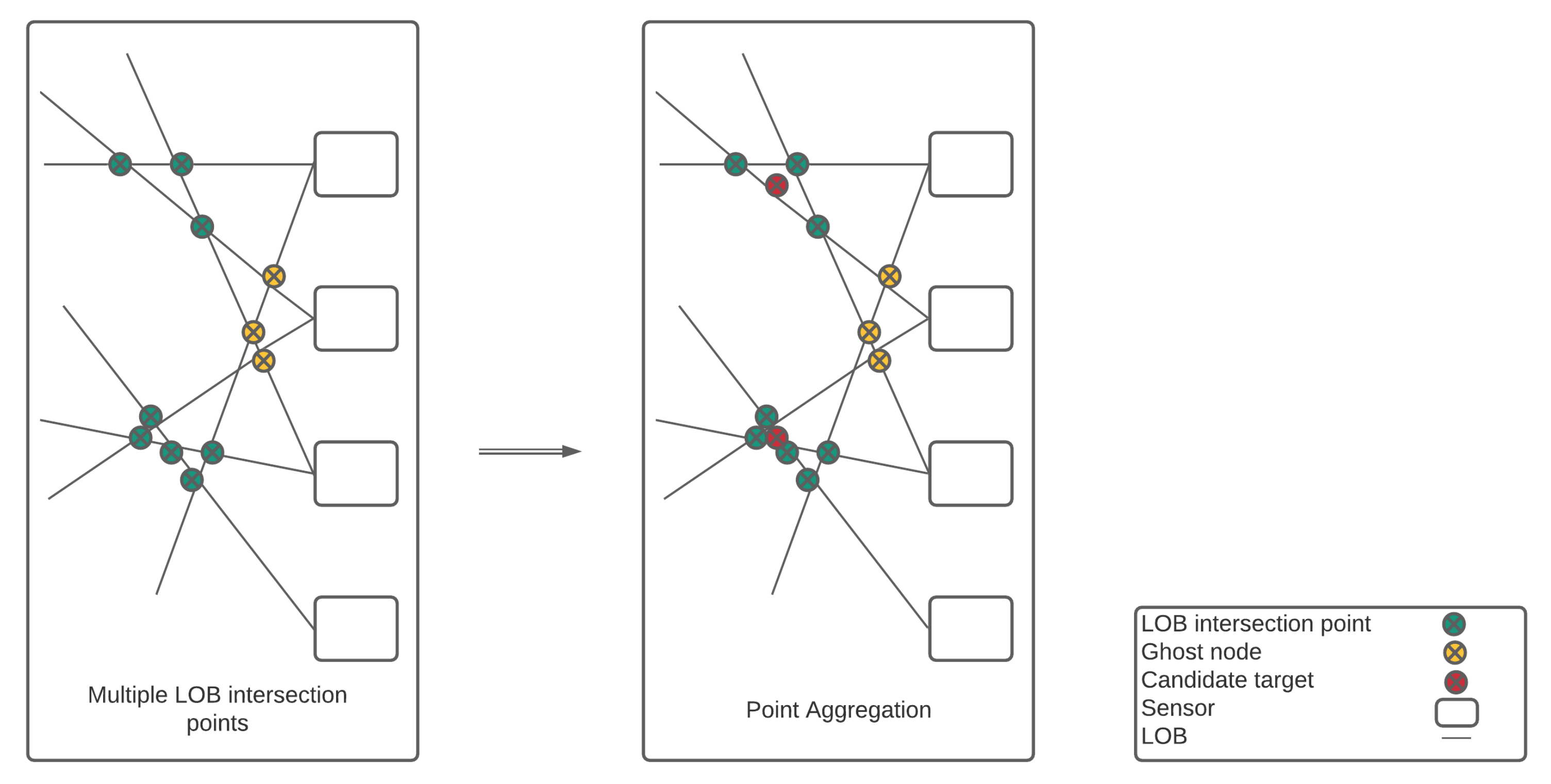
If we use a modified brute-force-based three-station cross-location algorithm, the result will be more than one LOB intersection point, and all these are possible targets for each Eucalyptus tree. To overcome this situation, we can further apply a geospatial algorithm, i.e., spatial aggregation (“Spatial Aggregation computes statistics in areas where an input layer and a boundary layer overlap” [79]) to determine where a Eucalyptus tree can be found. The primary purpose of this geospatial aggregation algorithm is to provide a central location (expected correct target) within a range of 10 m (this 10 m distance is given to the geospatial algorithm to apply aggregation on) of LOB intersection points. There are three main steps of this geospatial aggregation algorithm, as shown in Figure 12.
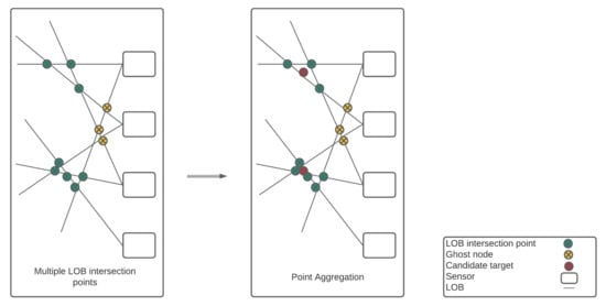
Figure 12.
An example of aggregating multiple LOB intersection points.
- Compute the Euclidean distance matrix between all LOB intersection points.
- The Euclidean distances between LOB intersection points are used to cluster LOB intersection points.
- Determine the centroid of each intersection point cluster.
3.6.3. Spatial Aggregation and Calculation of Points
Aggregation is the process of combining several objects with similar characteristics into a single entity, resulting in a less detailed layer than the original data. Aggregation, like any other type of generalization, removes some information (both spatial and attribute) but simplifies things for the consumer who is more interested in the unit as a whole rather than each individual component within it. Spatial aggregation [80] can be applied on Line, Points or Area; however, the calculation method is slightly different when calculating points. For Line and area features, average statistics are determined using a weighted mean. The following equation is used to calculate weighted mean [79].
where N = number of observations, = observations and = weights.
Only the point features inside the input boundary are used to summarise point layers. As a result, no equations are weighted. It must be ensured that all data from the same database link is stored in the same spatial reference system while performing spatial aggregation or spatial filtering [79,80].
4. Experiments and Results
4.1. Experiments
We implemented our experiments in Keras [81] backend TensorFlow [82]. Typically, any state-of-the-art architecture may be used as a backbone to extract the features. We performed our experiments with VGG-16 [83], AlexNet [84] and ResNet-34 [85] to explore how effective the backbone network is in extracting features. Siamese network consists of two sister/twin CNNs as both are two copies of the same network. They share the same parameters and network weights were initialized. The initial learning rate was set at 0.001 with an optimizer Stochastic Gradient Descent (SGD) [86], dropout was set to 0.5 and momentum 0.9. We used L2 Regularization to avoid over-fitting in the network [21]. All input images were resized into 100 × 100 before feeding into two identical networks in the Siamese network. The two input images of Eucalyptus trees ( and ) are passed through the networks and then through a fully connected layer to generate a feature vector for each () and (). We added a dense layer with ReLU activation and then finally an output layer with SoftMax activation.
4.2. System Configuration
All our experiments were performed on Intel Core i7-9700K CPU @ 3.60 GHz (8 cores and 8 threads), 32 GB RAM, NVidia Titan RTX 24GB VRAM GPU. For development and implementation of methodology, we used Python 3.8 and Keras-2.2 with Tensorflow-2.2.0 backend as the deep learning framework.
4.3. Approach
The entire dataset was split into 70% training, 10% validation and 20% test set. We applied various data augmentation techniques on the images and resized all images into 100 × 100 before feeding it into the Siamese network. The weights were initialized to avoid the layer activation from disappearing during the forward passage through a deep neural network [87]. We also used early stopping with a patience of 50 epochs.
4.4. Results
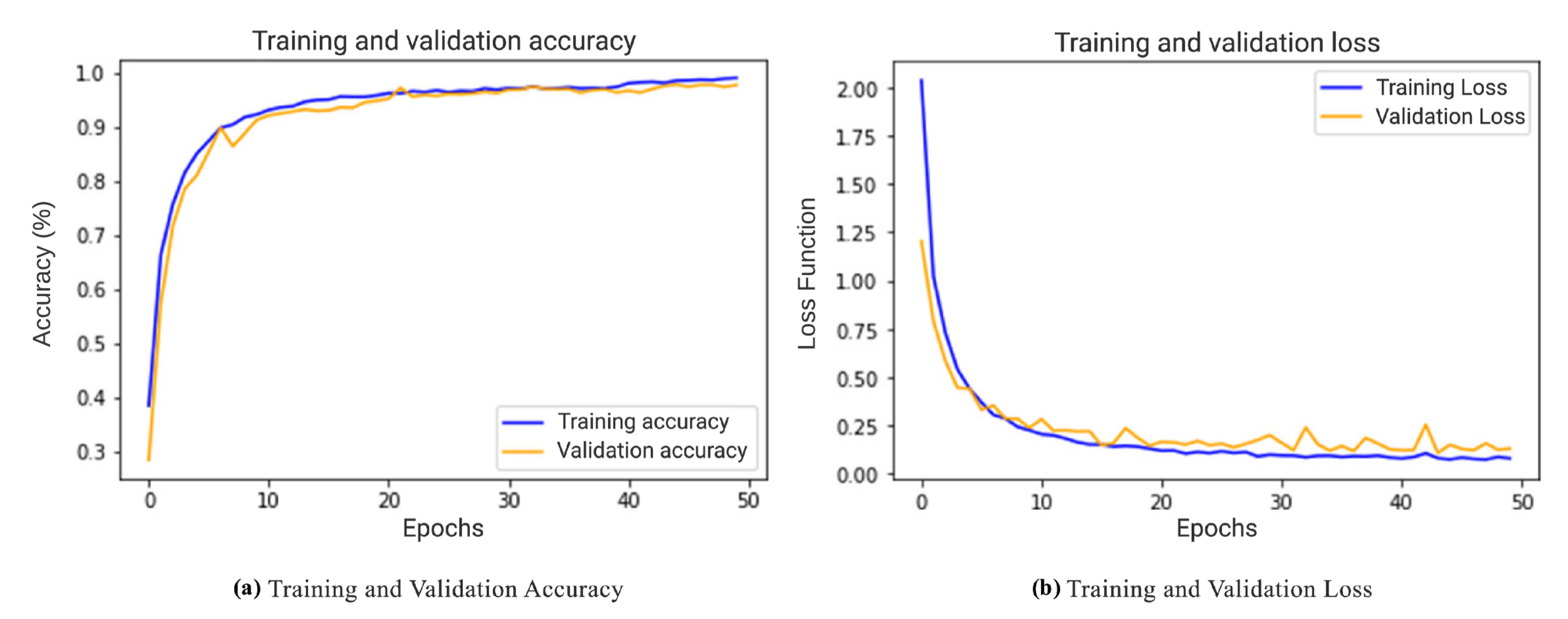
We used various networks such as VGG-16 [83], ResNet-34 [85], and AlexNet [84] in our experiments. While performing experiments, first, we froze a few layers in the backbone network and trained the network on the remaining layers that we added. The obtained results from the experiments with various networks were not satisfactory, i.e., 85.33%, 82.67% and 79.89%, respectively. The achieved results from the frozen layers were not satisfactory, so we unfroze all the layers and again performed the experiments to extract features for Eucalyptus trees input images. This time the results were 93.2%, 90.43% and 86.26%, respectively. In each experiment, a total of 50 epochs were conducted, where each epoch is the number of iterations. Finally, the Siamese network was trained at a batch size of 32 and stopped training on epoch-50 as shown in Figure 13.
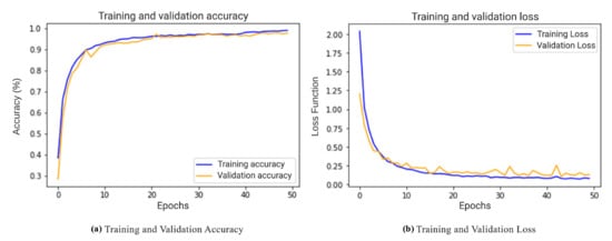
Figure 13.
Validating the object detection model learning.
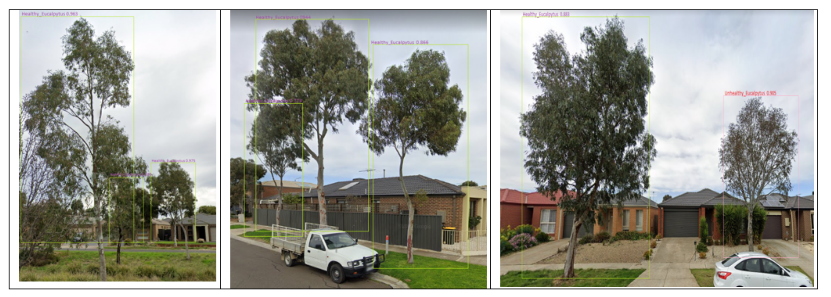
The initial experiments with VGG-16, ResNet-34, and AlexNet demonstrated that VGG-16 consistently produced the best results in our scenario, so we used it as the backbone for all of our experiments.The resulting features of VGG-16 experiments are transferred to the decision network to identify whether or not two input images are similar. A sample output is shown in Figure 14.
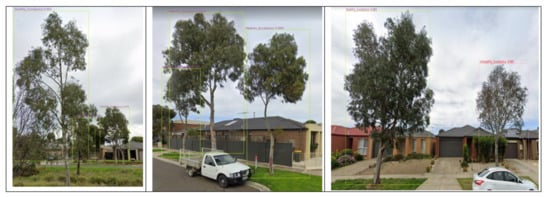
Figure 14.
Examples of identifying and classification of healthy and unhealthy Eucalyptus trees from GSV and ground truth images.
There are many methods of performance measurement that are used to evaluate the performance of neural networks. They include precision, recall, accuracy, and f1-score. Precision tells us about the correct predictions made out of false-positive while recall tells us about the correct predictions made out of false-negatives. The accuracy is the number of correct predictions out of both false-positives and false-negatives. We calculated all of our trained model’s performance metrics using the formulas in Equations (4)–(7) from the confusion matrix.
where TP is true positives, TN is true negatives, FP is false positives and FN is false negatives. Here the TP and TN are the correct predictions while the FP and FN are the wrong predictions made by our model. After computing values from the confusion matrix, the results are shown in Table 1.

Table 1.
Classification/Model Performance Report.
Location Estimation Accuracy Evaluation
The location estimation accuracy of the Eucalyptus tree is shown in Table 2 as a percentage of the number of predicted Eucalyptus tree positions within the buffer zones of a reference Eucalyptus tree. To assess the effects of the number of views, the angle threshold, and the distance to the middle of a chosen road, we considered seven views (i.e., 3, 4, 5, 6, 7, 8, 9), three angle thresholds (i.e., 1°, 2°, and 3°), and three distance thresholds to the centre of a selected road (i.e., 3 m, 4 m, and 5 m) to determine the impacts of the number of views, the angle threshold, and the distance threshold to the centre of a selected road. Around half of the estimated Eucalyptus tree locations were within the 6m buffer zone of their reference locations using the method we tested, and up to 79% of the estimated locations were within the 10 m buffer zone of their reference locations using the method we tested. However, about 12% of the approximate Eucalyptus tree positions were inside the 2 m reference position buffer zone.

Table 2.
Based on 1039 reference trees, the accuracy assessment of estimating position of Eucalyptus trees.
Table 2 reveals that using more views and higher angle thresholds resulted in a more approximate Eucalyptus tree in the modified brute-force-based three-station cross-location algorithm, which is due to the increased relaxation of the modified brute-force-based three-station cross-location algorithm. Meanwhile, because relaxation allows more ghost nodes to be estimated Eucalyptus trees, more estimated Eucalyptus trees may result in lower accuracy (see Table 2).
Table 2 shows that when comparing the results of other numbers of views, the average percentage of predicted Eucalyptus tree positions being inside all buffer zones of reference Eucalyptus trees for the results of eight views is the highest (47.80%). Using a greater distance to the centre of selected road thresholds, on the other hand, resulted in less approximate Eucalyptus trees. Since the optical GSV imagery was the only data source used to perform the localization, the precision of the position estimation for the Eucalyptus tree is fair, and the estimated data are helpful.
It is worth noting that GSV image distortion, terrain relief, GSV position accuracy, or limitations in the process we used may have caused location mismatches in some cases due to the ground positions of Eucalyptus trees varying from the orthographic predicted locations estimated from GSV images. For areas where GSV imagery is available and a Eucalyptus tree distribution map with a 10 m accuracy is appropriate, our proposed approach has a lot of promise. When a given Eucalyptus tree was not identified in at least three GSV images out of a certain number of views, our method failed to estimate the Eucalyptus tree’s location. Three is the minimum number of images needed to triangulate a position and remove ghost nodes (as can be seen in Figure 10). This explains why the number of projected Eucalyptus trees rises in tandem with the number of views (see Table 2).
5. Discussion
Eucalyptus trees are evergreen; however, an early sign that shows they are unhealthy is if they turn brown, either partially or completely. Various signs/aspects can be spotted in unhealthy Eucalyptus trees; one of the most apparent is the loss or decrease of leaf growth in all or parts of the tree. Other symptoms include the bark of the tree becoming brittle and peeling off, or the trunk of the tree becoming sponge-like or brittle. A tree may have bare branches, i.e., without leaves, in any season can be a sign of dead tree or branches that are loose and weak could indicate a dead or dying tree. Weak joints of Eucalyptus tree can be dangerous, as it means branches can come loose during bad weather [88]. If the whole Eucalyptus is dead, it can be left untouched for a period of maximum two years; however, after this, it becomes unsafe and needs to be removed.
Some of the common diseases in Eucalyptus [89] trees are shown in Figure 15a–c. It is critical to identify such unhealthy trees in order to improve the urban Eucalyptus tree’s health and environment.

Figure 15.
Some common diseases (a) Heart rot and (b) Phytophthora, and (c) Canker.
- a.
- Canker disease that infects the bark and then goes inside of the tree,
- b.
- Phytophthora disease goes directly under the bark by discolored leaves and dark brown wood, and
- c.
- The heart disease damages the tree from inside and outside.
Numerous approaches are studied in the current literature with regards to trees and their health in urban areas. Shendryk et al. [30] worked on the trunks of Eucalyptus trees, as well as their complex shapes. They used Euclidean distance clustering for individual tree trunk detection. Up to 67% of trees with diameters greater than or equal to 13 cm were successfully identified using their technique. Milto Miltiadou et al. [29] presented a new way to detect dead Eucalyptus camaldulensis with the introduction of DASOS (feature vector extraction). To do so, they attempted to research the odds of dead trees being detected using Voxel-based full-waveform (FW) LiDAR without tree demidruleation. It has been discovered that it is possible to determine tree health without outlining the trees, but since this is a new area of research, there are still many improvements to be made. Xiao et al. [47] presented that the trees were examined using remote sensing data and GIS techniques to examine their health. Trees had their conditions analysed in relation to physiognomy on two scales: the tree itself and in terms of pixels. A pixel-by-pixel analysis was performed in which each tree pixel within the tree crown was classified as either healthy or unhealthy based on values of vegetation index. A quantitative raster-based analysis was conducted on all of the trees, where they used the tree health index, which is a quantitative value that describes the number of healthy pixels compared to the total tree pixels on the crown. Classifying the tree as healthy if the index was greater than 70% of the overall index indicated that a random sample of 1186 trees was used to verify the accuracy of the tree data. When viewed at the whole tree level, approximately 86% of campus trees were found to be healthy and approximately 88% of mapping accuracy.
In contrast to the above-discussed literature, we propose a deep learning-based network, Siamese convolutional neural network (SCNN), combining a modified brute-force-base line-of-bearing (LOB) algorithm to classify Eucalyptus trees as healthy or unhealthy and to find their geolocation from the GSV and ground truth imagery. Our proposed method successfully achieved an average accuracy of 93.2% in identifying healthy and unhealthy trees and their geolocation. For training and validation of SCNN, a dataset of approximately 4500 images was used.
The main purpose of using Google imagery is that Google imagery is available publicly online and no privately man laboured efforts are required in order to capture the images. Second, using of sentinel imagery would be an expensive option and time consuming solution, as the sentinel’s imagery requires longer time period to obtain images of specific locations and needs to subscribe to pay for receiving the service; i.e., it is not publicly available. The sentinel imagery is also protected by copyright. Therefore, in this work, we used GSV and ground truth image for obtaining better results and overcome the some of the challenges as discribed in the Introduction Section. It is worth mentioning that “the satellite data on Google Maps is typically between 1 to 3 years old”. According to the Google Earth and other sources, data updates usually about once a month, but they may not show real-time images. Google Earth gathers data from various satellite and aerial photography sources, and it can take months to process, compare and set up the data before it appears on a map. However, in some circumstances, Google Maps are updated in real time to mark major events and to provide assistance in emergency situations. For example, it updated imagery for the 2012 London Olympic Games just before the Opening Ceremony, and it provided updated satellite crisis maps to help aid teams assess damage and target locations in need of help shortly after the Nepal earthquake in April 2015 [90,91].
6. Conclusions, Limitations, and Future Directions
Identifying various healthy and unhealthy Eucalyptus trees using traditional and manual methods is time-consuming and labor-intensive. This study is primarily an exploratory one that employs a DL-based method for identification, classification, and geolocation estimation. In this study, we present a Siamese CNN (SCNN) architecture trained to identify and classify healthy and unhealthy Eucalyptus trees and their geographical location. The SCNN uses the contrastive loss function to calculate its similarity score from two input images (one for each CNN). With the large number of GSV images available online, the method could be a useful tool for automatically mapping healthy and unhealthy Eucalyptus trees, as well as mapping their geolocation on metropolitan streets and roads. Although the model correctly identifies the Eucalyptus tree’s health status and position, is certainly worth mentioning some limitations to consider. First, it is still challenging to map up-to-date GSV images with geographical location information because the changing nature of imagery is rapid. Secondly, to achieve reasonable accuracy for geolocation with the DL, a large amount of training data is needed. Thirdly, when Eucalyptus trees have a big lean, the LOB method requires more attention; this is due to terrain and GSV’s visual distortion without compensation. Finally, the method suggested that automatic tree geolocation recognition can be useful, and in a future study it might be used to detect and classify other objects along the roadside.
Author Contributions
Conceptualization, A.K.; Methodology, A.K.; Software, A.K.; Validation, A.K. and B.G.; Formal analysis, A.K.; Investigation, A.K. and W.A.; Resources, A.K.; Data curation, A.K. and W.A.; Writing—original draft preparation, A.K.; Writing—review and editing, A.K., B.G., W.A., A.U. and R.W.R.; Visualization, A.K., B.G. and W.A.; Supervision, A.U. and R.W.R.; Project administration, A.K., A.U. and R.W.R.; Funding acquisition, A.U. and R.W.R. All authors have read and agreed to the published version of the manuscript.
Funding
This study received no external funding. However, Victoria University, Footscray 3011, Australia and Charles Sturt University, Port Macquarie (Campus), NSW 2444, Australia, equally funded.
Institutional Review Board Statement
Not applicable.
Informed Consent Statement
Not applicable.
Data Availability Statement
The data used to support the findings of this study are available from the corresponding author upon request.
Conflicts of Interest
The authors declare no conflict of interest.
References
- Branson, S.; Wegner, J.D.; Hall, D.; Lang, N.; Schindler, K.; Perona, P. From Google Maps to a fine-grained catalog of street trees. ISPRS J. Photogramm. Remote Sens. 2018, 135, 13–30. [Google Scholar] [CrossRef]
- Salmond, J.A.; Tadaki, M.; Vardoulakis, S.; Arbuthnott, K.; Coutts, A.; Demuzere, M.; Dirks, K.N.; Heaviside, C.; Lim, S.; Macintyre, H.; et al. Health and climate related ecosystem services provided by street trees in the urban environment. Environ. Health 2016, 15, 95–111. [Google Scholar] [CrossRef] [PubMed]
- Ladiges, P. The Story of Our Eucalypts—Curious. Available online: https://www.science.org.au/curious/earth-environment/story-our-eucalypts (accessed on 4 January 2021).
- Eucalypt Forest—Department of Agriculture. Available online: https://www.agriculture.gov.au/abares/forestsaustralia/profiles/eucalypt-2016 (accessed on 4 January 2021).
- Berrang, P.; Karnosky, D.F.; Stanton, B.J. Environmental factors affecting tree health in New York City. J. Arboric. 1985, 11, 185–189. [Google Scholar]
- Cregg, B.M.; Dix, M.E. Tree moisture stress and insect damage in urban areas in relation to heat island effects. J. Arboric. 2001, 27, 8–17. [Google Scholar]
- Winn, M.F.; Lee, S.M.; Araman, P.A. Urban tree crown health assessment system: A tool for communities and citizen foresters. In Proceedings of the Proceedings, Emerging Issues Along Urban-Rural Interfaces II: Linking Land-Use Science and Society, Atlanta, GA, USA, 9–12 April 2007; pp. 180–183. [Google Scholar]
- Czerniawska-Kusza, I.; Kusza, G.; Dużyński, M. Effect of deicing salts on urban soils and health status of roadside trees in the Opole region. Environ. Toxicol. Int. J. 2004, 19, 296–301. [Google Scholar] [CrossRef]
- Day, S.D.; Bassuk, N.L. A review of the effects of soil compaction and amelioration treatments on landscape trees. J. Arboric. 1994, 20, 9–17. [Google Scholar]
- Doody, T.; Overton, I. Environmental management of riparian tree health in the Murray-Darling Basin, Australia. River Basin Manag. V 2009, 124, 197. [Google Scholar]
- Butt, N.; Pollock, L.J.; McAlpine, C.A. Eucalypts face increasing climate stress. Ecol. Evol. 2013, 3, 5011–5022. [Google Scholar] [CrossRef]
- Chicco, D. Siamese neural networks: An overview. Artificial Neural Networks; Springer: New York, NY, USA, 2021; pp. 73–94. [Google Scholar]
- About Us—Wyndham City. Available online: https://www.wyndham.vic.gov.au/about-us (accessed on 4 January 2021).
- Google Street View Imagery—Google Search. Available online: https://www.google.com/search?q=google+street+view+imagery&rlz=1C1CHBF_en-GBAU926AU926&oq=google+&aqs=chrome.1.69i57j35i39l2j69i60l2j69i65j69i60l2.7725j0j4&sourceid=chrome&ie=UTF-8 (accessed on 4 January 2021).
- Anguelov, D.; Dulong, C.; Filip, D.; Frueh, C.; Lafon, S.; Lyon, R.; Ogale, A.; Vincent, L.; Weaver, J. Google street view: Capturing the world at street level. Computer 2010, 43, 32–38. [Google Scholar] [CrossRef]
- Li, X.; Zhang, C.; Li, W.; Ricard, R.; Meng, Q.; Zhang, W. Assessing street-level urban greenery using Google Street View and a modified green view index. Urban For. Urban Green. 2015, 14, 675–685. [Google Scholar] [CrossRef]
- Li, X.; Zhang, C.; Li, W.; Kuzovkina, Y.A.; Weiner, D. Who lives in greener neighborhoods? The distribution of street greenery and its association with residents’ socioeconomic conditions in Hartford, Connecticut, USA. Urban For. Urban Green. 2015, 14, 751–759. [Google Scholar] [CrossRef]
- Li, X.; Zhang, C.; Li, W. Building block level urban land-use information retrieval based on Google Street View images. GIScience Remote Sens. 2017, 54, 819. [Google Scholar] [CrossRef]
- Zhang, W.; Li, W.; Zhang, C.; Hanink, D.M.; Li, X.; Wang, W. Parcel-based urban land use classification in megacity using airborne LiDAR, high resolution orthoimagery, and Google Street View. Comput. Environ. Urban Syst. 2017, 64, 215–228. [Google Scholar] [CrossRef]
- Li, X.; Ratti, C.; Seiferling, I. Quantifying the shade provision of street trees in urban landscape: A case study in Boston, USA, using Google Street View. Landsc. Urban Plan. 2018, 169, 81–91. [Google Scholar] [CrossRef]
- Khan, A.; Nawaz, U.; Ulhaq, A.; Robinson, R.W. Real-time plant health assessment via implementing cloud-based scalable transfer learning on AWS DeepLens. PLoS ONE 2020, 15. [Google Scholar] [CrossRef]
- Khan, A.; Ulhaq, A.; Robinson, R.; Ur Rehman, M. Detection of Vegetation in Environmental Repeat Photography: A New Algorithmic Approach in Data Science; Statistics for Data Science and Policy Analysis; Rahman, A., Ed.; Springer: Singapore, 2020; pp. 145–157. [Google Scholar]
- Tumas, P.; Nowosielski, A.; Serackis, A. Pedestrian detection in severe weather conditions. IEEE Access 2020, 8, 62775–62784. [Google Scholar] [CrossRef]
- Guo, G.; Wang, H.; Yan, Y.; Zheng, J.; Li, B. A fast face detection method via convolutional neural network. Neurocomputing 2020, 395, 128–137. [Google Scholar] [CrossRef]
- Wu, J.; Song, L.; Wang, T.; Zhang, Q.; Yuan, J. Forest r-cnn: Large-vocabulary long-tailed object detection and instance segmentation. In Proceedings of the 28th ACM International Conference on Multimedia, Seattle, WA, USA, 12–16 October 2020; pp. 1570–1578. [Google Scholar]
- Islam, M.M.; Yang, H.C.; Poly, T.N.; Jian, W.S.; Li, Y.C.J. Deep learning algorithms for detection of diabetic retinopathy in retinal fundus photographs: A systematic review and meta-analysis. Comput. Methods Programs Biomed. 2020, 191, 105320. [Google Scholar] [CrossRef]
- Zeng, D.; Yu, F. Research on the Application of Big Data Automatic Search and Data Mining Based on Remote Sensing Technology. In Proceedings of the 2020 3rd International Conference on Artificial Intelligence and Big Data (ICAIBD), Chengdu, China, 28–31 May 2020; pp. 122–127. [Google Scholar]
- Voulodimos, A.; Doulamis, N.; Doulamis, A.; Protopapadakis, E. Deep learning for computer vision: A brief review. Comput. Intell. Neurosci. 2018, 2018, 7068349. [Google Scholar] [CrossRef]
- Miltiadou, M.; Campbell, N.D.; Aracil, S.G.; Brown, T.; Grant, M.G. Detection of dead standing Eucalyptus camaldulensis without tree delineation for managing biodiversity in native Australian forest. Int. J. Appl. Earth Obs. Geoinf. 2018, 67, 135–147. [Google Scholar] [CrossRef]
- Shendryk, I.; Broich, M.; Tulbure, M.G.; Alexandrov, S.V. Bottom-up delineation of individual trees from full-waveform airborne laser scans in a structurally complex eucalypt forest. Remote Sens. Environ. 2016, 173, 69–83. [Google Scholar] [CrossRef]
- Kamińska, A.; Lisiewicz, M.; Stereńczak, K.; Kraszewski, B.; Sadkowski, R. Species-related single dead tree detection using multi-temporal ALS data and CIR imagery. Remote Sens. Environ. 2018, 219, 31–43. [Google Scholar] [CrossRef]
- Weinmann, M.; Weinmann, M.; Mallet, C.; Brédif, M. A classification-segmentation framework for the detection of individual trees in dense MMS point cloud data acquired in urban areas. Remote Sens. 2017, 9, 277. [Google Scholar] [CrossRef]
- Briechle, S.; Krzystek, P.; Vosselman, G. Classification of tree species and standing dead trees by fusing UAV-based lidar data and multispectral imagery in the 3D deep neural network PointNet++. ISPRS Ann. Photogramm. Remote Sens. Spat. Inf. Sci. 2020, 5, 203–210. [Google Scholar] [CrossRef]
- Mollaei, Y.; Karamshahi, A.; Erfanifard, S. Detection of the Dry Trees Result of Oak Borer Beetle Attack Using Worldview-2 Satellite and UAV Imagery an Object-Oriented Approach. J Remote Sens. GIS 2018, 7, 2. [Google Scholar] [CrossRef]
- Yao, W.; Krzystek, P.; Heurich, M. Identifying standing dead trees in forest areas based on 3D single tree detection from full waveform lidar data. ISPRS Ann. Protogrammetry, Remote Sens. Spat. Inf. Sci. 2012, 1, 7. [Google Scholar] [CrossRef]
- Deng, X.; Lan, Y.; Hong, T.; Chen, J. Citrus greening detection using visible spectrum imaging and C-SVC. Comput. Electron. Agric. 2016, 130, 177–183. [Google Scholar] [CrossRef]
- Lan, Y.; Huang, Z.; Deng, X.; Zhu, Z.; Huang, H.; Zheng, Z.; Lian, B.; Zeng, G.; Tong, Z. Comparison of machine learning methods for citrus greening detection on UAV multispectral images. Comput. Electron. Agric. 2020, 171, 105234. [Google Scholar] [CrossRef]
- Shendryk, I.; Broich, M.; Tulbure, M.G.; McGrath, A.; Keith, D.; Alexandrov, S.V. Mapping individual tree health using full-waveform airborne laser scans and imaging spectroscopy: A case study for a floodplain eucalypt forest. Remote Sens. Environ. 2016, 187, 202–217. [Google Scholar] [CrossRef]
- Meng, R.; Dennison, P.E.; Zhao, F.; Shendryk, I.; Rickert, A.; Hanavan, R.P.; Cook, B.D.; Serbin, S.P. Mapping canopy defoliation by herbivorous insects at the individual tree level using bi-temporal airborne imaging spectroscopy and LiDAR measurements. Remote Sens. Environ. 2018, 215, 170–183. [Google Scholar] [CrossRef]
- López-López, M.; Calderón, R.; González-Dugo, V.; Zarco-Tejada, P.J.; Fereres, E. Early detection and quantification of almond red leaf blotch using high-resolution hyperspectral and thermal imagery. Remote Sens. 2016, 8, 276. [Google Scholar] [CrossRef]
- Barnes, C.; Balzter, H.; Barrett, K.; Eddy, J.; Milner, S.; Suárez, J.C. Airborne laser scanning and tree crown fragmentation metrics for the assessment of Phytophthora ramorum infected larch forest stands. For. Ecol. Manag. 2017, 404, 294–305. [Google Scholar] [CrossRef]
- Fassnacht, F.E.; Latifi, H.; Ghosh, A.; Joshi, P.K.; Koch, B. Assessing the potential of hyperspectral imagery to map bark beetle-induced tree mortality. Remote Sens. Environ. 2014, 140, 533–548. [Google Scholar] [CrossRef]
- Chi, D.; Degerickx, J.; Yu, K.; Somers, B. Urban Tree Health Classification Across Tree Species by Combining Airborne Laser Scanning and Imaging Spectroscopy. Remote Sens. 2020, 12, 2435. [Google Scholar] [CrossRef]
- Näsi, R.; Honkavaara, E.; Lyytikäinen-Saarenmaa, P.; Blomqvist, M.; Litkey, P.; Hakala, T.; Viljanen, N.; Kantola, T.; Tanhuanpää, T.; Holopainen, M. Using UAV-based photogrammetry and hyperspectral imaging for mapping bark beetle damage at tree-level. Remote Sens. 2015, 7, 15467–15493. [Google Scholar] [CrossRef]
- Näsi, R.; Honkavaara, E.; Blomqvist, M.; Lyytikäinen-Saarenmaa, P.; Hakala, T.; Viljanen, N.; Kantola, T.; Holopainen, M. Remote sensing of bark beetle damage in urban forests at individual tree level using a novel hyperspectral camera from UAV and aircraft. Urban For. Urban Green. 2018, 30, 72–83. [Google Scholar] [CrossRef]
- Degerickx, J.; Roberts, D.A.; McFadden, J.P.; Hermy, M.; Somers, B. Urban tree health assessment using airborne hyperspectral and LiDAR imagery. Int. J. Appl. Earth Obs. Geoinf. 2018, 73, 26–38. [Google Scholar] [CrossRef]
- Xiao, Q.; McPherson, E.G. Tree health mapping with multispectral remote sensing data at UC Davis, California. Urban Ecosyst. 2005, 8, 349–361. [Google Scholar] [CrossRef]
- Goldbergs, G.; Maier, S.W.; Levick, S.R.; Edwards, A. Efficiency of individual tree detection approaches based on light-weight and low-cost UAS imagery in Australian Savannas. Remote Sens. 2018, 10, 161. [Google Scholar] [CrossRef]
- Fassnacht, F.E.; Mangold, D.; Schäfer, J.; Immitzer, M.; Kattenborn, T.; Koch, B.; Latifi, H. Estimating stand density, biomass and tree species from very high resolution stereo-imagery – towards an all-in-one sensor for forestry applications? For. Int. J. For. Res. 2017, 90, 613–631. [Google Scholar] [CrossRef]
- Li, W.; He, C.; Fu, H.; Zheng, J.; Dong, R.; Xia, M.; Yu, L.; Luk, W. A Real-Time Tree Crown Detection Approach for Large-Scale Remote Sensing Images on FPGAs. Remote Sens. 2019, 11, 1025. [Google Scholar] [CrossRef]
- Ruiz, V.; Linares, I.; Sanchez, A.; Velez, J.F. Off-line handwritten signature verification using compositional synthetic generation of signatures and Siamese Neural Networks. Neurocomputing 2020, 374, 30–41. [Google Scholar] [CrossRef]
- Zhao, X.; Zhou, S.; Lei, L.; Deng, Z. Siamese network for object tracking in aerial video. In Proceedings of the 2018 IEEE 3rd International Conference on Image, Vision and Computing (ICIVC), Chongqing, China, 27–29 June 2018; pp. 519–523. [Google Scholar]
- Rao, D.J.; Mittal, S.; Ritika, S. Siamese Neural Networks for One-Shot Detection of Railway Track Switches. Available online: https://arxiv.org/abs/1712.08036 (accessed on 21 December 2017).
- Chandra, M.; Redkar, S.; Roy, S.; Patil, P. Classification of Various Plant Diseases Using Deep Siamese Network. Available online: https://www.researchgate.net/profile/Manish-Chandra-3/publication/341322315_CLASSIFICATION_OF_VARIOUS_PLANT_DISEASES_USING_DEEP_SIAMESE_NETWORK/links/5ebaa82f299bf1c09ab52e48/CLASSIFICATION-OF-VARIOUS-PLANT-DISEASES-USING-DEEP-SIAMESE-NETWORK.pdf (accessed on 12 May 2020).
- Shorfuzzaman, M.; Hossain, M.S. MetaCOVID: A Siamese neural network framework with contrastive loss for n-shot diagnosis of COVID-19 patients. Pattern Recognit. 2020, 113, 107700. [Google Scholar] [CrossRef]
- Bromley, J.; Bentz, J.W.; Bottou, L.; Guyon, I.; Lecun, Y.; Moore, C.; Säckinger, E.; Shah, R. Signature Verification Using a “Siamese” Time Delay Neural Network. Int. J. Pattern Recognit. Artif. Intell. 1993, 07, 669–688. [Google Scholar] [CrossRef]
- Wang, B.; Wang, D. Plant Leaves Classification: A Few-Shot Learning Method Based on Siamese Network. IEEE Access 2019, 7, 27008–27016. [Google Scholar] [CrossRef]
- Wyndham City Suburbs | Wyndham City Advocacy. Available online: https://wyndham-digital.iconagency.com.au/node/10 (accessed on 4 January 2021).
- What Is an Application Programming Interface (API)? | IBM. Available online: https://www.ibm.com/cloud/learn/api (accessed on 4 January 2021).
- Berners-Lee, T.; Masinter, L.; McCahill, M. Uniform Resource Locators. 1994. Available online: https://dl.acm.org/doi/book/10.17487/RFC1738 (accessed on 28 May 2021).
- GitHub-Robolyst/Streetview: Python Module for Retrieving Current and Historical Photos from Google Street View. Available online: https://github.com/robolyst/streetview (accessed on 1 April 2021).
- GitHub-Tzutalin/labelImg: LabelImg Is a Graphical Image Annotation Tool and Label Object Bounding Boxes in Images. Available online: https://github.com/tzutalin/labelImg (accessed on 1 April 2021).
- A Friendly Introduction to Siamese Networks | by Sean Benhur J | Towards Data Science. Available online: https://towardsdatascience.com/a-friendly-introduction-to-siamese-networks-85ab17522942 (accessed on 1 April 2021).
- Zhang, K.; Zuo, W.; Gu, S.; Zhang, L. Learning deep CNN denoiser prior for image restoration. In Proceedings of the IEEE Conference on Computer Vision and Pattern Recognition, Honolulu, HI, USA, 21–26 July 2017; pp. 3929–3938. [Google Scholar]
- Santurkar, S.; Tsipras, D.; Ilyas, A.; Madry, A. How does batch normalization help optimization? In Proceedings of the Advances in Neural Information Processing Systems, Montréal, QC, Canada, 2–8 December 2018; pp. 2483–2493. [Google Scholar]
- Li, Y.; Yuan, Y. Convergence analysis of two-layer neural networks with relu activation. In Proceedings of the Advances in Neural Information Processing Systems, Long Beach, CA, 4–9 December 2017; pp. 597–607. [Google Scholar]
- Dunne, R.A.; Campbell, N.A. On the Pairing of the Softmax Activation and Cross-Entropy Penalty Functions and the Derivation of the Softmax Activation Function. Available online: https://citeseerx.ist.psu.edu/viewdoc/download?doi=10.1.1.49.6403&rep=rep1&type=pdf (accessed on 28 May 2021).
- Nassar, A.S.; Lefèvre, S.; Wegner, J.D. Multi-View Instance Matching with Learned Geometric Soft-Constraints. ISPRS Int. J. Geo-Inf. 2020, 9, 687. [Google Scholar] [CrossRef]
- Contrastive Loss Explained. Contrastive Loss Has Been Used Recently… | by Brian Williams | Towards Data Science. Available online: https://towardsdatascience.com/contrastive-loss-explaned-159f2d4a87ec (accessed on 4 January 2021).
- Chopra, S.; Hadsell, R.; LeCun, Y. Learning a similarity metric discriminatively, with application to face verification. In Proceedings of the 2005 IEEE Computer Society Conference on Computer Vision and Pattern Recognition (CVPR’05), San Diego, CA, USA, 20–25 June 2005; Volume 1, pp. 539–546. [Google Scholar]
- Hadsell, R.; Chopra, S.; LeCun, Y. Dimensionality reduction by learning an invariant mapping. In Proceedings of the 2006 IEEE Computer Society Conference on Computer Vision and Pattern Recognition (CVPR’06), New York, NY, USA, 17–22 June 2006; Volume 2, pp. 1735–1742. [Google Scholar]
- Rutstrum, C. The Wilderness Route Finder; Collier Books: New York, NY, USA; Collier-Macmillan Publishers: London, UK, 1967. [Google Scholar]
- Gavish, M.; Weiss, A. Performance analysis of bearing-only target location algorithms. IEEE Trans. Aerosp. Electron. Syst. 1992, 28, 817–828. [Google Scholar] [CrossRef]
- Zhang, H.; Jing, Z.; Hu, S. Localization of Multiple Emitters Based on the Sequential PHD Filter. Signal Process. 2010, 90, 34–43. [Google Scholar] [CrossRef]
- Reed, J.D.; da Silva, C.R.; Buehrer, R.M. Multiple-source localization using line-of-bearing measurements: Approaches to the data association problem. In Proceedings of the MILCOM 2008-2008 IEEE Military Communications Conference, San Diego, CA, USA, 16–19 November 2008; pp. 1–7. [Google Scholar]
- Grabbe, M.T.; Hamschin, B.M.; Douglas, A.P. A measurement correlation algorithm for line-of-bearing geo-location. In Proceedings of the 2013 IEEE Aerospace Conference, Big Sky, MT, USA, 3–10 March 2013; pp. 1–8. [Google Scholar]
- Tan, K.; Chen, H.; Cai, X. Research into the algorithm of false points elimination in three-station cross location. Shipboard Electron. Countermeas 2009, 32, 79–81. [Google Scholar]
- Reed, J. Approaches to Multiple Source Localization and Signal Classification. Ph.D. Thesis, Virginia Tech, Blacksburg, VA, USA, 2009. [Google Scholar]
- Spatial Aggregation—ArcGIS Insights | Documentation. Available online: https://doc.arcgis.com/en/insights/latest/analyze/spatial-aggregation.htm (accessed on 1 May 2021).
- Rao, A.S.; What Do You Mean by GIS Aggregation. Geography Knowledge Hub. 2016. Available online: https://www.publishyourarticles.net/knowledge-hub/geography/what-do-you-mean-by-gis-aggregation/1298/ (accessed on 28 May 2021).
- Ketkar, N. Introduction to keras. In Deep Learning with Python; Springer: New York, NY, USA, 2017; pp. 97–111. [Google Scholar]
- Ketkar, N. Introduction to Tensorflow. In Deep Learning with Python; Springer: New York, NY, USA, 2017; pp. 159–194. [Google Scholar]
- Alippi, C.; Disabato, S.; Roveri, M. Moving convolutional neural networks to embedded systems: The alexnet and VGG-16 case. In Proceedings of the 2018 17th ACM/IEEE International Conference on Information Processing in Sensor Networks (IPSN), Porto, Portugal, 11–13 April 2018; pp. 212–223. [Google Scholar]
- Tran, D.; Wang, H.; Torresani, L.; Ray, J.; LeCun, Y.; Paluri, M. A closer look at spatiotemporal convolutions for action recognition. In Proceedings of the IEEE Conference on Computer Vision and Pattern Recognition, Salt Lake City, UT, USA, 18–23 June 2018; pp. 6450–6459. [Google Scholar]
- Szegedy, C.; Ioffe, S.; Vanhoucke, V.; Alemi, A. Inception-v4, inception-resnet and the impact of residual connections on learning. arXiv 2016, arXiv:1602.07261. [Google Scholar]
- Pedregosa, F.; Varoquaux, G.; Gramfort, A.; Michel, V.; Thirion, B.; Grisel, O.; Blondel, M.; Prettenhofer, P.; Weiss, R.; Dubourg, V.; et al. Scikit-learn: Machine Learning in Python. J. Mach. Learn. Res. 2011, 12, 2825–2830. [Google Scholar]
- Weight Initialization in Neural Networks: A Journey From the Basics to Kaiming | by James Dellinger | Towards Data Science. Available online: https://towardsdatascience.com/weight-initialization-in-neural-networks-a-journey-from-the-basics-to-kaiming-954fb9b47c79 (accessed on 4 January 2021).
- 4 Signs That Your Tree Is Dying | Perth Arbor Services. Available online: https://pertharborservices.com.au/4-signs-your-tree-is-dying-what-to-do/ (accessed on 4 January 2021).
- Common Eucalyptus Tree Problems: Eucalyptus Tree Diseases. Available online: https://www.gardeningknowhow.com/ornamental/trees/eucalyptus/eucalyptus-tree-problems.htm (accessed on 4 January 2021).
- How Often Does Google Maps Update Satellite Images? | Techwalla. Available online: https://www.techwalla.com/articles/how-often-does-google-maps-update-satellite-images (accessed on 15 May 2021).
- 9 Things to Know about Google’s Maps Data: Beyond the Map | Google Cloud Blog. Available online: https://cloud.google.com/blog/products/maps-platform/9-things-know-about-googles-maps-data-beyond-map (accessed on 15 May 2021).
Publisher’s Note: MDPI stays neutral with regard to jurisdictional claims in published maps and institutional affiliations. |
© 2021 by the authors. Licensee MDPI, Basel, Switzerland. This article is an open access article distributed under the terms and conditions of the Creative Commons Attribution (CC BY) license (https://creativecommons.org/licenses/by/4.0/).

