Abstract
In the context of earth observation and remote sensing, super-resolution aims to enhance the resolution of a captured image by upscaling and enhancing its details. In recent years, numerous methods for super-resolution of Sentinel-2 (S2) multispectral images have been suggested. Most of those methods depend on various tuning parameters that affect how effective they are. This paper’s aim is twofold. Firstly, we propose to use Bayesian optimization at a reduced scale to select tuning parameters. Secondly, we choose tuning parameters for eight S2 super-resolution methods and compare them using real and synthetic data. While all the methods give good quantitative results, Area-To-Point Regression Kriging (ATPRK), Sentinel-2 Sharpening (S2Sharp), and Sentinel-2 Symmetric Skip Connection convolutional neural network (S2 SSC) perform markedly better on several datasets than the other methods tested in this paper.
1. Introduction
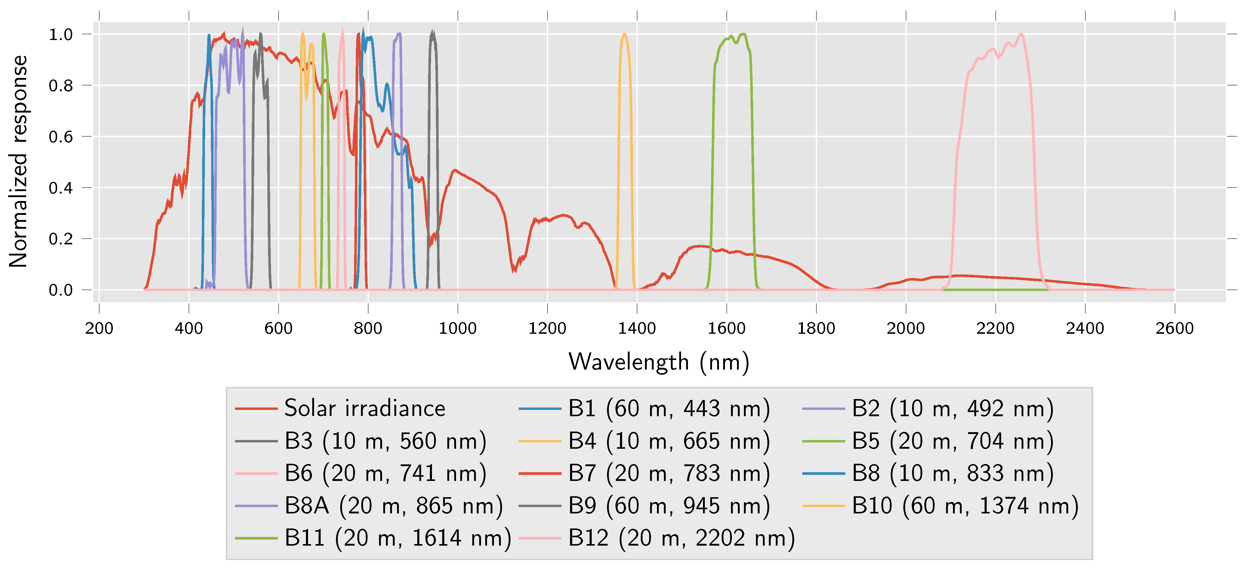
The European Space Agency’s Sentinel-2 (S2) satellite constellation comprises two satellites that carry arrays of multispectral sensors that cover 13 bands in the visible, near-infrared, and shortwave-infrared part of the spectrum. Spectral characteristics of Sentinel-2 A and B sensors can be assumed to be roughly identical for practical purposes and cover the same wavelengths and resolutions [1]. Four bands have 10 spatial resolution, bands , , and in the visible spectrum and in the near-infrared spectrum. Bands , , and have 60 resolution. The remaining bands, , , , , , and , have 20 resolution. As Figure 1 illustrates, bands , , and cover low transmittance wavelengths which makes them harder to process. , the cirrus band, is a water absorption band and is usually ignored outside of cloud cover detection applications, as it does not contain surface information.
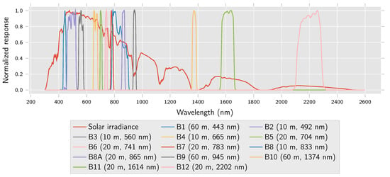
Figure 1.
Sentinel-2 spectral response characteristics from [1] alongside earth surface solar irradiance from [3]. Spatial resolution and central spectral wavelength of each band appear in parentheses in the legend.
Some multispectral satellites, for instance, Landsat-7, capture a high-resolution panchromatic band alongside lower resolution bands of varying spectra which can be used for pansharpening, i.e., transferring detail from the high resolution panchromatic band to the lower resolution bands. S2 does not have high-resolution panchromatic sensors, so pansharpening methods can not be directly applied to S2 data. It is necessary to use S2’s other high-resolution bands when generating super-resolution versions of low-resolution bands, which complicates the process somewhat. Popular pansharpening methods have still been applied to S2 data by selecting or generating high resolution bands, for example, in [2].
Methods have also been developed specifically for super-resolution of S2 images, and considerable prior work is available on the subject. Model based methods explicitly define a model of image degradation to be reversed based on prior knowledge of the image acquisition system, while machine learning based methods learn it directly from the data.
Numerous methods are based on a variational framework which is based on projections onto a subspace justified by a linear sensor model: Super-resolution for multispectral multiresolution estimation (SupReME) [4], Sentinel-2 Sharpening (S2Sharp) [5], Multiresolution Sharpening Approach (MuSA) [6], and Sentinel-2 Super-resolution via Scene-adapted Self-similarity (SSSS) [7].
Area-To-Point Regression Kriging (ATPRK) [8] and Sen2res [9] use somewhat different approaches. ATPRK combines regression and area-to-point kriging to predict higher resolution representations of the low-resolution bands. The point spread function (PSF) of the sensor, size of pixels, and spatial correlation are used for predictions based on the high-resolution bands [8]. The Sen2res method explicitly encodes geometric details from available high-resolution bands as pixel properties independent from their reflectance. It attempts to preserve the spectral content of each low-resolution band independently from the geometry and combine the two to solve the super-resolution problem [9].
A number of deep learning based methods have been proposed for S2 super-resolution. These include Deep Sentinel-2 (DSen2) [10] which was trained at reduced resolution on a random selection of 60 large scenes (∼110 × 110 ). A Deep Residual Network that fuses the fine and coarse spatial resolution bands is suggested in [11]. Sentinel-2 Symmetric Skip Connection convolutional neural network (S2 SSC) [12] extends on this but uses an unsupervised single image learning (zero-shot) approach in which the training and testing are performed on the same image. The only training input is the image for which a super-resolved version is desired. The Remote Sensing Very Deep Super-Resolution [13] (RS-VDSR) network retrains previously developed deep convolutional networks from [14,15] to work with S2 data with promising results. Sentinel-2 Parallel Residual Network [16] (SPRNet) trains two sets of parallel residual networks with lower scale data synthesized from the S2 data, obtaining good spatial fidelity and spectral preservation. The paper [17] was inspired by DSen2 and develops two large neural networks for deployment and training on high performance computing clusters, one for 20 bands and one for 60 bands. Furthermore, inspired by DSen2, ref. [18] suggests a single convolutional neural network for super-resolving the 20 and 60 Sentinel-2 bands to 10 simultaneously.
Variants of Generative Adversarial Networks [19] (GAN) have also been suggested for S2 sharpening. A deep convolutional design for a GAN that gives good results for the super-resolution of S2 images was developed in [20]. Sentinel-2 Generative Adversarial Network [21] (S2GAN) similarly uses the 10 S2 bands as guidance for learning the super-resolution task on lower resolution bands. A GAN method inspired by [22] that focuses solely on the S2 10 RGB bands was developed in [23]. It is trained using PeruSat-1 images with 2.8 m resolution as a reference to resolve S2 images.
When comparing different methods, finding the best parameters for each method can be a daunting task, particularly if a method has many parameters or if the user is not intimately familiar with all the nuances of the method. We present a framework that allows for fair comparisons between different methods by attempting to ensure optimal performance is achieved by each method. Having a framework that can be applied across different methods of super-resolution, or even different capture platforms makes an objective comparison of methods easier.
In this paper, we propose a tuning parameter selection method using Wald’s protocol [24] by first reducing the scale of the image being processed and . Bayesian optimization [25] with a Tree-structured Parzen Estimator [26,27] (TPE) is used to find the parameters that give the best results when resolving the 20 and 60 m bands back to their original resolution and applied to super-resolving the original full scale image. A preliminary version of this parameter selection approach was described in [28]. Our code is available on the first author’s github page (https://github.com/SveinnEirikur/s2-sr-parameter-optimization, accessed on 3 June 2021).
The proposed parameter selection approach is used to select tuning parameters for six S2 sharpening methods, i.e., SupReME, S2Sharp, MuSA, SSSS, ATPRK and S2 SSC. These methods along with DSen2, and Sen2res are critically compared using standard comparison criteria. The code used to generate these comparisons will be made available for download. Adding new methods through simple wrapper functions is easy and allows for both parameter optimization and direct comparisons between methods. While the focus in this paper is on Sentinel-2 images these same principles could also be applied to other types of multispectral multiresolution satellite data, e.g., MODIS, ASTER, Landsat-7, and Landsat-8 [29,30,31].
The paper is organized as follows. Section 2 describes the tuning parameter selection approach and the comparison methods. Section 3 compares the qualities of the methods and describes the quantitative metrics used to compare them. Quantitative comparisons use synthesized and reduced scale S2 data. For qualitative comparisons, real S2 images are used. This is followed by the final conclusions in Section 4.
Notation
In this paper, , , and will be used to refer to the set of images captured by the S2 constellation at each resolution, respectively, is the scene as captured by bands , , , and at 10 resolution, is the scene as captured by bands , , , , , and at 20 resolution and is the scene as captured by bands and at 60 resolution. To indicate that a collection of bands has been resampled, either downsampled, upsampled or super-resolved, the new resolution is added as a superscript, i.e., would mean at 20 resolution and would mean super-resolved to 10 . The capital letter is used in the same way to indicate downsampling in a more general manner.
2. Methods
2.1. Model Based Methods
2.1.1. ATPRK
Area-To-Point Regression Kriging (ATPRK) is a geostatistical approach to super-resolution that was first suggested for use with MODIS data in [32]. It was applied to pansharpening of WorldView-2 and Landsat data in [33] and adapted for S2 images in [8]. ATPRK uses regression-based overall trend estimation and area-to-point-based residual upsampling. Here, trend is the geostatistical term for the spatially varying mean of a spatial process, and residual refers to the variation remaining after removal of the trend. ATPRK accounts explicitly for size of support (pixel), spatial correlation, and Point Spread Function (PSF) of the sensor [8]. While the original code only performed m super-resolution, extending it to perform m super-resolving in exactly the same way is fairly simple.
ATPRK consists of two parts: regression and area-to-point kriging (ATPK). The final ATPRK estimate , is given by
where is the regression prediction and is the ATPK prediction.
2.1.2. Sen2res
Sen2res [9] models the mix of elements within a pixel (e.g., 20% road and 80% vegetation) as a physical property of that pixel, exploiting the geometric consistency of subpixel elements across the MS bands in a similar manner to hyperspectral unmixing [34]. The reflectance of each element is modelled as dependent on the spectral band at which it is observed, relying on local consistency between neighbouring pixels. High resolution bands are used to separate band-independent information from band-dependent reflectance, and the geometric information is used to unmix low-resolution pixels while preserving their overall reflectance [9].
Shared values, , span over multiple pixels and represent the band dependent spectral reflectance of elements that are common to the spanned pixels. They are initialized as the average of the high-resolution pixels that partially cover them. Weights, , are internal to each pixel and represent the proportion of elements within the pixel and are initialized as , where r is the scale difference between the coarse and fine bands. Weights are independent of the spectral band, but is not. The mixing equation for shared values and weights is given as
The weights are non-negative and sum-to-one. and are estimated using an iterative method. The shared values are processed through various normalizations, and geometric means to produce a set of corrected shared values for each coarse band as detailed in [9] and they are then combined with the band independent weights, , to produce high-resolution estimates using (2). The general procedure for the bands is similar.
2.1.3. SupReME
The SupReME (SUPer-REsolution for multispectral Multiresolution Estimation) method proposed in [4] relies strongly on the observation model of the imaging process that generates the low-resolution images (blurring and downsampling). It exploits the fact that spectral bands are correlated and can be represented in a lower-dimensional subspace, learned from the input data. The textural information from the high-resolution bands is utilized by encoding the discontinuities of the data and propagating the spatial information to the lower resolution bands.
The vectorized sharpened image at band i has a low-rank representation , where is and . The sharpened image is estimated by minimizing
Here is the vectorized observed image at band i, is a downsampling operator, and is blurring. The regularization term is a weighted roughness penalty given by
is a diagonal spatial weighting matrix and and are finite difference matrices that approximate vertical and horizontal derivatives of the images in the subspace, respectively [5].
An important part of the method is the estimation of . It is estimated using , where is a blurring matrix representing a 2D cyclic convolution. As , the super-resolved image, is not known, is approximated by upsampling all the bands of to the same high-resolution using bicubic interpolation and blurring each band such that the blur of all the bands is equivalent to the strongest blur of the PSF. Singular value decomposition of this approximation of yields .
SupReME fixes since the first few dimensions are expected to be less affected by noise. Per pixel weights, , are for quadratic smoothing as a spatial regulariser. They are calculated from the Prewitt image gradient magnitude [35] and set to a value between and 1. The minimization is then solved using the Constrained Split Augmented Lagrangian Shrinkage Algorithm (C-SALSA) [36,37,38] and the augmented Lagrangian as detailed in [4].
2.1.4. S2Sharp
S2Sharp [5] is closely related to SupReME. It uses a cyclic descent method that employs conjugate gradients and trust-region optimization to find the reduced-rank approximation and subspace and . The cost function minimized is
This is essentially the same as SupReME apart from each dimension of the p-dimensional subspace having an independent regularization coefficient, , and S2Sharp optimizing as well. This is a non-convex optimization problem and is solved using an iterative algorithm. is initialized using the same method as SupReME and refined during cyclic descent. Then cyclic descent is performed using the linear conjugate gradient method and a trust-region method as described in [5].
2.1.5. MuSA
MuSA [6] is also related to SupReME and S2Sharp. SALSA is used to solve the same dimensionally reduced formulation of the problem
The subspace is estimated in an identical manner as in SupReME with the number of dimensions fixed at . Here, regularization is performed with the Color Block Matching 3D Denoiser (C-BM3D) [39], used as a plug-and-play patch-based regularizer [40]. C-BM3D is a variant of the block matching 3D denoiser developed in [41,42] meant for color images. It is used in place of a proximity operator of the kind described in [43,44]. The optimization is based on the SALSA algorithm as detailed in [6].
2.1.6. SSSS
Sentinel-2 Super-resolution via Scene-adapted Self-similarity (SSSS) [7], belongs to the same family of methods as SupReME, S2Sharp, and MuSA. It uses the same dimensionality reduction, but reformulates the regularization term as
where serves as an operator that shifts the kth patch of size from an n-pixel image and is the self-similarity graph collecting pairs of indexes of similar patches. The self-similarity measure is generated using
from a reference image generated by averaging the 10 bands. is learned by adding the most similar yet distinct patch l for each patch k to the graph. The optimization is a variant of the SALSA algorithm and is detailed in [7].
2.2. Deep-Learning Based Methods
2.2.1. DSen2
The DSen2 network was developed in [10] is a fully convolutional neural network, with ResNet inspired skip connections, and can handle images of arbitrary size. Two forms of the network were trained on and pixel patches, respectively, for and super-resolution. Inputs are upsampled to the target resolution using simple bi-linear interpolation before they are fed into the network. The first network is trained using the 10 and 20 bands, while the second network is trained using all bands. They are otherwise the same. The network loss function is the mean absolute error between the network output and the training target. Training is performed using Wald’s protocol. Image bands are downsampled, m and m to train the m network and m, m, and m to train the m network.
Bilinear interpolation is used, so all bands have the same pixel counts before inputting them as training data. The m network is trained with as the target and and as the input. The m network with as the target and , and as the input. Scale-invariance is assumed to assure the network’s usefulness for the actual m and m task.
The network has been trained on 60 varied scenes from across the globe. Actual S2 data tiles were gathered from the Copernicus Services Data Hub, picked randomly, aiming for a roughly even distribution over the globe and for variety in terms of climate zone, land-cover, and biome type. In regard to the generation of training data [10] directly references the applicability of the S2 PSF, but in practice, the code supplied by the authors does not utilize it. Instead training data is generated by simply filtering the bands with a Gaussian filter with and an boxcar filter followed by downsampling by s, where s is either 2 or 6.
2.2.2. S2 SSC
The S2 SSC [12] convolutional neural network is inspired by the U-net architecture [45] and the networks in [11,46]. It uses a single image learning approach that allows training and testing using the same image. Unlike the other methods studied in this paper, this network only super-resolves the 20 bands of the S2 data, not the 60 bands. The network is trained by using small overlapping training patches with a spatial size of and a stride of 8 on the spatial axes. The loss function is given by the mean squared error between the network output and the training target.
Training is performed using Wald’s protocol, the image bands are downsampled, m and m. Two different downsampling methods for training data are tested. In [12], the network used a bilinear interpolation downsampling method to generate the and training data, similar to DSen2. The tuned method uses each bands PSF to generate the reduced scale training images.
As in the previous network, interpolation is used to ensure all bands are at the desired pixel resolution before inputting them as training data. The network is trained with patches from as the target and and as the input. The final result is then produced by passing the original full resolution versions of the and bands as input through the trained network, resulting in it outputting at the full 10 resolution.
2.3. Performance Evaluation
Where ground truth is available, we use the root-mean-squared error (RMSE), relative dimensionless global error (ERGAS), universal image quality index (UIQI), spectral angle mapper (SAM) in degrees, signal-to-reconstruction error (SRE) in dB, and structural similarity index measure (SSIM) metrics as illustrated in [24,47,48]. They are used for quantitatively comparing the methods described in Section 2.1 and Section 2.2. In order to give a fair comparison, a set number of edge pixels are left out of metric calculations. The number of pixels to ignore was chosen as six, as suggested for the SSSS method [7].
RMSE measures the size of the error between the estimated image and the ground truth. Lower values are better. It is calculated for the 20 and 60 bands, separately, as well as for the whole scene when ground truth data is available. RMSE is not useful when comparing across different datasets, while the ERGAS and UIQI metrics were developed for that purpose. ERGAS was specifically designed to compare how effectively an image has been super-resolved. It not only normalizes the values with relation to the dynamic range but also with regard to the scale difference between the low initial resolution and high final resolution. ERGAS is therefore calculated separately for the 20 and 60 bands. Lower values are better for ERGAS as well, and an ERGAS below 3 is considered good [24]. SAM maps the angular differences in the spectral signatures of each pixel and returns a value in degrees. A value of zero implies that the spectra are identical, apart from possibly a scaling factor applied identically to all bands. The mean SAM value is calculated over all the pixels in the scene. When ground truth is available, it is calculated for all bands as well as for only the 20 bands.
UIQI takes a value between and 1, with 1 signifying identical images. It measures correlation, luminance distortion, and contrast distortion. SSIM compares local patterns of pixel intensities. It includes normalization factors for the dynamic range of the image. Its values are also in the range with 1 signifying very similar images. SRE measures the ratio between the ground truth pixel values and the estimation error and is reported in . Therefore, somewhat counter-intuitively, for a metric with error in its name, a higher value is better for SRE. UIQI, SSIM, and SRE are calculated independently for each band, and averages are reported for 20 , 60 , and all bands as applicable.
In short, for RMSE, ERGAS, and SAM values closer to 0 are better, while for UIQI and SSIM values closer to 1 are better.
All experiments were run on an AMD Ryzen 9 3900X 12-Core Processor with 16 GB of 2133 MHz DDR4 system memory and GeForce RTX 2070 SUPER graphics processing unit with 8 GB of VRAM. Running times are the average of 10 runs of the same data on this computer.
2.4. Tuning Parameter Selection
Since ground truth data is not available for real-world applications of S2 super-resolution, tuning parameter selection is performed using Wald’s protocol [24]. The process is outlined in the flow graph in Figure 2. Two reduced resolution images are generated, with all bands at both and original pixel size for each image, respectively. Parameters are selected with Hyperopt and used for super-resolution of the full scale data to get the final image. For small images, padding the data may be necessary so that all methods can process the reduced results during the tuning parameter search. Padding is performed using reflective boundary conditions.

Figure 2.
Flow graph showing the parameter tuning process. Scale reduced data is super-resolved back to its original resolution and evaluted against the unscaled data for parameter selection. The parameters are then used to super-resolve the unscaled data to 10 m resolution.
Appropriate filters are applied to their respective bands to simulate the PSF before downsampling by a factor of 2 and 6, respectively, resulting in and pixel scales. S2 sensor data from [49] is used to estimate the variance of the PSF of each S2 band based on the measured modulation transfer function (MTF) values for each band. The standard deviation is calculated as where s is the scale difference.
Tuning parameters are selected with Bayesian optimization (BO) using the TPE algorithm of the Hyperopt Python package [25,26,27]. The parameters that result in the highest average SRE are found using 150 iterations of optimization. During each iteration, the method being tuned is run twice with the parameters suggested by the TPE algorithm, super-resolving the appropriate bands of both reduced images back to the resolution of the original data, and . SRE is calculated between the original data and and and the average SRE is used as a loss for the optimization process. The tuning parameters that give the highest SRE, selected in this manner, at a reduced scale, can then be applied to super-resolve the original data to 10 m resolution. This parameter tuning method has previously been shown to improve the results obtained using S2Sharp [28].
BO attempts to build a probabilistic surrogate model from previous evaluations that allows it to predict which parameters might be ideal. It works best for search spaces with moderate dimensions [50]. For a specific function and a given set of parameters, BO treats the objective function as a black box and attempts to find the parameters that minimize (or maximize) the output. The aim is to find a good set of parameters as quickly as possible [25].
Tunable parameters and the objective or loss function can be defined to suit dissimilar tasks. For super-resolution using a quantitative image quality metric is appropriate. Tuning the parameters of a method for individual images can, in some cases, improve results dramatically. Different tuning parameters may also be needed for different image subjects. Remote sensing images can differ greatly depending on the subject, e.g., whether the area being captured is urban or rural, mountainous or oceanic, tropical or arctic, etc.
The TPE, or Tree-structured Parzen Estimator algorithm, is a hyperparameter optimization algorithm suggested in [26]. Standard BO using Gaussian Processes models the conditional probability distribution , the probability of output y given input x, directly. TPE models , the probabilty of input x given output y and , the probabilty distribution of y. It fits one Gaussian Mixture Model (GMM), , to the set of hyperparameter values with the best loss function values, and another GMM, , to the remaining hyperparameter values. The TPE algorithm maintains sorted lists of observed variables and chooses the hyperparameter value x that maximizes the ratio [27].
The different methods being tested have different tuning parameters. ATPRK has 6 tuning parameters, , , , , , and . These parameters define a search space internal to the method used to select semivariogram functions for kriging. SupReME has a single tuning parameter, the regularization strength . For S2Sharp, p, the number of dimensions of the subspace , can be tuned, as well as the regularization strength for each of the subspace dimensions, . MuSA and SSSS both have regularization tuning parameters, and , due to using similar implementations of SALSA. For S2 SSC, learning rate and batch size and scale reduction are tuned.
Parameter tuning was not performed for DSen2 and Sen2res. DSen2 is provided as a pre-trained neural network and can not be effectively tuned without extensive retraining. Sen2res does expose some tuning parameters, but they do not lend themselves well to optimization and offer minimal improvement possibilities without prohibitive growth in running times.
3. Results
3.1. Real Data Experiments
3.1.1. Qualitative Comparisons Using Real S2 Data
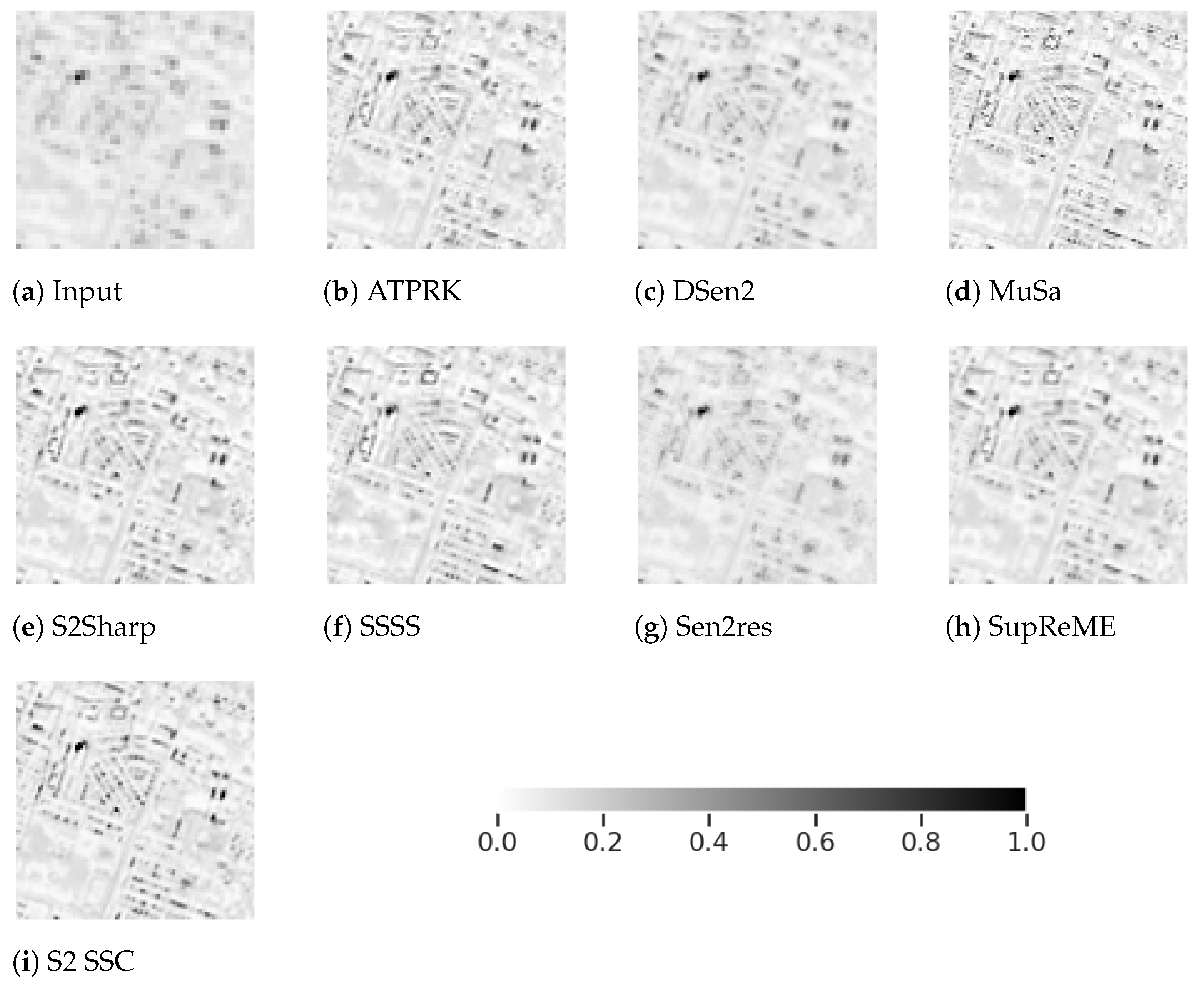
An unprocessed pixel crop from real S2 data seen in Figure 3, showing parts of central Reykjavik in Iceland, was super-resolved using the methods and parameter tuning previously described. The image is part of an S2 tile from the Copernicus Open Access Hub that is 10,000 × 10,000 pixels in the 10 bands captured by Sentinel-2B on a descending orbit at 13:03 on the 17th of October 2019, with Level-2A atmospheric corrections applied [51]. It was chosen for the favorable cloud conditions and presents a very clear view of the capital of Iceland and the surrounding area. Results for each method can be seen in Figure 4 and Figure 5, as pixel crops from bands and , as seen in Figure 3. Very few outliers in the images, having intensity values over 10,000, the expected maximum value, have been clipped and the images normalized by dividing every value by 10,000. These bands are highlighted here because they are particularly hard to super-resolve. No ground truth is available, so quantitative image quality metrics can not be used, and the qualitative comparison is strictly visual.
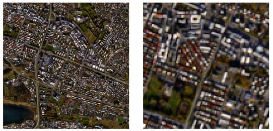
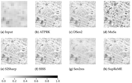
Figure 4.
Band B9 of real S2 image of Reykjavik super-resolved to 10 m resolution.

Figure 5.
Band B12 of real S2 image of Reykjavik super-resolved to 10 m resolution.
For the 60 in Figure 4, ATPRK, S2Sharp, and SSSS appear to give comparatively good results. Rooftop outlines and street layouts are easily discernable and the image contrast looks natural. SupReME, DSen2 and Sen2res, are each successively blurrier and Sen2res returns much lower reflectance values than all the other methods resulting in much lower contrast. MuSA appears oversharpened with overbright outlier pixels. The methods all give fairly similar results for most of the 20 bands but struggle with band in particular. Building shapes are harder to discern and appear irregular compared to the other bands, as seen in Figure 5. Sen2res and DSen2, remain slightly blurry compared to the other methods. S2Sharp, SSSS, SupReME, and S2 SSC appear most natural and visually pleasing. MuSA again appears oversharpened. Making further qualitative judgements is hard due to how similar the results appear.
3.1.2. Quantitative Comparisons Using Reduced Scale S2 Data
To make a quantitative comparison of semi-real S2 data, two reduced scale versions of the same S2 image were generated. First a crop from the data was chosen and reduced resolution versions of all bands were generated at both pixel size and pixel size. This was done by applying appropriate filters to simulate the PSF of each S2 band to their appropriate bands before downgrading by a factor of 2 and 6, respectively.
The blurring being applied is nearly identical to that modelled in the ATPRK, SupReME, S2Sharp, MuSA, and SSSS methods. These data are also scaled to the same scales as the data used for the training process of the DSen2 neural network, while S2 SSC will downgrade the data even further for training. If scale invariance holds, this should not affect the results greatly, but the model based methods and DSen2 may still have a slight advantage. A further crop to pixels for , in , and in was then made for each version of the image, mainly to shorten the running times.
The results can be seen in Table 1 and Table 2, the best results on each line are bold. Although the reduction methods used are the same as for the synthetic data in the following subsection, the errors are much larger for semi-real data. One obvious difference is that here all bands are processed to even lower resolution scales. The scale reduction of the 10 m bands may also be adversely affecting the upscaling processes. The characteristics of real S2 data appear to be worse represented at reduced scales than by synthesized data like that used in the following subsection.

Table 1.
Evaluation using reduced scale S2 data: Reduced by 2, super-resolved m. The best results are given in bold typeface.

Table 2.
Evaluation using reduced scale S2 data: Reduced by 6, super-resolved m. The best results are given in bold typeface.
Based on average RMSE for the m task, the methods ordered by performance are S2 SSC, S2Sharp, ATPRK, SupReME, MuSA, DSen2, Sen2res, and SSSS, as seen in Table 1. SSSS performs significantly worse than its relatives, S2Sharp, SupReME, and MuSA. All methods give fairly good UIQI and SSIM results. For both metrics, the best performances are in bands B6, B7 and B8A. The wavelengths captured in bands B7 and B8A are a subset of the wavelengths captured by the 10 band B8, as can be seen in Figure 1, and B6 is spectrally close. For SRE, the metric being optimized during parameter tuning, ATPRK, S2 SSC, and S2Sharp outperform all other methods by some margin in every 20 band. None of the methods manage to get an ERGAS below 3 for this task, which would be considered a good score.
Table 2 shows that the results are quite different for the m task. MuSA and SSSS perform comparatively well, SSSS giving the best results, followed by MuSA, DSen2, SupReME, S2Sharp, ATPRK, and Sen2res. ATPRK does not perform as well for this data at a greatly reduced scale as for other data tested and in fact the magnitude of the RMSE is greatly increased at this scale for all methods apart from SSSS. ERGAS scores are also fairly high (lower is better) and SRE scores are low (higher is better) for all methods. UIQI and SSIM are also much worse than with the smaller scale reduction, particularly for DSen2 and Sen2res.
3.2. Synthesized Data Experiments
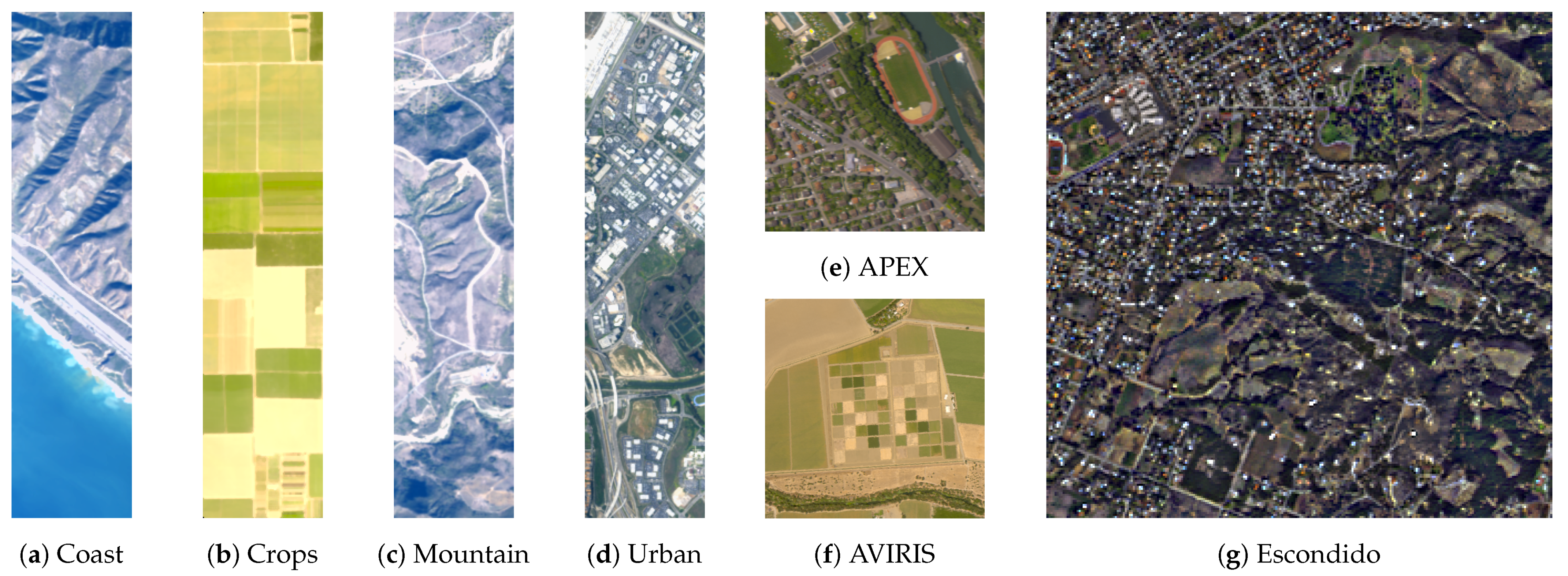
Using the synthetic datasets in Figure 6, quantitative comparisons can be performed. The images shown here as RGB color photos generated from the appropriate spectral bands, are all generated from hyperspectral images. Images a through f, which originate from [4,5,6,7], and the processes used to synthezise them are described in Appendix A. They present varied scenes with coastal, agricultural, rural, urban, and mixed geographies. Section 3.2.2 evalutes the methods using all of the datasets in Figure 6. Section 3.2.1 focuses on Figure 6g, which was generated from AVIRIS [54] data for this paper.
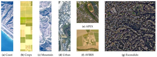
Figure 6.
RGB images of the synthetic datsets used, generated from bands B2, B3 and B4 using a combination of methods described in [52,53].
3.2.1. Quantitative Comparisons Using Synthesized S2 Data
The data for this experiment, seen in Figure 6g, were simulated using an AVIRIS image with 5 resolution employing methods similar to [5,6]. The original AVIRIS image of an area near San Diego, CA, was acquired in November 2011. It is pixels with 5 resolution in 224 bands that span a spectral range of 366–2496 nm that covers the range of the S2 sensors.
The S2 version was simulated by applying the S2 spectral response to a patch of the AVIRIS data depicting parts of the city of Escondido and its suburbs. Twelve bands of size pixels at a spatial resolution of 5 were obtained. These bands were filtered and subsampled and cropped to yield pixel ground truth for all bands at 10 resolution. The bands were then filtered using a Gaussian approximation of the S2 sensor PSF from [49], and downgraded to yield four bands of size pixels at 10 resolution, six bands of size pixels at 20 resolution, and two bands of size pixels at 60 resolution. Because the PSF blur is applied to the synthesized image in a near identical manner to that modeled by the ATPRK, SupReME, S2Sharp, MuSA, and SSSS methods, those methods should be expected to perform particularly well on this data. The tuned version of S2 SSC also uses the same PSF blur during training. Sen2res and DSen2, on the other hand, do not explicitly model the S2 PSF in the same way, so they could be expected to perform worse.
Table 3 shows a comparison between the super-resolution methods. SupReME gets the best results for the 60 bands while ATPRK does slightly better for the 20 bands. Based on average RMSE for all bands, the methods ordered by performance are S2Sharp, ATPRK, SupReME, SSSS, MuSA, DSen2, and Sen2res. For the 20 bands ATPRK is followed by S2 SSC, slightly outperforming S2Sharp. Otherwise, the order remains mostly the same apart from MuSA and SSSS trading places. For 60 band performance, SupReME is followed by S2Sharp, SSSS, ATPRK, MuSA, Sen2res, and DSen2.

Table 3.
Evaluation using S2 data simulated from AVIRIS image of Escondido. The best results are given in bold typeface.
SSSS shows particularly strong results in the 60 bands, getting the best UIQI, SSIM, and SRE scores for B1. DSen2, in contrast, does very badly in band B1 and has the lowest average 60 SRE of all the methods, while Sen2res does slightly worse in all other metrics. ATPRK, MuSA, S2Sharp, S2 SSC, SSSS, and SupReME all get very high 20 UIQI and SSIM scores, with only bands B11 and B12 presenting a significant challenge. Depending on the application, any of these methods might be useful for the lower wavelength 20 bands but based on the low RMSE and high SRE values, ATPRK, S2 SSC, and S2Sharp have a clear advantage.
As noted, due to the lack of PSF modeling, Sen2res and DSen2 were expected to perform slightly worse than the competing methods.
For all data, running times are dominated by DSen2. It processes this particular data in approximately half a second. The slowest method by far is MuSA, which takes almost 2 5 min to process the same image. The other methods are much quicker, taking about 15 s each, apart from SSSS which takes slightly under 1 min.
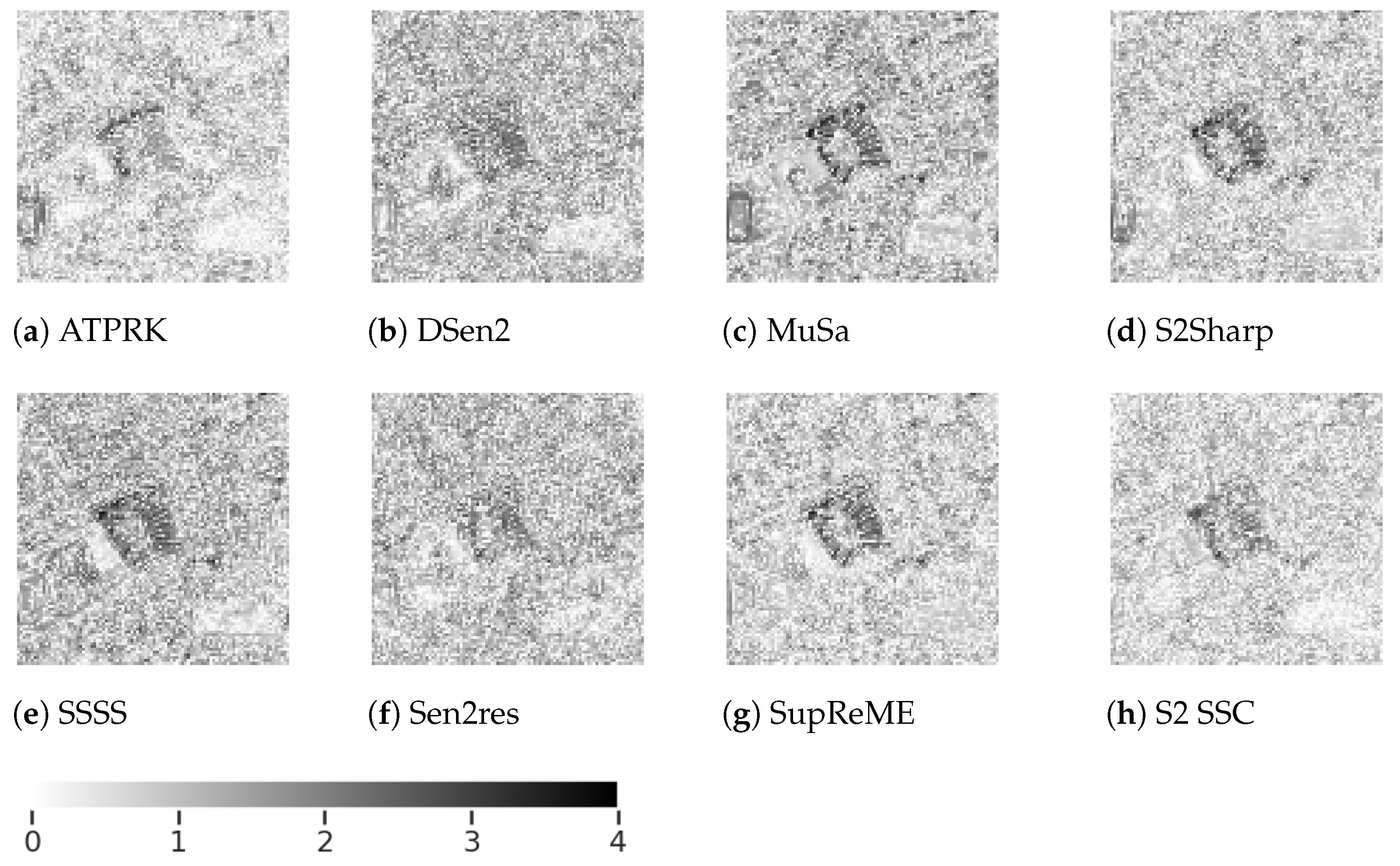
Error maps showing a graphical representation of the error between the estimates of each method and the reference ground truth as logarithmically scaled residual images, calculated using can be seen in Figure 7 and Figure 8. These residual images for bands B9 and B12, respectively, are shown on a scale of 0 to 4. These bands are again highlighted because they are hard to super-resolve.
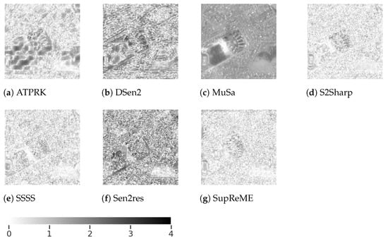
Figure 7.
Absolute error map of Escondido crop, band B9, on log scale. Lower values are better.

Figure 8.
Absolute error map of Escondido crop, band B12, on log scale. Lower values are better.
MuSA appears to have a constant error in the 60 band, B9, as can be seen in Figure 7c but does much better for B12. Strange geometrical patterns are also visible in the 60 → 10 ATPRK image in subfigure a. The disadvantages of DSen2 and Sen2res are visible in subfigures b and f, respectively. Their residuals are larger than for the remaining methods. SSSS appears to give the best results in this case, with the least apparent structural textures visible in subfigure e, despite Table 3 showing that it has higher 60 RMSE than S2Sharp and SupReME, whose localized errors are more eye-catching.
The results for B12 are more similar. The fact that building shapes are discernible in most error maps suggests structural image definition has been lost compared to the ground truths. In Figure 8 the errors appear to be more evenly distributed over the whole image for DSen2 and Sen2res. More localized errors reveal clear building shapes with Musa, S2Sharp, SSSS, and SupReME. ATPRK and S2 SSC give the visibly best result, which broadly matches the SRE results in Table 3.
3.2.2. Evaluating Effects of Parameter Tuning
The parameter tuning method was evaluated for each of the super-resolution methods by testing them on the 7 datasets seen in Figure 6. The 6 additional synthesized S2 datasets were originally used for testing some of the methods in their original papers and their generation is described in greater detail in Appendix A. These images all come with ground truths and were super-resolved using both default and tuned parameters.
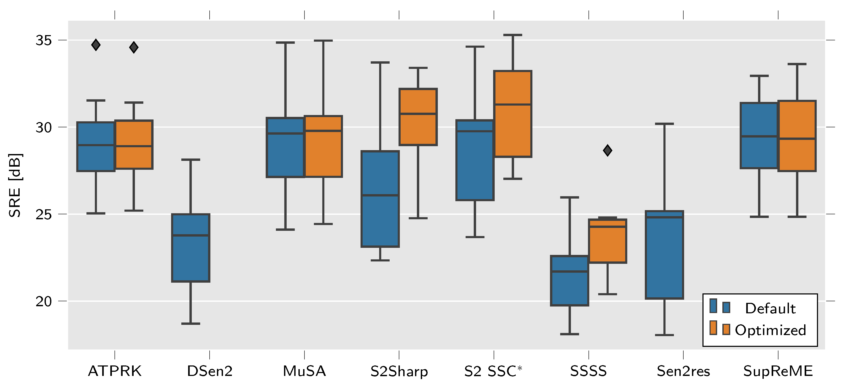
Parameter tuning was performed as previously described and the boxplots of Figure 9 show a comparison of the SRE values for each method. While ATPRK, MuSA and SupReME show almost no improvements, S2Sharp, S2 SSC, and SSSS show significant gains from the use of parameter tuning method.
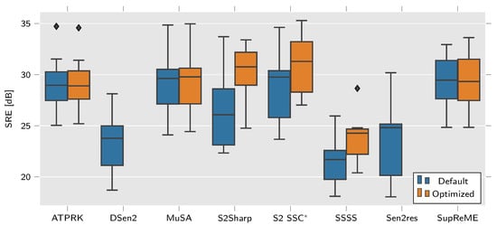
Figure 9.
Boxplot showing the distribution of SRE in dB for all the synthetic datasets for each of the methods. Higher values are better. S2 SSC is only evaluted for 20 m bands but other methods include values for both 20 and 60 m bands.
ATPRK performs a parameter search of its own to select the best values for the semivariograms used to generate the kriging matrix. The parameters being tuned here merely provides initialization for that search which might explain why ATPRK does not show much of an improvement. Parameter tuning does not appreciably improve MuSA performance and tweaking the single parameter of SupReME does not seem to affect the results in any significant manner either. These methods may also have already been tuned to the ideally suited parameters.
Focusing on the mean SRE, represented by a line inside each box on the boxplot, S2Sharp, S2 SSC, and SSSS all benefit greatly from the use of tuned parameters. Unlike the related MuSA method the selection of different and is very effective for SSSS. The end results still remain rather unimpressive compared to the other methods, even with tuning. SSSS appears ill suited for the type of synthetic data being tested.
For a fixed number of iterations, the tuning being performed on the S2 SSC batch size and learning rate is probably affecting how quickly the network finds a solution more than the quality of the solution. The improvement is mainly a result of the change in how training images are generated. Using PSF modeling for the synthesized data increases the methods performance significantly. It should still be reiterated that S2 SSC only processes the 20 bands.
S2Sharp goes from middling, using default parameters, to leading performance when tuned. The performance boost is to be expected as the method was developed with an associated parameter tuning method presented in [5] and not really intended to be used with the default parameters for all data. As was shown in [28] the parameter tuning method used here can further improve its results.
Broadly, Figure 9 shows that with tuning S2Sharp gives the best results, on average, and S2 SSC does best for the 20 bands. Without tuning ATPRK, MuSA, and SupReME can potentially perform better. The other methods, DSen2, Sen2res, and SSSS do not perform as well.
4. Conclusions
It is apparent that three methods, ATPRK, S2Sharp, and S2 SSC, outperform the other methods used in the experiments. ATPRK is easy to use and gives good results without the need for specifically tuning it to the data and may be good enough for many applications. Although improved results can be gained by using S2Sharp with tuned parameters, this requires parameter tuning for each dataset that is to be processed. It is less practical in general use even though on average it outperforms the other methods quantitatively for the data tested. For 20 → 10 super-resolution S2 SSC yields the best performance, highlighting the potential of deep learning methods. The tuning method proposed, while somewhat time-consuming, can be easily applied to all S2 super-resolution methods that benefit from parameter tuning. It was shown to greatly improve the results for S2Sharp and SSSS. The tuning parameters selected for the other methods had little effect on the end results, suggesting their default parameters were already a good fit for the data being tested and that the tuning method can reliably find similarly good parameters using reduced scale data.
Author Contributions
Investigation, data curation and writing—original draft preparation, S.E.A.; writing—review and editing, M.O.U., J.S. and J.R.S.; software, S.E.A., M.O.U. and H.V.N. All authors have read and agreed to the published version of the manuscript.
Funding
This research was funded in part by The Icelandic Research Fund under Grant 207233-051.
Institutional Review Board Statement
Not applicable.
Informed Consent Statement
Not applicable.
Data Availability Statement
Publicly available datasets were analyzed in this study. This data can be found here: https://aviris.jpl.nasa.gov/, https://scihub.copernicus.eu/, https://github.com/lanha/SupReME.
Acknowledgments
We would like to thank the authors of Sen2res, Nicolas Brodu (GEOSTAT team at Inria), and of SupReME and DSen2, Charis Lanaras (ETH Zürich), for making their code publicly available, as well as Chia-Hsiang Lin (National Cheng Kung University), author of SSSS, Claudia Paris (University of Trento), author of MuSA, and Qunming Wang (Tongji University), author of ATPRK, for providing code and data upon request.
Conflicts of Interest
The authors declare no conflict of interest.
Abbreviations
| ATPRK | Area-To-Point Regression Kriging |
| C-BM3D | Color Block Matching 3D Denoiser |
| DSen2 | Deep Sentinel-2 |
| ERGAS | relative dimensionless global error |
| GAN | Generative Adversarial Networks |
| GMM | Gaussian Mixture Model |
| MS | Multi-Spectral |
| MTF | Modulation Transfer Function |
| MuSA | Multiresolution Sharpening Approach |
| PSF | Point Spread Function |
| RMSE | Root-Mean-Squared Error |
| S2 | Sentinel-2 |
| S2 SSC | Sentinel-2 Symmetric Skip Connection |
| S2Sharp | Sentinel-2 Sharpening |
| SALSA | Split Augmented Lagrangian Shrinkage Algorithm |
| SAM | Spectral Angle Mapper |
| SRE | Signal-to-Reconstruction Error |
| SRF | Spectral Response Functions |
| SSIM | Structural Similarity Index Measure |
| SSSS | Sentinel-2 Super-resolution via Scene-adapted Self-similarity |
| SupReME | Super-resolution for multispectral multiresolution estimation |
| TPE | Tree-structured Parzen Estimator |
| UIQI | Universal Image Quality Index |
Appendix A. Descriptions of Datasets
Descriptions of datasets used in Section 3.2.2 follow. Example data was provided with some of the published code for the methods in Section 2, and some authors were kind enough to share test data upon request.
Appendix A.1. S2Sharp
This dataset is simulated using an AVIRIS image of an area just outside Sacramento, CA, that was acquired in August 2013. The image is pixels in 197 usable bands that span a similar spectral range as the S2 sensor. The S2 version was simulated by applying the S2 spectral response to the AVIRIS data. Twelve bands of size pixels at a spatial resolution of m were obtained.
Appropriate bands were filtered using an estimated point spread function of the S2 sensor and downgraded to yield four bands of size pixels at m resolution, six bands of size pixels at m resolution, and two bands of size pixels at m resolution. Zero-mean identically and independently distributed (i.i.d.) Gaussian noise is added for 40 dB SNR [5]. The scale ratio between bands is therefore the same, although the actual pixel sizes differ from S2’s 10 m, 20 m and 60 m.
Appendix A.2. SupReME
The SupReME method includes a sample S2 dataset simulated from part of the Open Science APEX dataset [55,56]. The method to generate this dataset is nearly identical to that used in the S2Sharp paper. The spatial reolution of this image is pixels at 2 m resolution for , pixels at 4 m resolution for and pixels at 12 m resolution for . I.i.d. Gaussian noise is also added for 40 dB SNR [4].
Appendix A.3. MuSA and SSSS
The MuSA and SSSS methods both use the same four AVIRIS images of differing scenes showing coastal, mountainous, urban and agricultural geography. Ground-truth images were generated by low-pass filtering and subsampling the 5 coastal and mountain data by 2 and the, respectively, m and m urban and crop datasets by 3.
After low-pass filtering, the S2 spectral responses were applied, followed by the S2 sensor PSF’s and further subsampling of and so that all bands have approximately the same pixel sizes as actual S2 data. Finally i.i.d. zero-mean Gaussian noise is added for 40 dB SNR [6].
References
- European Space Agency. Sentinel-2 Spectral Response Functions (S2-SRF). Sentinel-2 MSI Document Library. 2017. Available online: https://sentinel.esa.int/web/sentinel/user-guides/sentinel-2-msi/document-library (accessed on 2 June 2021).
- Kaplan, G. Sentinel-2 Pan Sharpening—Comparative Analysis. Proceedings 2018, 2, 345. [Google Scholar] [CrossRef]
- G03 Committee. Tables for Reference Solar Spectral Irradiances: Direct Normal and Hemispherical on 37 Tilted Surface; Technical Report; ASTM International: West Conshohocken, PA, USA, 2012. [Google Scholar] [CrossRef]
- Lanaras, C.; Bioucas-Dias, J.M.; Baltsavias, E.; Schindler, K. Super-Resolution of Multispectral Multiresolution Images from a Single Sensor. In Proceedings of the 2017 IEEE Conference on Computer Vision and Pattern Recognition Workshops (CVPRW), Honolulu, HI, USA, 21–26 July 2017; pp. 1505–1513. [Google Scholar] [CrossRef]
- Ulfarsson, M.O.; Palsson, F.; Mura, M.D.; Sveinsson, J.R. Sentinel-2 Sharpening Using a Reduced-Rank Method. IEEE Trans. Geosci. Remote Sens. 2019, 57, 6408–6420. [Google Scholar] [CrossRef]
- Paris, C.; Bioucas-Dias, J.M.; Bruzzone, L. A Novel Sharpening Approach for Superresolving Multiresolution Optical Images. IEEE Trans. Geosci. Remote Sens. 2019, 57, 1545–1560. [Google Scholar] [CrossRef]
- Lin, C.H.; Bioucas-Dias, J.M. An Explicit and Scene-Adapted Definition of Convex Self-Similarity Prior With Application to Unsupervised Sentinel-2 Super-Resolution. IEEE Trans. Geosci. Remote Sens. 2020, 58, 3352–3365. [Google Scholar] [CrossRef]
- Wang, Q.; Shi, W.; Li, Z.; Atkinson, P.M. Fusion of Sentinel-2 Images. Remote Sens. Environ. 2016, 187, 241–252. [Google Scholar] [CrossRef]
- Brodu, N. Super-Resolving Multiresolution Images With Band-Independent Geometry of Multispectral Pixels. IEEE Trans. Geosci. Remote Sens. 2017, 55, 4610–4617. [Google Scholar] [CrossRef]
- Lanaras, C.; Bioucas-Dias, J.M.; Galliani, S.; Baltsavias, E.; Schindler, K. Super-Resolution of Sentinel-2 Images: Learning a Globally Applicable Deep Neural Network. ISPRS J. Photogramm. Remote Sens. 2018, 146, 305–319. [Google Scholar] [CrossRef]
- Palsson, F.; Sveinsson, J.R.; Ulfarsson, M.O. Sentinel-2 Image Fusion Using a Deep Residual Network. Remote Sens. 2018, 10, 1290. [Google Scholar] [CrossRef]
- Nguyen, H.V.; Ulfarsson, M.O.; Sveinsson, J.R.; Sigurdsson, J. Zero-Shot Sentinel-2 Sharpening Using a Symmetric Skipped Connection Convolutional Neural Network. In Proceedings of the IGARSS 2020—2020 IEEE International Geoscience and Remote Sensing Symposium, Waikoloa, HI, USA, 26 September–2 October 2020; pp. 613–616. [Google Scholar] [CrossRef]
- Panagiotopoulou, A.; Grammatikopoulos, L.; Charou, E.; Bratsolis, E.; Madamopoulos, N.; Petrogonas, J. Very Deep Super-Resolution of Remotely Sensed Images with Mean Square Error and Var-Norm Estimators as Loss Functions. arXiv 2020, arXiv:2007.15417. [Google Scholar]
- Kim, J.; Lee, J.K.; Lee, K.M. Accurate Image Super-Resolution Using Very Deep Convolutional Networks. In Proceedings of the 2016 IEEE Conference on Computer Vision and Pattern Recognition (CVPR), Las Vegas, NV, USA, 27–30 June 2016; pp. 1646–1654. [Google Scholar] [CrossRef]
- Zioga, E.; Panagiotopoulou, A.; Stefouli, M.; Charou, E.; Grammatikopoulos, L.; Bratsolis, E.; Madamopoulos, N. Spatial Resolution Increase of Remotely Sensed Images from Mining Areas with Deep Learning Techniques. arXiv 2020, arXiv:2007.08791. [Google Scholar]
- Wu, J.; He, Z.; Hu, J. Sentinel-2 Sharpening via Parallel Residual Network. Remote Sens. 2020, 12, 279. [Google Scholar] [CrossRef]
- Zhang, R.; Cavallaro, G.; Jitsev, J. Super-Resolution of Large Volumes of Sentinel-2 Images with High Performance Distributed Deep Learning; Technical Report FZJ-2020-04989; Jülich Supercomputing Center: Jülich, Germany, 2020. [Google Scholar]
- Esquena Calm, O. Super-Resolution of Sentinel-2 Images a Single Network for All-Bands Upsampling. Bachelor’s Thesis, Universitat Politècnica de Catalunya, Barcelona, Spain, 2020. [Google Scholar]
- Goodfellow, I.J.; Pouget-Abadie, J.; Mirza, M.; Xu, B.; Warde-Farley, D.; Ozair, S.; Courville, A.; Bengio, Y. Generative Adversarial Nets. In Proceedings of the 27th International Conference on Neural Information Processing Systems, NIPS’14; MIT Press: Cambridge, MA, USA, 2014; Volume 2, pp. 2672–2680. [Google Scholar]
- Palsson, F.; Sveinsson, J.R.; Ulfarsson, M.O. Single Sensor Image Fusion Using A Deep Convolutional Generative Adversarial Network. In Proceedings of the 2018 9th Workshop on Hyperspectral Image and Signal Processing: Evolution in Remote Sensing (WHISPERS), Amsterdam, The Netherlands, 23–26 September 2018; pp. 1–5. [Google Scholar] [CrossRef]
- Zhang, K.; Sumbul, G.; Demir, B. An Approach to Super-Resolution of Sentinel-2 Images Based on Generative Adversarial Networks. arXiv 2020, arXiv:1912.06013. [Google Scholar]
- Ledig, C.; Theis, L.; Huszár, F.; Caballero, J.; Cunningham, A.; Acosta, A.; Aitken, A.; Tejani, A.; Totz, J.; Wang, Z.; et al. Photo-Realistic Single Image Super-Resolution Using a Generative Adversarial Network. In Proceedings of the 2017 IEEE Conference on Computer Vision and Pattern Recognition (CVPR), Honolulu, HI, USA, 21–26 July 2017; pp. 105–114. [Google Scholar] [CrossRef]
- Pineda, F.; Ayma, V.; Beltran, C. A Generative Adversarial Network Approach for Super-Resolution of Sentinel-2 Satellite Images. In The International Archives of Photogrammetry, Remote Sensing and Spatial Information Sciences; Copernicus GmbH: Gottingen, Germany, 2020; Volume XLIII-B1-2020, pp. 9–14. [Google Scholar] [CrossRef]
- Wald, L. Assessing the Quality of Synthesized Images. In Data Fusion. Definitions and Architectures—Fusion of Images of Different Spatial Resolutions; Les Presses de l’École des Mines: Paris, France, 2002. [Google Scholar]
- Snoek, J.; Larochelle, H.; Adams, R.P. Practical Bayesian Optimization of Machine Learning Algorithms. Adv. Neural Inf. Process. Syst. 2012, 25, 2951–2959. [Google Scholar]
- Bergstra, J.; Bardenet, R.; Bengio, Y.; Kégl, B. Algorithms for Hyper-Parameter Optimization. Adv. Neural Inf. Process. Syst. 2011, 24, 2546–2554. [Google Scholar]
- Bergstra, J.; Yamins, D.; Cox, D. Making a Science of Model Search: Hyperparameter Optimization in Hundreds of Dimensions for Vision Architectures. In Proceedings of the 30th International Conference on Machine Learning, Atlanta, GA, USA, 16–21 June 2013; pp. 115–123. [Google Scholar]
- Armannsson, S.E.; Sigurdsson, J.; Sveinsson, J.R.; Ulfarsson, M.O. Tuning Parameter Selection for Sentinel-2 Sharpening Using Wald’s Protocol. In Proceedings of the IEEE International Geoscience Remote Sensing Symposium, Brussels, Belgium, 12–16 July 2021. [Google Scholar]
- Masek, J.G. Landsat 8 Overview|Landsat Science. 2013. Available online: https://landsat.gsfc.nasa.gov/landsat-8/landsat-8-overview (accessed on 2 June 2021).
- Thome, K. ASTER|Terra. 2021. Available online: https://terra.nasa.gov/about/terra-instruments/aster (accessed on 2 June 2021).
- Thome, K. MODIS|Terra. 2021. Available online: https://terra.nasa.gov/about/terra-instruments/modis (accessed on 2 June 2021).
- Wang, Q.; Shi, W.; Atkinson, P.M.; Zhao, Y. Downscaling MODIS Images with Area-to-Point Regression Kriging. Remote Sens. Environ. 2015, 166, 191–204. [Google Scholar] [CrossRef]
- Wang, Q.; Shi, W.; Atkinson, P.M. Area-to-Point Regression Kriging for Pan-Sharpening. ISPRS J. Photogramm. Remote Sens. 2016, 114, 151–165. [Google Scholar] [CrossRef]
- Keshava, N.; Mustard, J. Spectral Unmixing. IEEE Signal Process. Mag. 2002, 19, 44–57. [Google Scholar] [CrossRef]
- Prewitt, J. Object Enhancement and Extraction. In Picture Processing and Psychopictorics; Elsevier Science: Saint Louis, MO, USA, 1970; pp. 75–149. [Google Scholar]
- Afonso, M.V.; Bioucas-Dias, J.M.; Figueiredo, M.A.T. A Fast Algorithm for the Constrained Formulation of Compressive Image Reconstruction and Other Linear Inverse Problems. In Proceedings of the 2010 IEEE International Conference on Acoustics, Speech and Signal Processing, Dallas, TX, USA, 14–19 March 2010; pp. 4034–4037. [Google Scholar] [CrossRef]
- Afonso, M.V.; Bioucas-Dias, J.M.; Figueiredo, M.A.T. Fast Image Recovery Using Variable Splitting and Constrained Optimization. IEEE Trans. Image Process. 2010, 19, 2345–2356. [Google Scholar] [CrossRef]
- Afonso, M.V.; Bioucas-Dias, J.M.; Figueiredo, M.A.T. An Augmented Lagrangian Approach to the Constrained Optimization Formulation of Imaging Inverse Problems. IEEE Trans. Image Process. 2011, 20, 681–695. [Google Scholar] [CrossRef]
- Dabov, K.; Foi, A.; Katkovnik, V.; Egiazarian, K. Color Image Denoising via Sparse 3D Collaborative Filtering with Grouping Constraint in Luminance-Chrominance Space. In Proceedings of the 2007 IEEE International Conference on Image Processing, San Antonio, TX, USA, 16 September–19 October 2007; Volume 1, pp. I-313–I-316. [Google Scholar] [CrossRef]
- Venkatakrishnan, S.V.; Bouman, C.A.; Wohlberg, B. Plug-and-Play Priors for Model Based Reconstruction. In Proceedings of the 2013 IEEE Global Conference on Signal and Information Processing, Austin, TX, USA, 3–5 December 2013; pp. 945–948. [Google Scholar] [CrossRef]
- Dabov, K.; Foi, A.; Katkovnik, V.; Egiazarian, K. Image Denoising with Block-Matching and 3D Filtering. In Image Processing: Algorithms and Systems, Neural Networks, and Machine Learning; International Society for Optics and Photonics: San Jose, CA, USA, 2006; Volume 6064, p. 606414. [Google Scholar] [CrossRef]
- Dabov, K.; Foi, A.; Katkovnik, V.; Egiazarian, K. Image Denoising by Sparse 3-D Transform-Domain Collaborative Filtering. IEEE Trans. Image Process. 2007, 16, 2080–2095. [Google Scholar] [CrossRef]
- Combettes, P.L.; Wajs, V.R. Signal Recovery by Proximal Forward-Backward Splitting. Multiscale Model. Simul. 2005. [Google Scholar] [CrossRef]
- Combettes, P.L.; Pesquet, J.C. Proximal Splitting Methods in Signal Processing. In Fixed-Point Algorithms for Inverse Problems in Science and Engineering; Bauschke, H.H., Burachik, R.S., Combettes, P.L., Elser, V., Luke, D.R., Wolkowicz, H., Eds.; Springer Optimization and Its Applications; Springer: New York, NY, USA, 2011; pp. 185–212. [Google Scholar] [CrossRef]
- Ronneberger, O.; Fischer, P.; Brox, T. U-Net: Convolutional Networks for Biomedical Image Segmentation. In Medical Image Computing and Computer-Assisted Intervention –MICCAI 2015; Navab, N., Hornegger, J., Wells, W.M., Frangi, A.F., Eds.; Springer International Publishing: Cham, Switzerland, 2015; pp. 234–241. [Google Scholar]
- Shocher, A.; Cohen, N.; Irani, M. “Zero-Shot” Super-Resolution Using Deep Internal Learning. arXiv 2017, arXiv:1712.06087. [Google Scholar]
- Wang, Z.; Bovik, A. A Universal Image Quality Index. IEEE Signal Process. Lett. 2002, 9, 81–84. [Google Scholar] [CrossRef]
- Jagalingam, P.; Hegde, A.V. A Review of Quality Metrics for Fused Image. Aquat. Procedia 2015, 4, 133–142. [Google Scholar] [CrossRef]
- Clerc, S.; MPC-Team. S2 MPC—Data Quality Report; Technical Report 05, Online, Reference S2-PDGS-MPC-DQR; European Space Agency: Paris, France, 2016; Available online: https://sentinel.esa.int/documents/247904/685211/Sentinel-2+Data+Quality+Report+(DQR)/ (accessed on 2 June 2021).
- Shahriari, B.; Swersky, K.; Wang, Z.; Adams, R.P.; de Freitas, N. Taking the Human Out of the Loop: A Review of Bayesian Optimization. Proc. IEEE 2016, 104, 148–175. [Google Scholar] [CrossRef]
- European Space Agency. S2B_MSIL2A_20191017T130259_N0213_R038_T27WVM_20191017T134229; Copernicus Open Access Hub. 2021. Available online: https://scihub.copernicus.eu/ (accessed on 2 June 2021).
- Magnusson, M.; Sigurdsson, J.; Armansson, S.E.; Ulfarsson, M.O.; Sveinsson, J.R.; Deborah, H. Creating RGB Images from Hyperspectral Images Using a Color Matching Function. In Proceedings of the IGARSS 2020—2020 IEEE International Geoscience and Remote Sensing Symposium, Waikoloa, HI, USA, 26 September–2 October 2020; pp. 2045–2048. [Google Scholar] [CrossRef]
- Sovdat, B.; Kadunc, M.; Batič, M.; Milčinski, G. Natural Color Representation of Sentinel-2 Data. Remote Sens. Environ. 2019, 225, 392–402. [Google Scholar] [CrossRef]
- NASA Jet Propulsion Laboratory. Flight f111116t01p00r12; AVIRIS Data Portal. 2021. Available online: https://aviris.jpl.nasa.gov/ (accessed on 2 June 2021).
- European Space Agency. APEX; APEX Open Science Data Set. 2021. Available online: https://apex-esa.org/en/data/free-data-cubes (accessed on 2 June 2021).
- Schaepman, M.; Jehle, M.; Hueni, A.; D’Odorico, P.; Damm, A.; Weyermann, J.; Schneider, F.D.; Laurent, V.; Popp, C.; Seidel, F.C.; et al. Advanced radiometry measurements and Earth science applications with the Airborne Prism Experiment (APEX). Remote Sens. Environ. 2015, 158, 207–219. [Google Scholar] [CrossRef]
Publisher’s Note: MDPI stays neutral with regard to jurisdictional claims in published maps and institutional affiliations. |
© 2021 by the authors. Licensee MDPI, Basel, Switzerland. This article is an open access article distributed under the terms and conditions of the Creative Commons Attribution (CC BY) license (https://creativecommons.org/licenses/by/4.0/).

