Abstract
This study aims to design a robust particle filter using artificial intelligence algorithms to enhance estimation performance using a low-grade interferometric radar altimeter (IRA). Based on the synthetic aperture radar (SAR) interferometry technology, the IRA can extract three-dimensional ground coordinates with at least two antennas. However, some IRA uncertainties caused by geometric factors and IRA-inherent measurement errors have proven to be difficult to eliminate by signal processing. These uncertainties contaminate IRA outputs, crucially impacting the navigation performance of low-grade IRA sensors in particular. To deal with such uncertainties, an ant-mutated immune particle filter (AMIPF) is proposed. The proposed filter combines the ant colony optimization (ACO) algorithm with the immune auxiliary particle filter (IAPF) to bring individual mutation intensity. The immune system indicates the stochastic parameters of the ACO, which conducts the mutation process in one step for the purpose of computational efficiency. The ant mutation then moves particles into the most desirable position using parameters from the immune system to obtain optimal particle diversity. To verify the performance of the proposed filter, a terrain referenced navigation (TRN) simulation was conducted on an unmanned aerial vehicle (UAV). The Monte Carlo simulation results show that the proposed filter is not only more computationally efficient than the IAPF but also outperforms both the IAPF and the auxiliary particle filter (APF) in navigation performance and robustness.
1. Introduction
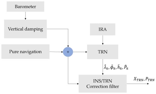
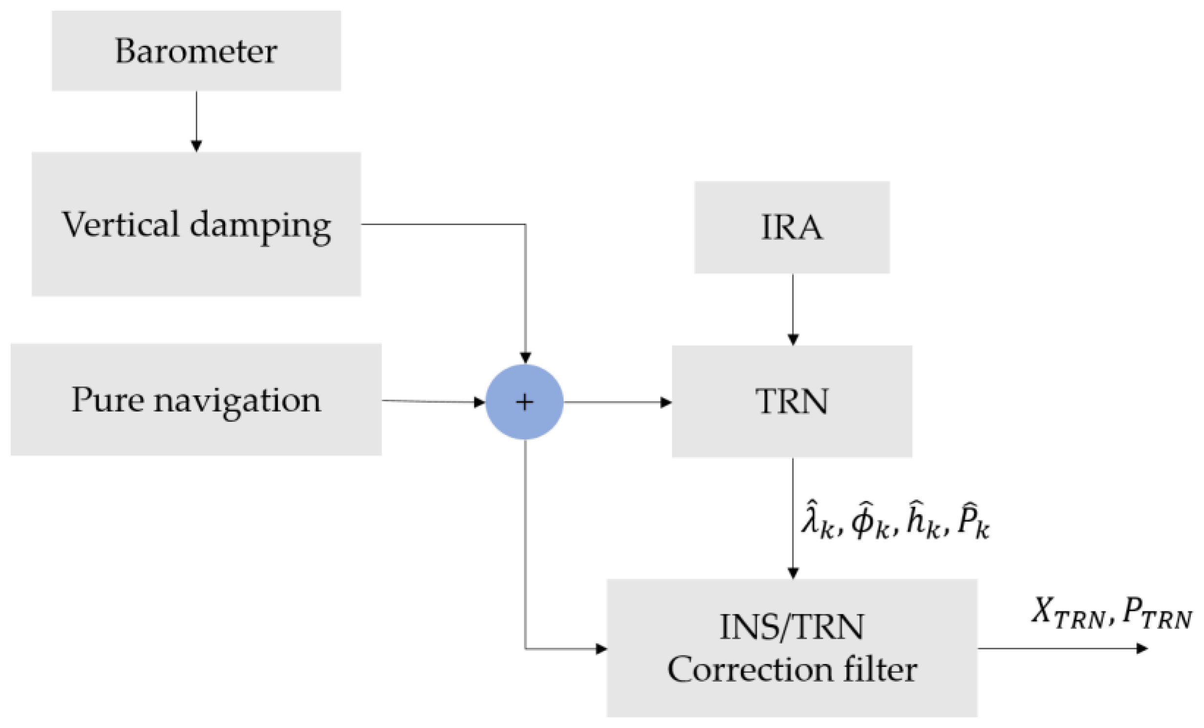
Recently, unmanned aerial vehicles (UAV) have played a vital role in military applications such as reconnaissance and surveillance missions since they allow access to places where conditions are harsh or inhospitable to humans. As indicated by the name, UAVs must possess the autonomous navigation ability to successfully carry out missions. The most popular navigation system for UAVs is a combination of the inertial navigation system (INS) and global navigation satellite system (GNSS) [1,2]. The INS can provide navigation information without external information, but the error accumulates over time. The GNSS provides precise navigation information, but the low-powered ranging signals make the system vulnerable to interferences like jamming and spoofing. This is a crucial disadvantage that may lead to mission failure. Thus, alternative navigation technology is required to overcome this weakness. Terrain referenced navigation (TRN) has been suggested as a promising alternative since TRN does not require outsourced sensor information.
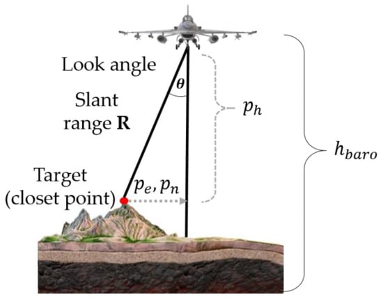
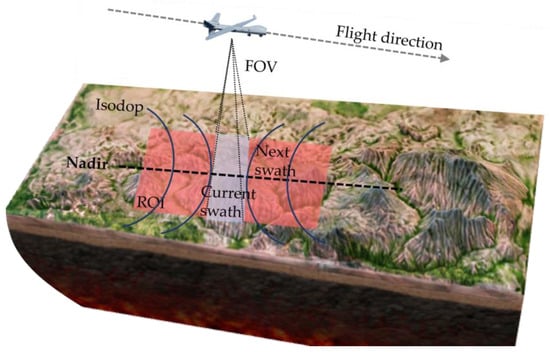
The major factors that affect TRN performance are terrain roughness, sensor reliability, and filter design. The performance of TRN is highly dependent on terrain roughness, as a higher degree of roughness guarantees better navigation performance. Likewise, sensors that provide accurate terrain information can achieve better navigation performance. Thus, this study uses an interferometric radar altimeter (IRA) to obtain terrain information. The IRA is known that to be able to extract precise three-dimensional terrain information based on synthetic aperture radar (SAR) interferometry technology. Since conventional radar altimeters (RA) estimate altitude as straight vertical distance, they cannot be used in high altitudes because of their footprint issue. On the contrary, the accuracy of IRAs is not diminished at high altitudes, allowing for a diverse operation range. These advantages have led Honeywell to apply IRA-equipped TRN systems to Tomahawk cruise missiles [3]. The IRA used in this study extracts three-dimensional ground coordinates with three antennas. By using three antennas, a multi-baseline is available which can compensate for ambiguity in the wrapped phase [4]. In addition, digital signal processing [4] and effective look angle calculation [5] are introduced in order to achieve more precise terrain information. Despite these efforts, some IRA uncertainties caused by geometric factors and IRA-inherent measurement errors remain. These uncertainties contaminate IRA outputs, crucially impacting the navigation performance of low-grade IRA sensors in particular. Unfortunately, since it is difficult to eliminate these uncertainties by signal processing, a robust filter is required to solve this issue. Various types of filters have been suggested to handle the uncertainty including the Extended Kalman filter (EKF), the unscented Kalman filter (UKF), the point mass filter (PMF) and the particle filter (PF). The PF, which was chosen for use in this study, estimates state based on a statistical approach using Monte Carlo simulation.
The basic idea of the PF is to represent the posterior density using random particles with associated weights. The key factors that affect PF performance are the accuracy of the system model, reliability of the measurement model, and degeneracy. The accuracy of the system model is determined by the hardware of the system. Likewise, the reliability of the measurement model is determined by the hardware of the sensors. Even though a good hardware system guarantees better navigation performance, there is a physical limitation to what these systems can achieve, and the cost would be prohibitive. Thus, in general, the PF performance pivots on the issue of degeneracy.
Degeneracy is an inherent risk of the PF. After a few iterations of particle propagation, only very few particles hold significant weight while the others have negligible weight. This phenomenon is referred to as sample degeneracy. This issue can be solved by increasing the number of particles, adopting proper proposal distribution, or implementing a resampling procedure. However, increasing the number of particles leads to an increase in computational burden, so it is not an appropriate solution for a real-time operating system. The adoption of proper proposal distribution does not yield significant improvement because it is dependent on classical sampling strategies [6]. Consequently, resampling strategies have become a popular way to diminish degeneracy in the PF. However, the resampling procedure introduces a new problem: sample impoverishment. Sample impoverishment occurs during the resampling process, which favors large weighted particles, resulting in the abandonment of particles with lower weights. This has a detrimental effect on particle diversity. Many resampling strategies have been suggested to alleviate this issue [6], including new resampling strategies using artificial intelligence [7,8,9,10,11]. Some of the algorithms that have been applied in resampling are the artificial fish swarm algorithm [7], the artificial immune system [8,9] and hybrid algorithms combining the artificial immune system and the evolutionary algorithm [10,11]. Some researchers have also suggested new estimators using the ant colony optimization algorithm (ACO) [12,13,14,15]. However, most of these attempts are either based on the general PF or have proven to be inadequate methods for TRN application. Thus, these algorithms require modification for use in TRN systems that utilize the auxiliary particle filter (APF).
Previously, the authors of this study developed a new immune auxiliary particle filter (IAPF) to enhance robustness. In doing so, we attempted to form a coherent process for achieving prime particle distribution. To achieve prime particle distribution, particles must be moved to the desired position. Generally, particles are moved in either a blind manner or a sighted manner. If a particle must move in a certain direction, it is called sighted; otherwise, it is called blind. The new immune particle filter using ant mutation proposed in the current study functions to indicate the parameters of the ant colony optimization (ACO) algorithm. The ACO algorithm moves particles to their most desirable positions in a sighted manner. This new mutation reduces the variance of the importance weight as compared to the APF and IAPF. Compared to the IAPF, the proposed algorithm also reduces computation time using two strategies: first, it implements a one-step ACO algorithm and second, it changes implementation order. The first strategy gives particles individual mutation intensity. In the previous IAPF, the mutation process is executed using regularized kernels, but as the size of the kernels cannot be individually adjusted for each particle, this approach is unable to guarantee the minimum variance distribution and therefore has proven to be ad-hoc. The second strategy enables consideration of the auxiliary variable. Since the IAPF activates the immune system once the APF algorithm has ended, the auxiliary variable is not effectively considered in the immune system. However, since our newly proposed filter implements the ant-mutated immune system after resampling is completed, the auxiliary variable becomes available for consideration.
This paper is organized as follows. In Section 2, we describe TRN and provide a detailed explanation of IRA sensor uncertainties. In Section 3, previous approaches are explained. Section 4 details the proposed ant-mutated immune particle filter. The efficiency of the proposed filter is verified via computer simulation in Section 5, and Section 6 concludes the work, highlighting its contributions to the field.
For the reader’s convenience, the acronyms used in this paper are listed in Table 1.

Table 1.
List of Acronyms.
3. Previous Approaches
3.1. Auxiliary Particle Filter
The particle filter represents prior and posterior distribution using random particles with associated weights. It is a sequential Monte Carlo method that employs the sequential estimation of relevant probability distribution using an importance sampling technique. The posterior distribution is expressed in terms of random measure.
where is the total number of particles, the delta function, the weighting factor, the sequence of all target states up to k, and the particle estimation value in time k. denote the set of state estimation and measurement through time k, respectively.
The solution of sequential importance sampling is represented in Equation (7). Posterior distribution becomes .
where represents the proposal importance distribution. Generally, the transition density is adopted as the proposal distribution, but since it does not inform current measurement, the proposal density cannot be optimized.
One technique for utilizing current measurement information is to use an APF. The key function of the APF is to imitate the operation of minimum variance importance distribution by utilizing auxiliary variables, which estimate empirical prediction distribution at time k − 1, giving the proposal the ability to adopt new data . APF reflects current measurement information by resampling particles at time k − 1 with available measurement information before particles are propagated through transition density. By resampling particles in the previous time step, APF favors particles that are likely to survive. These schemes have advantages in outlier performance and posterior tail performance, making the APF a better choice for TRN than the general PF. Stratified resampling is adopted in this study since it demonstrates better navigation performance than other resampling methods in the TRN system. The APF algorithm is the same as in [21].
The simple importance sampling of the PF and APF are basically the same algorithm, with one key difference lying in the choice of importance weight. The APF features which is more diffuse than due to the utilization of the current observation information. The knowledge of the current observation is incorporated into the proposal mechanism so that particles can move into the desired region. However, when there is an outlier, the distribution of the weights becomes uneven. This uneven distribution requires a large variance of the particle in order to approximate empirical density. In addition, poor-posterior tail performance poses a general problem for the importance sampling scheme. If a target distribution has a heavier tail than a proposal distribution, this could significantly increase the variance of estimation. In the case of the APF, the proposal distribution is adopted in terms of , with the importance weight becoming:
where and represent the likelihood function and transition function, respectively. This indicates that if the process contains severe nonlinearities or is contaminated by high process noise, then the point estimate using particles will not effectively represent the transition probability Consequently, the likelihood evaluation indicated by the transition density is not a wise choice for approximating the predictive likelihood. This could explain the poor performance of the APF algorithm.
3.2. Immune Auxiliary Particle Filter
Previously, the authors introduced an immune particle filter into the auxiliary particle filter scheme [9] to overcome such weaknesses. The immune auxiliary particle filter (IAPF) aims to enhance the robustness of the APF through the utilization of an immune system. The immune system distinguishes particles into three groups: alpha, neutral and omega. The alpha particles are superior particles considered to be significant contributions to the estimation performance, while omega particles are inferior particles that have negligible weights and are responsible for outliers. Neutral particles are neither alpha nor omega. The immune system consists of four major parts: affinity measure, confidence interval analysis, particle selection probability and hyper-mutation. Affinity refers to the interactions between antibodies or between an antibody and an antigen. Affinity measure calculates the proximity of particles to the true value. The distance from particle to true value is calculated based on a modified cell-line suppression method. After the affinity of the particles is measured, two fitness functions are defined: fitness function which evaluates the distance of particles and true value, and relative fitness function which describes the relativity of particle superiority. The confidence interval analysis takes on two roles in the immune system. One is to determine the survival of the omega particles. When the filter is not sufficiently converged or when the measurement has an outlier, the particles must be spread out. In this case, the immune system retains the omega particles in order to obtain diversity. The convergence of the filter is determined using a certain threshold . The other role of the confidence interval analysis is to tell which fitness function is more trustworthy using the parameter . The particle selection probability is expressed as follows.
Particles with high become alpha particles. Omega particles are designated as particles that have low . Since relative fitness exceeds the relativity of particle superiority and suppresses inferiority, particles with low are both relatively and absolutely inferior. The particles that are designated as neither superior nor inferior become neutral. After particles are assigned to each group, the immune system either eliminates or retains omega particles in accordance with the filter convergence. When the filter is sufficiently converged, omega particles are discarded, and randomly chosen alpha and neutral particles then become omegas and undergo the hyper-mutation process to maintain particle diversity. In the case when the filter is not sufficiently converged, the omega particles are retained for the hyper-mutation process. The hyper-mutation process is implemented using the kernel density estimator [22] from the regularized particle filter (RPF). Algorithm 1 describes the IAPF algorithm.
| Algorithm 1: Immune auxiliary particle filter (IAPF) |
| I. Initialize |
| II. Auxiliary weight update |
| Bootstrap posterior: |
| III. Stratified resampling |
| Repartition the interval into disjoint subinterval and draw independently in each of the subintervals for each iteration. |
| where, U is uniform distribution |
| Select indices using |
| draw index |
| IV. Rougheneing |
| V. Importance sampling proposal |
| VI. Weight update and normalization |
| VII. Posterior distribution |
VIII. Immune system
|
where the functions and represent the likelihood function and transition function, respectively. The details of the IAPF mechanism can be found in [9].
Even though the kernel estimator has certain advantages, it is biased, especially near the boundaries of the kernel. Furthermore, it is hard to optimize the bandwidth of the kernel. For instance, if the bandwidth is not large enough, dummy noise is produced in the tail of the estimate; if the bandwidth is too broad, it may lose its prime features due to over-smoothing. Although the mutation intensity can be adjusted using tuning parameters, it is certainly not enough. This calls for a new hyper-mutation process that can bring individual mutation intensity to each particle. For this reason, we have developed a new mutation based on ACO. The purpose of ant mutation is to achieve prime proposal distribution by utilizing individual mutation intensity, which brings better importance proposal than both the APF and IAPF. In addition, the new proposed ant-mutation algorithm introduces a one-step ACO algorithm for computational efficiency.
3.3. Ant Colony Optimization-Based Particle Filters
Ants are social insects whose priority is the survival of the colony as opposed to the survival of the individual. This behavior has provided the inspiration for new solutions to optimization problems. ACO, for example, was introduced by Dorigo in the early 1990s. ACO imitates the foraging behavior of ants. The goal of ants is to find the shortest path from the nest (starting position) to the food source (optimal solution). In ACO, this path selection is performed based on stochastic procedure using two parameters: the pheromone , and heuristic values. The pheromone indicates the probability of state transition, and the heuristic value acts as a problem-dependent quality measure. The ACO algorithm has been widely applied to various fields and problems such as the traveling salesman problem (TSP) [23], job shopping [24], communication networks [25], the bioinformatics problem [26], et cetera [27,28,29].
Since ACO works in a stochastic format, researchers have tried using it to develop new estimators [12,13,14,15]. In [12], ACO is integrated into the iterative unscented Kalman filter (IUKF) scheme for use as an iterative particle filter. Particles are propagated through the IUKF at the prediction step to obtain the state mean and covariance estimates . The ant direction is defined using transition and measurement probability and Gaussian distribution. The covariance of each ant indicates the pheromone value.
Another study [13] has suggested an ant stochastic decision-based particle filter for model-switching dynamic systems. In the study [13], ACO encapsulates model switching information by dividing particles into two model operations in a probabilistic manner. One is a pre-assumed model independent of new measurements and the other is related to new measurements. After particles are separated into each model, an ant-based resampling scheme is introduced to obtain better overlap with the true density function. Instead of ant travel, ACO is applied during the resampling step in order to sample the particles. The potential location of an ant becomes the probability of the ant to be sampled. The potential location is defined using the weights of particles.
ACO for the continuous Domain ) algorithm found in [14] has been utilized for abruptly and highly changing environments. This algorithm is different from the ACO algorithm. In the ACO algorithm, the artificial pheromone indicates an indirect information mechanism. The ant cooperates to build a probabilistic model on the pheromone deposition over the promising path (solutions). Based on this idea, builds a Gaussian mixture model for every state, using solution archive members. The new particles are drawn from created probabilistic models and evaluated using a fitness function.
Another ACO-based particle filter has been suggested by J. Zong [15]. This study aims to achieve a smaller Kullback-Leibler divergence (KLD) between the proposal distribution and the optimal distribution as compared to the generic PF by applying the ACO during the resampling step. Ants represent particles and move based on the route that leads towards the local peak of the optimal proposal distribution function. The optimal proposal distribution is defined as q. The basic movement is that of an ant moving with constant velocity, depositing pheromones along the path with constant enhancement. The initial value of the pheromones is equal to the particle weight:
The parameter is affected by every movement of the particles. The pheromone function on the paths belonging to the movement of particle is defined as follows:
where denotes the pheromone evaporation rate and is a constant enhancement value if parting j is located between the starting particle and the end point. The heuristic function is defined as the reciprocal distance between two particles (end point):
Now, the direction of ant movement is expressed by the following probability:
where parameter stands for the amount of pheromone and is the total number of particles. usually represents the heuristic value and its definition is dependent on the application. In addition, indicates the possible destinations of the ants. While an ant is traveling on the path, Equation (13) is used to identify the next path to be taken until potential solution paths have converged into an optimal solution. Equation (13) represents the probability of a particle selection particle among particles as the moving direction. The fitness function of each particle is proportional to the weight function, denoting the rate at which a particle is approaching the true state. The convergence of ACO is defined when the particle i re-locates to a closer proximity to particle j (the desired position), and . When this convergence is satisfied during each iteration then most particles will converge to this particle j. Thus, the termination condition of ACO becomes when particles tend to be around neighborhood regions with a high likelihood within a certain threshold. The threshold function is defined in Equation (14):
where is the weight of the target particle, randn is a random number generator from normal distribution and is the constant value. The details of the ACO-PF algorithm can be found in [15].
Although the above methods have been proven to be effective, it is hard to directly apply them to TRN systems using the APF and IAPF. First, since general navigation does not have a jump state, the studies in [12,13] are not adequate for TRN application. In addition, since both the APF and IAPF utilize the current measurement information in the auxiliary weight update, the algorithms used in [12,14] need to be modified for application to the APF and IAPF. Besides, the IRA often generates thick posterior tail distribution, making it risky to continue gathering particles near the high likelihood region. Consequently, a new ACO algorithm is required for the APF and IAPF schemes in TRN systems. The new proposed ACO for ant mutation utilizes a one-step, immune system- based ACO. The details of the proposed ACO algorithm will be discussed in Section 4.
4. Ant-Mutated Immune Particle Filter
4.1. Hyper-Mutation Process Based on ACO
A key characteristic of ACO is that ants communicate with each other using mutual information based on a stochastic decision. The mutual information indicates the suitability of the chosen path. In this sense, the ACO algorithm can be modified as shown in [14]. In the ACO-PF algorithm in [15], the weight of particles is used as the initial pheromone value, and the heuristic function denotes the distance between particles. During iteration, particles exceeding the threshold are relocated by updating ACO parameters. The proposed AMIPF combines the ACO algorithm with IAPF to bring individual mutation intensity. The immune system is used as an indicator of the ACO parameters, defining affinity in Euclidean distance using weights of particles and distance between particles and the estimation value. The x-axis of affinity measure is the particle location, and the y axis of affinity measure is defined using the likelihood function in Cartesian coordinates. This implies that the affinity measure contains the weight evaluation of particles (pheromones) and proximity evaluation between particles (heuristic value). The affinity measure is used to calculate the particle selection probability, which consists of two fitness functions that each considered the weight and proximity of particles in absolute and relative terms. This means that the particle selection probability can play a role as the probability function Consequently, the particles that have been separated using particle selection probability become the direction of ant movement. The ACO-PF aims to achieve minimum variance of the importance weights conditional on state history and measurement which functions under the same premise of the APF: operation of minimum variance of importance distribution. Hence, it is assumed that particles have already congregated in high likelihood regions during the auxiliary weight update step in the APF scheme. Consequently, the particle evaluation in the immune system implies the stochastic parameters of ACO during the last iteration. Since the ant movement and pheromone increments operate constantly in the aforementioned ACO-PF algorithm, the scheme can operate in a one-step procedure. For example, if ACO is converged after three iterations, it can be converged in one iteration by increasing the velocity threefold. Since the immune system determines the direction of ant movement and pheromone value, the only question remaining in a one-step ACO is that of how much the ants should move to reach the destination.
The premise of the proposed ACO is that there is an optimal path that can achieve the minimum variance of the importance distribution. Here, the optimal proposal refers to the minimum variance of the importance weights and can be differentiated from the optimal proposal, which can be defined in very restricted terms. Generally, the Kalman filter is known as an optimal estimator in a linear system where system and measurement noise are additive and Gaussian:
where and describe the system and observation, respectively. and . refer to the noise distribution of the system and the measurement and denote covariance of noise distribution. This can be reinterpreted by using Bayes rule which was discussed in [30]:
with . The system dynamics imply conditioning on This becomes the standard Kalman filter update for a prior with covariance. The weight in analytic expression becomes:
where the becomes the pdf for a Gaussian of mean and covariance . However, the noise distribution of the IRAs often forms the multimodal Gaussian distribution. Thus, the terminology optimal should be defined in different terms to include multimodal cases. The best solution path in ACO is considered to take Gaussian-like shape with minimum variance.
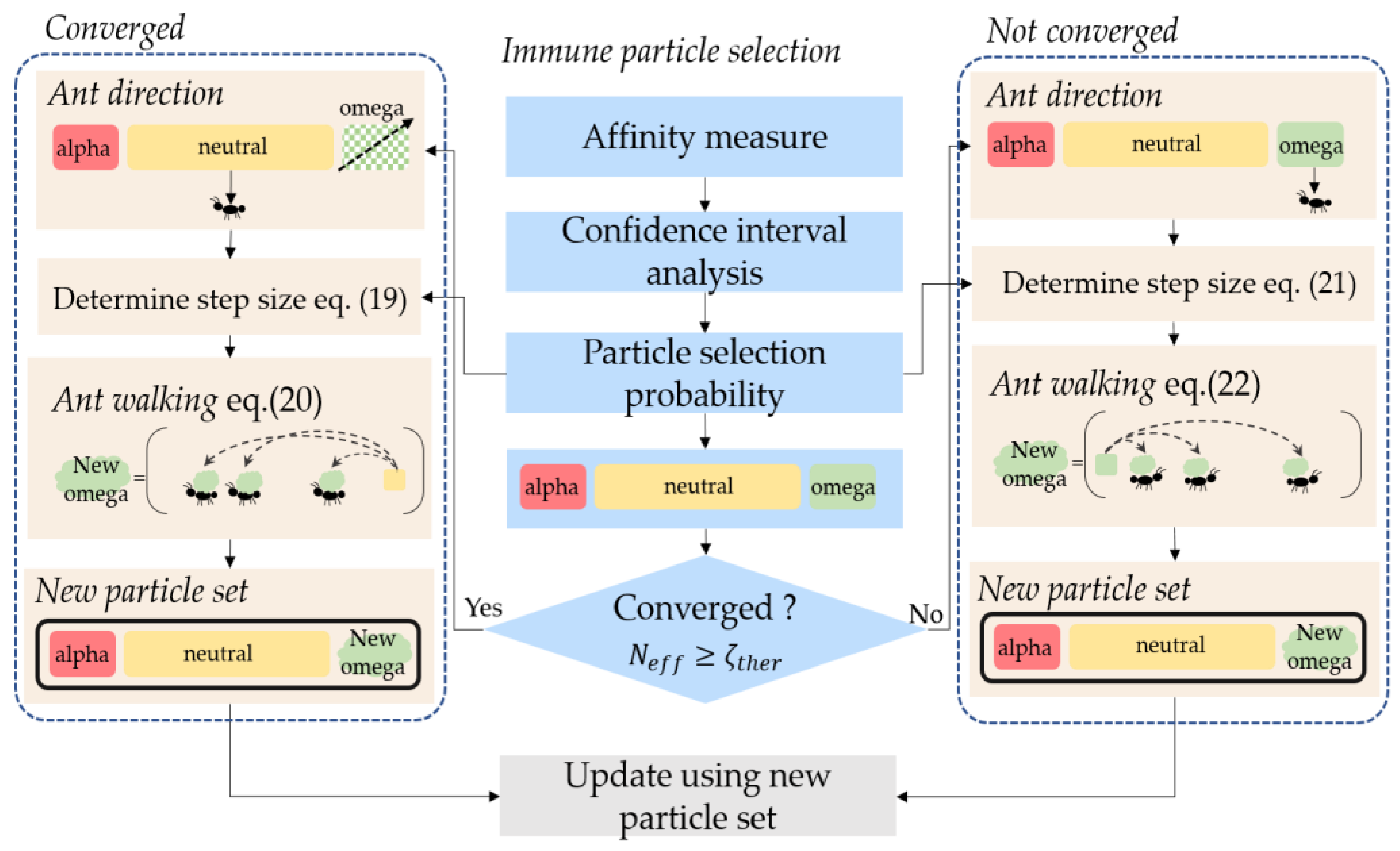
If previous particle filters based on ACO focused on locating the destination and path, the proposed algorithm focuses on the question of how much ants should move toward the designated destination on a certain path. The immune system determines the destination of the ants and ant movement based on filter convergence. If the filter is not converged enough, ants move toward inferior particles to obtain particle diversity; otherwise, ants move toward superior particles. Once the destination of the ants is defined, the proposed ACO starts to move ants to their desired position. The proposed ACO is mapped on space as where components in the original ACO, is the connected component path, and refers to the step size of the ant. The characteristics of the proposed ACO are described as follows
- There is an optimal solution .
- The immune system determines the parameters of ACO.
- The components are defined in the affinity measure domain, where is the number of components.
- The components evaluation is done within the immune system.
- The walking represents the path constructed by ant travel.
- The walking is determined once the destination of the ants is designated.
Given the above problem, the ants start to build the solution. In the case that the filter is already converged, the ants should be extracted from neutral particles , where is the number of ants. Then the ants start to walk toward their destination. As the proposed algorithm does not work iteratively, the step size variable is defined to work as the maximum number of iterations. The randomly chosen ants move toward the alpha particles based on their step size. The basic idea of step size determination is that the ant moves with constant velocity. For example, if the ACO is converged after three iterations with constant velocity, it can be assumed that the ACO can be converged in one iteration by increasing the velocity threefold. However, the constant velocity cannot provide individual mutation intensity, so other factors must be considered to induce individual velocity. Intuitively, particles with a high selection probability do not require high mutation intensity and vice versa. Based on this idea, the step size is defined as follows:
where is a tuning parameter for the step size and indicates the selection probability of selected neutral particles.
Now that the destination and the travel length have been determined, the walking function can be defined by the following equation.
where are the alpha particles.
The same rule is applied as when the filter is not sufficiently converged, except that now the omega particles participate in ant travel , where is the number of omega particles, which is the same as the number of ants. In this case, the purpose of the ants is to spread particles as far as they can in order to obtain particle diversity. Thus, the direction of the ant is oriented toward the location of the omega particles and beyond.
The walking function and the step size function are now slightly modified. Since the omega particles with low selection probability are already in charge of diversity, they do not need to move around, while omega particles with relatively high selection probability do. As a result, the particle selection probability of the omega particles is directly reflected in the step size function. The step size function reflects the selection probability of the omega particles and becomes the following:
where is a tuning parameter. For the ant’s destination, the opposite direction is taken and the distance between neutral particles and omega particles is reflected because it is the neutral particles that are in charge of adjusting particle distribution for the converged case. Since the population size of neutral particles differs from that of the omegas, some neutral particles are randomly chosen to move in order to match the population size , where o ∈ [1,. The walking for this is expressed as:
The proposed ant hyper-mutation process is illustrated in Figure 4 and summarized in Algorithm 2.
| Algorithm 2: The proposed ant-mutation algorithm. |
| Immune system: |
| The direction of ant |
| The final pheromone deposition |
| If |
| Extract ants from neutral particles |
| Moving ants to their desired position |
| Else |
| Extract ants from omega particles |
| Moving ants to their desired position |
| end |
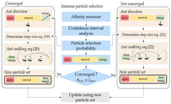
Figure 4.
Proposed ant-mutation scheme.
4.2. Ant-Mutated Immune Particle Filter Algorithm
The proposed AMIPF is developed to enhance the navigation performance and robustness of TRN systems using low-grade IRA sensors. The main purpose of the proposed AMIPF is to integrate a new mutation process using ACO into the IAPF scheme. While the IAPF moves particles in randomized directions, the proposed filter moves particles into the position which is considered the most desirable for each particle. The main idea of the new mutation process is to bring individual mutation intensity using the stochastic parameter from the immune system. The individual mutation intensity possesses an auto- tuning function based on the statistical measure. The statistical measure refers to the distance between the superior particles and inferior particles. If the likelihood function forms a low-peaked broad distribution, the distance between the superior and inferior particles becomes longer. If the likelihood function forms a high-peaked narrow distribution, the distance between superior and inferior particles becomes shorter. In this sense, the proposed algorithm executes the statistical auto-tuning mutation. Compared to the IAPF, which has several limitations including mutation intensity, the proposed filter enhances both navigation performance and robustness by using this auto-tuning scheme. For instance, where terrain has an unusually low level of roughness, the filter needs to spread particles as widely as it can. If the terrain recovers its roughness, the filter needs to congregate the particles into a high likelihood area. If the filter fails to spread particles properly, the filter loses its robustness. On the other hand, if the filter cannot congregate particles quickly enough, the estimation performance of the filter is degraded. In this sense, the proposed filter has a better ability to adjust particle distribution which leads to improve navigation performance as well as robustness.
Even though the auto-tuning scheme could lead to enhanced navigation performance and robustness, the computational cost must be considered before implementing ACO, since the maximum computational time for TRN update should be less than dozens of milliseconds [16]. Especially since the immune system already requires additional computational cost compared to the APF, there is not much computational room left for ACO. To deal with this issue, the proposed filter suggests two approaches: one is to implement the algorithm in a different order, and the other is to design a one-step ACO algorithm. For the first approach, the proposed filter implements the ant-mutation immune system scheme after resampling is executed. This has two advantages. First, it allows the auxiliary variable to be reflected in the immune system and second, it reduces the computational cost. Since the IAPF implements the immune system at the end of the APF scheme, it is unable to effectively utilize the auxiliary variable in the immune system. In addition, since particles with small weight are abandoned during resampling, there are fewer distinctive particles left to be evaluated in the immune system. However, the basic methodologies of the immune system remain the same as the IAPF regardless of implementation order. Thus, we will not provide further discussion on the matter in this paper. The computational complexity of each filter is the same as O(n). Since the APF, IAPF and AMIPF all originated from the particle filter, the computational complexity grows linearly with the number of particles. For instance, the APF can be represented as O(2n), since it utilizes two update processes for particles. In the case of the IAPF, the big O notation becomes O(3n) due to the affinity calculation for each particle. Finally, the proposed filter can be represented as O(3n − ). In the resampling step, the number of distinctive particles is reduced, which means the AMIPF has term since the abandonment of particles happens randomly rather than in an amortized way, so this does not reduce computational complexity. However, the most important aspect of computation time is the sampling rate of TRN. As mentioned above, the sampling rate of TRN is dozens of milliseconds, making the actual computation time for each run more important. If the average computation time for each run is reduced, this implies that the filter can be applied to navigation systems which require a higher sampling rate, such as missiles.
Heuristic algorithms require a sufficient number of iterations to find the solution. However, since the immune system already consumes computational cost, the algorithm which has a high compatibility with the immune system is required for particle movement. Since the immune system and ACO both utilize probabilistic decision-making, ACO can be simplified into a one-step procedure. Furthermore, ACO can infer the statistical measure in terms of travel length and move ants to their destinations using the immune indicator. For these reasons, ACO is better suited to the application. The reason that a one-step ACO mechanism is available is because the stochastic parameters required for ACO have already been obtained from the immune system. The principle of the one-step ACO is that ants travel the path with constant velocity. However, if every ant moves with constant velocity, it does not allow for optimal mutation intensity for each individual ant. Hence, other factors must be considered in ant movement. For one, the step size function reflects the particle selection probability: particles with high selection probability tend to maintain their original position, and particles with low selection probability tend to move forward into the desired position. Additionally, the statistical distance measure also takes part in individual mutation intensity. It indicates the distance from a particle to its destination which can be interpreted as the moving distance of an individual ant.
To summarize, the statistical distance measure and particle selection the probability take responsibility for individual mutation intensity and the tuning parameters and are in charge of determining the maximum number of iterations of ACO in this scheme. The entire proposed filter algorithm is depicted in Figure 5. The colors of the dots represent particle categories: red represents the alpha particles, yellow represents the neutral particles, and green represents the omega particles. Newly mutated omega particles are indicated by blue.
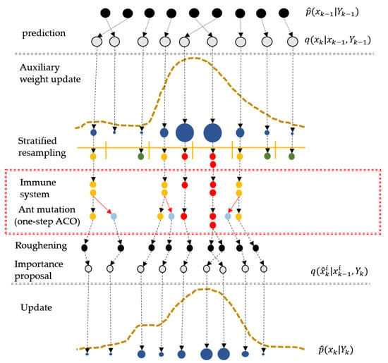
Figure 5.
Proposed filter scheme.
The most significant differences between the proposed filter and the IAPF are the implementation order of the proposed algorithm and the mutation methods. As shown in Figure 5, the proposed ant-mutated algorithm operates the immune system following the resampling step (marked in the red box) to utilize the auxiliary variable in the immune system. The IAPF cannot effectively have the auxiliary variable reflected in the immune system because the IAPF is applied after the APF algorithm takes place. As for the mutation method, the previous IAPF uses kernels to obtain particle diversity, while the proposed filter adopts the ACO algorithm. Since the original ACO algorithm requires a few iterations for convergence, the new one-step ACO algorithm was developed to save computation time. The entire algorithm of the proposed AMIPF is summarized in Algorithm 3.
| Algorithm 3: The proposed AMIPF algorithm. |
| I. Initialize |
| , |
| II. Auxiliary weight update |
| Bootstrap posterior: |
| III. Stratified resampling |
| Repartition the interval into disjoint subinterval and draw independently in each of the subintervals for each iteration |
| where, is uniform distribution. |
| Select indices using : |
| draw index |
IV. Immune system
|
| V. Ant-mutation (Table 3) |
| VI. Roughening |
| VII. Importance sampling proposal |
| VIII. Weight update and normalization |
| IX. Posterior distribution |
where the functions and represent the likelihood function and transition function, respectively. The detailed mechanism of the immune system can be found in [9].
5. Simulation
5.1. Simulation Conditions
To verify the efficiency of the proposed particle filter, TRN simulation using a low-grade IRA sensor was conducted using the Monte Carlo (MC) simulation method. The simulation trajectories consist of two areas which come from actual terrain area; one holds valid overall roughness and the other has low roughness. The simulation trajectories are called as SIM1 and SIM2, respectively. The simulation parameters are presented in Table 2.

Table 2.
Simulation parameters.
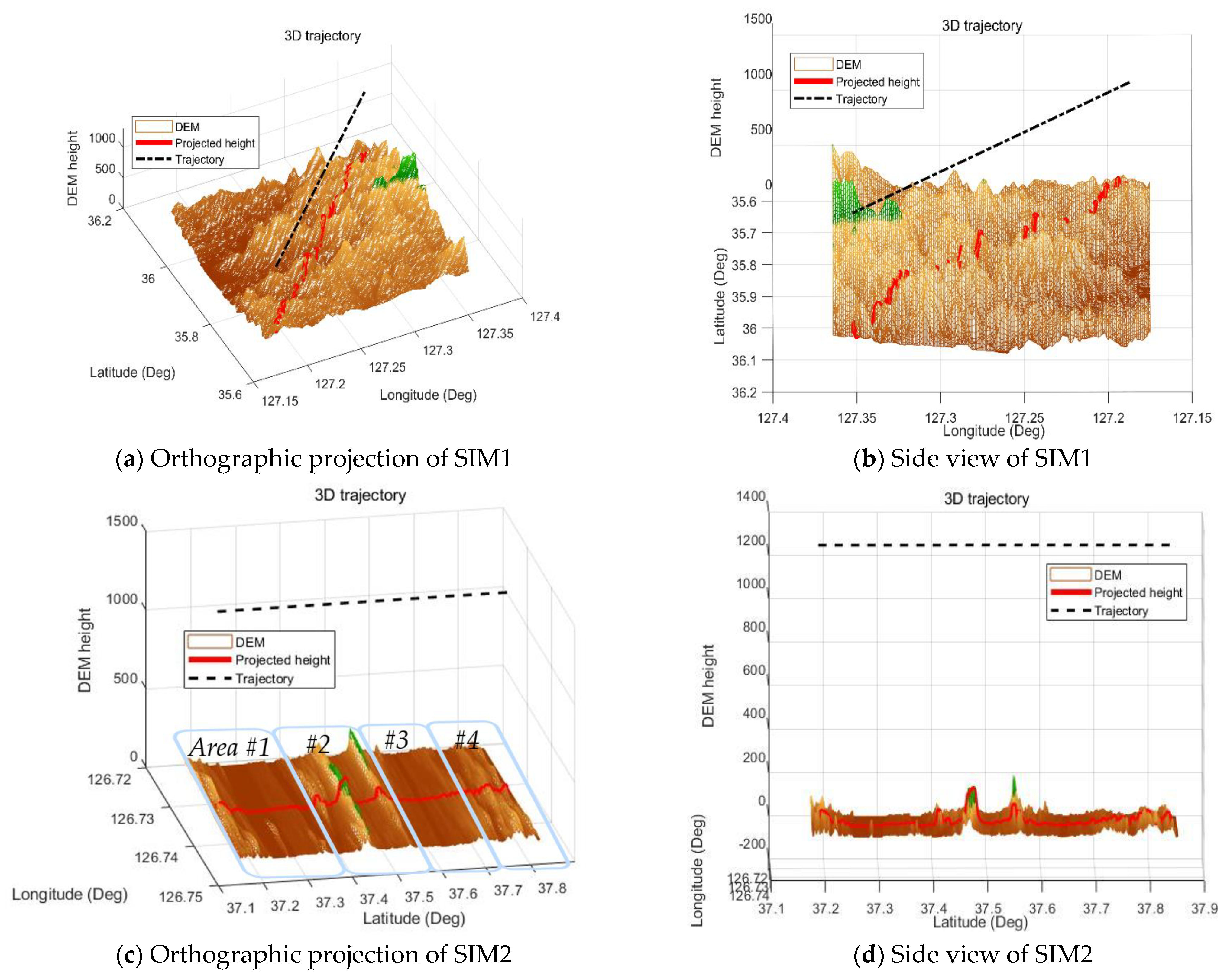
The simulation trajectories are depicted in Figure 6.
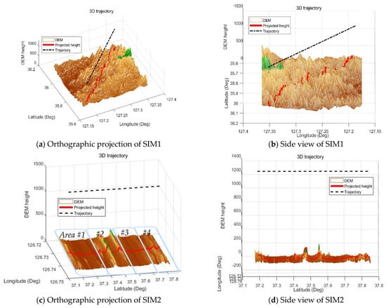
Figure 6.
Simulation trajectories. (a) Orthographic projection of SIM1. (b) Side view of SIM1. (c) Orthographic projection of SIM2. (d) Side view of SIM2.
Figure 6a,c depicts the orthographic projections of SIM1 and SIM2, while Figure 6b,d show the side view of each trajectory. The flight direction of SIM1 is diagonal, while the UAV in SIM2 travels in a latitudinal direction with a fixed longitude point. As mentioned in the introduction, the performance of TRN is highly dependent on terrain roughness. Terrain with a high degree of roughness can provide a distinctive target terrain point, which in turn can reduce the uncertainty of IRA measurements. However, if the roughness of the terrain is low or if the terrain is a repetitive, it is hard to accurately extract the nearest point, resulting in high uncertainty in the IRA output. The SIM1 trajectory is the referenced trajectory and holds valid overall terrain roughness. In this case, the APF works the best. On the contrary, the SIM2 trajectory, which has a low level of roughness overall trajectory, demonstrates the efficiency of the proposed filter. The SIM2 trajectory can be factorized in four areas. In Area #1 (~100 s), the terrain loses its roughness, recovering it in Area #2 (100~150 s) but dramatically losing its roughness again in Area #3 (150~230 s) before finally recovering it at the end of the trajectory (Area #4, 230~300 s).
5.2. Simulation Results
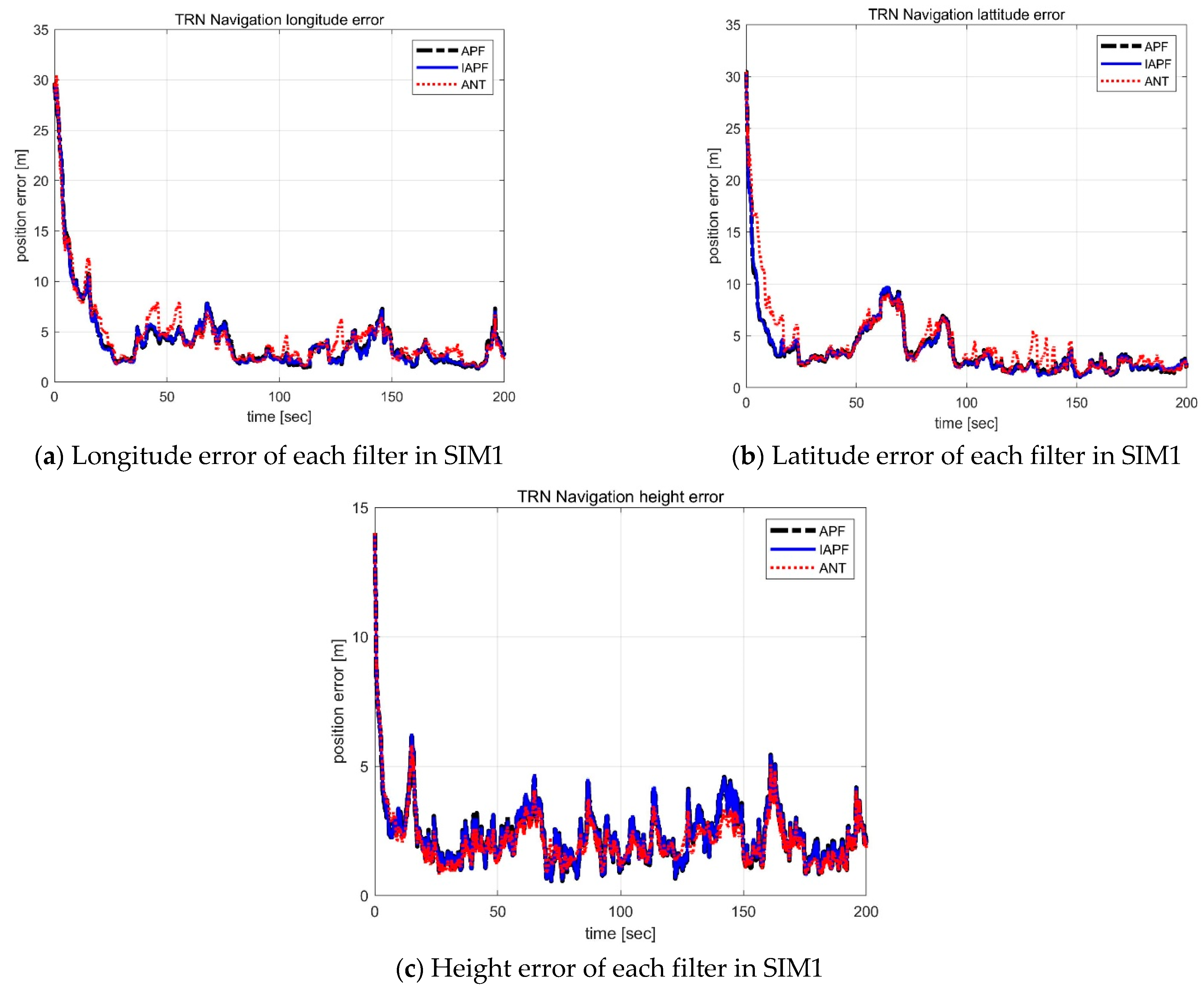
Figure 7 illustrates the SIM1 TRN results of the APF, IAPF, and the proposed filter labeled as AMIPF.
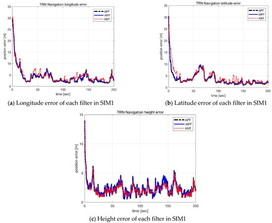
Figure 7.
The position error plot of each filter in SIM1. (a) Longitude error of each filter in SIM1. (b) Latitude error of each filter in SIM1. (c) Height error of each filter in SIM1.
In the referenced trajectory, there is no significant difference between the APF and IAPF. The proposed filter shows some peaks on the longitude axis in the 40~60 s and from 125~130 s as well as on the latitude axis from 128~140 s. For the terrain that has a high degree of roughness, the APF displays the best performance, while the other robust filters are degraded. This is because filters are required to have a tolerance for outliers in order to achieve robustness, which means that even in the best scenarios they can only provide suboptimal performance. However, both the IAPF and the proposed filter demonstrate robustness in SIM2, as depicted in Figure 8.
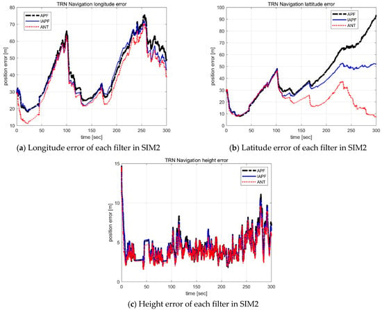
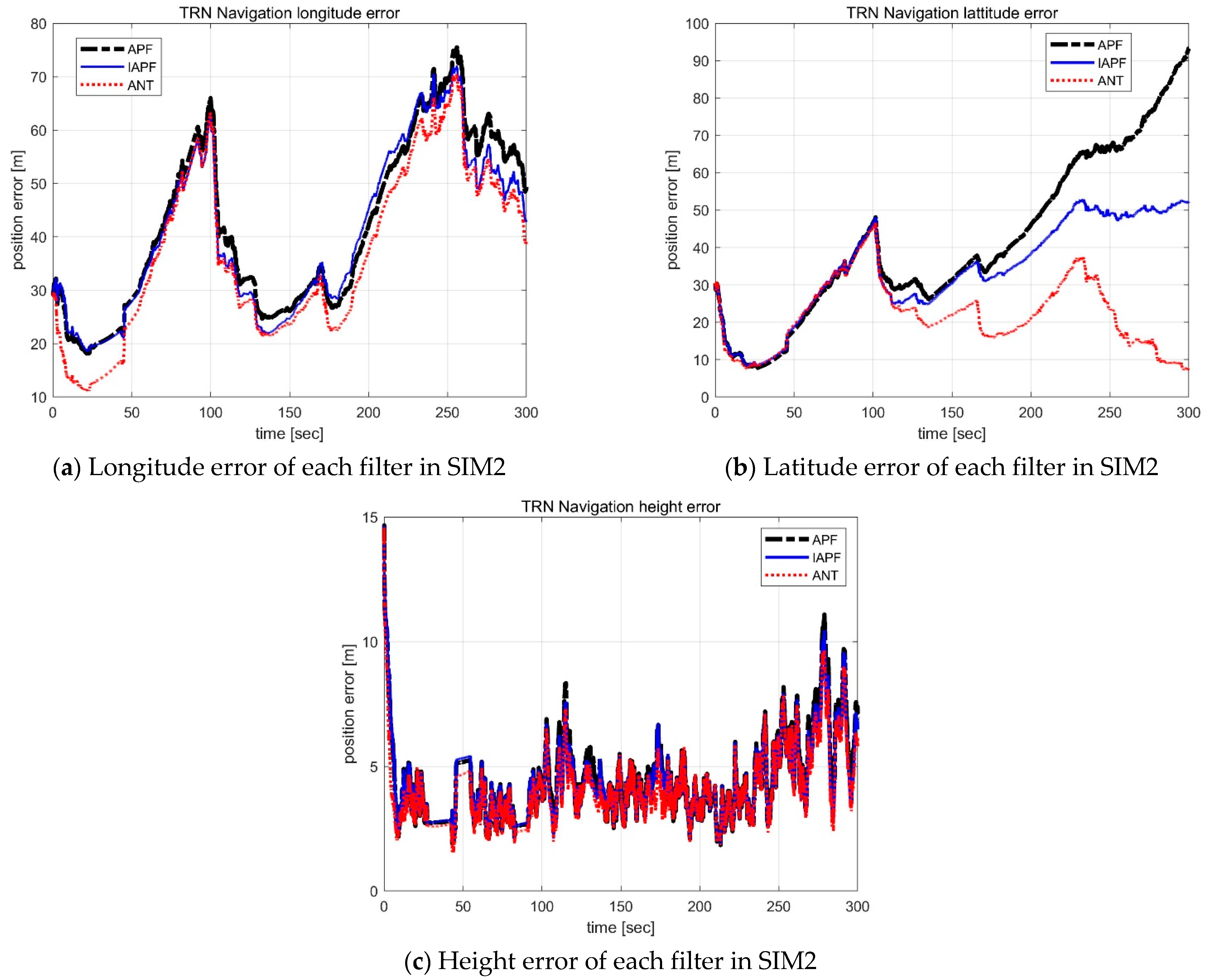
Figure 8.
The position error plot of each filter in SIM2. (a) Longitude error of each filter in SIM2. (b) Latitude error of each filter in SIM2, (c) Height error of each filter in SIM2.
As mentioned in the previous section, the terrain characteristics of SIM2 change along the flight trajectory, and the overall roughness of the entire trajectory is unusually low. This causes the APF to diverge, demonstrating the need for filters that possess strong robustness. Particularly on the latitude axis, the APF diverges and cannot recover its estimation performance. It is assumed that the flight direction of the UAV affects estimation performance. The IAPF, on the other hand, shows some tolerance but still not enough. The proposed AMIPF shows the best navigation performance in SIM2. The most significant improvement of the proposed filter can be seen in Area #4 where the roughness of the terrain is recovered. As terrain roughness is recovered, the estimation performance of the filter is expected to recuperate as well. However, the APF loses its estimation performance on the latitude axis. On the longitude axis, it seems that the APF recuperates its estimation performance. Similarly, the IAPF maintains its estimation performance on the longitude axis but cannot recover on the latitude axis, especially in Area #4. On the other hand, the proposed filter both maintains its estimation performance and promptly recovers it.
The comparison criteria of the horizontal position are determined using the two peaks shown in Figure 8. For the longitude axis, the first peak is in the 100 s (Area #2) and the second peak is in the 250 s (Area #3). For the latitude axis, the first peak is the same as the longitude, while the second peak in the 230 s (Area #3) serves as the comparison criteria. In Figure 8a, the IAPF shows improvement by 3.21 m on the first peak and 3.34 m on the second peak. In Figure 8b, there is no significant difference between the IAPF and the APF on the first peak but IAPF reduces its position error by 12.85 m on the second peak. In comparison, the proposed AMIPF outperforms the APF and IAPF on both axes. As shown in Figure 8a, the proposed filter reduces position error by 2.75 m on the first peak and 4.86 m on the second peak as compared to the APF. Compared to the IAPF, the proposed filter enhances navigation performance by 1.52 m on the second peak, but there is no significant improvement on the first peak. In Figure 8b, the position error of the proposed filter is reduced by 1.4 m on the first peak and 28.06 m on the second peak in comparison to the APF. Compared to the IAPF, the proposed filter shows 1.35 m and 15.21 m of improvement for the first and second peaks.
For the vertical position, there is no outstanding feature point that exists in Figure 8c, so the evaluation of filter performance is done via numerical method using probable error (PF).
Figure 9 shows the RMS results for 100 MC on SIM2. TRN 3 sigma indicates the covariance of particle distribution, or the coverage of the filter. The coverage should be wider on low roughness terrain and become narrower on high roughness terrain. As shown in Figure 9a, for two out of 100 simulations, the APF stays out of its range of coverage on the latitudinal axis and cannot recover its estimation performance. The IAPF result also exceeds its coverage on the latitudinal axis in one of the simulations. In the meantime, the proposed filter stays within its range of coverage on both horizontal axes. In addition, the TRN 3 sigma of each filter differs in width. The APF displays the narrowest width for the overall simulation time. This means that the APF cannot exploit its diversity when the terrain roughness gets lower, as shown in Figure 9. Both IAPF and the proposed filter have wider coverage than the APF. However, in Area #4 where the roughness of the terrain becomes higher, the IAPF becomes wider than the proposed filter. These results indicate that the proposed filter possesses a better and faster ability to adjust its particle distribution and maintain the minimum variance. The performance of each filter is represented as circular error probability (CEP) for horizontal position error and probable error (PE) for vertical position error, which are measures of a weapon system’s precision. The total CEP errors of the APF, IAPF and proposed filter are compared in Table 3 and The PE errors of each filter are compared in Table 4.
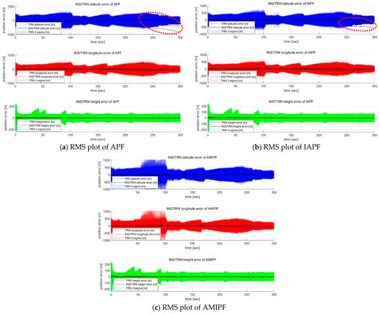
Figure 9.
RMS plot of each filter on SIM2. (a) RMS plot of APF. (b) RMS plot of IAPF. (c) RMS plot of AMIPF.

Table 3.
Horizontal position error (CEP).

Table 4.
Vertical position error (PE).
Although, there is performance degradation on the proposed filter for the horizontal position in SIM1, the position error is significantly reduced in SIM2. Compared to the APF, the proposed filter shows 16.3710 of improvement. Compared to the IAPF, the AMIPF enhances navigation performance by 9.3983 m. For the vertical position, the proposed filter shows the best performance. In addition, the computation cost of the proposed filter is lower compared to that of the IAPF. The average computation time for each run is measured using MATLAB 2017b with Intel® Xenon CPU e5-2620 v.4 @2.1 GHz, 64 bit, 64 RAM. In this condition, the average computation time for each filter is denoted in Table 5.

Table 5.
Average computation time.
6. Conclusions
This study introduces a new particle filter to improve the robustness and navigation performance of TRN systems that utilize low-grade IRAs. The new particle filter combines the immune auxiliary particle filter and ant colony algorithm so that the immune system discriminates inferior particles from superior particles using a stochastic procedure which then indicates the ACO parameters. Using such indications, a one-step ACO algorithm moves ants into the most desirable position for mutation. This new form of mutation achieves a smaller variance of importance weight than the APF and IAPF. In addition, the ant movements contain a statistical auto-tuning feature which possesses the ability to combat outlier and thick posterior tail distribution. These two properties result in the enhancement of estimation performance and robustness. The efficiency of the proposed filter is verified via TRN simulation applied to a UAV. The proposed filter shows significant improvement in navigation performance and robustness on low roughness terrain areas compared to both the APF and IAPF. The proposed filter also reduces computation time compared to the IAPF.
The future development of the study could be extended to the searching mode of TRN which estimates position in the case of the large initial position error of a few kilometers. The current study is based on the tracking mode of TRN, which estimates the precise position. In order to be applicable to the searching mode, the algorithm must possess an extensive exploration ability to locate a candidate terrain point to track over a broad area. To tackle that problem, the searching space of the proposed algorithm will need to be redirected.
Author Contributions
Conceptualization, S.K. and M.-J.Y.; methodology, S.K.; software, S.K.; data curation, S.K.; writing—original draft preparation, S.K.; writing—review and editing, S.K. and M.-J.Y.; supervision, M.-J.Y.; Both authors have read and agreed to the published version of the manuscript.
Funding
This research received no external funding.
Institutional Review Board Statement
Not applicable.
Informed Consent Statement
Not applicable.
Conflicts of Interest
The authors declare no conflict of interest.
References
- Sun, R.; Zhang, W.; Zheng, J.; Ochieng, W.Y. GNSS/INS Integration with Integrity Monitoring for UAV No-fly Zone Management. Remote Sens. 2020, 12, 524. [Google Scholar] [CrossRef]
- Hasheminasab, S.M.; Zhou, T.; Habib, A. GNSS/INS-Assisted Structure from Motion Strategies for UAV-Based Imagery over Mechanized Agricultural Fields. Remote Sens. 2020, 12, 351. [Google Scholar] [CrossRef]
- Siouris, G.M. Missile Guidance and Control Systems; Springer Science & Business Media: New York, NY, USA, 2004; pp. 524, 551–576. [Google Scholar]
- Lee, D.-T.; Jung, H.-S.; Yoon, G.-W. An Efficient Interferometric Radar Altimeter (IRA) Signal Processing to Extract Precise Three-dimensional Ground Coordinates. Korean J. Remote Sens. 2011, 27, 507. [Google Scholar] [CrossRef]
- Oh, J.; Sung, C.-K.; Lee, J.; Lee, S.W.; Lee, S.J.; Yu, M.-J. Accurate Measurement Calculation Method for Interferometric Radar Altimeter-Based Terrain Referenced Navigation. Sensors 2019, 19, 1688. [Google Scholar] [CrossRef] [PubMed]
- Li, T.; Bolic, M.; Djuric, P.M. Resampling Methods for Particle Filtering: Classification, implementation, and strategies. IEEE Signal Process. Mag. 2015, 32, 70. [Google Scholar] [CrossRef]
- Ye, T.; Chen, L.; Wang, Z.; Tao, L. Artificial Fish Swarm Algorithm-Based Particle Filter for Li-Ion Battery Life Prediction. Math. Probl. Eng. 2014, 2014, 564894. [Google Scholar] [CrossRef]
- Han, H.; Ding, Y.; Hao, K. A new immune particle filter algorithm for tracking a moving target. In Proceedings of the 2010 Sixth International Conference on Natural Computation, Yantai, China, 10–12 August 2010; pp. 3248–3252. [Google Scholar] [CrossRef]
- Kang, S.; Han, K.J.; Yu, M.-J. Robust immune particle filter design for terrain-referenced navigation with interferometric radar altimeter. IET Radar Sonar Navig. 2020, 14, 1402–1409. [Google Scholar] [CrossRef]
- Han, H.; Ding, Y.; Hao, K.; Liang, X. An evolutionary particle filter with the immune genetic algorithm for intelligent video target tracking. Comput. Math. Appl. 2011, 62, 2685–2695. [Google Scholar] [CrossRef]
- Feng, J.; An, R.; Sun, Y. Immune Evolution Particle Filter for Soil Moisture Data Assimilation. Water 2019, 11, 211. [Google Scholar] [CrossRef]
- Wang, F.; Lin, B.; Li, X. An ant particle filter for visual tracking. In Proceedings of the 2017 IEEE/ACIS 16th International Conference on Computer and Information Science (ICIS), Wuhan, China, 24–26 May 2017; pp. 417–422. [Google Scholar] [CrossRef]
- Xu, B.; Zhu, J.; Xu, H. An ant stochastic decision-based particle filter and its convergence. Signal Process. 2010, 90, 2731–2748. [Google Scholar] [CrossRef]
- Heris, S.M.L.; Khaloozadeh, H. Ant Colony Estimator: An intelligent particle filter based on ACOR. Eng. Appl. Artif. Intell. 2014, 28, 78–85. [Google Scholar] [CrossRef]
- Zhong, J.; Fung, Y.-F. Case study and proofs of ant colony optimisation improved particle filter algorithm. IET Control Theory Appl. 2012, 6, 689–697. [Google Scholar] [CrossRef]
- Lee, J.; Sung, C.-K.; Oh, J.; Han, K.; Lee, S.; Yu, M.-J. A Pragmatic Approach to the Design of Advanced Precision Terrain-Aided Navigation for UAVs and Its Verification. Remote Sens. 2020, 12, 1396. [Google Scholar] [CrossRef]
- Park, J.; Kim, Y.; Bang, H. A new measurement model of interferometric radar altimeter for terrain referenced navigation using particle filter. In Proceedings of the 2017 European Navigation Conference (ENC), Lausanne, Switzerland, 9–12 May 2017; pp. 57–64. [Google Scholar] [CrossRef]
- Lee, J.; Bang, H. Radial basis function network-based available measurement classification of interferometric radar altimeter for terrain-aided navigation. IET Radar Sonar Navig. 2018, 12, 920–930. [Google Scholar] [CrossRef]
- Zhou, T.; Pheng, D.; Xu, C.; Zhang, W.; Shen, J. Adaptive particle filter basedo n Kullback-Leibler distance for underwater terrain aided navigation with muti-beam sonar. IET Radar Sonar Navig. 2018, 12, 433–441. [Google Scholar] [CrossRef]
- Ciuonzo, D.; Willett, P.K.; Bar-Shalom, Y. Tracking the tracker form its passive sonar ML-PDA estiamtes. IEEE Trans. Aerosp. Electron. Syst. 2015, 50, 573–590. [Google Scholar] [CrossRef]
- Candy, J.V. Bayesian Signal Processing: Classical, Modern and Particle Filtering Method, 2nd ed.; John Wiley & Son, Inc.: Hoboken, NJ, USA, 2009; pp. 237–289. [Google Scholar]
- Zabom, A.Z.; Ronaldo, D. A review of Kernel Density estimation with application to Econometrics. IER 2013, 5, 20–42. [Google Scholar]
- Yang, J.; Shi, X.; Marchese, M.; Liang, Y. An ant colony optimization method for generalized TSP problem. Prog. Nat. Sci. 2008, 18, 1417–1422. [Google Scholar] [CrossRef]
- Chaouch, I.; Driss, O.B.; Ghedira, K. A Modified Ant Colony Optimization algorithm for the Distributed Job shop Scheduling Problem. Procedia Comput. Sci. 2017, 112, 296–305. [Google Scholar] [CrossRef]
- Zhao, D.; Luo, L.; Zhang, K. An improved ant colony optimization for the communication network routing problem. Math. Comput. Model. 2010, 52, 1976–1981. [Google Scholar] [CrossRef]
- Duc, D.D.; Dinh, P.T.; Vu, T.N.A.; Nguyen, L.-T. An Efficient Ant Colony Optimization Algorithm for Protein Structure Prediction. In Proceedings of the 2018 12th International Symposium on Medical Information and Communication Technology (ISMICT), Sydney, Australia, 26–28 March 2018; pp. 1–6. [Google Scholar] [CrossRef]
- Shmygelska, A.; Hoos, H.H. An ant colony optimisation algorithm for the 2D and 3D hydrophobic polar protein folding problem. Bioinformatics 2005, 6, 30. [Google Scholar] [CrossRef] [PubMed]
- Falaghi, H.; Haghifam, M. ACO Based Algorithm for Distributed Generation Sources Allocation and Sizing in Distribution Systems. In Proceedings of the 2007 IEEE Lausanne Power Tech, Lausanne, Switzerland, 1–5 July 2007; pp. 555–560. [Google Scholar] [CrossRef]
- Al-Ruzouq, R.; Shanableh, A.; Barakat, A.; Gibril, M.; AL-Mansoori, S. Image Segmentation Parameter Selection and Ant Colony Optimization for Date Palm Tree Detection and Mapping from Very-High-Spatial-Resolution Aerial Imagery. Remote Sens. 2018, 10, 1413. [Google Scholar] [CrossRef]
- Doucet, A.; Godsill, S.; Andrieu, C. On sequential Monte Carlo sampling methods for Bayesian filtering. Stat. Comput. 2000, 10, 197–208. [Google Scholar] [CrossRef]
Publisher’s Note: MDPI stays neutral with regard to jurisdictional claims in published maps and institutional affiliations. |
© 2021 by the authors. Licensee MDPI, Basel, Switzerland. This article is an open access article distributed under the terms and conditions of the Creative Commons Attribution (CC BY) license (https://creativecommons.org/licenses/by/4.0/).

