An Analysis of Vertical Crustal Movements along the European Coast from Satellite Altimetry, Tide Gauge, GNSS and Radar Interferometry

Abstract

The main aim of the article was to analyse the actual accuracy of determining the vertical movements of the Earth’s crust (VMEC) based on time series made of four measurement techniques: satellite altimetry (SA), tide gauges (TG), fixed GNSS stations and radar interferometry. A relatively new issue is the use of the persistent scatterer InSAR (PSInSAR) time series to determine VMEC. To compare the PSInSAR results with GNSS, an innovative procedure was developed: the workflow of determining the value of VMEC velocities in GNSS stations based on InSAR data. In our article, we have compiled 110 interferograms for ascending satellites and 111 interferograms for descending satellites along the European coast for each of the selected 27 GNSS stations, which is over 5000 interferograms. This allowed us to create time series of unprecedented time, very similar to the time resolution of time series from GNSS stations. As a result, we found that the obtained accuracies of the VMEC determined from the PSInSAR are similar to those obtained from the GNSS time series. We have shown that the VMEC around GNSS stations determined by other techniques are not the same.

1. Introduction

Vertical movements of the Earth’s crust are widely studied along the European coast, which provides a reference for comparing the obtained results. The movements of the Earth’s crust are significantly related to the maintenance and updating of coordinate systems, human activity, monitoring of flood hazards and changes in the mean sea level [1,2,3,4,5,6]. These movements are manifested by the horizontal and vertical displacement of tectonic plates [7]. Vertical plate tectonics are more difficult to determine, and they have both natural and sometimes anthropogenic causes [8]. Vertical movements of the earth’s crust are classified as relative or absolute (geocentric) movements, direct or indirect movements and point or surface movements. They can be determined based on measurements involving various techniques, including geometric levelling, global navigation satellite systems (GNSS), Doppler orbitography and radiopositioning integrated by satellite (DORIS), satellite laser ranging (SLR), synthetic aperture radar (SAR) and very long baseline interferometry (VLBI). Vertical movements determined with the use of different techniques in the same area may not be identical [9,10,11]. They may also differ for the same measuring technique [12]. These differences can be attributed to environmental and anthropogenic factors, the types of applied data [10] and the data compilation method.

Currently, vertical movements of the earth’s crust are most often determined as absolute (geocentric) movements directly in permanent GNSS stations [13]. The density of GNSS stations may vary for the different continents. Some stations are located on the coast near tide gauge stations (TG) and colocated with them. Absolute vertical movements of the Earth’s crust on the coast can be determined indirectly from satellite altimetry (SA) and tide gauge (TG) data [13,14].

Tide gauges are widely used to detect sea level changes along European coasts. Changes in sea level on the regional and global scale have been monitored with high accuracy based on satellite altimetry (SA) data since 1993 [15]. Satellite altimetry observations provide information about absolute sea level within a geocentric reference frame. In turn, TGs measure sea level relative to a land benchmark.

The difference between SA and TG observations is the geocentric vertical crust motion at the TG site; therefore, both sea level measurements are combined to assess vertical displacement at TG sites. In recent research, a combination of these measurements has been used to estimate vertical crust movements [10,16,17].

Collaborative elaboration of results from different measurement techniques can be done by interpolation or simultaneous data alignment. Both for the joint elaboration of the results and their mutual verification, it is necessary to provide information on the accuracy of the obtained vertical movements of the earth’s crust from individual measurement techniques. This fact is often neglected in the literature, which may lead to misinterpretation of the final results [18]. To obtain the accuracy at the assumed level for each of the techniques, it is sought to determine the optimal conditions that should be met by the time series. Therefore, for mareographic data, the series should be from several dozen to several hundred years long with a monthly resolution. Similarly, requirements are placed on the time series composed of altimetric data [19]. The areas were selected so that the mareographic data was at least 50 years old and, in places, even up to several hundred years. In the absence of such extensive series, the stations available with a shorter time interval were adopted, as was the SA data in the longest possible time interval. This allows the influence of the circulation of the moon’s nodes around the sun to be taken into account, which many researchers have overlooked.

In this study, vertical crust movement was investigated based on the differences between the time series of daily/monthly sea levels generated with the use of SA and TG data in each selected TG station on the European sea coast. The change trends in mean sea level were determined from TG observations and SA data in the European coastal zone.

Vertical crustal movements in nearby GNSS stations were also determined. GNSS time series should contain data from at least 3 years of the measurement period [20] (optimally it is 5 years) with daily resolution. GNSS data is at least 5 years old, and PPP compiled is to be unaffected by GNSS network alignment.

An InSAR analysis was carried out in GNSS sites based on the data obtained from a SAR-C sensor mounted on Sentinel-1A/B satellites for one frame of ascending orbits and one frame of descending orbits. The persistent scatterer InSAR (PSI) method supported the determination of deformation at coherent points on the ground over a long time interval [21]. Displacement values were estimated by reducing error sources related to temporal and geometrical decorrelation and atmospheric phase delay [22]. The following issues were taken into account to reliably assess the identified persistent scatterer (PS) points:

• The locations at which PS and GNSS data are measured do not coincide; therefore, spatial interpolation is required [9];
• Sentinel-1 data are not synchronised spatially, which means that their start and end times differ within each orbit.

Due to the different technical approach and the time-consuming nature of the calculations, few studies indicate the optimal nature of the time series generated from the PSInSAR data together with the actual accuracy assessment. Typically, these are series with low time resolution (one interferogram per year, quarter or month) in a 1-, 2- or 3-year time frame. Recently, the literature has shown a resolution of 290 interferograms over 5 years [18].

Our article uses an average of 110 interferograms for ascending satellites and 111 interferograms for descending satellites along the European coast for a selected 27 GNSS stations, which gives over 5000 interferograms in a 3-year time interval, providing a time resolution of nearly 1 week.

To compare the PSInSAR results against GNSS, an innovative procedure was developed: the workflow of determining the value of vertical movement velocities in GNSS stations based on InSAR data.

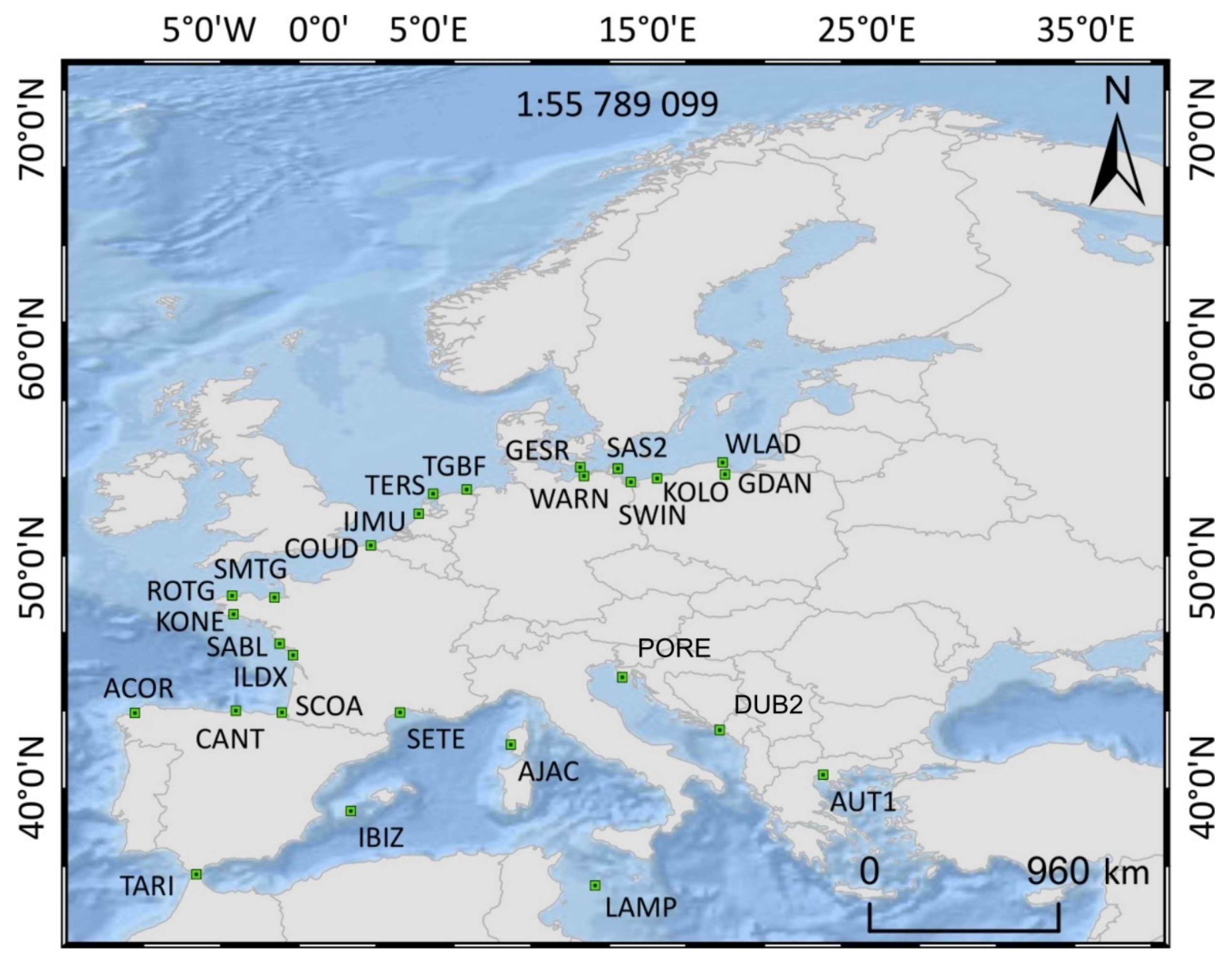
2. Materials and Methods

In this study, vertical movements of the earth’s crust along the European coast were estimated using tide gauge (TG), satellite altimetry (SA), GNSS and satellite interferometric synthetic aperture radar (InSAR) data (from Sentinel mission). Vertical movements were determined in the locations shown in Figure 1.

The obtained or created time series were decomposed. A linear trend and the trend standard error were determined. The linear regression method and Fourier analysis were used. Data were obtained from:

• Tide gauge (TG): Permanent Service for Mean Sea Level (PSMSL) (1856–2018);
• Institute of Meteorology and Water Management of the Polish National Research Institute (1951–2017 and 1993–2017);
• Satellite altimetry (SA): Copernicus Marine and Environment Monitoring Service (CMEMS) (1993–2017);
• SAR data (SAR): SENTINEL-1A/B data from the Copernicus Open Access Hub as part of the Copernicus mission (an initiative of the European Commission (EC) and the European Space Agency (ESA)) (2015–2017);
• GNSS: Nevada Geodetic Laboratory (NGL) (1999–2017); SONEL (1996–2018).

The absolute vertical crustal movement is calculated with the use of the following formula:

$$v_h=v_{SA}-v_{TG}$$

(1)

where v_SA—absolute change in sea level determined from altimetric data (referred to an ellipsoid); v_h—absolute vertical crustal movement (referred to an ellipsoid) and v_TG—relative change in mean sea level determined from TG observations.

The standard error in the determination of the absolute vertical movement of the Earth’s crust is given by the below formula:

$${\sigma }_{v_h}=\sqrt{{\sigma }_{v_{SA}^2}+{\sigma }_{v_{TG}^2}}$$

(2)

where σ_vh—the standard error of determination absolute vertical crustal movement; σ_vSA—the standard error of determination change in sea level determined from altimetric data and σ_vTG—the standard error of determination relative change in mean sea level determined from TG observations.

The calculated vertical movements of the Earth’s crust are verified against the values determined in neighbouring points with the use of other techniques, and the values are varied [23,24]. The basic prerequisite is the closest proximity of available TG [25,26]. The relative movements v_R between a GNSS station and a TG should be taken into account [27]. GNSS stations located on the coast provide the best neighbourhood. If GNSS stations are not available, vertical movements are determined at the nearest alternative points using SAR data. Deformations and deformation velocities are calculated based on SAR data [9,28,29], and they should closely correspond to the velocities determined based on GNSS station data.

Data from GNSS stations and TG form time series. SA and SAR data require additional processing to form a time series. The time series for each data set differ in time resolution (daily, several days, weekly, monthly), white and colour noise, a number of outliers and discontinuities (gaps and jumps). The quality of velocity calculations depends on the above factors, as well as the applied methods for eliminating or reducing the impact of undesirable factors.

Several approaches are used to detect and determine the jump value (vertical shifts in the data series) [30,31,32,33,34,35]. Jumping is caused by technical issues, human errors and environmental factors [33,36]. The determination of the vertical interval, which is regarded as a jump, poses the main technical problem. The vertical interval is difficult to determine because the ranks are affected by environmental conditions, as well as outliers and data gaps.

Several solutions for eliminating outliers have been proposed, and most of them are based on the assumptions presented in the literature [37,38]. Outliers are also eliminated by filling the gaps in the time series. Interpolation methods are used for this purpose [39]. Statistical and spectral methods are most commonly used to detect white and coloured noise [40,41]. In most cases, only the main annual and semiannual periods of seasonality are used, but considerably longer or shorter periods can also be applied due to the influence of other factors [27,42,43,44,45].

2.1. Analysis of Vertical Crustal Movement Velocities Based on SA and TG Data

Vertical crust movements in TG sites were estimated along the European coast based on different time series for SA minus TG (Equation (1)). The time series for SA and TG data describing changes in sea level were characterised by nearly identical behaviour. All the time series had seasonal components (annual, semiannual and 18.61-year cycles related to the relative movements of the Moon) and trend, which can be expressed as follows:

$$f_F\left(t\right)=a+bt+A_{a}cos \left({\omega }_{a}t-{\phi }_a\right)+A_{sa}cos \left({\omega }_{sa}t-{\phi }_{sa}\right)+A_{18.61}cos \left({\omega }_{18.61}t-{\phi }_{18.61}\right)$$

(3)

where f_F(t) is a Fourier function; a is the bias; b is the trend; t is time; A_a and A_sa are the annual and semiannual amplitudes, respectively; φ_a and φ_sa are the annual and semiannual phase, respectively; ω_a and ω_sa are the annual and semiannual angular frequency, respectively [46]; A_18.61 is the 18.61-year amplitude; φ_18.61 is the 18.61-year phase and ω_18.61 is the 18.61-year angular frequency.

The 18.61-year cycle is a lunar nodal cycle caused by the relative movements of the Moon. This important precession of the Moon, namely the 18.61-year lunar nodal cycle, causes tidal modulations over a range of interannual time scales. These modulations affect the interpretation of TG data spanning several years, particularly when dealing with water level extremes [47]. The least squares method was used to fit the time series of sea level variations for every station, and annual and semiannual amplitudes and the long-term trend in seasonal sea level variations were estimated.

TG measurements constitute long-time series of mean sea level data; they are obtained from the Permanent Service for Mean Sea Level (PSMSL) [48] and provide primary evidence for the rise in the globally averaged sea level. For this study, 27 TG stations on the European coast (Figure 1) were selected from the PSMSL [49] and the Institute of Meteorology and Water Management of the Polish National Research Institute. The TG data from the PSMSL are the time series of monthly averages from the Revised Local Reference (RLR) data set, and the 3 selected are presented in Figure 2. Data gaps in the time series were removed with the interpolation method. This series should not contain outliers, effects of seasonality or data discontinuities.

Gridded daily sea level anomalies with a resolution of 0.25 × 0.25 degrees and the time series for January 1993 to December 2017 from the Copernicus Marine and Environment Monitoring Service (CMEMS) were used. The time series of altimetric data (one series for each altimetric observation point) were obtained. This set combines data from several altimetry missions. Altimetric measurements were corrected for atmospheric effects (ionospheric delay and dry/wet tropospheric effects) and geophysical processes (solid, ocean, pole tides, loading effect of ocean tides, sea state bias and the inverted barometer response of the ocean). Detailed information on the introduced corrections can be found in AVISO [50] and CMEMS [51].

The differences in SA and TG data sets were investigated by correlation analysis. An SA grid point that was highly correlated with TG data was selected. It is simultaneously the closest SA grid to the TG data. The daily SA data were averaged to correspond with monthly TG data. The mean value of the correlation coefficient was 0.93.

The two main goals of the time series analysis are to describe the character of the analysed phenomenon based on a series of observations and to forecast future values. These goals can be achieved if time series elements are identified and described. The elements of a time series include a systematic component which can be described as a trend (linear or not) and a seasonal component where the duration of seasonal fluctuations can vary. Fluctuations can be regarded as a seasonality when their duration does not exceed 1 year, but when the corresponding period is longer, an economic cycle and a random component (noise) appear. These factors have to be identified in a formalised forecasting method. Periodic phenomena are identified in a harmonic analysis where a priori assumptions are not made. The harmonic analysis aims to decompose a time series with the use of cyclic factors on sine and cosine functions related to a given wavelength.

Harmonic analyses are performed to determine the average value of the studied phenomena. A trend was identified in the analysed data series; therefore, oscillations were determined with the use of the following model [46]:

$$f_H\left(t\right)=a+bt+{\displaystyle \sum }_{i=1}^{n/2}\left[a_{i}sin \left(\frac{2\pi }{n}it\right)+{\beta }_{i}sin \left(\frac{2\pi }{n}it\right) \right]$$

(4)

where f_H(t) is a harmonic function; a is the bias; b is the trend; t is time and n is the number of observations.

The amplitudes and phase shift were calculated for different harmonics. The annual, semiannual and 18.61-year harmonics were calculated. The annual, semiannual and 18.61-year harmonic functions for Sassnitz stations based on TG and SA time series are presented in Figure 3.

All-time series had a seasonal amplitude (annual, semiannual and 18.61-year cycle), and the correlations between the estimated amplitudes were calculated. The local sea level can be monitored with the use of altimetry and TG data, which can also be used to analyse the correlations between the variations in coastal sea level. The presented analysis focused on annual, semiannual and 18.61-year sea levels for 1993–2017, and altimetry and TG observations were compared on interannual timescales for validation purposes. SA and TG observations were characterised by a good fit in terms of the annual cycle, semiannual cycle and the 18.61-year cycle (Figure 4).

The correlation coefficient for annual variations from two independent observation techniques was determined at 0.92. The mean annual amplitude was ±5.59 cm with an estimation error of ±1.32 cm for TG data and ±6.17 cm for SA data with and estimation error of ±1.44 cm. The mean semiannual amplitude was ±2.57 cm with an estimation error of ±0.63 cm for TG data and ±1.79 cm for SA data with estimation error of ±0.42 cm. The correlation coefficient for semiannual variations was 0.72, which is a satisfactory result, but it was determined at only 0.34 for the 18.61-year cycle.

2.2. Analysis of Vertical Crustal Movement Velocities Based on GNSS Data

Vertical crustal movements can be classified as relative v_r or absolute v_h. Relative vertical crustal movements refer to any point (or surface) that is constant over time. Absolute vertical crustal movements are referred to an ellipsoid [52], and they comprise relative vertical crustal movements, average changes in sea level, eustatic movements and geoid changes over time. Absolute crustal movements are geocentric crustal movements [2] that are determined based on direct GNSS measurements as well as combined TG and SA measurements [13]. The location of a GNSS station relative to the TG station and the location of the point where changes in sea level were measured based on altimetric data have to be determined to compare the results generated by different methods.

The GNSS is commonly used for geodetic measurements because it monitors land movements with high precision [53,54]. This study analysed the measurements from a total of 27 GNSS stations that are colocated with or positioned in the proximity of a TG station on the European coast. The time series of vertical coordinates of 27 GNSS stations on the European coast (Figure 1) were obtained from the Nevada Geodetic Laboratory (NGL) [55] and SONEL (www.sonel.org, accessed on 12 December 2019). Time series from 3 selected GNSS stations from a total of 27 stations are shown in Figure 5.

The time series covered a period of 4 to 17 years with daily time resolution. The distance from the nearest TG ranged from 0.002 km to 16.069 km (Figure 6).

The data from the GNSS station form a daily time series covering several to more than 10 years. All the time series feature data discontinuities, jumps and noise. According to [13], the uncertainty of velocity calculations based on GNSS data ranges from 0.1 mm/year to 1.3 mm/year with a median of 0.21 mm/year. The time series of the coordinates from the GNSS station were decomposed. Missing values were filled by interpolation. Vertical shifts were defined with an algorithm developed for the needs of this study [32]. The VSED algorithm filters the outlier series with the Grubbs method. It defines and eliminates jumps and fits a trend line. The operations performed by the algorithm are presented in Figure 7.

The mathematical model used in this algorithm is a straight line with steps in different epochs:

$$h\left(t\right)=vt+h_0+c_1{s}_1+c_2{s}_2+\dots +c_m{s}_m$$

(5)

where t-epoch, h(t)—height difference in epoch t; v—velocity between stations; h₀—height difference at epoch 0; c₁, c₂, …, c_m—elements of the C matrix and s₁, s₂, …, s_m—magnitude of “jumps”.

The interval defining the “jump” was based on the standard deviation, which ranged from ±0.2 mm (values centred around the mean) to ±0.7 mm (values scattered around the mean). The number of jumps for the analysed GNSS stations, depending on the received height determination error, is shown in Figure 8.

The number of jumps does not affect the accuracy of height determination for individual epochs in the time series of coordinates from the GNSS station.

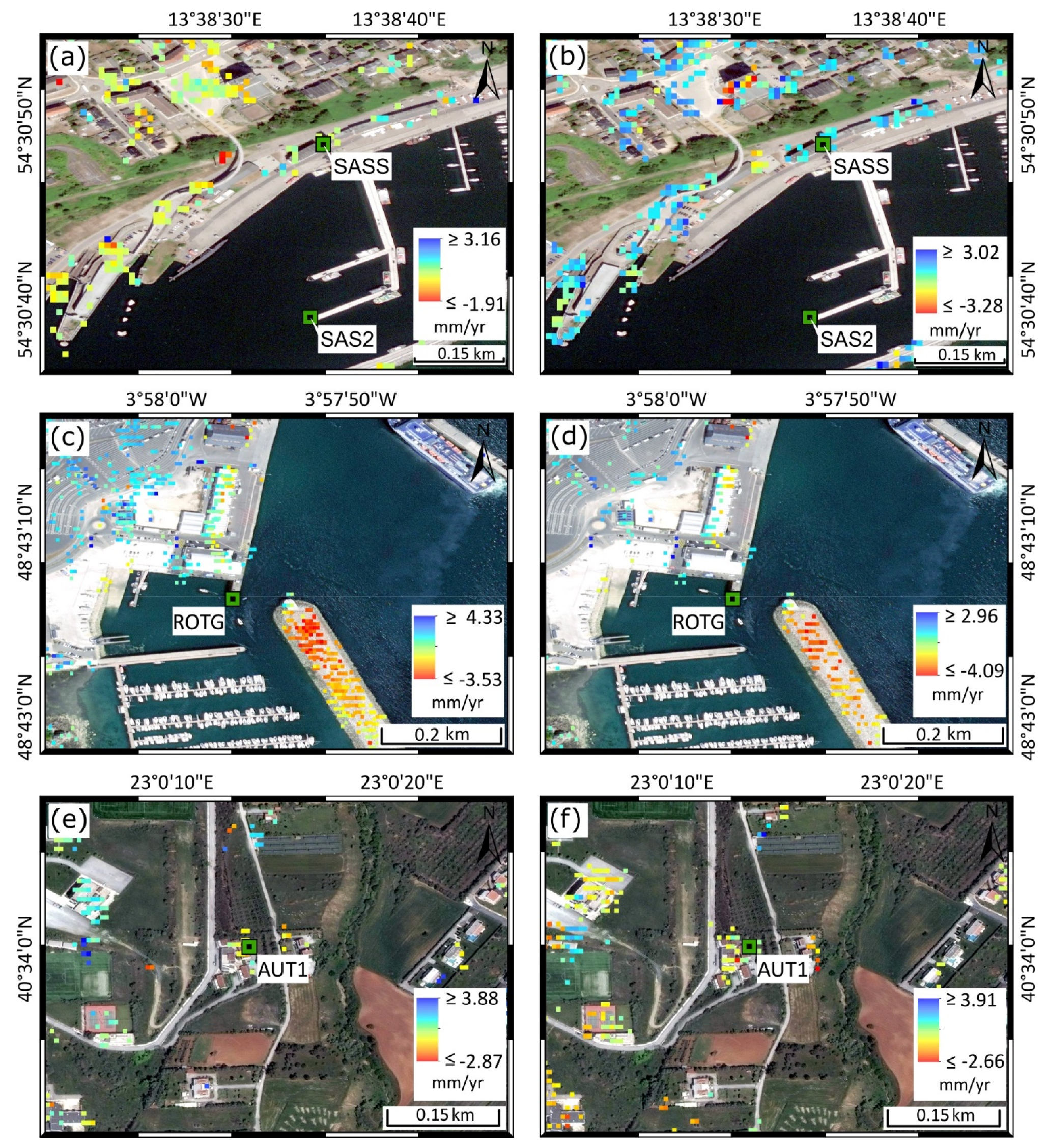
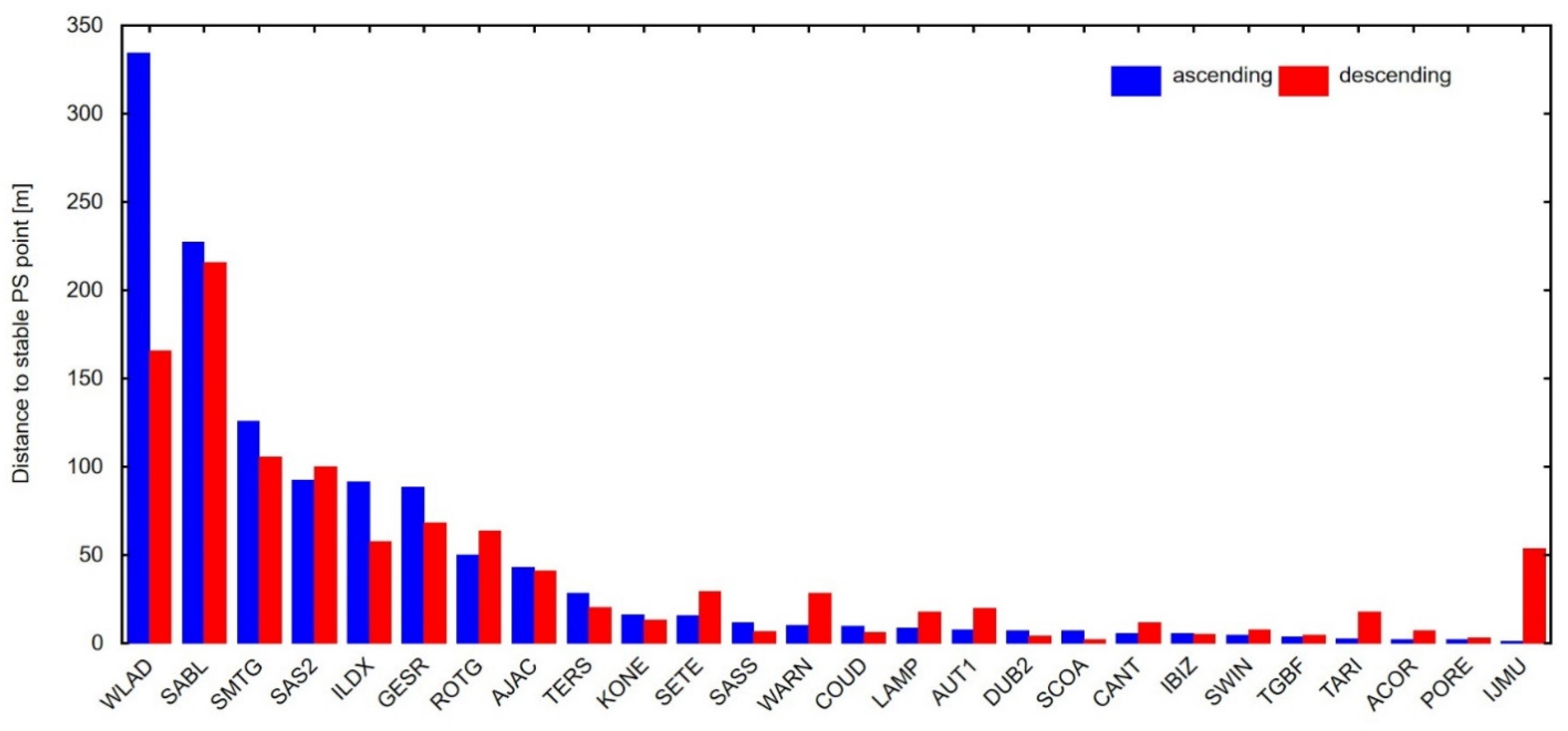
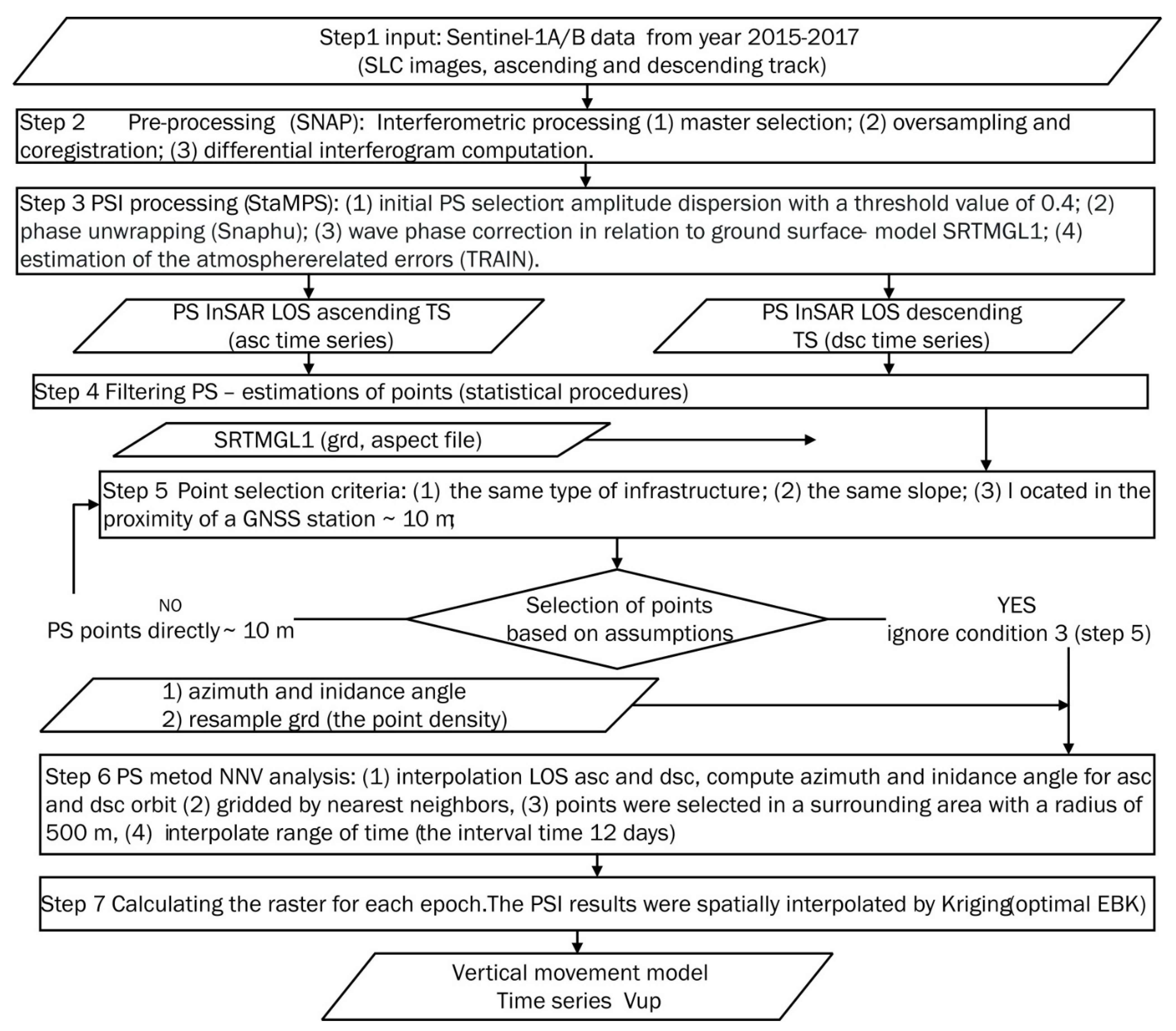
2.3. Analysis of the Vertical Movement Model Based on InSAR Data

The InSAR technique relies on interferometric comparison of SAR phase images to determine relative surface motions from the millimetre to centimetre [56,57,58]. In contrast to the pointwise information provided by GNSS, InSAR can provide a spatially dense image of surface displacements. The InSAR technique based on time series analysis (multitemporal InSAR, MTI) was used to achieve such a high level of accuracy and to reduce the basic error related to temporal and geometrical decorrelation and atmospheric phase delay. The course of deformation in the selected area was reconstructed with the use of point methods based on the selection of pixels that maintain coherence in time [21,59,60].

The interferometric phase in Equation (6) is the sum of contributions from several factors, including the components to be extracted, and it specifies ground deformation in the LOS (line of sight) direction in the time interval of the SAR image pair. The remaining factors relating to topography, atmosphere and orbit should be taken into account and eliminated from the interferometric phase.

$$\Delta {\phi }_{int}={\phi }_{defo}+{\phi }_{atm}+{\phi }_{orbit}+{\phi }_{topo}+{\phi }_{noise}$$

(6)

where φ_defo—LOS deformation, φ_atm—atmospheric delay, φ_orbit—orbit error, φ_dopo—DEM error and φ_noise—noise

The analysed GNSS stations are located in built-up areas along the European coast (Figure 1). The method StaMPS (Stanford Method for Persistent Scatterers), based on the PSI algorithm, was selected, and StaMPS software was used in this analysis. The PSInSAR algorithm detects stable scatterers and extracts phase information for these points. The StaMPS framework is a collection of spatial and temporal filtering routines that can be used to estimate the phase components in Equation (6) by assuming a spectral structure. More details are contained in [60]. The processed series of radar images (for 2015–2017) provided mean values of displacement velocities for persistent scatterers in the LOS direction (Figure 9). On average, a calculated 110 interferograms for ascending and 111 interferograms for descending orbital passes were determined at each point of the GNSS station.

Different objects make good permanent scatterers (PS), including buildings, lanterns and fragments of various structures (bridges, fences, etc.). In areas without infrastructure, rock outcrops, hard unvegetated earth surfaces and boulders can be used as PS points. However, the locations of PS points and GNSS stations do not coincide; the distances between selected PS points and the GNSS station are shown in Figure 10. The longest distance (of more than 300 m) was noted with the WLAD station, which is located on port breakwaters. The distance between PS points and ROTG, SCOA, ACOR and TARI stations, which are also located in the direct proximity of hydraulic structures, did not exceed 64 m. The distance between the PS point and the SABL was determined to be 227.34 m because it is the only GNSS station surrounded by a forest with no permanent structures in the vicinity.

The three-dimensional motion was only partly captured in the calculated rate of change in the LOS direction [61]. Therefore, the components of vertical movement had to be determined from SAR observations in the LOS. Radar satellites acquire image data of the same area on ascending (south to north) and descending (north to south) orbital passes. An LOS velocity V_los is composed of the 3D velocity components V_EW (East–West), V_NS (North–South) and V_up (Up-Down)_. The LOS displacements can be mathematically transformed to V_EW and V_up components if available at the same location for all analysed tracks and within the same time period. The V_NS displacements are small due to the polar orbit of all SAR satellites and the side-looking image geometry [62]. Various approaches to determining 3D surface motion from InSAR data are discussed in publications [63,64,65,66,67].

The PSI deformation value should be predicted at the location of the GNSS stations. Every location is different, and complex deformation phenomena may occur; however, an assessment of each station is possible [68]. In this article, vertical motion in GNSS stations was calculated based on various view geometries and viewing angles. During data postprocessing, ascending and descending PSI measurements were paired to calculate the vertical component for each PS point using Equation (7) [69]:

$$\left[V_{los}^{asc} V_{los}^{desc} \right]=A* \left[V_{up} V_{h_{ald}} \right]; A=\left[cos{\theta }^{asc} \frac{sin{\theta }^{asc}}{cos\Delta \alpha } cos{\theta }^{desc} sin{\theta }^{desc} \right]$$

(7)

where V_los—deformation along the LOS, V_up—vertical deformation, $V_{h_{ald}}$—projection of horizontal deformation in descending azimuth look direction, θ—incident angle and Δα—satellite heading difference between ascending and descending mode [22].

The scheme in Figure 11 shows the workflow of determining the vertical movement model based on InSAR data. In the scheme, in Step 4, groups of scatterers that exhibit similar behaviour are analysed. Statistical procedures are used to evaluate their spatial relationships and the consistency of estimated parameters in a given environment. During processing, many points are rejected based on different quality criteria [70].

The spatial distribution of ascending and descending PS point targets, in addition to the effect of temporal decorrelation, is highly related to the orientation of slopes and correlates well with the terrain aspect [61,64,71]. The proposed approaches included terrain aspect and interpolation performed in each range of time, both ascending and descending targets to be the same range time. The nearest neighbour vector (NNV) solution was used (according to the procedure http://gmt.soest.hawaii.edu, accessed on 10 January 2020). The PS points are not regularly spaced in space; the distances from their nearest neighbour with opposite geometry are different. Therefore, the search radius was determined based on the slope terrain analysis and the point density.

The locations of PS points and GNSS stations do not coincide; therefore, approaches were adopted according to the diagram shown in Figure 11. In the first approach (Step 5), the PS point was selected on the following assumptions:

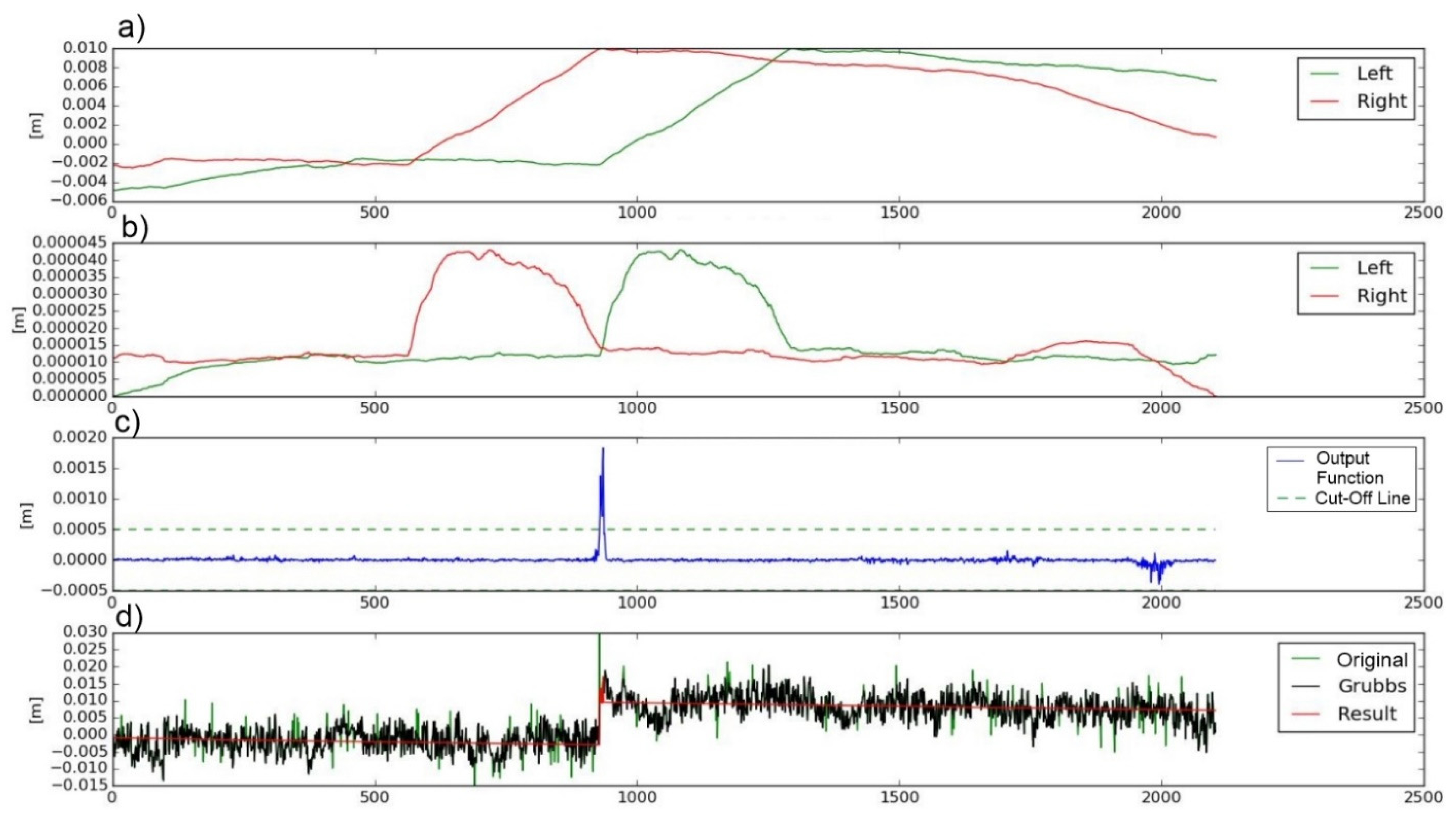
• The PS point is located on the same type of infrastructure or facility as the GNSS station. Sufficient PS points should be available to detect outliers. Next, the height of the PS points should be estimated to check whether the PS comes from the same technical infrastructure object and not from the surface level;
• Points should be selected from the area with the same slope. The point and slope heights were derived from data based on Shuttle Radar Topography Mission Global 1 arc second (SRTMGL1);
• PS point targets from ascending or descending tracks are located in the proximity of a GNSS station, ~10 m.

The PS points that met the criteria listed above were 25% of the points (6 stations) (Figure 10). In the second approach (Step 6), the following was adopted:

• There are no PS points directly (condition 3 from the first attempt);
• Points were selected in a surrounding area with a radius of 500 m;
• Eliminate outliers;
• Displacements behave linearly in time within a radius of 500 m of the GNSS station.

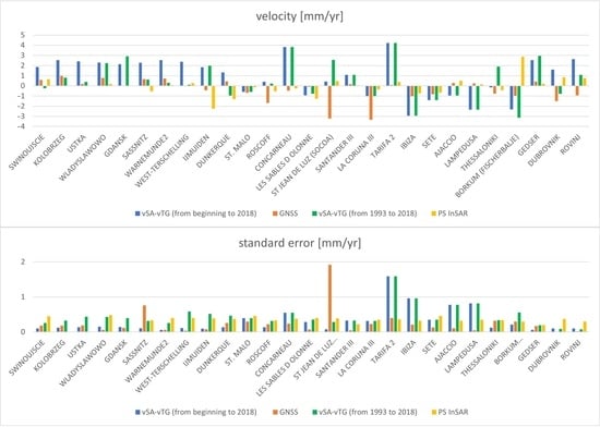
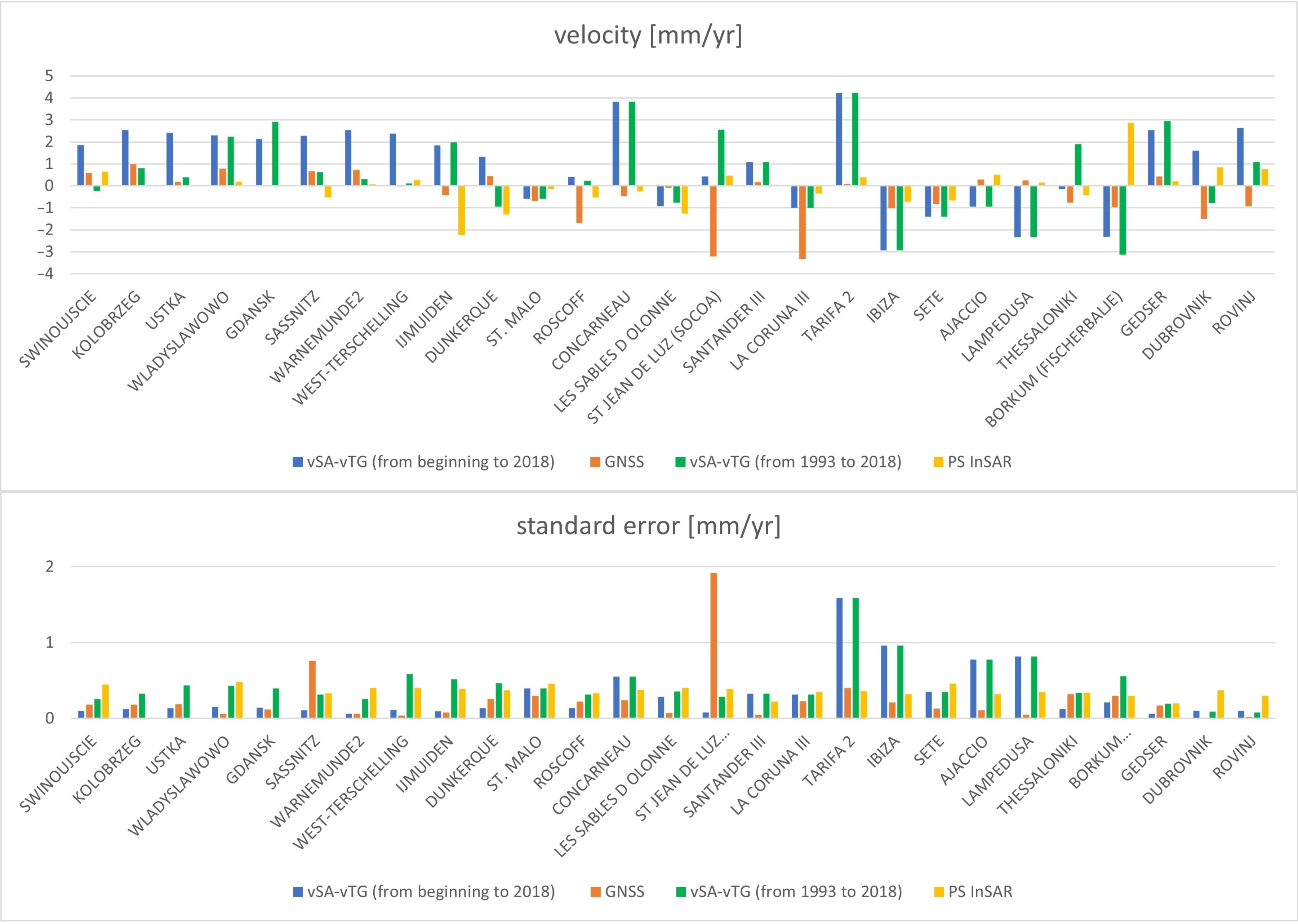
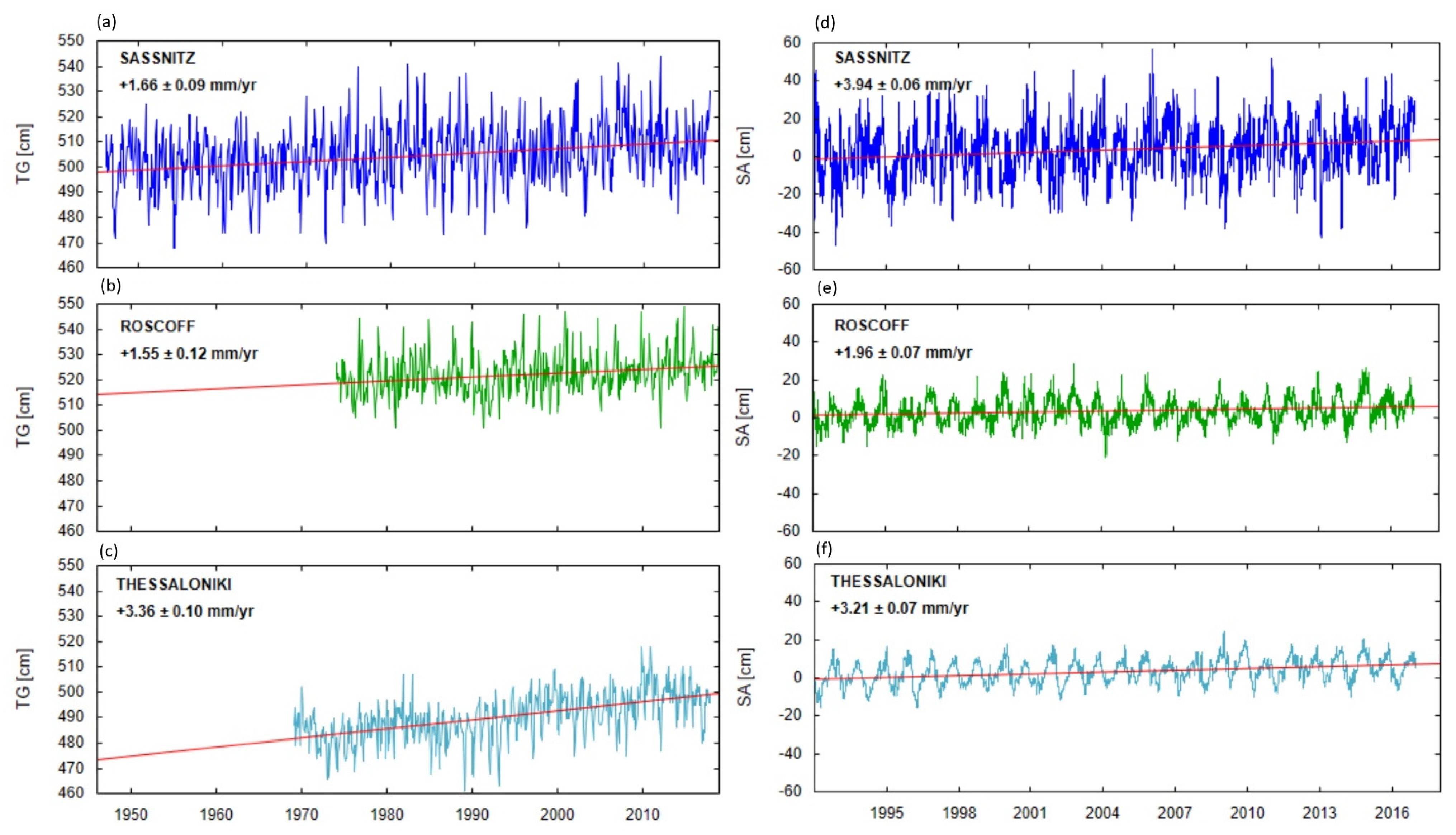
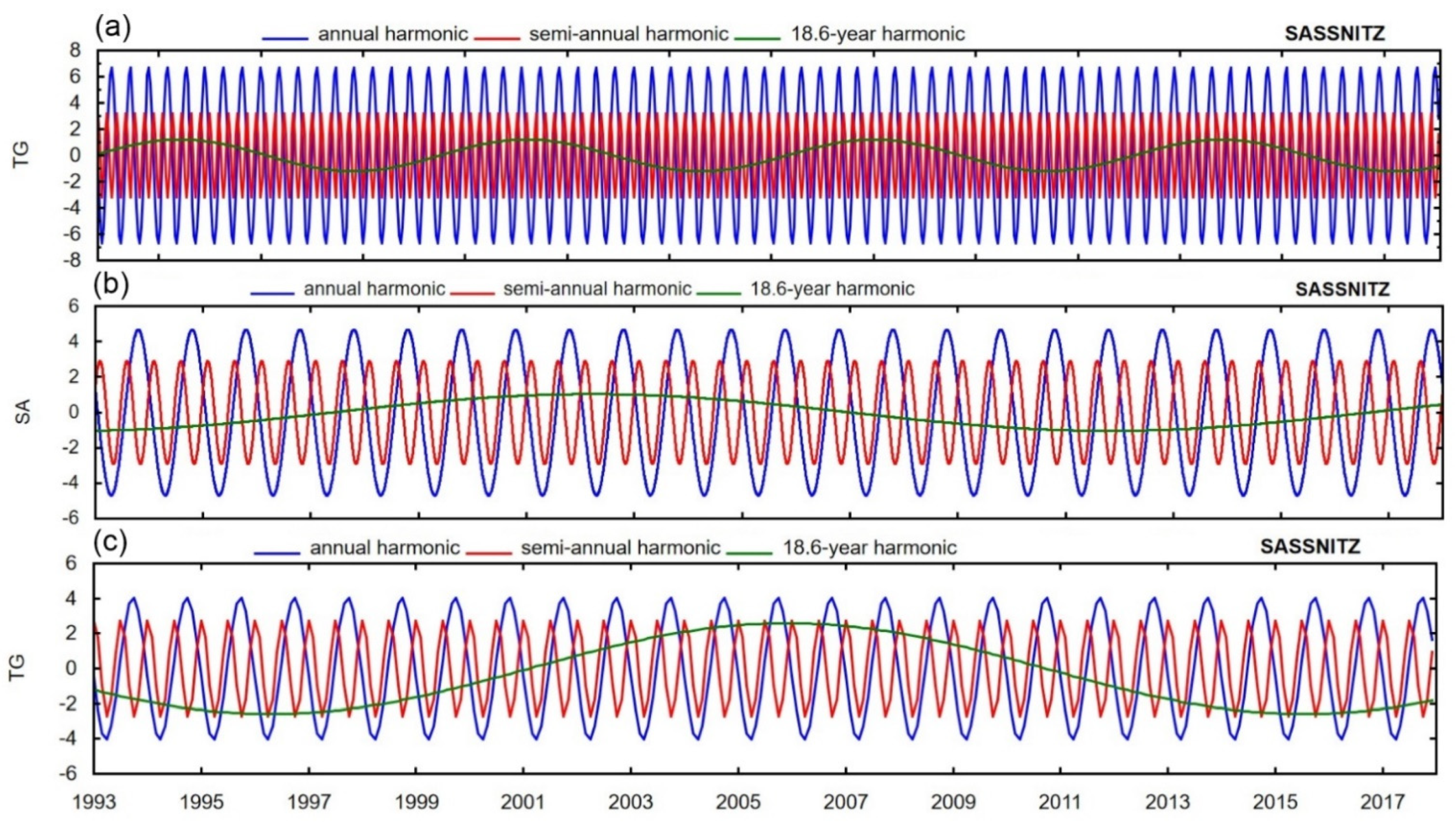
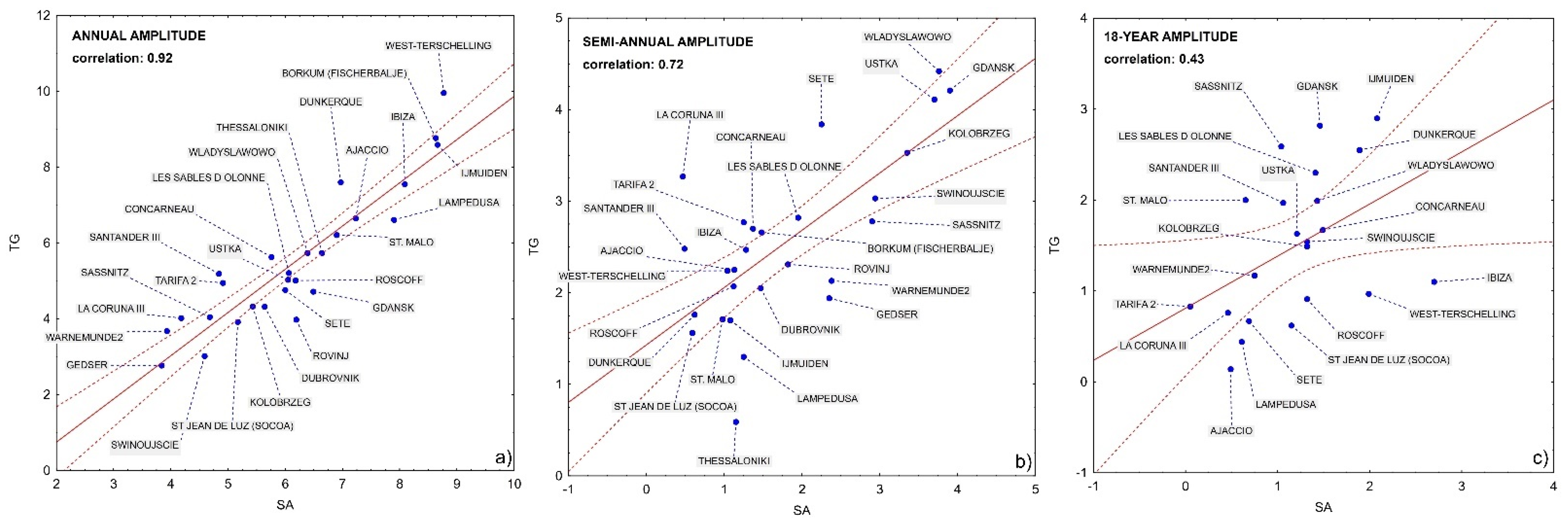
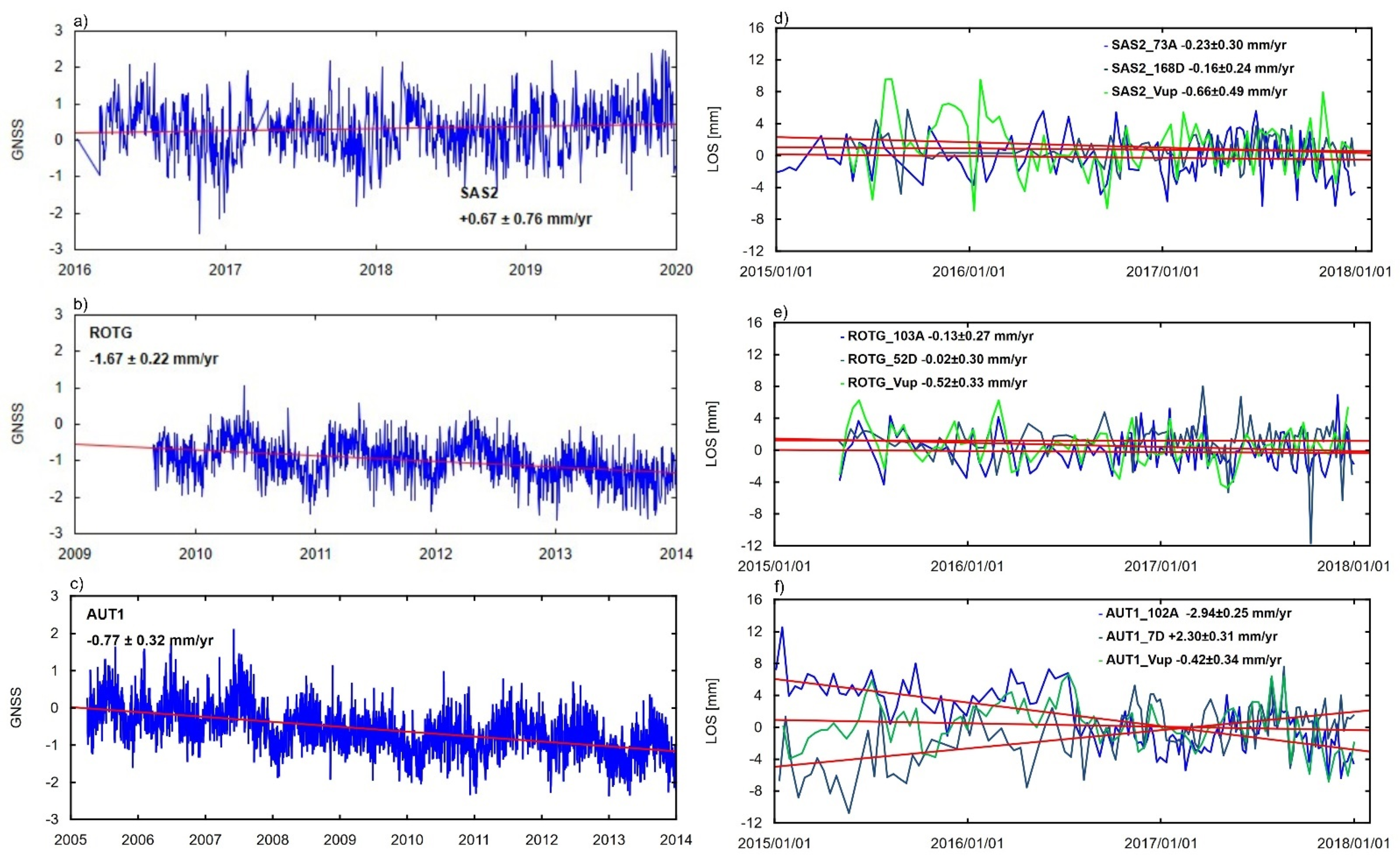
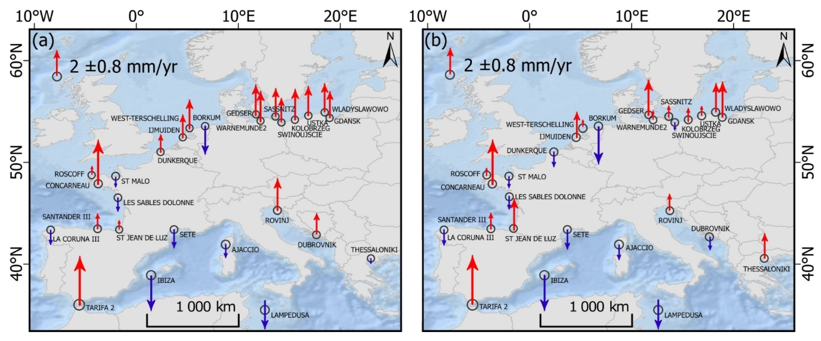
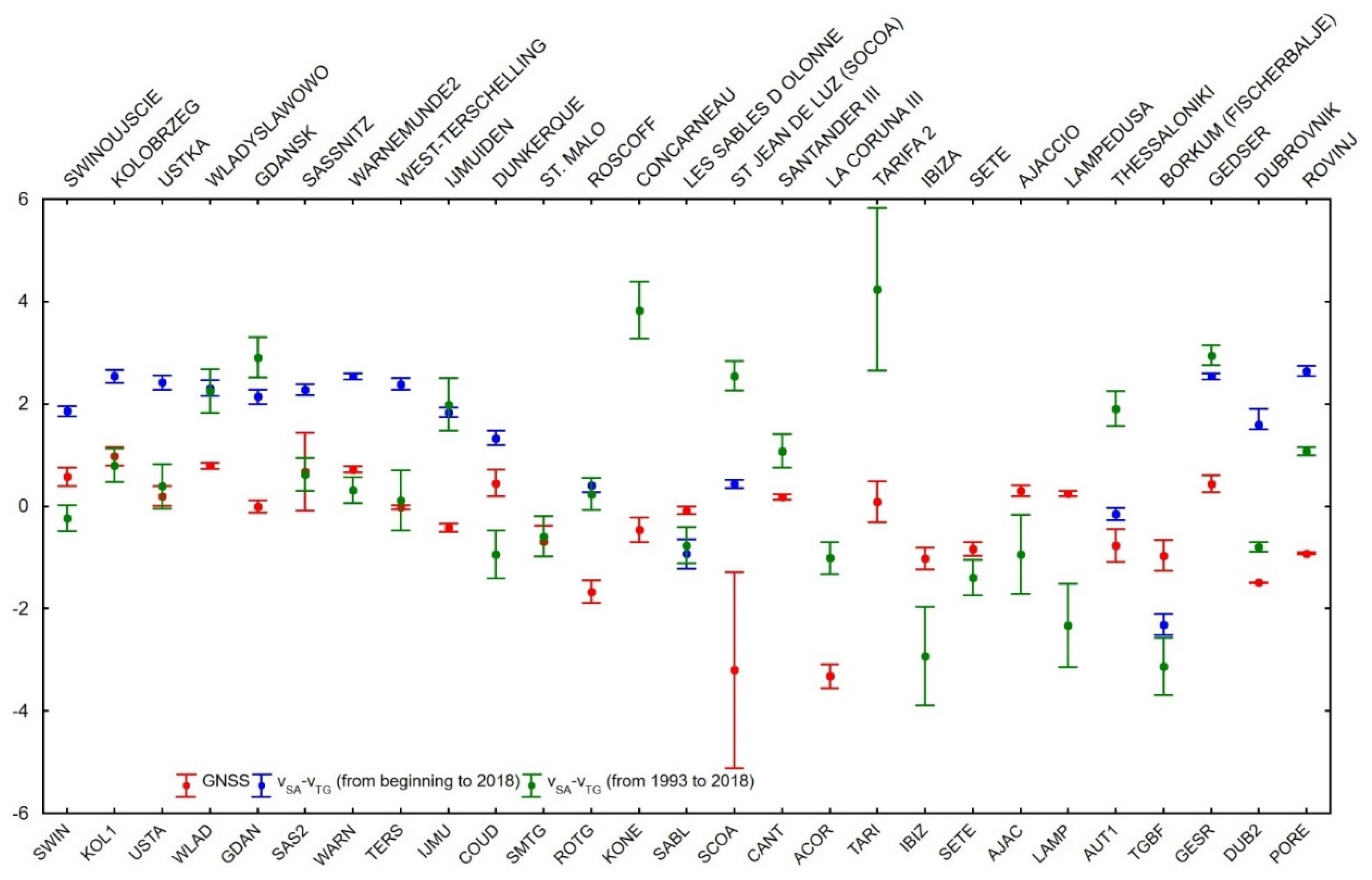
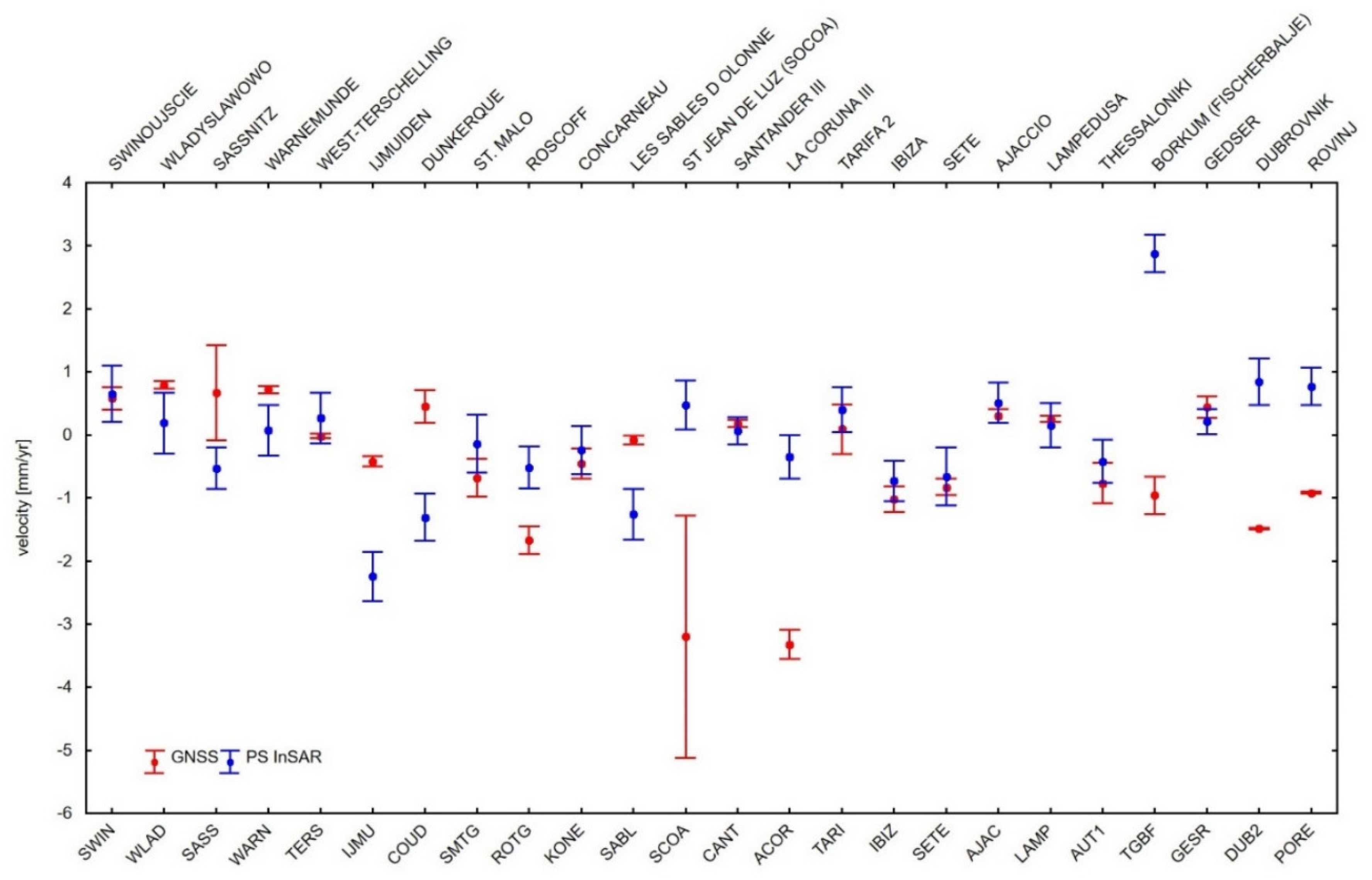
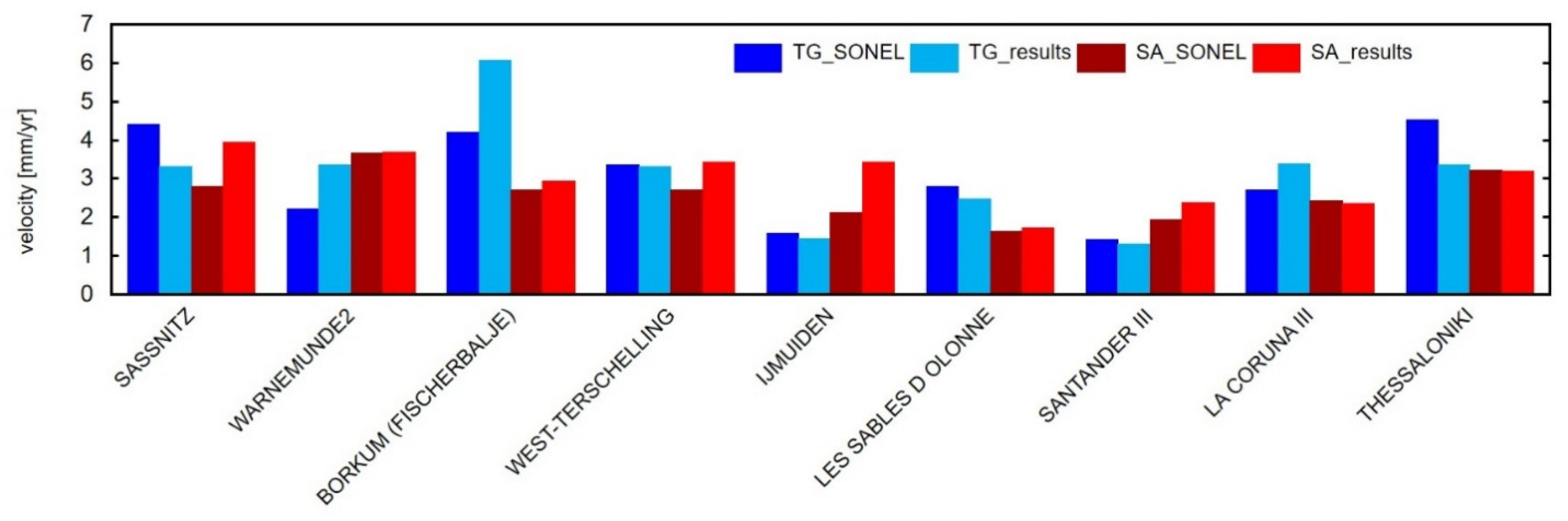
Then, the NNV was calculated, and the spatial interpolation was performed, taking into account the geostatistical properties of displacements in each measurement epoch. The PSI results were spatially interpolated by the Kriging method. PS point targets from ascending and descending tracks were interpolated separately. Based on a review of the literature [9,72], the ordinary Kriging method with a spherical, exponential and Gaussian semivariogram model were applied to the PSI vector data [61].

3. Results

Vertical crust movements in TG stations were estimated from different time series of TG data (Figure 12a) and SA data (Figure 12b) using robust linear regression [73]. Each difference in the time series of SA and coastal TG data was analysed by considering a linear trend and an annual, semiannual and 18.61-year cycle.

The results of the analysis were used to calculate linear trends in vertical crust movement on the TG sites along the European coast based on SA data minus TG data and at GNSS time series (GNSS stations closest to TG stations were considered). The velocity in coastal stations, estimated from the different time series of SA data minus TG data from the beginning of data to 2018, is shown in Figure 13a. The velocity in coastal stations, estimated from the different time series of SA data minus TG data from 1993–2018, is shown in Figure 13b.

In the TG dataset, trend changes in the European coastal zone ranged from −1.75 ± 1.59 mm/year (Tarifa2 station in Spain) to +5.26 ± 0.19 mm/year (Borkum station in Germany).

In the SA dataset, trend changes in the European coastal zone ranged from +0.87 ± 0.08 mm/year (Ibiza station in Spain) to +4.48 ± 0.08 mm/year (Gdansk station in Poland). The mean trend for all stations was determined at +2.92 ± 0.08 mm/year based on SA data in a different period (1993 to 2017). A comparison of both data sets revealed the highest trend values in the northern European coastal zone (Germany and Poland) and the lowest trend values in the southern European coastal zone (Spain).

The differences in the trend values calculated based on TG and SA data were greatest in the Tarifa2 station (+4.24 ± 1.59 mm/year) and smallest in the Roscoff station (+0.44 ± 0.08 mm/year).

Velocities in GNSS stations ranged from nearly 0 mm/year (TERS, SABL, CANT, TARI) to −3 mm/year (ACOR, SCOA). The trend standard error ranged from nearly 0 mm/year (SASS, WARN, TERS, SABL, CANT, LAMP) to ±2.0 mm/year (SCOA).

Vertical crust movement values were estimated based on multitime SAR data series, and they ranged from −2.24 ± 0.39 mm/year (IJMU) to +2.88 ± 0.30 mm/year (TGBF). The mean minimum standard error was ±0.20 mm/year (GESR), and the maximum standard error was ± 0.49 mm/year (SAS2). The greatest changes in velocity were observed in the coastal zone of Northwestern Europe. The mean velocity values in the stations in France, Belgium, the Netherlands and Germany were negative in the range of −2.24 ± 0.39 mm/year (IJMU) to −0.14 ± 0.46 mm/year (SMTG). The highest positive values were noted in TGBF (Germany) at +2.88 ± 0.30 mm/year and TERS (Netherlands) at +0.27 ± 0.40 mm/year. The stations in the Baltic Sea zone in Northern Europe moved with mean positive velocities: +0.65 ± 0.45 mm/year in SWIN, +0.19 ± 0.48 mm/year in WLAD, +0.21 ± 0.20 mm/year in GESR and +0.07 ± 0.40 mm/year in WARN. Stations on Rügen island in Germany moved with mean negative velocities: +0.66 ± 0.49 mm/year in SAS2 and +0.53 ± 0.33 mm/year in SASS. The stations in Southern Europe (Spain) were characterised by positive velocities in the range of +0.06 ± 0.22 mm/year (CANT) to +0.47 ± 0.39 mm/year (SCOA). Negative velocity was observed only in the ACOR station (−0.35 ± 0.35 mm/year). A map of vertical crust movements in coastal stations estimated from different time series of GNSS and PSInSAR data is presented in Figure 14.

The estimates of vertical crust movements obtained from GNSS stations and the combination of SA data minus TG data were compared in 27 sites along the European coast where both types of measurements were available.

The movement of the Earth’s crust determined from the combination of TG and SA data ranged from −2.31 ± 0.21 mm/year (Borkum, Fischerbalje) to + 2.54 ± 0.06 mm/year (Kolobrzeg, Gedser). The mean standard error was ±0.13 mm/year (TG data from the beginning of data to 2018) and ±0.47 mm/year (TG data for 1993–2017). The greatest standard error values were noted in Les Sables D’Olonne (±0.29 mm/year—TG to 2018) and TARIFA 2 (±1.59 mm/year—TG since 1993) (Figure 15).

The greatest differences in vertical movement calculated based on PSI data and GNSS data were noted in TGBF, SCOA, COUD, SAS2 and SASS stations. Differences were also observed in ACOR, IJMU, SABL and TERS stations. The vertical component of interpolated PS points was calculated according to Equation (7). The values obtained in GNSS stations and interpolated PS points are shown in Figure 16.

4. Discussion

The obtained results present vertical deformations in the proximity of selected GNSS stations located on the European coast along with an assessment of the actual accuracy.

Differences were observed in the rate of changes in average sea level determined based on TG data (long-term observations) along the European coast. The greatest changes were observed in tide gauges in the Mediterranean area. The rate of changes in the mean sea level increased to the south (positive values), and a decrease was observed in only two tide gauge stations (Tarifa2 station in Spain and Concarneau station in France).

The mean changes in sea level along the European coast, determined based on satellite altimetry data, increased towards the north. All changes in sea level were positive.

To validate the presented calculations, the velocity determined on selected stations were compared with SONEL measurements based on TG data. Based on TG data and SA data for 1993–2011, 1993–2014 and 1993–2015 time periods, nine European coastal stations were chosen (Sassnitz, Warnemunde 2, Borkum (Fisherbalje), West-Terschelling, Ijmuiden, Les Sables D’Olonne, Santander III, La Coruna III and Thessaloniki stations). SONEL velocity measurements (mm/year) were based on SA (Aviso Global MSLA heights in delayed time) and TG (PSMSL demeaned TG time series) [74]. The results are shown in Figure 17.

The comparison produced relatively satisfactory results. The greatest difference between the values calculated in this study and those determined in the SONEL network based on the TG time series was noted in the Borkum station. This discrepancy could be attributed to differences in the analysed time periods (1993–2011 in the SONEL network, 1993–2017 in this study).

Differences were observed in the vertical movements of the Earth’s crust determined from GNSS data (Figure 14a). The greatest negative vertical movements were observed in ACOR and SCOA stations. The greatest standard errors in velocity determination were noted in SAS2, ILDX and SCOA stations.

In real data time series, an accuracy of 0.1 mm per year can be achieved over a 100-year observation period. In time series without seasonal variations, an accuracy of 0.1 mm per year requires an observation period of 49 years [19]. To achieve an accuracy of 0.5 mm/year, a minimum observation period of 3 years is needed [20]. The above assumptions do not apply to AUT1, ILDX and SCOA stations. The calculated standard error values differ from the predicted values, which indicates that the time series is disrupted (the changes in coordinate values proceed in a disordered manner, and their cause is unknown). According to [13], the uncertainty of velocity determinations based on GNSS data ranges from 0.1 mm/year to 1.3 mm/year with a median of 0.21 mm/year. Both higher and lower accuracy values were obtained in this study. The velocity calculated in this study based on GNSS data differs from that calculated by the analytical centres in ULR, NGL and JPL (

Table 1. Velocities of crust movement calculated in this study are based on GNSS data and SONEL network data calculated by three analytical centres (ULR, NGL, JPL).

Analysis Centre	Time Span [Year]	ULR	NGL	JPL	In Work
Reference Frame, Ellipsoid		ITRF08, GRS80	ITRF14, GRS80	ITRF14, GRS80	ITRF08, GRS80
Reference Epoch		2004.4973	2012.386	2020.0001	2004.4973
GNSS STATION		Velocity ± Standard Error [mm/Year]	Velocity ± Standard Error [mm/Year]	Velocity ± Standard Error [mm/Year]	Velocity ± Standard Error [mm/Year]
SASS	11	0.83 ± 0.55	0.65 ± 0.64	0.63 ± 0.39	0.60 ± 0.06
SAS2	2	-	0.62 ± 1.56	-	0.67 ± 0.76
WARN	11	0.66 ± 0.59	0.22 ± 0.65	0.34 ± 0.36	0.72 ± 0.06
TERS	17	−0.18 ± 0.22	−0.63 ± 0.42	-	−0.02 ± 0.04
IJMU	9	−0.51 ± 0.34	−1.33 ± 0.57	-	−0.42 ± 0.08
COUD	6	−0.18 ± 0.65	−0.92 ± 0.58	-	0.45 ± 0.26
SMTG	4	−0.63 ± 0.47	−1.78 ± 0.59	-	−0.68 ± 0.30
ROTG	4	−1.28 ± 0.33	−1.92 ± 0.55	-	−1.67 ± 0.22
KONE	6	−0.46 ± 0.32	−0.78 ± 0.48	-	−0.46 ± 0.24
SABL	11	−0.05 ± 0.24	−0.46 ± 0.58	-	−0.08 ± 0.07
ILDX	7	Not robust	−1.21 ± 0.63	−0.96 ± 0.40	−1.52 ± 0.52
SCOA	8	−2.69 ± 0.28	−1.63 ± 0.59	−3.06 ± 0.46	−3.20 ± 1.92
CANT	13	0.03 ± 0.17	−0.70 ± 0.48	−0.78 ± 0.58	0.18 ± 0.05
ACOR	13	−2.20 ± 0.54	−2.49 ± 0.40	−2.21 ± 0.22	−3.32 ± 0.23
TARI	4	0.20 ± 0.59	2.09 ± 1.05	-	0.09 ± 0.40
IBIZ	9	−2.36 ± 0.18	−1.39 ± 0.51	-	−1.02 ± 0.21
SETE	6	−0.85 ± 0.27	−1.25 ± 0.56	-	−0.83 ± 0.13
AJAC	13	0.40 ± 0.14	0.56 ± 0.46	−0.04 ± 0.38	0.30 ± 0.11
LAMP	14	0.35 ± 0.28	−0.22 ± 0.48	−0.19 ± 0.41	0.25 ± 0.05
AUT1	8	−1.20 ± 0.31	−1.92 ± 0.50	-	−0.77 ± 0.32
TGBF	4	−0.75 ± 0.79	−0.52 ± 0.64	-	−0.96 ± 0.30
GESR	10	0.63 ± 0.66	0.22 ± 0.58	0.63 ± 0.39	0.44 ± 0.17
DUB2	8	-	−1.94 ± 0.89	-	−1.49 ± 0.01
PORE	9	-	1.51 ± 1.03	−1.03 ± 0.70	−0.92 ± 0.02

). The greatest differences were noted in IJMU, COUD, SMTG, SCOA, TARI, IBIZ and AUT1. Considerable differences were also observed in standard error values. These discrepancies indicate that the method of calculating and interpreting vertical shifts in time series (jumps) has a significant impact on the final result.

The results obtained during our research of vertical movement velocity on the coasts of Poland, Denmark and Germany was verified on the basis of the article [75]. Differences in values may be connected with the different length of the time series and chosen time periods.

The trends in mean sea level were determined by [76] based on TG data for the coastal areas in France (Dunkerque, Roscoff, Saint-Malo, Concarneau, Les Sables D’Olonne, Saint Jean De Luz, Sete and other locations that were not analysed in this study). Relative sea level trends and vertical land movements were determined for 1993–2018. The vertical land movements estimated in the cited study are consistent with the presented findings for the Saint-Malo station (−0.63 ± 0.55 mm/year in the cited study; −0.68 ± 0.30 mm/year in this study), Concarneau station (−0.46 ± 0.42 mm/year and −0.46 ± 0.24 mm/year, respectively), Les Sables D’Olonne station (−0.05 ± 0.37 mm/year and −0.08 ± 0.07 mm/year, respectively), Sete station (−0.87 ± 0.43 mm/year and −0.83 ± 0.13 mm/year, respectively) and Roscoff station (−1.28 ± 0.43 mm/year and −1.67 ± 0.26 mm/year, respectively). Differences were observed only in the Dunkerque station (−0.18 ± 0.71 in the cited study, +0.45 ± 0.26 mm/year in this study).

The values of crust movement determined with the use of Equation (1) are shown in Figure 13a,b. Crust movements were well above zero in 12 tide gauges (based on data for 1993–2017). Tide gauges were below zero in Lampedusa and Sassnitz, which could be attributed to a greater decrease in average water levels calculated based on TG data rather than SA data. According to [13], the uncertainty of velocity determinations based on GNSS data is three to four times lower on average in comparison with combined satellite radar altimetry minus TG data which ranges from 0.3 mm/year to 3.0 mm/year, with a median of 0.80 mm/year. The uncertainty of trends for time series of daily SA data ranges from 0.04 mm/year to 0.09 mm/year, and it is higher when monthly data are used (around 0.40 mm/year). The uncertainty of trends based on the entire TG time series (monthly data) ranges from 0.03 mm/year (time series covering approximately 200 years) to 1.59 mm/year (time series covering approximately 20 years).

The adopted method for verifying the velocity of GNSS stations was based on radar interferometry data generated with the use of the PSI approach. The results indicate that the velocities calculated in selected stations (TGBF, COUD, SCOA, TERS, SAS2 and SASS) based on SAR data differ in sign relative to the values calculated based on GNSS data. As shown in Figure 14a,b, the velocities calculated based on GNSS and SAR data differ in stations located on the North Sea and the Bay of Biscay. A considerable difference was observed in the SCOA station (−3.67 mm/year) where the standard error of velocity determination reached ±0.39 mm/year in the PSI method and ±1.92 mm/year in the calculations based on GNSS data. A large discrepancy was also noted in the ACOR station (−2.97 mm/year), where the standard error reached ±0.35 mm/year in the PSI approach and ±0.23 mm/year in the calculations based on GNSS data. In the TGBF station, the difference in the velocity was +3.84 mm/year with a standard error of ±0.30 mm/year in the PSI method and ±0.30 mm/year in the calculations based on GNSS data. On the other hand, the velocities calculated based on GNSS and SAR data are more similar in stations located on the Baltic Sea and the Mediterranean. The smallest difference was observed in the SWIN and LAMP stations. In the SWIN station, the difference in the velocity was +0.07 mm/year with a standard error of ±0.45 mm/year in the PSI method and ±0.18 mm/year in the calculations based on GNSS data. In the LAMP station, the difference in the velocity was −0.10 mm/year with a standard error of ±0.35 mm/year in the PSI approach and ±0.05 mm/year in the calculations based on GNSS data. The remaining velocity values resulted from the calculation of relative displacements in the PSI method as well as from differences in the analysed data sets and time periods.

5. Conclusions

TG and SA data were used to determine variations in sea level in the coastal zone. The results point to considerable differences in sea level trends, and they indicate that local and regional processes influence TG time series The results presented in the study point to land subsidence in the south and southwest along the European coast. These observations were confirmed by the data from permanent GNSS stations and InSAR systems. The InSAR technology helps with the determination of the vertical movements of the Earth’s crust (deformation) in the areas surrounding GNSS stations.

Different measurement techniques have different real accuracies in determining the vertical movements of the earth’s crust. The standard error from the combination of TG and SA data ranged from ±0.06 mm/year to ±0.21 mm/year at a long-time resolution and from ±0.31 mm/year to ±1.59 mm/year at a short-time resolution. The use of an unprecedented number of PSInSAR datasets allowed the estimation of a new level of accuracy in the range of ± 0.20 mm/year to ±0.49 mm/yy. The accuracy of the vertical movements of the Earth’s crust from GNSS data ranged from ±0.04 mm/year to ±1.92 mm/year. Comparing the PSInSAR results required the development of a new procedure: the workflow of determining the value of vertical movement velocities in GNSS stations based on InSAR data.

References

1. Billiris, H.; Paradissis, D.; Veis, G.; England, P.; Featherstone, W.; Parsons, B.; Cross, P.; Rands, P.; Rayson, M.; Sellers, P.; et al. Geodetic determination of tectonic deformation in central Greece from 1900 to 1988. Nature 1991, 350, 124–129. [Google Scholar] [CrossRef]
2. Blewitt, G.; Altamimi, Z.; Davis, J.; Gross, R.; Kuo, C.Y.; Lemoine, F.G.; Moore, A.W.; Neilan, R.E.; Plag, H.P.; Rothacher, M.; et al. Geodetic Observations and Global Reference Frame Contributions to Understanding Sea-Level Rise and Variability. Underst. Sea-Level Rise Var. 2010, 256–284. [Google Scholar] [CrossRef] [Green Version]
3. Douglas, B.C. Global sea level rise. J. Geophys. Res. 1991, 96, 6981. [Google Scholar] [CrossRef] [Green Version]
4. Hooper, A.; Segall, P.; Zebker, H. Persistent scatterer interferometric synthetic aperture radar for crustal deformation analysis, with application to Volcán Alcedo, Galápagos. J. Geophys. Res. Solid Earth 2007, 112, B07407. [Google Scholar] [CrossRef] [Green Version]
5. Zakarevičius, A. The results of investigations into vertical movements of the earth’s crust in ignalina nuclear power plant geodynamic polygon. Geod. Kartogr. 1997, 23, 78–85. [Google Scholar] [CrossRef]
6. Zhu, X.; Wang, R.; Sun, F.; Wang, J. A unified global reference frame of vertical crustal movements by satellite laser ranging. Sensors 2016, 16, 225. [Google Scholar] [CrossRef] [PubMed] [Green Version]
7. Cuffaro, M.; Carminati, E.; Doglioni, C. Horizontal versus vertical plate motions. eEarth Discuss. 2006, 1, 63–80. [Google Scholar] [CrossRef]
8. Bawden, G.W.; Thatcher, W.; Stein, R.S.; Hudnut, K.W.; Peltzer, G. Tectonic contraction across Los Angeles after removal of groundwater pumping effects. Nature 2001, 412, 812–815. [Google Scholar] [CrossRef]
9. Fuhrmann, T.; Caro Cuenca, M.; Knöpfler, A.; van Leijen, F.J.; Mayer, M.; Westerhaus, M.; Hanssen, R.F.; Heck, B. Estimation of small surface displacements in the Upper Rhine Graben area from a combined analysis of PS-InSAR, levelling and GNSS data. Geophys. J. Int. 2015, 203, 614–631. [Google Scholar] [CrossRef] [Green Version]
10. Nerem, R.S.; Mitchum, G.T. Estimates of vertical crustal motion derived from differences of TOPEX/POSEIDON and tide gauge sea level measurements. Geophys. Res. Lett. 2002, 29, 40-1–40-44. [Google Scholar] [CrossRef]
11. Soudarin, L.; Crétaux, J.F.; Cazenave, A. Vertical crustal motions from the DORIS space-geodesy system. Geophys. Res. Lett. 1999, 26, 1207–1210. [Google Scholar] [CrossRef]
12. Kowalczyk, K.; Rapiński, J. Evaluation of levelling data for use in vertical crustal movements model in Poland. Acta Geodyn. Geomater. 2013, 10, 1–10. [Google Scholar] [CrossRef] [Green Version]
13. Wöppelmann, G.; Marcos, M. Vertical land motion as a key to understanding sea level change and variability. Rev. Geophys. 2016, 54, 64–92. [Google Scholar] [CrossRef] [Green Version]
14. Kuo, C.Y.; Shum, C.K.; Braun, A.; Mitrovica, J.X. Vertical crustal motion determined by satellite altimetry and tide gauge data in Fennoscandia. Geophys. Res. Lett. 2004, 31, L01608. [Google Scholar] [CrossRef] [Green Version]
15. Fu, L.L.; Cazenave, A. Satellite altimetry and Earth sciences: A handbook of techniques and applications. Eos Trans. Am. Geophys. Union 2001, 82, 376. [Google Scholar] [CrossRef]
16. Cazenave, A.; Dominh, K.; Ponchaut, F.; Soudarin, L.; Cretaux, J.F.; Le Provost, C. Sea level changes from Topex-Poseidon altimetry and tide gauges, and vertical crustal motions from DORIS. Geophys. Res. Lett. 1999, 26, 2077–2080. [Google Scholar] [CrossRef]
17. García, D.; Vigo, I.; Chao, B.F.; Martínez, M.C. Vertical crustal motion along the Mediterranean and Black Sea coast derived from ocean altimetry and tide gauge Data. Pure Appl. Geophys. 2007, 164, 851–863. [Google Scholar] [CrossRef] [Green Version]
18. Vadivel, S.K.P.; Kim, D.J.; Jung, J.; Cho, Y.K.; Han, K.J. Monitoring the vertical land motion of tide gauges and its impact on relative sea level changes in Korean peninsula using sequential SBAS-InSAR time-series analysis. Remote Sens. 2021, 13, 18. [Google Scholar] [CrossRef]
19. Pajak, K.; Kowalczyk, K. A comparison of seasonal variations of sea level in the southern Baltic Sea from altimetry and tide gauge data. Adv. Sp. Res. 2019, 63, 1768–1780. [Google Scholar] [CrossRef]
20. Ihde, J.; Augath, W.; Sacher, M. The Vertical Reference System for Europe. In IAG SYMPOSIA; Springer: Berlin/Heidelberg, Germany, 2002; Volume 124, pp. 345–350. [Google Scholar]
21. Ferretti, A.; Prati, C.; Rocca, F. Permanent scatterers in SAR interferometry. IEEE Int. Geosci. Remote Sens. Symp. 1999, 39, 1528–1530. [Google Scholar] [CrossRef]
22. Wieczorek, B. Evaluation of deformations in the urban area of Olsztyn using Sentinel-1 SAR interferometry. Acta Geodyn. Geomater. 2020, 17, 5–18. [Google Scholar] [CrossRef] [Green Version]
23. Santamaría-Gómez, A.; Gravelle, M.; Wöppelmann, G. Long-term vertical land motion from double-differenced tide gauge and satellite altimetry data. J. Geod. 2014, 88, 207–222. [Google Scholar] [CrossRef]
24. Tretyak, K.R.; Dosyn, S.I. Analysis of the Results of Vertical Crust Movement Velocities of the European Coastline per the Tide Gauge and GNSS-Observation Data|Academic Journals and Conferences. Available online: http://science.lpnu.ua/jgd/all-volumes-and-issues/221-2016/analysis-results-vertical-crust-movement-velocities-european (accessed on 13 February 2020).
25. Bitharis, S.; Ampatzidis, D.; Pikridas, C.; Fotiou, A.; Rossikopoulos, D.; Schuh, H. The Role of GNSS Vertical Velocities to Correct Estimates of Sea Level Rise from Tide Gauge Measurements in Greece. Mar. Geod. 2017, 40, 297–314. [Google Scholar] [CrossRef]
26. Grgić, M.; Nerem, R.S.; Bašić, T. Absolute Sea Level Surface Modeling for the Mediterranean from Satellite Altimeter and Tide Gauge Measurements. Mar. Geod. 2017, 40, 239–258. [Google Scholar] [CrossRef]
27. Kowalczyk, K.; Pajak, K.; Naumowicz, B. Modern vertical crustal movements of the southern baltic coast from tide gauge, satellite altimetry and GNSS observations. Acta Geodyn. Geomater. 2019, 16, 242–252. [Google Scholar] [CrossRef]
28. Dheenathayalan, P.; Hanssen, R. Target characterization and interpretation of deformation using persistent scatterer interferometry and polarimetry. In Proceedings of the 5th International Workshop on Science and Applications of SAR Polarimetry and Polarimetric Interferometry, PolinSAR 2011, Frascati, Italy, 24–28 January 2011; Volume 695, p. 8. [Google Scholar]
29. Walters, R.J.; Parsons, B.; Wright, T.J. Constraining crustal velocity fields with InSAR for Eastern Turkey: Limits to the block-like behavior of Eastern Anatolia. J. Geophys. Res. Solid Earth 2014, 119, 5215–5234. [Google Scholar] [CrossRef]
30. Borghi, A.; Cannizzaro, L.; Vitti, A. Advanced techniques for discontinuity detection in GNSS coordinate time-series. an Italian case study. In Proceedings of the Geodesy for Planet Earth: 2009 IAG Symposium, Buenos Aires, Argentina, 31 August 31–4 September 2009; Springer: Berlin/Heidelberg, Germany, 2012; Volume 136, pp. 627–634. [Google Scholar]
31. Gazeaux, J.; Williams, S.; King, M.; Bos, M.; Dach, R.; Deo, M.; Moore, A.W.; Ostini, L.; Petrie, E.; Roggero, M.; et al. Detecting offsets in GPS time series: First results from the detection of offsets in GPS experiment. J. Geophys. Res. Solid Earth 2013, 118, 2397–2407. [Google Scholar] [CrossRef] [Green Version]
32. Kowalczyk, K.; Rapinski, J. Verification of a GNSS time series discontinuity detection approach in support of the estimation of vertical crustal movements. ISPRS Int. J. Geo-Inf. 2018, 7, 149. [Google Scholar] [CrossRef] [Green Version]
33. Perfetti, N. Detection of station coordinate discontinuities within the Italian GPS Fiducial Network. J. Geod. 2006, 80, 381–396. [Google Scholar] [CrossRef]
34. Tretyak, K.; Dosyn, S. Study of Vertical Movements of the European Crust Using Tide Gauge and Gnss Observations. Rep. Geod. Geoinform. 2015, 97, 112–131. [Google Scholar] [CrossRef] [Green Version]
35. Völksen, C.; Wassermann, J. Recent Crustal Deformation and Seismicity in Southern Bavaria revealed by GNSS observations. In Proceedings of the Symposium EUREF, Budapest, Hungary, 29–31 May 2013. [Google Scholar]
36. Borkowski, A.; Bosy, J.; Kontny, B. Time series analysis of EPN stations as a criterion of choice of reference stations for local geodynamic networks. Artif. Satell. 2003, 38, 15–28. [Google Scholar]
37. Grubbs, F.E. Procedures for Detecting Outlying Observations in Samples. Technometrics 1969, 11, 1–21. [Google Scholar] [CrossRef]
38. Stefansky, W. Rejecting Outliers in Factorial Designs. Technometrics 1972, 14, 469–479. [Google Scholar] [CrossRef]
39. Trauth, M.H.; Trauth, M.H. Statistics on Directional Data. In MATLAB® Recipes for Earth Sciences; Springer: Berlin/Heidelberg, Germany, 2010; pp. 311–326. [Google Scholar]
40. Klos, A.; Bogusz, J.; Figurski, M.; Kosek, W. On the handling of outliers in the GNSS time series by means of the noise and probability analysis. In Proceedings of the IAG Scientific Assembly, Postdam, Germany, 1–6 September 2013; Springer: Berlin/Heidelberg, Germany, 2015; Volume 143, pp. 657–664. [Google Scholar]
41. Williams, S.D.P. The effect of coloured noise on the uncertainties of rates estimated from geodetic time series. J. Geod. 2003, 76, 483–494. [Google Scholar] [CrossRef]
42. Bogusz, J.; Klos, A. On the significance of periodic signals in noise analysis of GPS station coordinates time series. GPS Solut. 2016, 20, 655–664. [Google Scholar] [CrossRef] [Green Version]
43. Dong, D.; Fang, P.; Bock, Y.; Cheng, M.K.; Miyazaki, S. Anatomy of apparent seasonal variations from GPS-derived site position time series. J. Geophys. Res. Solid Earth 2002, 107, ETG 9-1–ETG 9-16. [Google Scholar] [CrossRef] [Green Version]
44. Jevrejeva, S.; Grinsted, A.; Moore, J.C.; Holgate, S. Nonlinear trends and multiyear cycles in sea level records. J. Geophys. Res. 2006, 111, C09012. [Google Scholar] [CrossRef] [Green Version]
45. Wiśniewski, B.; Wolski, T.; Musielak, S. A long-term trend and temporal fluctuations of the sea level at the Polish Baltic coast. Oceanol. Hydrobiol. Stud. 2011, 40, 96–107. [Google Scholar] [CrossRef]
46. Pollock, D.S.G. Statistical Fourier Analysis: Clarifications and Interpretations. J. Time Ser. Econom. 2008, 1, 1–47. [Google Scholar] [CrossRef] [Green Version]
47. Haigh, I.D.; Eliot, M.; Pattiaratchi, C. Global influences of the 18.61 year nodal cycle and 8.85 year cycle of lunar perigee on high tidal levels. J. Geophys. Res. Ocean. 2011, 116, C06025. [Google Scholar] [CrossRef] [Green Version]
48. Holgate, S.J.; Matthews, A.; Woodworth, P.L.; Rickards, L.J.; Tamisiea, M.E.; Bradshaw, E.; Foden, P.R.; Gordon, K.M.; Jevrejeva, S.; Pugh, J. New Data Systems and Products at the Permanent Service for Mean Sea Level. J. Coast. Res. 2012, 29, 493. [Google Scholar] [CrossRef]
49. PSMSL. Available online: https://www.psmsl.org/ (accessed on 12 December 2019).
50. AVISO. Available online: http://www.aviso.oceanobs.com (accessed on 15 May 2019).
51. CMEMS. Available online: http://marine.copernicus.eu/services-portfolio/access-to-products/ (accessed on 15 May 2019).
52. Kakkuri, J. Character of the Fennoscandian land uplift in the 20th century. Geol. Surv. Finl. 1987, 2, 15–20. [Google Scholar]
53. Bogusz, J.; Kłos, A.; Grzempowski, P.; Kontny, B. Modelling the Velocity Field in a Regular Grid in the Area of Poland on the Basis of the Velocities of European Permanent Stations. Pure Appl. Geophys. 2014, 171, 809–833. [Google Scholar] [CrossRef] [Green Version]
54. Jin, S.; Park, P.H.; Zhu, W. Micro-plate tectonics and kinematics in Northeast Asia inferred from a dense set of GPS observations. Earth Planet. Sci. Lett. 2007, 257, 486–496. [Google Scholar] [CrossRef]
55. NGL. Available online: http://geodesy.unr.edu/ (accessed on 12 December 2019).
56. Goldstein, R.M.; Zebker, H.A.; Werner, C.L. Satellite radar interferometry: Two-dimensional phase unwrapping. Radio Sci. 1988, 23, 713–720. [Google Scholar] [CrossRef] [Green Version]
57. Monti-Guarnieri, A.; Parizzi, F.; Pasquali, P.; Prati, C.; Rocca, F. SAR interferometry experiments with ERS-1. In Proceedings of the International Geoscience and Remote Sensing Symposium (IGARSS), Tokyo, Japan, 18–21 August 1993; Volume 3, pp. 991–993. [Google Scholar]
58. Zebker, H.A.; Villasenor, J. Decorrelation in interferometric radar echoes. IEEE Trans. Geosci. Remote Sens. 1992, 30, 950–959. [Google Scholar] [CrossRef] [Green Version]
59. Berardino, P.; Fornaro, G.; Lanari, R.; Sansosti, E. A new algorithm for surface deformation monitoring based on small baseline differential SAR interferograms. IEEE Trans. Geosci. Remote Sens. 2002, 40, 2375–2383. [Google Scholar] [CrossRef] [Green Version]
60. Hooper, A.; Zebker, H.; Segall, P.; Kampes, B. A new method for measuring deformation on volcanoes and other natural terrains using InSAR persistent scatterers. Geophys. Res. Lett. 2004, 31, 1–5. [Google Scholar] [CrossRef]
61. Foumelis, M. Vector-based approach for combining ascending and descending persistent scatterers interferometric point measurements. Geocarto Int. 2016, 33, 38–52. [Google Scholar] [CrossRef]
62. Fuhrmann, T.; Garthwaite, M.; Lawrie, S.; Brown, N. Combination of GNSS and InSAR for Future Australian Datums. In Proceedings of the International Global Navigation Satellite Systems Association IGNSS Symposium 2018, Sydney, Australia, 7–9 February 2018; pp. 2–9. [Google Scholar]
63. Fuhrmann, T.; Garthwaite, M.C. Resolving Three-Dimensional Surface Motion with InSAR: Constraints from Multi-Geometry Data Fusion. Remote Sens. 2019, 11, 241. [Google Scholar] [CrossRef] [Green Version]
64. Isya, N.H.; Niemeier, W.; Gerke, M. 3D Estimation of slow ground motion using insar and the slope aspect assumption, a case study: The puncak pass landslide, Indonesia. ISPRS Ann. Photogramm. Remote Sens. Spat. Inf. Sci. 2019, 4, 623–630. [Google Scholar] [CrossRef] [Green Version]
65. Hu, J.; Li, Z.W.; Ding, X.L.; Zhu, J.J.; Zhang, L.; Sun, Q. Resolving three-dimensional surface displacements from InSAR measurements: A review. Earth-Sci. Rev. 2014, 133, 1–17. [Google Scholar] [CrossRef]
66. Meyer, F.J. Topography and displacement of polar glaciers from multi-temporal SAR interferograms. Polar Rec. 2007, 43, 331–343. [Google Scholar] [CrossRef]
67. Joughin, L.R.; Kwok, R.; Fahnestock, M.A. Interferometric estimation of three-dimensional ice-flow using ascending and descending passes. IEEE Trans. Geosci. Remote Sens. 1998, 36, 25–37. [Google Scholar] [CrossRef] [Green Version]
68. Graniczny, M.; Čyžienė, J.; Van Leijen, F.; Minkevičius, V.; Mikulėnas, V.; Satkūnas, J.; Przyłucka, M.; Kowalski, Z.; Uścinowicz, S.; Jegliński, W.; et al. Vertical ground movements in the polish and lithuanian baltic coastal area as measured by satellite interferometry. Baltica 2015, 28, 65–80. [Google Scholar] [CrossRef]
69. Samieie-esfahany, S.; Hanssen Ramon, F.; Van Thienen-visser, K.; Muntendam-Bos, A. On the effect of horizontal deformation on InSAR subsidence estimates. In Proceedings of the ‘Fringe 2009 Workshop’, Frascati, Italy, 30 November–4 December 2009; pp. 1–7. [Google Scholar]
70. Bakon, M.; Oliveira, I.; Perissin, D.; Sousa, J.; Papco, J. A data mining approach for multivariate outlier detection in heterogeneous 2D point clouds: An application to post-processing of multi-temporal InSAR results. In Proceedings of the International Geoscience and Remote Sensing Symposium (IGARSS), Beijing, China, 10–15 July 2016; Institute of Electrical and Electronics Engineers Inc.: Manhattan, NY, USA, 2016; pp. 56–59. [Google Scholar]
71. Foumelis, M.; Chalkias, C.; Plank, S. Influence of Satellite Imaging Geometry on ASTER and SRTM Global Digital Elevation Models. In Proceedings of the 10th International Congress of the Hellenic Geographical Society, Thessaloniki, Greece, 22–24 October 2014; pp. 275–287. [Google Scholar]
72. Agudo, M.; Crosetto, M.; Raucoules, D.; Bourgine, B.; Closset, L.; Bremmer, C.; Veldkamp, H.; Tragheim, D.; Bateson, L. Defining the Methods for PSI Validation and Inter-Comparison. Raport BRGM/RP-55636-FR. 2006. Available online: https://earth.esa.int/psic4/PSIC4_Defining_Methods-PSI_Validation_and_Intercomparison_rprt_Task6.pdf (accessed on 12 February 2020).
73. Street, J.O.; Carroll, R.J.; Ruppert, D. A note on computing robust regression estimates via iteratively reweighted least squares. Am. Stat. 1988, 42, 152–154. [Google Scholar] [CrossRef] [Green Version]
74. SONEL Système d’Observation du Niveau des Eaux Littorales. Available online: https://www.sonel.org/ (accessed on 12 February 2020).
75. Bogusz, J.; Klos, A.; Pokonieczny, K. Optimal strategy of a GPS position time series analysis for post-glacial rebound investigation in Europe. Remote Sens. 2019, 11, 1209. [Google Scholar] [CrossRef] [Green Version]
76. Dodet, G.; Bertin, X.; Bouchette, F.; Gravelle, M.; Testut, L.; Wöppelmann, G. Characterization of Sea-level Variations Along the Metropolitan Coasts of France: Waves, Tides, Storm Surges and Long-term Changes. J. Coast. Res. 2019, 88, 10. [Google Scholar] [CrossRef]
Figure 1. The location of GNSS stations which were used to determine vertical crustal movements based on TG, SA and InSAR data.
Remotesensing 13 02173 g001
Figure 2. (ac) Time series of mean sea level anomalies based on TG data. (df) Time series of mean sea levels based on SA data. The time series are displayed with arbitrary offsets for presentation purposes. The units are in centimetres.
Remotesensing 13 02173 g002
Figure 3. (a) Annual, semiannual and 18.61-year harmonics functions based on TG data for 1946–2017. (b) Annual, semiannual and 18.61-year harmonics functions based on SA data for 1993–2017. (c) Annual, semiannual and 18.61-year harmonics functions based on TG data for 1993–2017 in the Sassnitz station. The units are in centimetres.
Remotesensing 13 02173 g003
Figure 4. (a) Annual, (b) semiannual and (c) 18.61-year amplitudes of the seasonal cycle based on SA and TG time series. The correlation coefficients for amplitude were calculated based on SA and TG data (blue circles-dispersion plot; area marked by red dashed lines-95% confidence interval of the regression line). The amplitude units are centimetres.
Remotesensing 13 02173 g004
Figure 5. (ac) The time series of 3 selected GNSS stations from a total of 27 stations. (df) The units are in centimetres. The time series is in the line of sight (LOS) displacement (in mm) of two persistent scatterer points with an ascending and descending track within GNSS stations. The time series are displayed with arbitrary offsets for presentation purposes.
Remotesensing 13 02173 g005
Figure 6. Distance between GNSS stations and the nearest TG (the longest distance between a TG station and a GNSS station was 16.069 km, and the shortest distance between a TG station and a GNSS station was 0.002 km).
Remotesensing 13 02173 g006
Figure 7. Steps of the VSED algorithm (KONE station): (a) Left and right moving averages are calculated according to Equation (2) from [32]; (b) Left and right standard deviations are the square root of Equation (3) from [32]; (c) The output function is Equation (4) from [32]; (d) The result of detection. The units on the y-axis are in metres. The units on the x-axis are the number of observations.
Remotesensing 13 02173 g007
Figure 8. The influence of height determination error σH on the number of jumps in the analysed time series of coordinates from the GNSS station.
Remotesensing 13 02173 g008
Figure 9. (a) Sentinel-1 (LOS) mean deformation velocity maps for 2015–2017 in the Sassnitz station for ascending, (b) descending orbits. (c) In the Roscoff station for ascending, (d) and descending orbits. (e) In the Thessaloniki station for ascending, (f) and descending orbits. Coloured dots represent the location of a PS, and the displacement rate measured at each point is marked with an appropriate colour. Selected reference points (SASS, SAS2, ROTG, AUT1) are shown as green squares. World Imagery data constitute the background.
Remotesensing 13 02173 g009
Figure 10. Distances between selected PS points from ascending and descending tracks and the GNSS station. PS targets were ordered from the longest distance (334.28 m) from the WLAD station, and the shortest distance (0.98 m) from the IJMU station.
Remotesensing 13 02173 g010
Figure 11. Workflow scheme of determining the value of vertical movement velocities in GNSS stations based on InSAR data.
Remotesensing 13 02173 g011
Figure 12. (a) Map of the linear trend in coastal stations estimated from different time series of TG data (TG data from the beginning of data to 2018). (b) Map of the linear trend in coastal stations estimated from different time series of SA data (SA data from 1993 to 2017); the units on both pictures are in mm/year. The linear trend standard errors are visualized by black circles. Positive values of the linear trend are visualized by a red arrow. Negative values of the linear trend are visualized by a blue arrow.
Remotesensing 13 02173 g012
Figure 13. (a) Map of vertical crust movements in coastal stations estimated from different time series of SA data minus TG data (from the beginning of data to 2018). (b) Map of vertical crust movements in coastal stations estimated from different time series of SA data minus TG data (1993–2017); the units on both pictures are in mm/year. The linear trend standard errors are visualized by black circles. Positive values of the linear trend are visualized by a red arrow. Negative values of the linear trend are visualized by a blue arrow.
Remotesensing 13 02173 g013
Figure 14. (a) Map of vertical crust movement in coastal stations estimated from different time series of GNSS data. GNSS data were acquired from 27 GNSS stations which are colocated with or positioned in the proximity of a TG station on the European coast. (b) Map of vertical motion based on multitime SAR data series for 2015–2017; the units on both pictures are in mm/year. The linear trend standard errors are visualized by black circles. Positive values of the linear trend are visualized by a red arrow. Negative values of the linear trend are visualized by a blue arrow.
Remotesensing 13 02173 g014
Figure 15. Vertical crust movements in TG sites along the European coast based on SA and TG data and the corresponding GNSS.
Remotesensing 13 02173 g015
Figure 16. Vertical crust movements in TG sites along the European coast derived from PSInSAR data and the corresponding GNSS data.
Remotesensing 13 02173 g016
Figure 17. A comparison of the velocity estimated in nine European coastal zone stations and SONEL stations based on TG and SA time series.
Remotesensing 13 02173 g017