Abstract
Data collection from large areas of native forests poses a challenge. The present study aims at assessing the use of UAV for forest inventory on native forests in Southern Chile, and seeks to retrieve both stand and tree level attributes from forest canopy data. Data were collected from 14 plots (45 × 45 m) established at four locations representing unmanaged Chilean temperate forests: seven plots on secondary forests and seven plots on old-growth forests, including a total of 17 different native species. The imagery was captured using a fixed-wing airframe equipped with a regular RGB camera. We used the structure from motion and digital aerial photogrammetry techniques for data processing and combined machine learning methods based on boosted regression trees and mixed models. In total, 2136 trees were measured on the ground, from which 858 trees were visualized from the UAV imagery of the canopy, ranging from 26% to 88% of the measured trees in the field (mean = 45.7%, SD = 17.3), which represented between 70.6% and 96% of the total basal area of the plots (mean = 80.28%, SD = 7.7). Individual-tree diameter models based on remote sensing data were constructed with R2 = 0.85 and R2 = 0.66 based on BRT and mixed models, respectively. We found a strong relationship between canopy and ground data; however, we suggest that the best alternative was combining the use of both field-based and remotely sensed methods to achieve high accuracy estimations, particularly in complex structure forests (e.g., old-growth forests). Field inventories and UAV surveys provide accurate information at local scales and allow validation of large-scale applications of satellite imagery. Finally, in the future, increasing the accuracy of aerial surveys and monitoring is necessary to advance the development of local and regional allometric crown and DBH equations at the species level.
1. Introduction
Native forests cover a large percentage of land in South America [1], with vast areas of old-growth and secondary forests [2] which are playing an essential ecological role supporting biodiversity, as a carbon sink and as an important economic resource for local communities [3,4]. The essential roles of these forests underline the need for basic information concerning standing biomass, carbon stock, and biodiversity estimates, among others, and their change over space and time [5]. Traditionally, forest inventory has been the main tool for collecting quantitative data about the state of the forests, relying on the direct measurement of diameter at breast height (DBH) and tree height, which are the basis for, for example, biomass estimates or carbon storage via allometric equations using the relationships between tree attributes and endogenous and exogenous variability [6,7].
In native forests, however, this information is often scarce; the lack of a direct industrial use, the land tenancy, or the absence of a national forest inventory in the countries of the area [8,9] translates into limitations in data available for an effective quantification of forest resources based on ground samples. In addition, large and often remote areas covered by native forests pose an additional important challenge [10].
The use of aerial inventory as an alternative to ground measurements represents an opportunity, given that it is enhanced by recent computational advances [11]. Remote measurement of tree crowns reduces the uncertainty associated with larger area estimates, providing continuous data of forests presenting high structural and compositional variability [12,13]. The use of airborne laser scanning (ALS) has meant a significant technological improvement for assessing forest attributes [14]; however, its use in South America has been only moderate, mainly restricted to forestlands with high economic value.
On the other hand, digital aerial photogrammetry (DAP) is a valid alternative for local level estimates when spatially continuous data are needed [11,15,16,17]. The use of DAP combined with unmanned aerial vehicles (UAV) and structure from motion (SfM) algorithms can generate high-quality aerial datasets of forest [18] for specific areas, that suppose a low investment alternative when ALS data are not available. A regular RGB camera mounted on a UAV offers different opportunities for data retrieval, i.e., high-resolution and georeferenced RGB orthomosaics, photogrammetric point clouds, and high-resolution surface elevation models [19]. Red, green, and blue (RGB) mosaics and digital surface models can have a spatial resolution close to 1 cm, depending on flight altitude and sensor type [20], using structure from motion (SfM) algorithms that estimate three-dimensional (3D) camera poses and scene points from uncalibrated images, creating the basis for 3D surface models from the point cloud data [19,21].
In these conditions, the use of SfM algorithms has become a promising cost-effective tool to use for operational and forestry research [14] and, more specifically, for forest monitoring [10,22], gap detection [9,23,24], individual-tree detection [25], forest recovery [26,27], canopy structure [28,29] and other related applications for forest inventories [30,31,32,33,34], which makes it a valid approach that can retrieve objective focused parameters and adapt to the extent of a study area, the season, or the spatial resolution needed, among others [35,36,37].
Despite the growing number of applications for these approaches, there are few studies in South America assessing their use in complex native forests. The present study aims at evaluating the use of a UAV for forest assessment on temperate forests in Southern Chile, aiming to retrieve a stand’s density, basal area (BA), and biodiversity indicators, as well as structure and forest canopy variables.
2. Materials and Methods
2.1. Study Sites
The analyses were performed at four locations, selected to represent unmanaged Chilean temperate forests (Figure 1). In total, 14 plots (45 × 45 m) were established, seven plots on secondary forests and seven plots on old-growth forests. Three of the plots were located at the protected national reserve Malalcahuello (38°24′S, 71°36′W) in Araucaria araucana and Nothofagus dombeyi stands (Table 1, see plots a, b, and c), two plots were located at the Parque Ecológico y Cultural Rucamanque (38°39′S, 72°35′W), in mixed forests of Aextoxicon punctatum, N. obliqua, and Eucryphia cordifolia (plot e), one plot was located in a secondary forest of N. obliqua (plot w), two plots on private forest lands located at Flor del Lago (39°12′S, 72°11′W) in old-growth forests dominated by A. punctatum, Persea lingue, and E. cordifolia (Table 1, plots f and g), three plots at a secondary forest dominated by N. obliqua, P. lingue, and A. punctatum (plots x, y, and z), and finally, two plots were established at Pucón (39°17′S, 71°53′W), in an old-growth forest dominated by N. dombeyi, which included P. lingue and A. punctatum (plot d), and in a young stand dominated by N. obliqua which included P. lingue and Gevuina avellana (plots t, u, and v). All the plots were established on flat areas (slope below 5%). At each plot, all trees with a DBH over 5 cm were identified and measured, and their location (using local coordinates), DBH, height, and crown diameter were recorded, the latter by measuring the larger diameter and its perpendicular one. The location of each tree was performed relative to the plot center, by bearing-and-distance, using a distance tape and a compass.
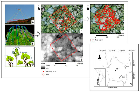
Figure 1.
Location of the sites and illustration of the steps performed in the acquisition and processing of the data. (A) Image acquisition; (B) structure from motion (SfM); (C) illustration of SfM estimation of the digital surface model (DSM); (D) position of every individual-tree DBH over 5 cm, over the high-resolution mosaic of the stand; (E) DSM of the stand; (F) association of each tree crown with its field measurements; (G) the study site.

Table 1.
Stand variables, dominant species, and structure of the plots (ground data). QMD, observed quadratic mean diameter. The mean and standard deviation of crow area and volume were calculated with visible canopy imagery from the UAV. Density, basal area, and QMD with all the trees. Trees and BA detected are the reason between the visible canopy and stand values. Aa, Araucaria araucana; Nd, Nothofagus dombeyi; Pl, Persea lingue; Ap, Aextoxicon punctatum; Lp, Laureliopsis philippiana; No, N. obliqua; Ec, Eucryphia cordifolia.
2.2. UAV Data Acquisition and Image Processing
The image was captured using a Bormatec Maja fixed-wing airframe equipped with an ArduPilot flight controller APM2 from 3DR company and GPS data logger, pressure and temperature sensor, airspeed sensor, triple-axis gyro, and accelerometer [34]. The GPS used by APM2 is a navigation system with an expected position error of a few meters that was also used for geotagging the image. The precise position of the mosaic was made by using 4 ground control points (using 1 m2 flags on plots), which served to match the relative position of each tree. We used a regular RGB photographic camera Canon S100, with a built-in GPS. The camera was within the payload capacity of the MAJA system, and the time intervals for photograph retrieval could be easily changed. The sensor size was 1/1.7″ (~7.53 × 5.64 mm), the pixel count was 12.1 MP, the pixel pitch was 1.87 µm, and the focal length was 50 mm. The plan was programmed in the software Mission Planner and took place in the summer of 2015. We followed an orthophoto image flight plan, flying to 150 m above the forest canopy in order to have a good pixel resolution. The aim was to have at least an 80% overlap sideward at terrain level, which resulted in images of very high spatial resolution (range of 5.6–6.6 cm) for each plot. The point cloud, digital surface model, and image mosaicking was performed using the software Pix4Dmapper (v 1.4.28). Each tree crown was identified on the ground using the georeferenced mosaic for each plot and the position of each tree. Finally, tree crown segmentation was manually performed and the ground data was linked (Figure 1).
2.3. Statistical Analysis
The data analysis was performed at the stand and tree levels. For the stand level, the response variables were tree density (RD, trees ha−1), quadratic mean diameter (QMD, cm), and basal area (BA, m2). The canopy structure variables used as predictors were the total forest canopy area, mean tree crown area, and standard deviation of the trees’ crown area. The effect of the environmental variables on the response variables was assessed using a linear regression model.
For the tree level, the response was the individual-tree DBH, and the predictors were the crown planar area (m2), crown curve area (m2) and crown volume (m3) estimated by the point cloud and digital surface model for each identified tree from the images (Figure 1). At this point, two scenarios were considered, i.e., one assuming information available concerning the tree species and another using crown-derived information irrespective of the species. The exploratory approach included the use of boosted regression trees (BRT), combining machine learning, and statistical techniques, and consisted of adding regression trees fitted in a forward stagewise process in order to improve the model accuracy [38,39]. This approach starts with the creation of a single tree minimizing the loss function, using the residuals to add a new tree, and progressively, the first estimates are updated to include the information of the new tree, and the resulting residuals are recursively used to fit a new additional tree. The final model reflects the contribution of all trees and provides an estimate of the contribution of each variable to the model. The model construction requires the following four parameters: the learning rate (i.e., the contribution of each new tree to the growth model, in this case, tested around the value 0.01); the bag fraction (i.e., the information on which fraction of the whole data should be drawn randomly to fit the new tree to avoid over-fitting, see [35], in this case fixed to be 0.80); the tree complexity (i.e., the number of interactions among variables, in this case tested iteratively from 1 to 4, aiming for a parsimonious model); and the number of trees required for optimal prediction (which was optimized based on the three previous parameters, see [36]). The statistics on predictive performance were estimated from the subsets of data excluded from model fitting, using cross-validation (RMSE, R2). The statistical analyses were developed in the R version 3.5.3 [40] and the BRT models were based on the “dismo” extension of the “gbm” package [41].
On the basis of the above analyses, the variables showing the largest contribution were further studied in a mixed model approach, using the species as the random grouping factor. As in the BRT case, the species is a variable that cannot be easily identified from the remote sensing data but is otherwise used to confirm the between-species variability in the predictions. In this case, the model parameters were fitted based on restricted maximum likelihood by using the “nlme” package [42].
3. Results
3.1. Assessment of Forest Attributes Observed from a UAV in Old-Growth and Secondary Forests
There were 17 tree species represented in the sample plots; A. punctatum, P. lingue, N. obliqua, and E. cordifolia were the most common species. The measurements describe the secondary forest sampled (Table 1, Figure 2) as dominated by N. obliqua presenting a median quadratic diameter between 24.5 and 42.1 cm, a BA around 65.2 m2 (SD = 8.7), and a density of around 916 trees ha 1 (SD = 280). The old-growth forests were mostly dominated by A. punctatum and A. Araucana, with a median quadratic diameter between 24.5 and 74.2 cm, a mean BA around 74.3 m2 (SD = 14.5), and a lower density of around 590 trees ha−1 (SD = 303).
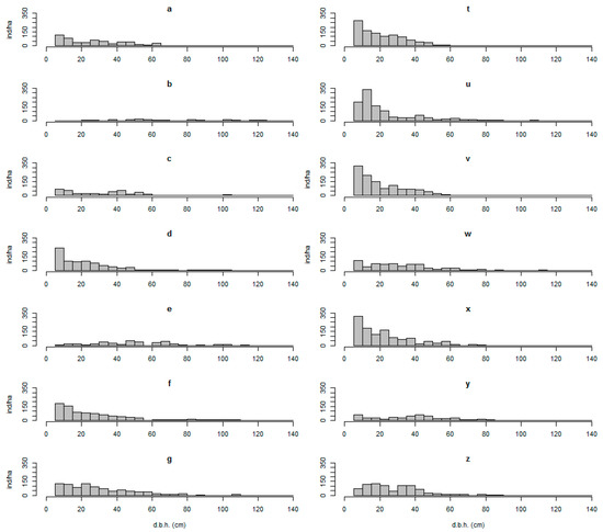
Figure 2.
Diameter distributions of the sampled plots. (a–g) Old-growth forest; (t–z) secondary forest. Letters correspond to plots, as described on Table 1.
In total, 2136 trees were measured on the ground, from which 858 trees were visualized from the UAV imagery of the canopy, with a range from 26% (Plot d) to 88% (plot b) of the measured trees (mean = 45.7%, SD = 17.3) (Figure 3). There were large differences concerning tree density and the spatial distribution of the tree diameters, which precluded the detection of certain trees (Figure 4). All in all, trees included in the UAV image mosaic represented between 70.6% (plot g) and 96% (plot b) of the total BA of the plots (mean = 80.28%, SD = 7.7); on highly diverse plots and secondary forests, the ratios were lower, ranging from 18.2% (plot v) to 88.9% (mean = 59.1%, SD = 23.5). Concerning tree species richness, when there were fewer than five tree species, all of them were represented in the UAV processed data.
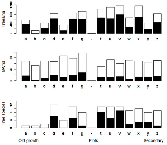
Figure 3.
Plot level variables detected using an unmanned aerial vehicle (UAV). The complete bars represent the ground data measurements of the plots. The light color represents the portion of the canopy effectively detected and the black represents the portion not visualized by the UAV imagery.
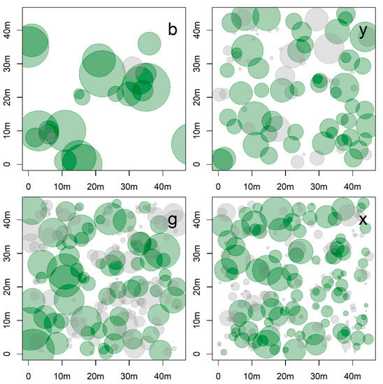
Figure 4.
Spatial distribution of the tree diameters (DBH, ground data) in four of the studied plots, representing old-growth (corresponding to plots b and g) and secondary forests (plots y and x). The plots selected denote the highest and lowest tree density in each category. The size of the circle represents tree diameters and green circles represent trees effectively detected using unmanned aerial vehicle.
3.2. Diameter Classes Represented in the Remote Sensing Data
Some plots with A. araucana were nearly monospecific (90% of BA) and were excluded from the calculations concerning the analysis of forest variables by diameter class. For the rest, the diameter classes were defined every 10 cm. The BA effectively retrieved from the UAV data was 83.6% and 83.3% on old-growth and young forests, respectively, in particular, it exceeded 70% on diameter classes over 35 and 25 cm, respectively. About 37.9% and 48.5% of individual trees were detected on old-growth and young forests, respectively, rising to over 50% for diameters over 35 and 25 cm, respectively (Figure 5).
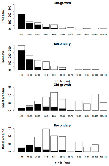
Figure 5.
Basal area (BA, m2) and density (trees ha−1) effectively detected from unmanned aerial vehicle (UAV) imagery for each diameter class (DBH, cm). Ground-based values represented by Table 3.
3.3. Stand Structure Variables
Considering the individual-tree crown data, there was a relationship between the measured QMD and the UAV-retrieved BA and density. On the one hand, for QMD, it was a positive correlation; therefore, for a higher QMD there were more trees detected (R2 = 0.71) and retrieved BA (R2 = 0.47). Density, on the other hand, presented a negative correlation; therefore, the sparser the forest, the higher the proportion of trees (R2 = 0.57) and BA (R2 = 0.37) detected by the UAV images (Figure 6).
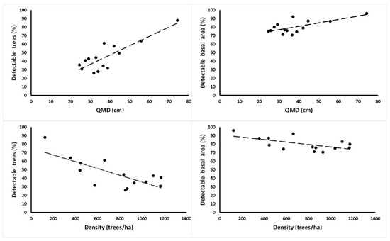
Figure 6.
Relationships between quadratic mean diameter (QMD, cm) and density (trees ha−1) versus percentage of detected trees and unmanned aerial vehicle imagery estimated basal area (BA, m2). N = 14 plots.
Significant relationships among the stand variables and the canopy structure estimates from the UAV imagery were also found. The relative forest density was related to the total canopy surface and inversely related to the standard deviation of the tree crown’s surface (R2 = 0.73, p-value < 0.05). A similar pattern was observed regarding the QMD (R2 = 0.73, p-value < 0.001). There were no observed linear relationships between the BA and the canopy structures retrieved (Table 2).
Table 2.
Linear model of (a) tree density, (b) quadratic mean diameter, and (c) basal area, related with forest canopy area and standard deviation (SD) of trees’ crown area.
3.4. Individual-Tree DBH
For the individual-tree DBH, the BRT approach estimated the between-species variability to be ca. 17% of the total, and the main variable explaining tree diameter was the tree crown area, accounting for 68.9%. Other variables tested were below 5% and were not considered at this stage. The BRT model had a high predictive power (R2 = 0.78, based on CV, R2 = 0.69). These results were further studied on a mixed model, using the tree crown area as a predictor in the fixed part of the model, and the species as the random factor (Figure 7). The predictive power of the model was R2 = 0.55 for the fixed part of the model and R2 = 0.66 for the whole model, including between-species variability (Table 3). The between-species variability was expressed in the intercept using a random parameter (Table 4); these values were related to their corresponding marginal effects on the BRT’s estimates.
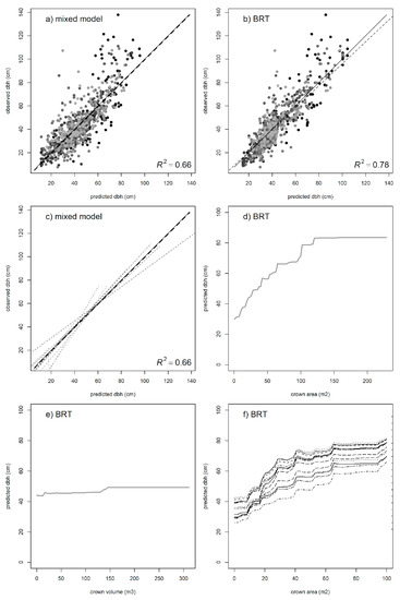
Figure 7.
Predicted DBH values for the (a) mixed model and (b) boosted regression trees (BRT). (c) Using crown area as the main variable (main effect in bold line) and incorporating between-species predictions (N = 12, discontinuous lines) as a random factor as compared with BRT marginal effects for (d) crown area, (e) crown volume, and (f) each individual species. In the mixed model, the between-species standard deviation was 6.81 for an estimated residual deviation of 12.06. The main contributions for the BRT model were crown area (68.9%), species (16.9%), and crown volume (6.97%), the others being below 5%.
Table 3.
Parameters of the mixed model for predicting individual-tree DBH based on remote sensing metrics. The coefficient of determination was R2 = 0.55 for the fixed part of the model and R2 = 0.66 when including between-species variability (standard deviation represented by σ). The bias of the fixed part was −2.28 cm (RMSE = 13.9).
Table 4.
Marginal effects of the species on the predictions in the intercepts of the mixed model (1) and on the marginal overall effects of the boosted regression trees (2).
4. Discussion
In this study, we use a UAV-DAP approach to measure basic forest attributes in secondary and old-growth native forests, including individual-tree DBH based on these attributes. Despite the complexity of native Chilean temperate forests, the results demonstrate the potential of this approach, and confirm that the approach is feasible for retrieving reliable estimates to be used in forest assessment, management, and planning. At the same time, the study identified and addressed some important limitations. In general terms, old-growth and secondary forests differ in species composition, stand age, trees basal area, density, DBH distribution and range, presence of snags, and the heterogeneity of canopy structure [43,44]. The findings reflect that, in young dense forests, the results underestimate tree density, although they reach a reasonable accuracy concerning stand basal area. This is a direct consequence of using a UAV, which obtains better estimates of the canopy visible from above, when applied to these particular stand dynamics. With increasing QMD, the first cohorts of pioneer trees are suppressed by larger trees, concentrating on most of the BA and the canopy [43,45].
At the stand level, the results show that the total forest canopy area is related to the relative density and QMD but not to the BA (p-value < 0.001). We also found a relationship between the SD of the tree crown area and relative density (p-value < 0.05), which, in this case, could help differentiate a secondary forest from an old-growth forest. On the one hand, higher forest canopy area and less SD in tree crowns are more likely attributed to a secondary forest canopy structure due to higher competition for light in younger forests. On the other hand, old-growth or mature forests are more related to a lower canopy cover and high SD of tree crowns due to gap dynamics and uneven-aged characteristics (high variability of crown sizes) [46,47]. A positive relationship between the total forest canopy area and basal area was to be expected, although it was not significant, possibly due to a high accumulation of biomass in large trees, species-based canopy closure strategies, stand development stage, structure, composition, and environmental conditions [48]. This shows that similar forest canopy areas can result in largely different stand BAs, stressing the need to better understand alternative stand characteristics related to BA in order to develop robust models. In addition, the poor response of crown volume to diameter in the models can also be explained by the fact that this variable is notoriously difficult to establish from DAP in dense forests, as the underside of the canopy is usually not well represented in a photogrammetric point cloud (as opposed to ALS). As expected, the results suggest that the use of a UAV-DAP approach presents more limitations on forests with larger diversity of tree species and a complex structure, which are, at the same time, areas subject to special conservation objectives. Moreover, for habitat or ecosystem mapping, direct mapping of individual plants and species in diverse forests is both necessary and complex [49].
The UAV-DAP approach can provide large amounts of data concerning tree canopies, through deriving 3D photogrammetric point clouds from very high overlapping UAV images (>85% overlap); however, some information concerning tree species diversity, forest structure, and understory vegetation is not easily retrieved, particularly in dense multistory tropical forests and diverse dense old-growth forests. The results quantify to a certain extent this loss, which is larger in a forest with a greater complexity in terms of tree diversity and structure [50,51], and show that canopy-based estimates achieve an average of 45% of the trees representing over 80% of the total basal area. Furthermore, we observed high variability in the species dominating the canopy versus the total species richness, with a tendency to underestimate the species, particularly on highly diverse forests. Old-growth forests under this broad definition often have a complex structure and a heterogeneous spatial arrangement that varies depending on the forest type [52,53]. As forests become largely logged and maintained in young successional stages in many areas, there is a renewed interest in the unique structural and functional characteristics of old-growth forests because of their diminishing land cover, high relevance for the conservation of regional biodiversity, and their value for global carbon storage [54].
These unique services justify efforts for an early warning detection of forest degradation [55,56]. The results confirm that changes in canopy attributes can be easily retrieved and could be used as early warnings of forest degradation detection, as several approaches defining forest degradation are linked to the loss of the main forest attributes, i.e., composition, structure, and function [57]. Forest degradation is also associated with an impact on functional forest processes, including variables such as shoot growth in woody plants, seed availability in soil seed banks, abundance of seedlings, and the age structure of common species (as compared with that expected based on the successional state of the forest and the regeneration strategy of the various species) [58]. In this context, the use of a UAV represents an alternative for detecting forest degradation processes, especially in old-growth forests. Whereas some studies suggest that forest degradation has several dimensions that are difficult to represent in a single measure, other studies have proposed grouping indicators according to the forest attributes that have been affected by degradation [57,59]. These indicators include loss of canopy cover and reduction in structural complexity, potential gaps in some diameter classes over DBH 60 cm, and a low frequency of individuals in the intermediate diameter classes [57,59].
Finally, the combination of the modeling approaches presented offers both the advantages of machine learning in exploratory analysis, variable selection, and model structure, as well as the replicability and applicability of the more conventional regression methods [60,61]; the results of both approaches were consistent and confirm the use of a UAV as a promising alternative for inventory in native forests, providing an accurate estimation of aboveground biomass concentrated in larger trees (as those are the main economic interest and often largely determine local forest management). Despite the loss of accuracy in forests with large diversity and structure [56,62], the predictions of DBH at the tree level are enough to be the basis for quantifications of total biomass and tree fractions, which has important applications in carbon assessments and forest management.
5. Conclusions
The use of a UAV to assess and monitor forest management in Chilean temperate forests in terms of both tree species diversity and forest structure is needed at the local and regional levels to understand the impacts of interventions and to develop effective management strategies for their conservation. In this study, we analyzed the use of a UAV and field-based data methods with the potential to achieve these objectives. For most studies, the availability of resources (time, money, and manpower) is the major constraint. We suggest combining the use of both field-based and remotely sensed methods to achieve that goal as these methods can be complementary, in particular in old-growth forests. Remote-sensing data should be used to predict and map the tree species diversity and stand structure at regional scales, while field inventories provide accurate information at local scales and allow validation of remotely sensed data. In the future, fields such as forest dynamics, forest species dominance in stands, mapping, and assessing forest disturbances will grow considerably with the benefits of unmanned aircraft technology. Our results suggest that drone-derived canopy variables contributed substantially to explaining patterns of structure and biodiversity in these temperate forest plots. This study provides immediate guidance for the application of these tools in forest inventory in Chilean temperate forests and describes a methodology that can support the management of their forests according to their structure. Future studies aimed at higher accuracy estimation must advance the following three objectives: (i) better tree level segmentation, (ii) precise metric functions between crown and trunk attributes at a specific forest type level, and (iii) tree-level identification of forest species. In general, the results show that, when the focus is biomass with economic value (larger trees), accurate tree-level DBH can be obtained, especially when some level of species differentiation is applied.
Author Contributions
Conceptualization, A.M. and B.M.-Y.; data curation, A.M., G.C. and M.C.; formal analysis, A.M., B.M.-Y., G.C. and M.C.; funding acquisition, A.M., A.A. and J.G.; investigation, A.M., A.A., C.Z.-E., M.C., J.G. and B.M.-Y.; methodology, A.M., B.M.-Y. and M.C.; project administration, J.G.; visualization, A.M., B.M.-Y. and G.C.; writing—original draft, A.M., C.Z.-E. and B.M.-Y.; writing—review and editing, A.M., B.M.-Y., G.C., A.A., C.Z.-E. and J.G. All authors have read and agreed to the published version of the manuscript.
Funding
This research was funded by CORFO, grant number 13IDL2-23500.
Data Availability Statement
The data presented in this study are available on request from the corresponding authors.
Acknowledgments
A.M. and C.Z. thank ANID/FONDAP/15110009. A.M. thanks ANID Postdoctoral Fondecyt project 3210101 and Dirección de Investigación of Universidad de La Frontera. A.A. thanks FONDECYT 1211051. B.M.Y. thanks the European Union’s H2020 research and innovation programme, under the Marie Sklodowska-Curie grant agreement no. 691149 (SuFoRun). This study has been done with affiliation to the Academy of Finland Flagship Forest-Human-Machine Interplay - Building Resilience, Redefining Value Networks and Enabling Meaningful Experiences (UNITE), UEF: 337127.
Conflicts of Interest
The authors declare no conflict of interest.
References
- Song, X.-P.; Hansen, M.C.; Stehman, S.V.; Potapov, P.V.; Tyukavina, A.; Vermote, E.F.; Townshend, J.R. Global land change from 1982 to 2016. Nature 2018, 560, 639–643. [Google Scholar] [CrossRef] [PubMed]
- Potapov, P.; Hansen, M.C.; Laestadius, L.; Turubanova, S.; Yaroshenko, A.; Thies, C.; Smith, W.; Zhuravleva, I.; Komarova, A.; Minnemeyer, S.; et al. The last frontiers of wilderness: Tracking loss of intact forest landscapes from 2000 to 2013. Sci. Adv. 2017, 3, e1600821. [Google Scholar] [CrossRef] [PubMed]
- Köhl, M.; Lasco, R.; Cifuentes, M.; Jonsson, Ö.; Korhonen, K.T.; Mundhenk, P.; de Jesus Navar, J.; Stinson, G. Changes in forest production, biomass and carbon: Results from the 2015 UN FAO Global Forest Resource Assessment. For. Ecol. Manag. 2015, 352, 21–34. [Google Scholar] [CrossRef]
- Whiteman, A.; Wickramasinghe, A.; Piña, L. Global trends in forest ownership, public income and expenditure on forestry and forestry employment. For. Ecol. Manag. 2015, 352, 99–108. [Google Scholar] [CrossRef]
- Iglhaut, J.; Cabo, C.; Puliti, S.; Piermattei, L.; O’Connor, J.; Rosette, J. Structure from Motion Photogrammetry in Forestry: A Review. Curr. For. Rep. 2019, 5, 155–168. [Google Scholar] [CrossRef]
- Anderson-Teixeira, K.J.; Davies, S.J.; Bennett, A.C.; Gonzalez-Akre, E.B.; Muller-Landau, H.C.; Joseph Wright, S.; Abu Salim, K.; Almeyda Zambrano, A.M.; Alonso, A.; Baltzer, J.L.; et al. CTFS-ForestGEO: A worldwide network monitoring forests in an era of global change. Glob. Chang. Biol. 2015, 21, 528–549. [Google Scholar] [CrossRef]
- Liang, J.; Crowther, T.W.; Picard, N.; Wiser, S.; Zhou, M.; Alberti, G.; Schulze, E.-D.; McGuire, A.D.; Bozzato, F.; Pretzsch, H.; et al. Positive biodiversity-productivity relationship predominant in global forests. Science 2016, 354, aaf8957. [Google Scholar] [CrossRef]
- Crowther, T.W.; Glick, H.B.; Covey, K.R.; Bettigole, C.; Maynard, D.S.; Thomas, S.M.; Smith, J.R.; Hintler, G.; Duguid, M.C.; Amatulli, G.; et al. Mapping tree density at a global scale. Nature 2015, 525, 201–205. [Google Scholar] [CrossRef]
- Glick, H.B.; Bettigole, C.; Maynard, D.S.; Covey, K.R.; Smith, J.R.; Crowther, T.W. Spatially-explicit models of global tree density. Sci. Data 2016, 3. [Google Scholar] [CrossRef]
- Mitchell, A.L.; Rosenqvist, A.; Mora, B. Current remote sensing approaches to monitoring forest degradation in support of countries measurement, reporting and verification (MRV) systems for REDD+. Carbon Balance Manag. 2017, 12, 1–22. [Google Scholar] [CrossRef] [PubMed]
- Morgan, J.L.; Gergel, S.E.; Coops, N.C. Aerial Photography: A Rapidly Evolving Tool for Ecological Management. BioScience 2010, 60, 47–59. [Google Scholar] [CrossRef]
- Bagaram, M.B.; Giuliarelli, D.; Chirici, G.; Giannetti, F.; Barbati, A. UAV Remote Sensing for Biodiversity Monitoring: Are Forest Canopy Gaps Good Covariates? Remote Sens. 2018, 10, 1397. [Google Scholar] [CrossRef]
- Getzin, S.; Wiegand, K.; Schöning, I. Assessing biodiversity in forests using very high-resolution images and unmanned aerial vehicles: Assessing biodiversity in forests. Methods Ecol. Evol. 2012, 3, 397–404. [Google Scholar] [CrossRef]
- Tomaštík, J.; Mokroš, M.; Surový, P.; Grznárová, A.; Merganič, J. UAV RTK/PPK Method—An Optimal Solution for Mapping Inaccessible Forested Areas? Remote Sens. 2019, 11, 721. [Google Scholar] [CrossRef]
- Brovkina, O.; Cienciala, E.; Surový, P.; Janata, P. Unmanned aerial vehicles (UAV) for assessment of qualitative classification of Norway spruce in temperate forest stands. Geo-Spat. Inf. Sci. 2018, 21, 12–20. [Google Scholar] [CrossRef]
- Romijn, E.; Lantican, C.B.; Herold, M.; Lindquist, E.; Ochieng, R.; Wijaya, A.; Murdiyarso, D.; Verchot, L. Assessing change in national forest monitoring capacities of 99 tropical countries. For. Ecol. Manag. 2015, 352, 109–123. [Google Scholar] [CrossRef]
- White, J.C.; Coops, N.C.; Wulder, M.A.; Vastaranta, M.; Hilker, T.; Tompalski, P. Remote Sensing Technologies for Enhancing Forest Inventories: A Review. Can. J. Remote Sens. 2016, 42, 619–641. [Google Scholar] [CrossRef]
- Goodbody, T.R.H.; Coops, N.C.; White, J.C. Digital Aerial Photogrammetry for Updating Area-Based Forest Inventories: A Review of Opportunities, Challenges, and Future Directions. Curr. For. Rep. 2019, 5, 55–75. [Google Scholar] [CrossRef]
- Puliti, S.; Solberg, S.; Granhus, A. Use of UAV Photogrammetric Data for Estimation of Biophysical Properties in Forest Stands Under Regeneration. Remote Sens. 2019, 11, 233. [Google Scholar] [CrossRef]
- Torresan, C.; Berton, A.; Carotenuto, F.; Di Gennaro, S.F.; Gioli, B.; Matese, A.; Miglietta, F.; Vagnoli, C.; Zaldei, A.; Wallace, L. Forestry applications of UAVs in Europe: A review. Int. J. Remote Sens. 2017, 38, 2427–2447. [Google Scholar] [CrossRef]
- Brach, M.; Chan, J.; Szymanski, P. Accuracy assessment of different photogrammetric software for processing data from low-cost UAV platforms in forest conditions. iForest Biogeosci. For. 2019, 12, 435–441. [Google Scholar] [CrossRef]
- Wallace, L.; Bellman, C.; Hally, B.; Hernandez, J.; Jones, S.; Hillman, S. Assessing the Ability of Image Based Point Clouds Captured from a UAV to Measure the Terrain in the Presence of Canopy Cover. Forests 2019, 10, 284. [Google Scholar] [CrossRef]
- Yang, Y.; Lee, X. Four-band Thermal Mosaicking: A New Method to Process Infrared Thermal Imagery of Urban Landscapes from UAV Flights. Remote Sens. 2019, 11, 1365. [Google Scholar] [CrossRef]
- Dandois, J.P.; Ellis, E.C. Remote Sensing of Vegetation Structure Using Computer Vision. Remote Sens. 2010, 2, 1157–1176. [Google Scholar] [CrossRef]
- Zhang, J.; Hu, J.; Lian, J.; Fan, Z.; Ouyang, X.; Ye, W. Seeing the forest from drones: Testing the potential of lightweight drones as a tool for long-term forest monitoring. Biol. Conserv. 2016, 198, 60–69. [Google Scholar] [CrossRef]
- Getzin, S.; Nuske, R.; Wiegand, K. Using Unmanned Aerial Vehicles (UAV) to Quantify Spatial Gap Patterns in Forests. Remote Sens. 2014, 6, 6988–7004. [Google Scholar] [CrossRef]
- Zielewska-Büttner, K.; Adler, P.; Ehmann, M.; Braunisch, V. Automated Detection of Forest Gaps in Spruce Dominated Stands Using Canopy Height Models Derived from Stereo Aerial Imagery. Remote Sens. 2016, 8, 175. [Google Scholar] [CrossRef]
- Mohan, M.; Silva, C.; Klauberg, C.; Jat, P.; Catts, G.; Cardil, A.; Hudak, A.; Dia, M. Individual Tree Detection from Unmanned Aerial Vehicle (UAV) Derived Canopy Height Model in an Open Canopy Mixed Conifer Forest. Forests 2017, 8, 340. [Google Scholar] [CrossRef]
- Reis, B.P.; Martins, S.V.; Fernandes Filho, E.I.; Sarcinelli, T.S.; Gleriani, J.M.; Marcatti, G.E.; Leite, H.G.; Halassy, M. Management Recommendation Generation for Areas Under Forest Restoration Process through Images Obtained by UAV and LiDAR. Remote Sens. 2019, 11, 1508. [Google Scholar] [CrossRef]
- Zahawi, R.A.; Dandois, J.P.; Holl, K.D.; Nadwodny, D.; Reid, J.L.; Ellis, E.C. Using lightweight unmanned aerial vehicles to monitor tropical forest recovery. Biol. Conserv. 2015, 186, 287–295. [Google Scholar] [CrossRef]
- Swinfield, T.; Lindsell, J.A.; Williams, J.V.; Harrison, R.D.; Agustiono; Habibi; Gemita, E.; Schönlieb, C.B.; Coomes, D.A. Accurate Measurement of Tropical Forest Canopy Heights and Aboveground Carbon Using Structure From Motion. Remote Sens. 2019, 11, 928. [Google Scholar] [CrossRef]
- Alonzo, M.; Andersen, H.-E.; Morton, D.; Cook, B. Quantifying Boreal Forest Structure and Composition Using UAV Structure from Motion. Forests 2018, 9, 119. [Google Scholar] [CrossRef]
- Goodbody, T.R.H.; Coops, N.C.; Marshall, P.L.; Tompalski, P.; Crawford, P. Unmanned aerial systems for precision forest inventory purposes: A review and case study. For. Chron. 2017, 93, 71–81. [Google Scholar] [CrossRef]
- Otero, V.; Van De Kerchove, R.; Satyanarayana, B.; Martínez-Espinosa, C.; Fisol, M.A.B.; Ibrahim, M.R.B.; Sulong, I.; Mohd-Lokman, H.; Lucas, R.; Dahdouh-Guebas, F. Managing mangrove forests from the sky: Forest inventory using field data and Unmanned Aerial Vehicle (UAV) imagery in the Matang Mangrove Forest Reserve, peninsular Malaysia. For. Ecol. Manag. 2018, 411, 35–45. [Google Scholar] [CrossRef]
- Puliti, S.; Ørka, H.; Gobakken, T.; Næsset, E. Inventory of Small Forest Areas Using an Unmanned Aerial System. Remote Sens. 2015, 7, 9632–9654. [Google Scholar] [CrossRef]
- Matese, A.; Toscano, P.; Di Gennaro, S.; Genesio, L.; Vaccari, F.; Primicerio, J.; Belli, C.; Zaldei, A.; Bianconi, R.; Gioli, B. Intercomparison of UAV, Aircraft and Satellite Remote Sensing Platforms for Precision Viticulture. Remote Sens. 2015, 7, 2971–2990. [Google Scholar] [CrossRef]
- Koh, L.P.; Wich, S.A. Dawn of drone ecology: Low-cost autonomous aerial vehicles for conservation. Trop. Conserv. Sci. 2012. [Google Scholar] [CrossRef]
- Friedman, J.H. Stochastic gradient boosting. Comput. Stat. Data Anal. 2002, 38, 367–378. [Google Scholar] [CrossRef]
- Elith, J.; Leathwick, J.R.; Hastie, T. A working guide to boosted regression trees. J. Anim. Ecol. 2008, 77, 802–813. [Google Scholar] [CrossRef] [PubMed]
- R Core Team. R: A Language and Environment for Statistical Computing; R Core Team: Vienna, Austria, 2013. [Google Scholar]
- Hijmans, R.J.; Phillips, S.; Leathwick, J.; Elith, J.; Hijmans, M.R.J. Package ‘dismo’. Circles 2017, 9, 1–68. [Google Scholar]
- Pinheiro, J.; Bates, D.; DebRoy, S.; Sarkar, D.; Team, R.C. Linear and nonlinear mixed effects models. R Package Version 2007, 3, 1–89. [Google Scholar]
- Gutiérrez, A.G.; Armesto, J.J.; Aravena, J.-C.; Carmona, M.; Carrasco, N.V.; Christie, D.A.; Peña, M.-P.; Pérez, C.; Huth, A. Structural and environmental characterization of old-growth temperate rainforests of northern Chiloé Island, Chile: Regional and global relevance. For. Ecol. Manag. 2009, 258, 376–388. [Google Scholar] [CrossRef]
- Ponce, D.B.; Donoso, P.J.; Salas-Eljatib, C. Índice de bosque adulto: Una herramienta para evaluar estados de desarrollo de bosques nativos de tierras bajas del centro-sur de Chile. Bosque (Valdivia) 2019, 40, 235–240. [Google Scholar] [CrossRef]
- Donoso, P.J.; Lusk, C.H. Differential effects of emergent Nothofagus dombeyi on growth and basal area of canopy species in an old-growth temperate rainforest. J. Veg. Sci. 2007, 18, 675–684. [Google Scholar] [CrossRef]
- Donoso, P.; Promis, Á.; Soto, D. Silviculture in Native Forests Experiences in Silviculture and Restoration in Chile, Argentina and Western USA; The Chile Initiative & OSU College of Forestry: Valdivia, Chile, 2019. [Google Scholar]
- Donoso, P.J. Crown Index: A canopy balance indicator to assess growth and regeneration in uneven-aged forest stands of the Coastal Range of Chile. For. Int. J. For. Res. 2005, 78, 337–351. [Google Scholar] [CrossRef]
- Pretzsch, H. Canopy space filling and tree crown morphology in mixed-species stands compared with monocultures. For. Ecol. Manag. 2014, 327, 251–264. [Google Scholar] [CrossRef]
- Lausch, A.; Bannehr, L.; Beckmann, M.; Boehm, C.; Feilhauer, H.; Hacker, J.M.; Heurich, M.; Jung, A.; Klenke, R.; Neumann, C.; et al. Linking Earth Observation and taxonomic, structural and functional biodiversity: Local to ecosystem perspectives. Ecol. Indic. 2016, 70, 317–339. [Google Scholar] [CrossRef]
- Asner, G.P.; Martin, R.E. Airborne spectranomics: Mapping canopy chemical and taxonomic diversity in tropical forests. Front. Ecol. Environ. 2009, 7, 269–276. [Google Scholar] [CrossRef]
- Ganivet, E.; Bloomberg, M. Towards rapid assessments of tree species diversity and structure in fragmented tropical forests: A review of perspectives offered by remotely-sensed and field-based data. For. Ecol. Manag. 2019, 432, 40–53. [Google Scholar] [CrossRef]
- Franklin, J.F.; Van Pelt, R. Spatial Aspects of Structural Complexity in Old-Growth Forests. J. For. 2004, 102, 22–28. [Google Scholar] [CrossRef]
- Spies, T.A. Ecological Concepts and Diversity of Old-Growth Forests. J. For. 2004, 102, 14–20. [Google Scholar] [CrossRef]
- Laurance, W.F.; Nascimento, H.E.M.; Laurance, S.G.; Andrade, A.; Ribeiro, J.E.L.S.; Giraldo, J.P.; Lovejoy, T.E.; Condit, R.; Chave, J.; Harms, K.E.; et al. Rapid decay of tree-community composition in Amazonian forest fragments. Proc. Natl. Acad. Sci. USA 2006, 103, 19010–19014. [Google Scholar] [CrossRef] [PubMed]
- Kutsch, W.L.; Wirth, C.; Kattge, J.; Nöllert, S.; Herbst, M.; Kappen, L. Ecophysiological Characteristics of Mature Trees and Stands—Consequences for Old-Growth Forest Productivity. In Old-Growth Forests; Wirth, C., Gleixner, G., Heimann, M., Eds.; Ecological Studies; Springer: Berlin/Heidelberg, Germany, 2009; Volume 207, pp. 57–79. ISBN 978-3-540-92705-1. [Google Scholar]
- Wirth, C. Old-Growth Forests: Function, Fate and Value—A Synthesis. In Old-Growth Forests; Wirth, C., Gleixner, G., Heimann, M., Eds.; Ecological Studies; Springer: Berlin/Heidelberg, Germany, 2009; Volume 207, pp. 465–491. ISBN 978-3-540-92705-1. [Google Scholar]
- Vásquez-Grandón, A.; Donoso, P.; Gerding, V. Forest Degradation: When Is a Forest Degraded? Forests 2018, 9, 726. [Google Scholar] [CrossRef]
- Ghazoul, J.; Burivalova, Z.; Garcia-Ulloa, J.; King, L.A. Conceptualizing Forest Degradation. Trends Ecol. Evol. 2015, 30, 622–632. [Google Scholar] [CrossRef]
- Stanturf, J.A.; Palik, B.J.; Dumroese, R.K. Contemporary forest restoration: A review emphasizing function. For. Ecol. Manag. 2014, 331, 292–323. [Google Scholar] [CrossRef]
- Xiang, W.; Hassegawa, M.; Franceschini, T.; Leitch, M.; Achim, A. Characterizing wood density–climate relationships along the stem in black spruce (Picea mariana (Mill.) B.S.P.) using a combination of boosted regression trees and mixed-effects models. For. Int. J. For. Res. 2019, 92, 357–374. [Google Scholar] [CrossRef]
- Cardil, A.; Mola-Yudego, B.; Blázquez-Casado, Á.; González-Olabarria, J.R. Fire and burn severity assessment: Calibration of Relative Differenced Normalized Burn Ratio (RdNBR) with field data. J. Environ. Manag. 2019, 235, 342–349. [Google Scholar] [CrossRef]
- Reder, S.; Waßermann, L.; Mund, J.-P. UAV-based Tree Height Estimation in Dense Tropical Rainforest Areas in Ecuador and Brazil. Gi_Forum 2019, 1, 47–59. [Google Scholar] [CrossRef][Green Version]


Publisher’s Note: MDPI stays neutral with regard to jurisdictional claims in published maps and institutional affiliations. |
© 2021 by the authors. Licensee MDPI, Basel, Switzerland. This article is an open access article distributed under the terms and conditions of the Creative Commons Attribution (CC BY) license (https://creativecommons.org/licenses/by/4.0/).