Abstract
In recent years, atmospheric PM2.5 pollution in China has become increasingly severe and exploring the relationships among its influencing factors is important in the prevention and control of air pollution. Although previous studies have identified complexity in variations in PM2.5 concentrations and recognized the interaction of multiple factors, little quantitative information is available on the evolution of the relationships among these factors, their spatial heterogeneity, and the multiscale interactions between them. In this study, geographical detector and multiscale geographically weighted regression models have been used to explore the multiscale interactions among natural and socioeconomic factors and PM2.5 concentration in China over the period 2000–2015. The results indicate that the relationship between natural factors and PM2.5 concentration is stronger than that for socioeconomic factors. The type of interaction between each factor is dominated by bivariate and nonlinear enhancement, exhibiting strong interactions between natural factors and anthropogenic factors. Although the effect of each factor on PM2.5 is complex, the relative influence of both human activities and social factors is shown to have gradually increased over time and population, agriculture, urbanization, and socioeconomic activities in general make important contributions to PM2.5. In addition, the scale of effects related to natural factors is smaller and more stable compared to the influence of human activities during the period 2000-2015. There are significant differences in the way natural factors and socioeconomic factors affect PM2.5, and there is strong non-stationarity of spatial relationships. Factors associated with topography, vegetation (NDVI), climate (temperature), natural sources, and agricultural activity are shown to be important determinants of PM2.5 across China and warrant significant attention in terms of managing atmospheric pollution. The study demonstrates that spatial differences in the direction, intensity, and scale of each factor should be accounted for to improve prevention and control measures and alleviate regional PM2.5 pollution.
1. Introduction
In the context of global climate change, with the rapid progress of global industrialization and urbanization, ecological and environmental issues such as air pollution and land degradation have become urgent problems for sustainable development [1,2,3]. PM2.5 air pollution, with both regional and complex characteristics, has become a significant challenge as the main component of air particulate pollutants, which can reduce atmospheric visibility [4], effect local climate change [5], interfere with traffic, and have serious economic impacts [6]. More importantly, numerous investigations have revealed that excessive concentrations of PM2.5 have been found to increase morbidity and mortality rates and are a major risk factor for global disease [7]. For example, in 2015, the number of premature deaths associated with PM2.5 in 161 cities in China was approximately 65.2 × 10⁴, accounting for approximately 6.92% of the total number of deaths in China in that year [8]. Therefore, identifying the key factors influencing PM2.5 and exploring their interactions is crucial for the prevention and control of air pollution.
Identifying the factors influencing PM2.5 has become an important research focus because it can help to inform more precise responses and preventive measures for PM2.5 pollution [9]. Atmospheric PM2.5 concentrations are affected by factors associated with the sources of particulate matter, transmission and diffusion [10,11,12,13]. Both direct factors, such as natural and artificial sources, and indirect factors, such as diffusion and settlement conditions and human activity intensity, have been widely studied [14,15,16]. At the regional scale, factors affecting the speed and direction of atmospheric diffusion (topography, temperature, pressure, wind speed and direction) [17,18,19] and factors related to the deposition of fine particles (humidity and precipitation) [4,13,18,20] play an important role in the transmission and diffusion of PM2.5. In addition, urban morphology [21], urbanization [22], land use [23], and other factors associated with human activities are known to strongly impact PM2.5 particle source, diffusion and depositional processes by altering local hydrothermal conditions [24] or the dynamics of source-sink landscapes [25]. The impacts of geospatial attributes and the regional economy on PM2.5 pollution have been demonstrated to have clear spatial aggregation and diffusion effects [26]. For instance, there is a strong correlation between the spatial configuration of the urban landscape and PM2.5 pollution in China, illustrating the effects of marked spatial differences in national, regional and urban agglomeration [27]. Therefore, spatial heterogeneity of PM2.5 concentrations and the processes influencing regional spatial variations must be taken into consideration when studying the mechanisms influencing PM2.5.
In recent years, researchers have quantified the relationship between various natural and socioeconomic factors and PM2.5 concentrations using ordinary least squares (OLS), spatial econometric models based on spatial autocorrelation, and nonlinear response models such as generalized additive models and random forest models [28,29,30]. However, these simulations are still in essence based on global regression models [27,31], without considering the spatial non-stationarity caused by interactions among the measured variables [32]. To this end, Wang et al. [31] applied a geographical weighted regression (GWR) model to assess regional differences in influencing factors through measuring spatial variation in the parameters. However, the relationship between the influencing factors and PM2.5 concentration varies according to spatial scale [33] which must be accounted for in analyzing the factors influencing PM2.5. Fotheringham et al. [34] emphasized the concept of multiscale geographic processes and proposed a multiscale geographically weighted regression model (MGWR) mode, based on a GWR model, which allows relationships between different variables to operate at different spatial scales by searching for different bandwidths to capture the effect of spatial scale on the different factors. We have therefore applied the MGWR model here to explore the interactions among atmospheric PM2.5 influencing factors in China.
Despite the shift from considering only a single spatiotemporal scale towards a comparative study of different spatiotemporal scales, spatiotemporal heterogeneity in the processes influencing PM2.5 remains unclear [9,30,31,33]. At larger spatial scales, few studies have managed to overcome the restrictions imposed by administrative boundaries, which makes it difficult to understand the potential correlation mechanisms underlying the pattern of PM2.5 pollution and effectively control the transfer of pollutants. Additionally, although PM2.5 has been recognized as influenced by the interaction between multiple factors, these interactions have not been quantified, and their evolution has not been studied, while the response process of PM2.5 to each factor has not been spatially resolved. The major aim of this study, therefore, is to describe and explain the multiscale interactions between natural, socioeconomic factors, and PM2.5 pollution in China. Firstly, spatial visualization of PM2.5 raster data are used to identify the spatial and temporal evolution of atmospheric PM2.5 concentrations during the period of 2000–2015. Secondly, correlation analysis and geographical detector models are used to quantify the global one-way and interactive relationship between natural, socioeconomic factors on PM2.5 concentration. Finally, the MGWR model is applied to quantify the multiscale effects of natural, socioeconomic, and land use factors on PM2.5. This study applies a novel method that is capable of accounting for the spatially explicit responses of natural and socioeconomic factors on PM2.5 concentrations that can provide accurate theoretical support for the control of PM2.5 pollution in China.
2. Materials and Methods
2.1. Data Sources and Processing
2.1.1. Annual Mean PM2.5 Concentrations
The data on PM2.5 used in this study were selected from the PM2.5 grid estimation dataset of China (V4.CH.02) simulated by the Atmospheric Composition Analysis Group with a spatial resolution of 0.01° × 0.01° (URL: http://fizz.phys.dal.ca/~atmos/martin/?page_id=140#V4.CH.02 accessed 22 September 2020). Considering that the response of PM2.5 concentrations to natural and socioeconomic factors requires a certain amount of time to develop spatial pattern changes on a large spatial scale, the data period 2000–2015 was chosen to start the study by operating in a 5-year time step (2000, 2005, 2010, 2015). This dataset uses the geophysical relationship between aerosol optical depth (AOD) and PM2.5 from NASA MODIS, MISR, SeaWIFS and other satellite instruments to estimate the concentration of PM2.5 through a chemical transport model (GEOS-Chem), and uses a GWR for calibration, with an accuracy of up to 81% [35]. Detailed information on the dataset is given in van Donkelaar et al. [35,36]. These data have been widely used in PM2.5 research [37,38].
To verify the reliability of this dataset in across China, this study uses PM2.5 concentration data monitored by 1497 ground-based monitoring stations in 2015 released by the Chinese Ministry of Ecology and Environment to compare and validate the PM2.5 raster dataset. The monitored annual average PM2.5 concentrations at the stations were spatially matched with the estimated PM2.5 concentration values through the “extract by points” tool in ArcGIS 10.2, and the correlation coefficient and root mean square error (RMSE) were calculated as 0.852 and 10.57, respectively. Han et al. [37] used this dataset to assess the accuracy of remotely sensed annual mean PM2.5 concentrations at the provincial spatial scale and, in validating the results, showed that the maximum relative error was 4.9% in 2015. Therefore, minimal information is lost in using the modelled dataset compared with the actual values of regional PM2.5 concentrations in China, and it can therefore be reliably used in the spatial analysis of regional PM2.5 concentrations in China. Regional PM2.5 pollution in China is classified by categorizing PM2.5 concentrations into five levels that relate to the annual limit of PM2.5 concentration in China’s Ambient Air Quality Standard [39] and the air quality guideline (AQG) by the World Health Organization [40]; specific classification information is shown in Figure 1.
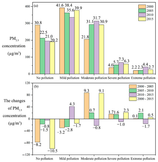
Figure 1.
The areas (a) and the changes in the areas (b) with PM2.5 concentration levels in China from 2000 to 2015. No pollution, PM2.5 concentration < 10; Mild pollution, PM2.5 concentration [10,35); Moderate pollution, PM2.5 concentration [35,70); Severe pollution, PM2.5 concentration [70,100); Extreme pollution, PM2.5 concentration ≥ 100. The numbers above each column indicate the percentage of areas with per PM2.5 concentration level relative to the total area of the entire country. The values on the graph are approximate due to rounding.
2.1.2. Influencing Factors
This study focuses on the spatial heterogeneity in response to natural and anthropogenic factors of PM2.5 concentration; therefore, based on the principle of spatial raster data accessibility, factors are selected in terms of natural factors and socioeconomic factors. Different factors are quantified using different datasets. Table 1 presents the factor categories established in this research and their corresponding application datasets. Through statistical analysis of the direction and intensity of the relationship between various factors and PM2.5 concentration, the difference in the effects of natural conditions and human activities on PM2.5 can be identified [29,30,31].

Table 1.
Description of data categories and sources.
Topographic, meteorological, vegetation, and natural source factors were selected to express the influence of natural conditions. Elevation (ELE, acquired by digital elevation model) was chosen to quantify the topographic factor, which often acts as an important spatial constraint on the transfer of airborne particulate pollution. The effects of complex topographic units such as plateaus, basins, and valleys in the Chinese region are known to be more important than that of Europe and the United States in that pollutants are less likely to be dissipated in such situations [13]. Meteorological factors are quantified using mean annual precipitation (PRE), mean annual temperature (TEM), and wind speed (WIND). Precipitation is known to affect PM2.5 in the form of a flushing effect and removing atmospheric pollutants [18]; temperature affects atmospheric convection and influences evaporative losses with a resultant influence on PM2.5 [20]; high wind speeds have the ability to both erode and disperse particles and favor PM2.5 dispersion process [4]. Vegetation cover index (NDVI), proportion of forested land (PFOL), and proportion of grassland (PGRL) were selected to quantify vegetation factors. Generally, relying on the adsorption and dust reduction effect of vegetation [41,42], there is a negative correlation between vegetation and PM2.5 concentration, while there will be some variability in effects of vegetation in general and vegetation type on PM2.5 [25]. In addition, unused or bare land and sandy land are susceptible to wind erosion and generate surface dust, making unused land an important input to PM2.5 [11]. Therefore, the proportion of unused land (PUNL) is used as a quantitative expression of natural source factors.
Three factors that directly represent the intensity of human activities (gross domestic product (GDP), population density (POP), and nighttime light intensity (NLI)) and two land use factors that indirectly reflect the intensity of human activities in rural versus urban areas (proportion of agricultural land (PFAL) and proportion of built-up land (PCOL)) are used here to represent the influence of socioeconomic activities. Population density indicates the number of people in a spatial unit, and several existing studies point to the significant contribution of population density to PM2.5 concentrations [43]. Gross domestic product (GDP) describes the economic development within a spatial unit, and in general the energy consumption and particulate emissions from regions with high population density and rapid economic development become important anthropogenic sources of PM2.5 concentrations [33,43]. NLI is widely used in the spatial quantification of urban characteristics, representing integrated urban characteristics such as population, economic dynamics, traffic levels, and city-size distribution [44,45]. Improvements in the level of urban development (demographics, economic structure, transportation layout, etc.) can alleviate the degree of PM2.5 pollution, and the Environment Kuznets Curve (EKC) in China’s cities can provide a relevant measure of this [46]. While the proportion of cultivated land can be used directly to assess agricultural activities, the crop cover of cultivated land and agricultural activities such as fertilization soil plowing and biomass burning make cultivated land a dynamic source landscape for aerosols [47,48,49]. The proportion of construction land is directly related to urbanization. Construction and industrial activities resulting from the expansion of urban construction land have become major sources of PM2.5 [50], while the rapid expansion of urban areas has amplified the intensity of the heat-island effect, thereby affecting the transmission and diffusion of PM2.5 [51].
In considering all of the variables used in this study, spatial resolution was standardized to 1 km × 1 km so that the data on various influencing factors match well with the PM2.5 data, and spatial sampling errors are minimized. The spatial location of all datasets was mediated by grid cells. Specifically, we established 23,614 grids of 20 km × 20 km size at the regional scale across China and PM2.5 data, DEM data, NDVI, meteorological data, GDP, POP, and NLI data were resampled to the spatial resolution of the grid cells to extract the corresponding resampled values of the grid cells and to calculate the proportional areas of arable land, forest land, grassland, construction land, and unused land within each grid cell. Pearson correlation coefficients between PM2.5 and influencing factors were calculated using all data attributes for each of the 23,614 grid squares as the sample set, with PM2.5 concentration values set as the dependent variable. The independent variables were input into the geographic detector and multiscale geographically weighted regression model to evaluate the spatial heterogeneity of natural and socioeconomic factors and PM2.5 concentrations.
2.2. Methods
2.2.1. Geographical Detector Model
Geographical detector modelling, an important statistical method in spatial differentiation research, is a statistical method used to describe heterogeneity in spatial stratification and reveal its internal driving factors through a nonlinear hypothesis. The model assumes that if an independent variable has a strong causal relationship with a dependent variable, then the independent variable and the dependent variable will exhibit a high degree of consistency in their spatial attributes [59]. Geographical detector models have been widely used in studies of land use, regional economies, ecology, and environmental science among others (see Wang et al. [60]). In this study, factor detectors and interaction detectors are used to address two issues, viz., which variables have a significant impact on PM2.5 concentration and how do these variables interact with each other.
In regard to the factor detector, q statistics are first used to quantify the degree of influence of a single factor and the interaction between two factors. Values of q are calculated using the following formula:
where h (1, …, L) represents the sub-region of independent variable X, represents the number of samples in the subregion of h, N represents the number of spatial units in the whole region, represents the variance of the subregion, and represents the total variance of the whole region. In this study, the sub-region represents grid cells with a spatial scale of 20 km × 20 km.
An interaction detector is used to detect the interaction between two factors. The q value is used to assess the nature of interaction between the two factors, such as whether the interaction between two factors enhances or weakens the explanatory power of the single factor on the dependent variable Y or is consistent with the effect of the two factors acting independently on Y. The interaction detector is based on the factor detector result, and is calculated as follows:
- q values of X1 and X2 obtained from equation 1 are expressed as q(X1) and q (X2);
- The two factor layers X1 and X2 are used for superposition. The new superposition factor layer after the superposition is X1∩X2, and the Equation (1) is used again to calculate the q value of X1∩X2 at the superposition factor layer, which is expressed as q(X1∩X2);
- According to the magnitude of q (X1), q (X2) and q (X1∩X2), it can be divided into five types of interaction; the specific comparison and corresponding interaction relationships are shown in Table A1.
The geographical detector R package was used in this study to calculate the factor detector and interaction detector [61].
2.2.2. Multiscale Geographically Weighted Regression Model
Classical GWR sets up a consistent bandwidth for all factors such that all the relationships operate at the same spatial scale. However, the spatial relationships between each factor and dependent variable play different roles at different scales [33], and the relationship between the factor and dependent variable is also scale dependent [62]. Therefore, Fotheringham et al. [34] developed the MGWR model based on a GWR by relaxing the hypothesis that all spatial change processes in the model operate at the same spatial scale and assigning a dedicated bandwidth for each variable to adapt the model to account for its multiscale effects. The MGWR can eliminate the limitation that all relationships must vary at the same spatial scale, minimize overfitting, and improve the accuracy and superiority of the model [63]. The MGWR is expressed as
where represents the coordinates of sample point i; and represent the dependent variable and the kth explanatory variable, respectively; represents the local parameter estimation of the kth explanatory variable of sample point i in optimal bandwidth; represents the intercept in optimal bandwidth; and represents the error term; bwk is the specific optimal bandwidth used in the calibration of the conditional relationship between the explanatory variable k and the independent variable, which means that the relationship between explanatory variables and dependent variables allows changes in space in the model and provides bandwidth parameters of optimal geographical range, thus allowing different processes to run at different spatial scales.
MGWR is essentially a multiple linear regression, and the multivariate complexity and correlation of PM2.5 concentration influencing factors, so the multiple covariance problem needs to be solved before running MGWR; the test of variance inflation factor (VIF) is the most concise variable screening method [64]. This study solves the multiple covariance problem by screening out the variables with VIF > 10. The original data were also normalized in order to make the coefficients of the modeling results statistically comparable at different locations and for different variables.
During the establishment of the MGWR model, the bandwidth was calibrated using a back-fitting algorithm [34]. In this paper, all calibration of the model was carried out using MGWR 2.2 software [63,65], which is suitable for modeling large datasets. The software is available at https://sgsup.asu.edu/sparc/multiscale-gwr accessed 22 September 2020. In order to verify the practical validity of the MGWR model, a total of 658 matched samples were obtained using the spatial connection between ground-based monitoring stations and the 20 km × 20 km grids. The results of the linear fit between the predicted values of the MGWR model and the monitored PM2.5 concentration values at the stations showed that the regression coefficient R2 of the fit reached 0.715, which means that the MGWR model implemented in this study has a reliable practical value.
3. Results
3.1. Spatio-Temporal Patterns in PM2.5 Concentration
Figure 1 shows changes in the percentage areas of each category of mean annual PM2.5 nationwide, considerably more than half of China experienced PM2.5 pollution during 2000 to 2015. Non-polluted areas exhibited a continuous decrease, while the correspondingly polluted area gradually expanded over time. Notably, areas with moderate pollution and severe pollution increased by 1.42 times and 1.57 times, respectively, during 2000–2015. The overall pattern of change in the pollution situation over the period is suggestive of three temporal phases as follows: rapid deterioration (2000–2005)/deterioration mitigation (2005–2010)/marginal improvement (2010–2015).
From 2000 to 2015, the PM2.5 concentrations exhibit substantial spatial variations; there is a clear spatial division in PM2.5 distribution across the so-called Hu Huanyong line [66] from the southeast inland to the northwest (Figure 2a–d) revealing clear spatial agglomeration. The spatial variation in moderate and severe pollution areas changed significantly during the period of 2000–2015. Severely polluted areas, centered on the arid region of northwest China, spread in a southeasterly direction over time. In addition, severe pollution areas in the industrialized provinces of the middle east (including Henan and Hebei) expanded to the southwest. Areas of moderate pollution also spread in a southwesterly direction from the areas of urban agglomerations. A clear overall pattern is apparent: the highly polluted areas of northwest China are associated with the arid dust source areas, while pollution in the central and eastern regions of China are associated with centers of urbanization and industrialization.
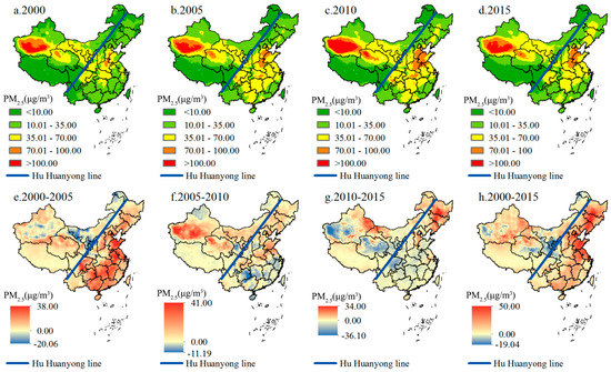
Figure 2.
Spatial pattern (a–d) and temporal trend (e–h) of PM2.5 in China from 2000–2015.
During the period of 2000–2005 (Figure 2e), the PM2.5 concentration increased across 75.1% of China, especially to the east of the Hu Huanyong Line, due to rapid urbanization. In 2005–2010 (Figure 2f), the variation in PM2.5 concentration exhibited a north-south differentiation, and the areas where the pollution situation deteriorated were mainly distributed in northern China. Between 2010 and 2015, PM2.5 concentrations increased only in some of the northern provinces, such as the eastern parts of Xinjiang, Gansu, Inner Mongolia, and Heilongjiang (Figure 2g), whereas the rest of the country (almost 50%) China showed a decreasing trend of PM2.5 concentrations, especially in western Xinjiang where significant pollution-control results have been achieved. Nevertheless, although nearly half of the country exhibited improved PM2.5 concentrations in 2015 compared to 2010, atmospheric pollution conditions were still worse than in 2000 across more than 80% of China (Figure 2h).
3.2. Correlation Analysis
Determination of Pearson’s correlation coefficient values indicate that the PM2.5 concentration is significantly correlated with the influencing factors (Table A2). For natural factors, there is a significant positive correlation between TEM, PUNL, and PM2.5 concentration, whereas the remaining factors showed a significant negative correlation. Moreover, the factor with the greatest influence on PM2.5 concentration shifted from the natural source factor PUNL to the meteorological factor WIND over the period 2000–2015; the intensity of vegetation factors and meteorological factors in terms of transport dispersion is stronger than that of natural sources in the middle and late stages. For socioeconomic factors, all factors have a very significant positive correlation with PM2.5, and the correlation has strengthened over time; the impact of human agricultural and urban activities on PM2.5 concentration is stronger than the overall socioeconomic activities, and its intensity approaches the intensity of some natural factors, indicating that human activities and urban development have an increasingly prominent influence on PM2.5 concentration. Overall, the relationships between PM2.5 concentration and natural factors are stronger than those relating to socioeconomic factors. However, over time, the influence of human activities on the PM2.5 concentration has gradually increased.
3.3. Geographical Detector Model Analysis
3.3.1. Factor Detector Analysis
The degree of influence (q value) of the spatial distribution of each influencing factor derived from the factor detector for the spatial differentiation of PM2.5 concentration indicates that all of the influencing factors have a significant impact on PM2.5 concentration (p < 0.01) and follow the sequence: natural factors > socioeconomic factors (Table 2). Among the 13 selected factors, TEM has the highest degree of influence in 2000, 2005, and 2010, with q values of 0.39, 0.35, and 0.35, respectively. The degree of influence of WIND increased sharply in 2015, with the q value reaching 0.37. It is also worth noting that the intensity of the influence of POP on PM2.5 is stronger than that of human regional activities, and the degree of influence of agricultural activities is stronger than that of urban activities, and this evidence is different from what is displayed by the correlation coefficients. In addition, the absolute value of the correlation coefficients is generally larger than the q value, and the difference between the q value of each influencing factor is larger than that of the correlation coefficients, which indicates that the effect of each influencing factor on PM2.5 is dominated by the linear effect and that the nonlinear effect of natural factors is stronger than the socioeconomic factors.
Table 2.
The q value of each influencing factor derived from the factor detector.
3.3.2. Interaction Detector Analysis
Interaction detectors are applied to identify the interaction between two influencing factors on the PM2.5 concentration among the 13 selected influencing factors (Table A3). The results show that there are two types of interactions between each pair of influencing factors during the period 2000–2015, viz., bivariate enhancement and nonlinear enhancement. As shown in Table A3, it is clear that the explanatory ability of the interaction between most factors on the spatial distribution of the PM2.5 concentration is enhanced nonlinearly. Over time, the number of dual-factor enhanced factor pairs gradually increased from 30 pairs in 2000 to 40 pairs in 2015, and the increasing factor pairs are mainly those between WIND and other factors, PGRL and socioeconomic factors. This indicates that the interaction between WIND, PGRL, and other factors has weakened, while the individual influence of each factor has been enhanced.
Factor pairs with interactive q statistic values greater than 0.5 occur between natural factors, as well as between socioeconomic factors and temperature and precipitation. Temperature and precipitation have the greatest number of high interaction factor pairs, and the interaction with temperature is the most frequent in terms of the number of occurrences. Among the socioeconomic factors, POP, GDP, and PFAL all exhibit strong interactions with precipitation. Among all factors, natural factors are still the dominant force driving the variation in PM2.5 concentration. However, the factor pairs with interaction q statistic values greater than 0.5 among the influencing factors were significantly reduced, and the difference between q values gradually decreased in 2015. The weakening of the interaction between natural factors and the strengthening of the interaction between human activities and social factors represent a change in the dominant force of natural factors and the synergistic force of socioeconomic factors (i.e., the weakening of the dominant force of nature and the strengthening of the force of human activities and social factors), and the gradual decrease in the difference in the forces of interaction reflects the gradual balance in the interaction between the factors influencing PM2.5 concentrations.
3.4. Multiscale Geographically Weighted Regression Model Analysis
The spatial bandwidth derived from the MGWR model represents the change in the spatial scale of the relationship between each influencing factor and PM2.5 concentration, and the bandwidth can be considered as the number of samples included in the local calculation. The bandwidth size determines whether the relationship between each factor and the dependent variable is local, regional, or global, on the one hand, and expresses the degree of spatial stationarity and spatial heterogeneity of each relationship, on the other hand. To classify the spatial scales of bandwidth, the number of spatial units is obtained by calculating the ratio of the total number of samples to the number of samples in the local calculation and rounding it. Comparing the number of spatial units with the number of administrative divisions at all levels in China divides that the larger regional scale > provincial division, provincial division > smaller regional scale > municipal scale, and local scale < municipal scale.
The bandwidth derived from the MGWR for 2000–2015 shows that the spatial scale at which each influencing factor operates varies (Table 3). During the period 2000–2015, only WIND, GDP, and NLI showed a shift in spatial scale range, showing the instability of spatial heterogeneity, and the fluctuation of spatial scale range only appeared at the smaller regional scale with the smaller regional scale; then, perhaps the provincial level is the key control range for WIND, GDP, and NLI factor. All other factors fluctuate and change within the same spatial scale, and the spatial heterogeneity is more stable, while the ELE has the least variation in the range of influence, indicating that the spatial heterogeneity is both stable and high and is strongest in spatial non-stationarity. The spatial influence range of vegetation factor, meteorological factor, and natural source factor is the smaller regional scale, but PUNL fluctuates more strongly in the smaller regional scale and is close to the provincial scale. Among the socioeconomic factors, the spatial influence range of POP and PCOL is the larger regional scale, and the influence range of POP is larger under the influence of population migration, while the larger regional spatial influence range of urban activities (PCOL) indicates that construction land plays an important role in the cross-regional transmission of PM2.5. It is noteworthy that agricultural activities represented by cropland have a pattern similar to the variation in NDVI, suggesting that crops and vegetation have similar effects. In general, the influence range of natural factors tends to be closer to the provincial scale at the smaller regional scale, while the influence range related to human activities is dominated by a large regional scale and forms a range fluctuation.
Table 3.
Spatial bandwidth of each variable derived from the MGWR model.
In assessing the statistical significance of the regression coefficients, at least 66.47% of the regression coefficients passed the significance test (p < 0.05) from 2000 to 2015, indicating that the regression coefficients in general are credible. Regression coefficients for each influencing factor derived from the MGWR model are shown in Table 4. In terms of the coefficient maximum ratio in all of the data, in which PCOL has a single positive effect on PM2.5 nationwide, WIND has a single negative effect on PM2.5 except in 2015, while other factors act in opposing directions in different regions much of the time. The effects of each factor on the degree of spatial heterogeneity in PM2.5 vary. The range of coefficients for all stages of ELE is the largest, illustrating the strongest degree of spatial heterogeneity. In contrast, NLI in 2000–2010 and PCOL in 2015 exhibit a low range of coefficient values, thereby suggesting minimal spatial heterogeneity degree, which is consistent with the bandwidth results. In terms of the average value of various indicators, the factor that has the greatest impact on PM2.5 changes from PRE (2000) to WIND (2005 and 2010) to PFAL (2015). Considering the regression coefficients for socioeconomic factors, the effect of human activity at the regional scale, represented by cultivated land and construction land, is much stronger than for all the regional socioeconomic indicators; the sequence of the intensity of effect is PFAL > PCOL.
Table 4.
Coefficients of independent variables derived from the MGWR model.
4. Discussion
4.1. The Advantages of the MGWR Model in Quantifying the Relationship between Factors and PM2.5 Concentration
Referring to Tu et al. [27], the coefficient of determination (R2), adjusted R2, Akaike information criterion (AIC), corrected Akaike information criterion (AICc), and residual sum of squares (RSS) were selected to compare the fit of the MGWR model degree (Table 5). Through comparison, it is found that the R2 and adjusted R2 of the MGWR are much higher than the OLS model, while the AICc and RSS are much lower than the OLS model, which indicates that the MGWR model performs better in the goodness of fit for spatial elements. This has also been shown before, in the comparison of model advantages of the OLS and the MGWR in the evaluation of the impact of air pollution in China by Fotheringham et al. [67], although in this case the degree of change in the AICc and the RSS from the OLS to the MGWR model is, however, much greater than in that study. In addition, the fitting ability of the MGWR model applied in our study has emerged as superior to that of the GWR [27], PCA-GWR [64], and SEM [28] models.
Table 5.
Comparison of the parameters in the MGWR and OLS models during the period of 2000–2015.
A previous study also used the global Moran’s I to perform analysis of the residuals of models to determine consistency of the residual results against the assumptions [68] and to determine whether the model has the ability to solve the problem of spatial autocorrelation. In this study, the Moran’s I of the residuals (MIR) indicates very significant positive spatial autocorrelation in the OLS model. However, the values of the MIR in the MGWR model show a very low degree of spatial autocorrelation. This indicates that the MGWR model can solve for the spatial autocorrelation problem well in quantifying the spatial relationship between various factors and PM2.5 concentration [27,67,68]. By comparison with Tu et al. [27] the MIR of the MGWR model in this study was closer to 0 and more random, which effectively eliminates the spatial autocorrelation of each variable and indicates that the results are more reliable.
4.2. Drivers of PM2.5 Concentration in China
The MGWR model achieves the characteristic of spatial heterogeneity of the relationship between factors and PM2.5 at different spatial locations, focusing on solving the spatial non-stationarity of the relationship between factors and PM2.5, as manifested by the spatial distribution of the regression coefficients of each factor from the model output. In this part, the spatial effects of each driver of PM2.5 concentration in the Chinese region are explored by taking the MGWR model output coefficients in 2015 as an example.
There are significant differences in the way natural factors and socioeconomic factors affect PM2.5. The relationship between each factor and PM2.5 and its absolute intensity, spatial act extent scale, spatial trend of coefficients, and major influence areas can be obtained from Table 6, and spatial visualization information can be seen in Figure 3 (only for sample points in which all significance tests of the factor coefficients passed). In terms of influence range, the scope of human socioeconomic and urban activities is obviously wider than that of natural factors. In terms of the direction of influence, the socioeconomic factors act mainly in one direction, while the natural factors have positive and negative spatial non-stationarity on PM2.5 concentrations across China. In this way, the non-stationarity of the spatial relationship between PM2.5 and its influencing factors is relatively strong.
Table 6.
Comparison of spatial heterogeneity in the relationship between natural, socioeconomic factors, and PM2.5 concentration and summary of important information.
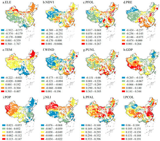
Figure 3.
The spatial distribution of regression coefficients between factors and PM2.5 concentration (samples with coefficient significance > 0.05 have been excluded). (a) The spatial distribution of regression coefficients of ELE; (b) The spatial distribution of regression coefficients of NDVI; (c) The spatial distribution of regression coefficients of PFOL; (d) The spatial distribution of regression coefficients of PRE; (e) The spatial distribution of regression coefficients of TEM; (f) The spatial distribution of regression coefficients of WIND; (g) The spatial distribution of regression coefficients of PUNL; (h) The spatial distribution of regression coefficients of GDP; (i) The spatial distribution of regression coefficients of POP; (j) The spatial distribution of regression coefficients of NLI; (k) The spatial distribution of regression coefficients of PFAL; (l) The spatial distribution of regression coefficients of PCOL. ELE, elevation; NDVI, vegetation coverage index; PFOL, proportion of forestland; PRE, precipitation; TEM, temperature; WIND, wind speed; PUNL, proportion of unused land; GDP, gross domestic product; POP, population density; NLI, night light intensity; PFAL, proportion of farmland; PCOL, proportion of construction land.
Taken at the largest spatial scale (i.e., China as a whole), the degree of influence was determined by the average of the absolute values of each factor coefficient, and the order of intensity of each factor on PM2.5 was agricultural activity factor > natural source factor > topography factor > vegetation factor > urban activity factor > meteorological factor > socioeconomic activity factor (Table 6). PUNL as a natural source factor is the most influential of the natural factors on PM2.5, which may be associated with the sand and dust activities in the large deserts in the northwest and southwest. Moreover, the overall vegetation factor (NDVI) was observed to have a stronger effect on PM2.5 than the single vegetation factor (PFOL), which may be related to the strong controlling effect of vegetation on dust activity in northwest China [69]. Another finding is that the degree of influence of arable land versus construction land is widely different but similarly stronger than meteorological factors and socioeconomic activities. Both studies at both the national and urban regional scale have indicated that farmland and construction land both play important roles in PM2.5 concentration [48,50], then different land management of urban and agricultural land may be more effective than economic management for PM2.5 management more effectively and with more accessibility than meteorological control.
The factors with the top two absolute values of the coefficients at each location were considered as the determining influencing factors at that location. The map shown in Figure 4 indicates the spatial heterogeneity of determining factors in China, and different colors represent different factors. In terms of the spatial proportions controlled by each principal factor, the topographic, vegetation (NDVI), meteorological (TEM), natural source factor, and agricultural activity factor are the factors that need obvious attention in the Chinese region. However, it should be noted that other pollutants (especially secondary-formed sulfate particulate matter) account for a considerable proportion of fine particulate matter (PM2.5), with a contribution of 36.1% from secondary sources in Beijing [70]. This study did not include secondary particulate matter in the model calculations and did not distinguish artificial sources separately. The spatial distribution of the main control factors only distinguishes the strength of the spatial relationship between different natural and socio-economic factors, and the PM2.5 concentration can identify the key factors in the variation of PM2.5 concentration from the perspective of spatial heterogeneity and cannot distinguish absolutely the spatial location of natural and anthropogenic sources.
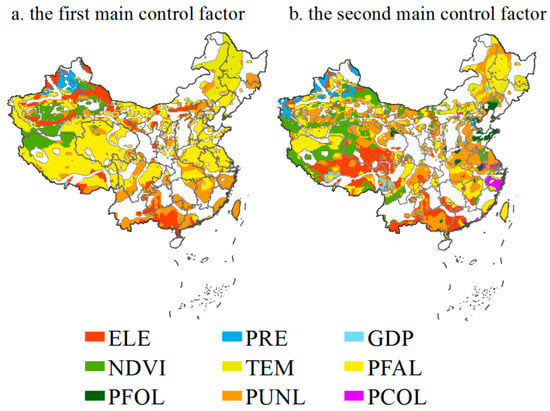
Figure 4.
The spatial distribution of main control factors in different locations in China. (a) The spatial distribution of the first main control factors; (b) The spatial distribution of the second main control factors. ELE, elevation; NDVI, vegetation coverage index; PFOL, proportion of forestland; PRE, precipitation; TEM, temperature; PUNL, proportion of unused land; GDP, gross domestic product; PFAL, proportion of farmland; PCOL, proportion of construction land.
Geomorphology is thought to influence PM2.5 accumulation and enhance pollution [17], and some studies indicate that topographic factors have the greatest effect on PM2.5 concentrations in southwest China [30], which overlaps spatially with the ELE spatial distribution results in Figure 4, but southwest China has low pollution levels except for the Sichuan basin, which is not a pollution management control area. In contrast, the pollution in Xinjiang region is serious, and the ELE on PM2.5 is clearly visible in the basin topography effect.
It is widely accepted that vegetation plays an important role in alleviating PM2.5 pollution for a range of reasons, and in this study, it can be shown that the intensity of vegetation factor in the northwest is almost twice as strong as that in the eastern and southern regions (Figure 3b). While desertification is serious in the northwest, vegetation cover is low, and dust storms are the main sources of PM2.5 concentration in the region [71]; therefore, the vegetation in the northwest exhibits a strong negative effect on dust storm activity by stabilizing the sandy surfaces [69] and increasing vegetation cover through afforestation is regularly practiced in the control of PM2.5 in northwest China [72]. Meanwhile, for PM2.5 natural sources, the proportion of natural sources (sand storms) of PM2.5 in northwestern cities increases from east to west and is less directly affected by human activities [11], and from the distribution of the main first control factor (Figure 4a) and the second control factor (Figure 4b) in the northwest, the trend of the intensity of the impact of unused land is consistent with the trend of the proportion of natural sources, but in some regions, the impact of cropland and vegetation is stronger. This may depend on the prevalence of planting vegetation to provide root anchorage and wind break to stabilize unused land surface in northwest China or through the use of straw lattice panels, which can significantly reduce PM2.5 pollution levels [69,71]. Li and Huang [48] also indicated that agricultural activities in small urban cities are more important sources of pollution compared to large cities.
The effect of PUN is shown to be the first control factor in the south, while it is the second control factor in the east (Figure 4). In the southern and eastern regions, the occurrence of even relatively small areas of unused land appears to have a strong positive effect on pollution, indicating that any increase in the area of unused land in this region may cause a substantial change in PM2.5 concentrations. It is necessary, therefore, to consider carefully the transfer of unused land to prevent deterioration in air quality. It is important to note the impact of cultivated land in the central-eastern region. The scope of the contribution of cropland to PM2.5 concentrations is limited by the space of agricultural activities and the effect of crop cover [73], and its bandwidth is shown to be narrower than that of other human activities. In addition, cultivated land is a dynamic source-sink landscape, and rapid changes in land use/cover and human activities bring about changes in temperature and humidity constraints on atmospheric dispersion in the central and eastern regions [74], reinforcing the cropland source effect.
In addition, meteorological factors tend to interact with topography [13], and the negative effect of TEM on PM2.5 is more pronounced in southwest China (Figure 3e), which may be due to atmospheric convection caused by higher temperatures here that accelerates the diffusion of particulate matter [20]. The positive high intensity of TEM makes TEM the dominant control condition in northeast China (Figure 3e and Figure 4a), according to Li et al. [75]. The Shenyang study attributed the positive TEM effect to the effect of inversion temperature on PM2.5 diffusion triggering accumulation. While PRE and WIND among meteorological factors are weak in intensity compared to other factors, the role of PRE in northwest of Xinjiang is not negligible (Figure 3d). Wang et al. [13] pointed out that strong precipitation has a significant scavenging effect by wet deposition on PM2.5 concentrations and weak precipitation and rain and fog processes may trigger air stagnation conditions. Although the annual precipitation under arid climate conditions in Northwest China is low, the intensity of precipitation is mainly high intensity and moderate intensity [76], while the intensity and frequency of precipitation show an increasing trend [77], and the important scavenging role of strong precipitation on PM2.5 in Northwest China can be speculated.
Spatial trends in GDP and NLI (Figure 3h,i) correlate with the spatial pattern of urbanization development in China. The results suggest that controlling pollution to improve atmospheric quality can be achieved in parallel with economic development, and the improvement of the integrated level of cities (population structure, economic structure, traffic layout, etc.) can mitigate the degree of PM2.5 pollution. Earlier studies applied a semiparametric spatial autoregressive model to show that the Environmental Kuznets Curve (EKC) for Chinese cities has crossed the inflection point and again suggests that higher urbanization levels can alleviate haze pollution [46]. The effect of population density on PM2.5, on the other hand, needs special treatment because the positive effect of population impact contrasts with the population density distribution [78], suggesting that a particular increase in population may trigger a greater increase in PM2.5 concentration in the more sparsely populated western areas, while the role of anthropogenic pollution sources in the east is weakened.
4.3. Interactions of PM2.5 Influencing Factors and Spatial Multiscale Relationships on PM2.5 Pollution Control in China
PM2.5 concentrations in China are affected by a combination of multiple factors, among which, on average, natural factors play a dominant role; socioeconomic factors are synergistic, however, and human activities must be taken into account. This finding concurs with other studies that have analyzed the factors influencing air quality in China [79], confirming that natural conditions act to regulate PM2.5 on a large spatial scale. However, at large scales, natural factors are not easily manipulated or managed and may not therefore be suitable targets for longer-term governance measures. In terms of socioeconomic factors in general, population tends to make a dominant contribution while, on the other hand, agricultural activities are important contributing activities to PM2.5 in China. Moreover, the interaction between socioeconomic and natural factors has been shown to play an important and significant role in the PM2.5 concentration change system [80]. It should therefore be possible to consider the identified factor pairs which exhibit strong interactions between natural factors and anthropogenic factors in managing aerosol pollution. Anthropogenic drivers are shown here to be gradually increasing in dominance over all other factors as demonstrated, for example, by the interaction detector model (Table A3), which clearly shows that the interaction between GDP, POP, PRE, and TEM can explain as much as 55.1% of PM2.5. Interactions between PFAL, TEM, and WIND can also exceed 50%, demonstrating nonlinearity of response. It is therefore suggested that the structure and spatial distribution of industry, population and distribution of farmland, for example, should be considered if the goal of regulating PM2.5 pollution is to be achieved.
This study has demonstrated that most PM2.5 influencing factors are scale dependent (Table 3) and that, as PM2.5 pollution increases, the influence of regional transmission is enhanced, while the influence of local and surrounding emission sources is reduced [10]. In addition, several econometric spatial analyses factors that influence PM2.5 in urban agglomerations and economic zones have emphasized the spatial spillover effect of PM2.5 pollution [28,29], indicating that the key to the control of PM2.5 pollution in China lies in joint governance between regions. Accordingly, the advantages of the spatial non-stationarity of the MGWR and the division of spatial act scales in this study can provide a reference for categorizing joint governance strategies level by level and provide more detailed management decisions for joint regional governance rather than a one-size-fits-all approach for all factors and all regions. For example, NDVI, PFAL, PUNL, TEM, PRE, and PCOL are selected as the key regulatory conditions of the treatment measures according to the main factor types and spatial distribution, and the strong action area of each factor is used as the center; then, the scope of treatment is determined according to its spatial bandwidth whether it is a joint treatment of cities in the province or a joint treatment of regions between provinces. Specifically, management needs to emphasize the limiting role of natural conditions and continue to promote vegetation restoration projects in the western parts of the country, while not neglecting the role of arable land contribution in small and medium-sized cities. In eastern China, the spatial layout of arable and construction land needs to be considered in relation to the distribution of industry and the source-sink system in the landscape so as to account for the interaction with natural conditions; at the same time, arable land and construction land should be managed separately and in a focused manner according to the spatial location of their intensity centers and their scale of action. In general, the study indicates that within a region, a reasonable policy should be applied to plan its control center and joint scope according to specific regional natural conditions, in the context of dominant human activities in a region such as industry, agriculture, and population etc., and to plan its important control and regulation factors by factor and sub-region to better achieve regional prevention and control of atmospheric pollution objectives.
4.4. Limitations and Future Work Directions
Without doubt, this study has some limitations. More detailed socioeconomic data including information on road traffic, industrial structure, and anthropogenic emissions are not readily available in a rasterized format and were excluded in this study. The mechanisms influencing PM2.5 impact mechanism are complex, and the selected impact factors appear to be multi-correlated. While this study uses geographic detectors to analyze the interaction among factors, how the multi-correlation between variables affects the model should be considered in the future. Multiple validation of the linear and nonlinear relationships of influencing factors on PM2.5 would be a fruitful research direction. In the future, as the understanding of the geospatial relationship between each factor and PM2.5 increases, remote sensing inversion for PM2.5 may provide corresponding information to improve the inversion model. Revealing important spatial relationships, such as vegetation factors, can be done by extracting the corresponding spectral information from satellite remote sensing in multiple directions in more detail to obtain special data products (vegetation structure, vegetation growth, crop growth) to optimize model variables.
5. Conclusions
This study was conducted to explore the interaction, spatial heterogeneity and multiscale interaction between natural and socioeconomic factors and atmospheric PM2.5 concentrations in China using geographical detector and MGWR modelling. The results indicate that the PM2.5 concentration has followed a sequence of rapid deterioration–deterioration mitigation–slight improvement during 2000 to 2015, and obvious spatial agglomeration characteristics are evident over the period. A clear spatial pattern of PM2.5 expansion across the Hu Huanyong line from the southeast coast to the northwest interior is apparent. Generally, the influence of natural factors on PM2.5 is stronger than socioeconomic factors; the effect of each influencing factor on PM2.5 is dominated by the linear effect, and the interaction type of each factor is dominated by bivariate enhancement and nonlinear enhancement, exhibiting strong interactions between natural factors and anthropogenic factors. Simultaneously, the prominent influence of natural factors is shown to weaken over time, while the effects of human activities and social factors are increasing. The contribution of socioeconomic activities in driving the system must be taken into account while agricultural activities also make important contribution to PM2.5. The analysis also demonstrates the scale dependency of many of these processes and interactions over the period 2000–2015; the influence range of natural factors tends to be closer to the provincial scale at the small regional scale, while the influence range related to human activities is dominated by a large regional scale and forms a range fluctuation. There are significant differences in the way natural factors and socioeconomic factors affect PM2.5, and the non-stationarity of spatial relationships is stronger. Topographic, vegetation (NDVI), meteorological (TEM), natural source factors, and agricultural activity factors are the factors that need significant attention in Chinese regions. In addition, the study verified that higher urbanization levels can mitigate haze pollution, while the population in western regions needs to be treated with caution, and differential land management between arable land and construction land is recommended. Management decisions for atmospheric PM2.5 concentrations should take into account both spatial heterogeneity and scale and should use reasonable policies to plan their control centers and joint scopes according to specific regional natural conditions and in combination with dominant human activities. The results here provide important information for the prevention and control of regional PM2.5 pollution in China with a categorized joint management strategy level by level.
Author Contributions
Conceptualization, X.X. and T.W.; methodology, L.Z.; resources, J.Z. and G.J.; writing—original draft, L.Z. and T.W.; supervision, M.E.M. and C.W.; project administration, X.X. and L.P.; funding acquisition, T.W. and J.Z. All authors have read and agreed to the published version of the manuscript.
Funding
This work was funded by the National Natural Science Foundation of China (41871083), Natural Science Foundation of Zhejiang Province, China (LQ21D010007, LY19D010007, LQ19D010007), and the Open Fund of Key Laboratory of Coastal Zone Exploitation and Protection, Ministry of Natural Resources (2019CZEPK09).
Institutional Review Board Statement
Not applicable.
Informed Consent Statement
Not applicable.
Data Availability Statement
No new data were created or analyzed in this study. Data sharing is not applicable to this article.
Acknowledgments
The authors would like to thank Atmospheric Composition Analysis Group [52] (http://fizz.phys.dal.ca/ accessed 22 September 2020), National Earth System Science Data Center, National Science & Technology Infrastructure of China [54] (http://www.geodata.cn/ accessed on 30 May 2021), the Resource and Environmental Science and Data Center of the Chinese Academy of Sciences [53] (http://www.resdc.cn/ accessed 22 September 2020) for providing data support. The national boundary data of China used in this study were provided by National Geomatics Center of China (http://www.ngcc.cn/ngcc accessed on 22 September 2020). The authors are grateful to the comments provided by the Editor and three anonymous reviewers, which were used to improve the quality of this work.
Conflicts of Interest
The authors declare no conflict of interest.
Appendix A
Table A1.
The category and determination of the interaction between two factors.
Table A1.
The category and determination of the interaction between two factors.
| Type of Interaction | Judging Description |
|---|---|
| Nonlinearly weakened | q(X1∩X2) < Min(q(X1), q(X2)) |
| Univariate nonlinearly weakened | Min(q(X1), q(X2)) < q(X1∩X2) < Max(q(X1), q(X2)) |
| Bivariate enhancement | q(X1∩X2) > Max(q(X1), q(X2)) |
| Independent | q(X1∩X2) = q(X1) + q(X2) |
| Nonlinearly enhanced | q(X1∩X2) > q(X1) + q(X2) |
Table A2.
Pearson correlation coefficient between PM2.5 and influencing factors.
Table A2.
Pearson correlation coefficient between PM2.5 and influencing factors.
| Factors | PM2.5 | |||||
|---|---|---|---|---|---|---|
| 2000 | 2005 | 2010 | 2015 | |||
| Natural factors | Terrain factors | ELE | −0.258 ** | −0.342 ** | −0.321 ** | −0.376 ** |
| Vegetation factors | NDVI | −0.318 ** | −0.184 ** | −0.207 ** | −0.249 ** | |
| PFOL | −0.276 ** | −0.196 ** | −0.244 ** | −0.253 ** | ||
| PGRL | −0.29 ** | −0.392 ** | −0.363 ** | −0.417 ** | ||
| Meteorological factors | PRE | −0.267 ** | −0.093 ** | −0.141 ** | −0.085 ** | |
| TEM | 0.305 ** | 0.416 ** | 0.370 ** | 0.296 ** | ||
| WIND | −0.156 ** | −0.273 ** | −0.186 ** | −0.505 ** | ||
| Natural source factor | PUNL | 0.439 ** | 0.313 ** | 0.360 ** | 0.393 ** | |
| Socioeconomic factors | Human socioeconomic activities factors | GDP | 0.054 ** | 0.186 ** | 0.155 ** | 0.103 ** |
| POP | 0.101 ** | 0.289 ** | 0.159 ** | 0.165 ** | ||
| NLI | 0.071 ** | 0.152 ** | 0.148 ** | 0.171 ** | ||
| Human regional activities factors | PFAL | 0.137 ** | 0.284 ** | 0.251 ** | 0.275 ** | |
| PCOL | 0.150 ** | 0.265 ** | 0.242 ** | 0.279 ** | ||
** significant at the 0.01 level (two-tailed).
Table A3.
The q value of each pair of interaction derived from the interaction detector.
Table A3.
The q value of each pair of interaction derived from the interaction detector.
| Factors | Year | ELE | NDVI | PFOL | PGRL | PRE | TEM | WIND | PUNL | GDP | POP | NLI | PFAL |
|---|---|---|---|---|---|---|---|---|---|---|---|---|---|
| NDVI | 2000 | 0.479 * | |||||||||||
| 2005 | 0.440 * | ||||||||||||
| 2010 | 0.427 * | ||||||||||||
| 2015 | 0.513 * | ||||||||||||
| PFOL | 2000 | 0.349 * | 0.305 # | ||||||||||
| 2005 | 0.322 * | 0.251 * | |||||||||||
| 2010 | 0.343 * | 0.253 * | |||||||||||
| 2015 | 0.40 * | 0.289 # | |||||||||||
| PGRL | 2000 | 0.266 # | 0.347 # | 0.298 * | |||||||||
| 2005 | 0.269 # | 0.348 # | 0.308 * | ||||||||||
| 2010 | 0.269 # | 0.320 # | 0.319 * | ||||||||||
| 2015 | 0.315 # | 0.404 # | 0.391 * | ||||||||||
| PRE | 2000 | 0.573 * | 0.455 # | 0.444 # | 0.478 # | ||||||||
| 2005 | 0.473 * | 0.308 # | 0.285 * | 0.369 # | |||||||||
| 2010 | 0.467 * | 0.269 # | 0.289 * | 0.356 # | |||||||||
| 2015 | 0.552 * | 0.336 # | 0.367 * | 0.435 # | |||||||||
| TEM | 2000 | 0.559 * | 0.551 # | 0.515 * | 0.398 # | 0.598 # | |||||||
| 2005 | 0.600 * | 0.503 # | 0.515 * | 0.429 # | 0.499 # | ||||||||
| 2010 | 0.586 * | 0.508 # | 0.534 * | 0.432 # | 0.540 # | ||||||||
| 2015 | 0.506 * | 0.478 * | 0.464 * | 0.393 # | 0.516 * | ||||||||
| WIND | 2000 | 0.337 * | 0.474 * | 0.351 * | 0.185 * | 0.409 * | 0.588 * | ||||||
| 2005 | 0.394 * | 0.388 * | 0.329 * | 0.280 * | 0.456 * | 0.406 # | |||||||
| 2010 | 0.372 * | 0.366 * | 0.297 * | 0.251 * | 0.479 * | 0.417 * | |||||||
| 2015 | 0.465 # | 0.484 # | 0.4687 * | 0.427 # | 0.522 # | 0.501 # | |||||||
| PUNL | 2000 | 0.420 * | 0.311 # | 0.299 # | 0.286 # | 0.452 # | 0.528 # | 0.421 * | |||||
| 2005 | 0.407 * | 0.265 # | 0.255 * | 0281 # | 0.315 # | 0.497 # | 0.360 * | ||||||
| 2010 | 0.413 * | 0.246 # | 0.263 * | 0.278 # | 0.297 # | 0.510 # | 0.368 * | ||||||
| 2015 | 0.472 * | 0.296 # | 0.296 # | 0.334 # | 0.358 # | 0.437 # | 0.477 # | ||||||
| GDP | 2000 | 0.336 * | 0.376 * | 0.161 * | 0.226 * | 0.531 * | 0.484 * | 0.222 * | 0.340 * | ||||
| 2005 | 0.3673 * | 0.403 * | 0.236 * | 0.269 # | 0.452 * | 0.474 * | 0.286 * | 0.394 * | |||||
| 2010 | 0.368 * | 0.338 * | 0.210 * | 0.253 # | 0.432 * | 0.486 * | 0.247 * | 0.368 * | |||||
| 2015 | 0.386 * | 0.424 * | 0.239 * | 0.303 # | 0.474 * | 0.448 * | 0.471 * | 0.425 * | |||||
| POP | 2000 | 0.338 * | 0.397 * | 0.195 * | 0.251 * | 0.551 * | 0.506 * | 0.272 * | 0.358 * | 0.106 * | |||
| 2005 | 0.376 * | 0.435 * | 0.282 * | 0.318 # | 0.466 * | 0.497 # | 0.340 * | 0.412 * | 0.186 # | ||||
| 2010 | 0.363 * | 0.382 * | 0.252 * | 0.286 # | 0.454 * | 0.517 * | 0.308 * | 0.390 * | 0.147 # | ||||
| 2015 | 0.396 * | 0.432 * | 0.282 * | 0.326 # | 0.503 * | 0.461 * | 0.485 # | 0.434 * | 0.173 # | ||||
| NLI | 2000 | 0.178 # | 0.264 * | 0.103 * | 0.130 # | 0.442 * | 0.344 * | 0.050 * | 0.258 * | 0.043 # | 0.081 # | ||
| 2005 | 0.189 # | 0.238 * | 0.098 * | 0.197 # | 0.301 * | 0.361 # | 0.139 * | 0.240 * | 0.120 # | 0.169 # | |||
| 2010 | 0.189 # | 0.228 * | 0.114 * | 0.179 # | 0.305 * | 0.370 # | 0.091 * | 0.251 * | 0.088 # | 0.137 # | |||
| 2015 | 0.221 # | 0.295 * | 0.143 * | 0.231 # | 0.345 * | 0.313 # | 0.401 # | 0.300 * | 0.099 # | 0.151 # | |||
| PFAL | 2000 | 0.280 * | 0.360 * | 0.129 # | 0.214 * | 0.515 * | 0.478 * | 0.183 * | 0.336 * | 0.082 # | 0.114 # | 0.055 # | |
| 2005 | 0.278 * | 0.370 * | 0.175 * | 0.240 # | 0.392 * | 0.476 * | 0.243 * | 0.356 * | 0.167 # | 0.203 # | 0.111 # | ||
| 2010 | 0.284 * | 0.338 * | 0.166 * | 0.232 # | 0.379 * | 0.490 * | 0.195 * | 0.351 * | 0.138 # | 0.174 # | 0.095 # | ||
| 2015 | 0.325 * | 0.408 * | 0.193 * | 0.284 # | 0.431 * | 0.438 * | 0.449 # | 0.402 * | 0.146 # | 0.190 # | 0.119 # | ||
| PCOL | 2000 | 0.198 # | 0.302 * | 0.115 # | 0.143 # | 0.487 * | 0.369 * | 0.079 * | 0.295 * | 0.053 # | 0.086 # | 0.034 # | 0.067 # |
| 2005 | 0.209 # | 0.308 * | 0.133 # | 0.213 # | 0.369 * | 0.388 # | 0.197 * | 0.305 * | 0.134 # | 0.177 # | 0.089 # | 0.127 # | |
| 2010 | 0.209 # | 0.285 * | 0.139 # | 0.196 # | 0.365 * | 0.363 # | 0.133 * | 0.305 * | 0.107 # | 0.142 # | 0.079 # | 0.113 # | |
| 2015 | 0.148 # | 0.367 * | 0.175 # | 0.249 # | 0.415 * | 0.366 * | 0.426 # | 0.373 * | 0.119 # | 0.167 # | 0.103 # | 0.136 # |
* The nonlinear enhancement interaction; # the Bivariate enhancement interaction.
References
- Caplin, A.; Ghandehari, M.; Lim, C.; Glimcher, P.; Thurston, G. Advancing environmental exposure assessment science to benefit society. Nat. Commun. 2019, 10, 1236. [Google Scholar] [CrossRef] [PubMed]
- Xie, X.F.; Wu, T.; Zhu, M.; Jiang, G.J.; Xu, Y.; Wang, X.H.; Pu, L.J. Comparison of random forest and multiple linear regression models for estimation of soil extracellular enzyme activities in agricultural reclaimed coastal saline land. Ecol. Indic. 2021, 120, 106925. [Google Scholar] [CrossRef]
- Xie, X.F.; Pu, L.J.; Zhu, M.; Meadows, M.; Sun, L.C.; Wu, T.; Bu, X.G.; Xu, Y. Differential effects of various reclamation treatments on soil characteristics: An experimental study of newly reclaimed tidal mudflats on the east China coast. Sci. Total Environ. 2021, 768, 144996. [Google Scholar] [CrossRef] [PubMed]
- Khanna, I.; Khare, M.; Gargava, P.; Khan, A.A. Effect of PM2.5 chemical constituents on atmospheric visibility impairment. J. Air Waste Manag. 2018, 68, 430–437. [Google Scholar] [CrossRef] [PubMed]
- Tai, A.P.K.; Mickley, L.J.; Jacob, D.J.; Leibensperger, E.M.; Zhang, L.; Fisher, J.A.; Pye, H.O.T. Meteorological modes of variability for fine particulate matter (PM2.5) air quality in the united states: Implications for PM2.5 sensitivity to climate change. Atmos. Chem. Phys. 2012, 12, 3131–3145. [Google Scholar] [CrossRef]
- Yang, S.Y.; Fang, D.L.; Chen, B. Human health impact and economic effect for PM2.5 exposure in typical cities. Appl. Energ. 2019, 249, 316–325. [Google Scholar] [CrossRef]
- Cohen, A.J.; Brauer, M.; Burnett, R.; Anderson, H.R.; Frostad, J.; Estep, K.; Balakrishnan, K.; Brunekreef, B.; Dandona, L.; Dandona, R.; et al. Estimates and 25-year trends of the global burden of disease attributable to ambient air pollution: An analysis of data from the global burden of diseases study 2015. Lancet 2017, 389, 1907–1918. [Google Scholar] [CrossRef]
- Maji, K.J.; Dikshit, A.K.; Arora, M.; Deshpande, A. Estimating premature mortality attributable to PM2.5 exposure and benefit of air pollution control policies in China for 2020. Sci. Total Environ. 2018, 612, 683–693. [Google Scholar] [CrossRef]
- Hao, Y.; Liu, Y.M. The influential factors of urban PM2.5 concentrations in china: A spatial econometric analysis. J. Clean. Prod. 2016, 112, 1443–1453. [Google Scholar] [CrossRef]
- Chen, D.; Liu, X.; Lang, J.; Zhou, Y.; Wei, L.; Wang, X.; Guo, X. Estimating the contribution of regional transport to PM2.5 air pollution in a rural area on the North China Plain. Sci. Total Environ. 2017, 583, 280–291. [Google Scholar] [CrossRef]
- Guan, Q.Y.; Liu, Z.Y.; Yang, L.G.; Luo, H.P.; Yang, Y.Y.; Zhao, R.; Wang, F.F. Variation in PM2.5 source over megacities on the ancient silk road, northwestern china. J. Clean. Prod. 2019, 208, 897–903. [Google Scholar] [CrossRef]
- Moore, A.; Figliozzi, M.; Bigazzi, A. Modeling impact of traffic conditions on variability of midblock roadside fine particulate matter case study of an urban arterial corridor. Transp. Res. Rec. 2014, 2428, 35–43. [Google Scholar] [CrossRef]
- Wang, X.Y.; Dickinson, R.E.; Su, L.Y.; Zhou, C.L.; Wang, K.C. PM2.5 pollution in China and how it has been exacerbated by terrain and meteorological conditions. B Am. Meteorol. Soc. 2018, 99, 105–119. [Google Scholar] [CrossRef]
- Larkin, A.; van Donkelaar, A.; Geddes, J.A.; Martin, R.V.; Hystad, P. Relationships between changes in urban characteristics and air quality in East Asia from 2000 to 2010. Environ. Sci. Technol. 2016, 50, 9142–9149. [Google Scholar] [CrossRef]
- Megaritis, A.G.; Fountoukis, C.; Charalampidis, P.E.; van der Gon, H.A.C.D.; Pilinis, C.; Pandis, S.N. Linking climate and air quality over Europe: Effects of meteorology on PM2.5 concentrations. Atmos. Chem. Phys. 2014, 14, 10283–10298. [Google Scholar] [CrossRef]
- Singh, V.; Sokhi, R.S.; Kukkonen, J. PM2.5 concentrations in London for 2008-A modeling analysis of contributions from road traffic. J. Air Waste Manag. 2014, 64, 509–518. [Google Scholar] [CrossRef] [PubMed]
- Zhang, L.; Guo, X.M.; Zhao, T.L.; Gong, S.L.; Xu, X.D.; Li, Y.Q.; Luo, L.; Gui, K.; Wang, H.L.; Zheng, Y.; et al. A modelling study of the terrain effects on haze pollution in the Sichuan Basin. Atmos. Environ. 2019, 196, 77–85. [Google Scholar] [CrossRef]
- Chen, Z.; Chen, D.; Zhao, C.; Kwan, M.P.; Cai, J.; Zhuang, Y.; Zhao, B.; Wang, X.; Chen, B.; Yang, J.; et al. Influence of meteorological conditions on PM2.5 concentrations across China: A review of methodology and mechanism. Environ. Int. 2020, 139, 105558. [Google Scholar] [CrossRef]
- He, L.J.; Lin, A.W.; Chen, X.X.; Zhou, H.; Zhou, Z.G.; He, P.P. Assessment of MERRA-2 surface PM2.5 over the Yangtze River basin: Ground-based verification, spatiotemporal distribution and meteorological dependence. Remote Sens. 2019, 11, 460. [Google Scholar] [CrossRef]
- Liu, C.N.; Lin, S.F.; Tsai, C.J.; Wu, Y.C.; Chen, C.F. Theoretical model for the evaporation loss of PM2.5 during filter sampling. Atmos. Environ. 2015, 109, 79–86. [Google Scholar] [CrossRef]
- Liang, Z.; Wei, F.L.; Wang, Y.Y.; Huang, J.; Jiang, H.; Sun, F.Y.; Li, S.C. The context-dependent effect of urban form on air pollution: A panel data analysis. Remote Sens. 2020, 12, 1793. [Google Scholar] [CrossRef]
- Han, L.; Zhou, W.; Li, W.; Li, L. Impact of urbanization level on urban air quality: A case of fine particles (PM(2.5)) in Chinese cities. Environ. Pollut. 2014, 194, 163–170. [Google Scholar] [CrossRef]
- Yang, H.O.; Chen, W.B.; Liang, Z.F. Impact of land use on PM2.5 pollution in a representative city of middle China. Int. J. Environ. Res. Pub. Health 2017, 14, 462. [Google Scholar] [CrossRef]
- Czarnecka, M.; Nidzgorska-Lencewicz, J. Intensity of urban heat island and air quality in gdansk during 2010 heat wave. Pol. J. Environ. Stud. 2014, 23, 329–340. [Google Scholar]
- Cai, L.Y.; Zhuang, M.Z.; Ren, Y. A landscape scale study in southeast china investigating the effects of varied green space types on atmospheric PM2.5 in mid-winter. Urban For. Urban Green. 2020, 49, 126607. [Google Scholar] [CrossRef]
- Ma, Y.R.; Ji, Q.; Fan, Y. Spatial linkage analysis of the impact of regional economic activities on PM2.5 pollution in China. J. Clean. Prod. 2016, 139, 1157–1167. [Google Scholar] [CrossRef]
- Tu, M.Z.; Liu, Z.F.; He, C.Y.; Fang, Z.H.; Lu, W.L. The relationships between urban landscape patterns and fine particulate pollution in China: A multiscale investigation using a geographically weighted regression model. J. Clean. Prod. 2019, 237, 117744. [Google Scholar] [CrossRef]
- Lin, X.Q.; Wang, D. Spatiotemporal evolution of urban air quality and socioeconomic driving forces in China. J. Geogr. Sci. 2016, 26, 1533–1549. [Google Scholar] [CrossRef]
- Yang, Y.; Lan, H.F.; Li, J. Spatial econometric analysis of the impact of socioeconomic factors on PM2.5 concentration in China’s inland cities: A case study from Chengdu Plain Economic Zone. Int. J. Environ. Res. Pub. Health 2020, 17, 74. [Google Scholar] [CrossRef]
- Xia, X.S.; Chen, J.J.; Wang, J.J.; Cheng, X. PM2.5 concentration influencing factors in China based on the Random Forest Model. Environ. Sci. 2020, 41, 2057–2065. (In Chinese) [Google Scholar]
- Wang, J.Y.; Wang, S.J.; Li, S.J. Examining the spatially varying effects of factors on PM2.5 concentrations in Chinese cities using geographically weighted regression modeling. Environ. Pollut. 2019, 248, 792–803. [Google Scholar] [CrossRef]
- Propastin, P.A. Spatial non-stationarity and scale-dependency of prediction accuracy in the remote estimation of LAI over a tropical rainforest in Sulawesi, Indonesia. Remote Sens. Environ. 2009, 113, 2234–2242. [Google Scholar] [CrossRef]
- Xu, G.Y.; Ren, X.D.; Xiong, K.N.; Li, L.Q.; Bi, X.C.; Wu, Q.L. Analysis of the driving factors of PM2.5 concentration in the air: A case study of the Yangtze River Delta, China. Ecol. Indic. 2020, 110, 105889. [Google Scholar] [CrossRef]
- Fotheringham, A.S.; Yang, W.; Kang, W. Multiscale geographically weighted regression (MGWR). Ann. Am. Assoc. Geogr. 2017, 107, 1247–1265. [Google Scholar] [CrossRef]
- van Donkelaar, A.; Martin, R.V.; Brauer, M.; Hsu, N.C.; Kahn, R.A.; Levy, R.C.; Lyapustin, A.; Sayer, A.M.; Winker, D.M. Global estimates of fine particulate matter using a combined geophysical-statistical method with information from satellites, models, and monitors. Environ. Sci. Technol. 2016, 50, 3762–3772. [Google Scholar] [CrossRef] [PubMed]
- van Donkelaar, A.; Martin, R.V.; Li, C.; Burnett, R.T. Regional estimates of chemical composition of fine particulate matter using a combined geoscience-statistical method with information from satellites, models, and monitors. Environ. Sci. Technol. 2019, 53, 2595–2611. [Google Scholar] [CrossRef] [PubMed]
- Han, F.; Li, J. Assessing impacts and determinants of china’s environmental protection tax on improving air quality at provincial level based on bayesian statistics. J. Environ. Manag. 2020, 271, 111017. [Google Scholar] [CrossRef] [PubMed]
- Lee, C. Impacts of urban form on air quality: Emissions on the road and concentrations in the US metropolitan areas. J. Environ. Manag. 2019, 246, 192–202. [Google Scholar] [CrossRef] [PubMed]
- State Department of Environmental Protection of China. Ambient Air Quality Standards (GB3095-2012); China Environ-mental Science Press: Beijing, China, 2012. (In Chinese)
- WHO. Risk Assessment of Selected Pollutants: Particulate Matter, Air Quality Guidelines Global Update 2005; WHO Regional Office for Europe: Copenhagen, Denmark, 2006; pp. 217–306. [Google Scholar]
- Jeanjean, A.P.R.; Monks, P.S.; Leigh, R.J. Modelling the effectiveness of urban trees and grass on PM2.5 reduction via dispersion and deposition at a city scale. Atmos. Environ. 2016, 147, 1–10. [Google Scholar] [CrossRef]
- Tallis, M.; Taylor, G.; Sinnett, D.; Freer-Smith, P. Estimating the removal of atmospheric particulate pollution by the urban tree canopy of London, under current and future environments. Landsc. Urban Plan. 2011, 103, 129–138. [Google Scholar] [CrossRef]
- Ding, Y.T.; Zhang, M.; Qian, X.Y.; Li, C.R.; Chen, S.; Wang, W.W. Using the geographical detector technique to explore the impact of socioeconomic factors on PM2.5 concentrations in China. J. Clean. Prod. 2019, 211, 1480–1490. [Google Scholar] [CrossRef]
- Bagan, H.; Yamagata, Y. Analysis of urban growth and estimating population density using satellite images of nighttime lights and land-use and population data. GISci. Remote Sens. 2015, 52, 765–780. [Google Scholar] [CrossRef]
- Tian, J.R.; Zhao, N.Z.; Samson, E.L.; Wang, S.L. Brightness of nighttime lights as a proxy for freight traffic: A case study of China. IEEE J. Stars. 2014, 7, 206–212. [Google Scholar]
- Xie, Q.C.; Xu, X.; Liu, X.Q. Is there an EKC between economic growth and smog pollution in china? New evidence from semiparametric spatial autoregressive models. J. Clean. Prod. 2019, 220, 873–883. [Google Scholar] [CrossRef]
- Aneja, V.P.; Schlesinger, W.H.; Erisman, J.W. Effects of agriculture upon the air quality and climate: Research, policy, and regulations. Environ. Sci. Technol. 2009, 43, 4234–4240. [Google Scholar] [CrossRef]
- Li, J.Y.; Huang, X. Impact of land-cover layout on particulate matter 2.5 in urban areas of China. Int. J. Digit. Earth 2018, 13, 474–486. [Google Scholar] [CrossRef]
- Zhao, H.M.; Tong, D.Q.; Gao, C.Y.; Wang, G.P. Effect of dramatic land use change on gaseous pollutant emissions from biomass burning in Northeastern China. Atmos. Res. 2015, 153, 429–436. [Google Scholar] [CrossRef]
- Lu, D.B.; Xu, J.H.; Yue, W.Z.; Mao, W.L.; Yang, D.Y.; Wang, J.Z. Response of PM2.5 pollution to land use in China. J. Clean. Prod. 2020, 244, 118741. [Google Scholar] [CrossRef]
- Debbage, N.; Shepherd, J.M. The urban heat island effect and city contiguity. Comput. Environ. Urban Syst. 2015, 54, 181–194. [Google Scholar] [CrossRef]
- Atmospheric Composition Analysis Group. Available online: http://fizz.phys.dal.ca/ (accessed on 22 September 2020).
- Resource and Environmental Sciences and Data Center, Chinese Academy of Sciences. Available online: http://www.resdc.cn/ (accessed on 22 September 2020).
- National Earth System Science Data Center, National Science & Technology Infrastructure of China. Available online: http://www.geodata.cn/ (accessed on 22 September 2020).
- Xu, X.L. Annual Vegetation Index (NDVI) Spatial Distribution Dataset in China. Data Registration and Publication System of the Data Center for Resource and Environmental Sciences, Chinese Academy of Sciences. Chin. Acad. Sci. 2018. [Google Scholar] [CrossRef]
- Xu, X.L. China GDP spatial distribution km grid dataset. Data Registration and Publication System of the Data Center for Resource and Environmental Sciences, Chinese Academy of Sciences. Chin. Acad. Sci. 2017. [Google Scholar] [CrossRef]
- Xu, X.L. China population spatial distribution km grid dataset. Data Registration and Publication System of the Data Center for Resource and Environmental Sciences, Chinese Academy of Sciences. Chin. Acad. Sci. 2017. [Google Scholar] [CrossRef]
- NOAA National Centers for Environmental Information. Available online: https://www.ngdc.noaa.gov/ (accessed on 22 September 2020).
- Wang, J.F.; Xu, C.D. Geodetector: Principle and prospective. Acta Geogra. Sin. 2017, 72, 116–134. (In Chinese) [Google Scholar]
- Wang, J.F.; Li, X.H.; Christakos, G.; Liao, Y.L.; Zhang, T.; Gu, X.; Zheng, X.Y. Geographical detectors-based health risk assessment and its application in the neural tube defects study of the Heshun region, china. Int. J. Geogr. Inf. Sci. 2010, 24, 107–127. [Google Scholar] [CrossRef]
- Song, Y.Z.; Wang, J.F.; Ge, Y.; Xu, C.D. An optimal parameters-based geographical detector model enhances geographic characteristics of explanatory variables for spatial heterogeneity analysis: Cases with different types of spatial data. GISci. Remote Sens. 2020, 57, 593–610. [Google Scholar] [CrossRef]
- Feng, H.H.; Zou, B.; Tang, Y.M. Scale- and region-dependence in landscape-PM2.5 correlation: Implications for urban planning. Remote Sens. 2017, 9, 918. [Google Scholar] [CrossRef]
- Oshan, T.; Li, Z.; Kang, W.; Wolf, L.; Fotheringham, A. Mgwr: A python implementation of multiscale geographically weighted regression for investigating process spatial heterogeneity and scale. ISPRS Int. J. Geo-Inf. 2019, 8, 269. [Google Scholar] [CrossRef]
- Chen, X.; Li, F.; Zhang, J.; Zhou, W.; Wang, X.; Fu, H. Spatiotemporal mapping and multiple driving forces identifying of PM2.5 variation and its joint management strategies across china. J. Clean. Prod. 2020, 250, 119534. [Google Scholar] [CrossRef]
- Li, Z.Q.; Fotheringham, A.S. Computational improvements to multi-scale geographically weighted regression. Int. J. Geogr. Inf. Sci. 2020, 34, 1378–1397. [Google Scholar] [CrossRef]
- Hu, H.Y. Distribution of China’s population: Accompanying charts and density map. Acta Geogra. Sin. 1935, 2, 33–74. (In Chinese) [Google Scholar]
- Fotheringham, A.S.; Yue, H.; Li, Z. Examining the influences of air quality in China’s cities using multi-scale geographically weighted regression. Trans. GIS 2019, 23, 1444–1464. [Google Scholar] [CrossRef]
- Tu, J.; Xia, Z.G. Examining spatially varying relationships between land use and water quality using geographically weighted regression i: Model design and evaluation. Sci. Total. Environ. 2008, 407, 358–378. [Google Scholar] [CrossRef] [PubMed]
- Zhao, W.Z.; Hu, G.L.; Zhang, Z.H.; He, Z.B. Shielding effect of oasis-protection systems composed of various forms of wind break on sand fixation in an arid region: A case study in the Hexi Corridor, Northwest China. Ecol. Eng. 2008, 33, 119–125. [Google Scholar] [CrossRef]
- Sun, Z.; Zong, Z.; Tian, C.; Li, J.; Sun, R.; Ma, W.; Li, T.; Zhang, G. Reapportioning the sources of secondary components of PM2.5: A combined application of positive matrix factorization and isotopic evidence. Sci. Total. Environ. 2021, 764, 142925. [Google Scholar] [CrossRef] [PubMed]
- Luo, H.P.; Guan, Q.Y.; Pan, N.H.; Wang, Q.Z.; Li, H.C.; Lin, J.K.; Tan, Z.; Shao, W.Y. Using composite fingerprints to quantify the potential dust source contributions in Northwest China. Sci. Total. Environ. 2020, 742, 140560. [Google Scholar] [CrossRef]
- Zhou, Y.J.; Liu, H.L.; Zhou, J.X.; Xia, M. GIS-based urban afforestation spatial patterns and a strategy for PM2.5 removal. Forests 2019, 10, 875. [Google Scholar] [CrossRef]
- Chen, Z.Y.; Chen, D.L.; Zhuang, Y.; Cai, J.; Zhao, N.; He, B.; Gao, B.B.; Xu, B. Examining the influence of crop residue burning on local PM2.5 concentrations in Heilongjiang Province using ground observation and remote sensing data. Remote Sens. 2017, 9, 971. [Google Scholar] [CrossRef]
- Huang, C.C.; Zhang, M.L.; Zou, J.; Zhu, A.X.; Chen, X.; Mi, Y.; Wang, Y.H.; Yang, H.; Li, Y.M. Changes in land use, climate and the environment during a period of rapid economic development in Jiangsu Province, China. Sci. Total. Environ. 2015, 536, 173–181. [Google Scholar] [CrossRef]
- Li, X.L.; Hu, X.M.; Ma, Y.J.; Wang, Y.F.; Li, L.G.; Zhao, Z.Q. Impact of planetary boundary layer structure on the formation and evolution of air-pollution episodes in Shenyang, Northeast China. Atmos. Environ. 2019, 214, 116850. [Google Scholar] [CrossRef]
- Chen, D.D.; Dai, Y.J. Characteristics of Northwest China rainfall intensity in recent 50 years. Chin. J. Atmos. Sci. 2009, 33, 923–935. (In Chinese) [Google Scholar]
- Lian, L.Y.; Liu, B.H. Change characteristics of dry and wet spells in northwest China during the past 58 years. Arid Land Geogr. 2019, 42, 1301–1309. (In Chinese) [Google Scholar]
- Qi, W.; Liu, S.H.; Zhao, M.F.; Liu, Z. China’s different spatial patterns of population growth based on the “Hu line”. J. Geogr. Sci. 2016, 26, 1611–1625. [Google Scholar] [CrossRef]
- Zhan, D.; Kwan, M.P.; Zhang, W.; Yu, X.; Meng, B.; Liu, Q. The driving factors of air quality index in China. J. Clean. Prod. 2018, 197, 1342–1351. [Google Scholar] [CrossRef]
- Yun, G.L.; Zuo, S.D.; Dai, S.Q.; Song, X.D.; Xu, C.D.; Liao, Y.L.; Zhao, P.Q.; Chang, W.Y.; Chen, Q.; Li, Y.Y.; et al. Individual and interactive influences of anthropogenic and ecological factors on forest PM2.5 concentrations at an urban scale. Remote Sens. 2018, 10, 521. [Google Scholar] [CrossRef]


Publisher’s Note: MDPI stays neutral with regard to jurisdictional claims in published maps and institutional affiliations. |
© 2021 by the authors. Licensee MDPI, Basel, Switzerland. This article is an open access article distributed under the terms and conditions of the Creative Commons Attribution (CC BY) license (https://creativecommons.org/licenses/by/4.0/).