Abstract
This work investigated the large-scale ground deformations threatening the Northern Urumqi district, China, which are connected to groundwater exploitation and the seasonal freeze–thaw cycles that characterize this frozen region. Ground deformations can be well captured by satellite data using a multi-temporal interferometric synthetic aperture radar (Mt-InSAR) approach. The accuracy of the achievable ground deformation products (e.g., mean displacement time series and related ground displacement time series) critically depends on the number and quality of the selected interferograms. This paper presents a straightforward interferogram selection algorithm that can be applied to identify an optimal network of small baseline (SB) interferograms. The selected SB interferograms are then used to produce ground deformation products using the well-known small baseline subset (SBAS) Mt-InSAR algorithm. The developed interferogram selection algorithm (ISA) permits the selection of the group of SB data pairs that minimize the relative error of the mean ground deformation velocity. Experiments were carried out using a group of 102 Sentinel-1B SAR data collected from 12 April 2017 to 29 October 2020. This research study shows that the investigated farmland region is characterized by a maximum ground deformation rate of about 120 mm/year. Periodic groundwater overexploitation, coupled with irrigation and freeze–thaw phases, is also responsible for seasonal (one-year) ground displacement signals, with oscillation amplitudes up to 120 mm in the zones of maximum displacement.
1. Introduction
The study of the Earth’s surface displacements through differential SAR interferometry represents a consolidated practice [1,2,3,4] at present. In this framework, the last few decades have seen the flourishing of several multi-temporal InSAR (Mt-InSAR) algorithms for the generation of ground displacement time series [5,6,7,8,9,10,11,12,13,14,15,16,17,18,19,20]. They can be broadly grouped into two main categories: persistent scatterer (PS) and small baseline (SB) methodologies. The former contains algorithms and tools based on the analysis of pointwise, highly reflective objects (e.g., human-made infrastructures in urban areas) that preserve high coherence and phase stability even in large temporal and perpendicular baseline SAR data pairs. The techniques in the latter category are primarily devoted to analyzing ground displacement related to distributed scatterers (DSs) on the terrain. DS targets are distributed over multiple resolution cells and are characterized by varying coherence and phase stability. Accordingly, DSs are more prone to phase decorrelation effects [10], especially when the interferometric SAR data pairs have long spatial and temporal baselines. The correct identification of DSs is required, and several techniques are currently available in the literature [19,20]. More recently, new methods for the identification and processing of statistically homogenous pixels (SHPs), based on the use of maximum likelihood (ML) estimators, have also been developed [13,14,15,16,17]. Moreover, some scholars have also presented hybrid Mt-InSAR techniques that jointly analyze PS and DS target ground deformations (e.g., [18]).
Mt-InSAR techniques [21,22,23] have successfully been applied to monitor the Earth’s ground deformations due to several causes (e.g., earthquakes, volcanoes, landslides and land subsidence). In this context, permafrost regions have also been the subject of several investigations. In particular, ground displacements of permafrost areas have been extensively studied in the North Slope of Alaska [24] and Herschel Island, Canada [25]. Large-scale permafrost freeze–thaw ground deformations were also mapped on the Tibetan Plateau using InSAR data [26,27,28,29]. Furthermore, Mt-InSAR methods were applied to map seasonal ground deformations in the high arctic permafrost environment [30], wildfire-induced permafrost ground deformation in the Alaskan boreal forest [31], in Heihe, China [32], and to monitor low-land permafrost areas in the Arctic and Antarctic regions [33]. InSAR observations were used to determine the active layer thickness [34,35] and reveal active layer freeze–thaw and water storage dynamics in permafrost environments [36].
In this work, we investigate the ground deformation of the Northern Urumqi region, China. The presented analysis is based on applying the small baseline subset (SBAS) method [9]. Furthermore, we present a new method for selecting a suitable set of small baseline (SB) interferometric SAR data pairs to be used by the SBAS algorithm. Usually, the interferometric SAR data pairs are selected by merely imposing a threshold on their maximum allowed temporal and perpendicular baselines [9]. However, this selection strategy can lead to some high-quality interferograms being discarded or some low-quality ones being included in actual cases. Some approaches for selecting optimal sets of SB interferograms have already been proposed in the literature [37,38,39,40,41,42,43]. In particular, the minimum spanning tree (MST) algorithm was used to determine a set of optimized interferograms using a quasi-PS (QPS) method in [37,38]. The use of a simulated annealing algorithm was proposed in [39] for the optimal selection of a triangular network of SB interferograms that were exploited by the space–time minimum cost flow (EMCF) phase unwrapping algorithm [40]. Graph theory (GT) and a variance–covariance matrix of observations were used in [41] to identify sets of interferograms less influenced by turbulent atmosphere phase artifacts. The semiautomatic selection of optimum image pairs was also proposed in [42], using the coherence of point targets based on a small feature region. A higher coherence pixel density of interferograms through eigenvalue decomposition was introduced in [43].
The SB interferometric selection algorithm proposed in this work was aimed at selecting SB interferograms that would minimize the mean ground deformation velocity relative error. Toward that aim, the average spatial coherence of the chosen interferograms and the connectivity of their network were taken into account at the same time. Our work benefits from the primary outcomes of a recent investigation [44] that addressed the error budget analysis of SB Mt-InSAR techniques.
Experiments were carried out on 102 pieces of Sentinel-1B SAR data collected from 12 April 2017 to 29 October 2020. Starting from the available SAR data, a group of optimal SB interferograms was adequately selected and used within the SBAS processing. As a result, in the region of maximum deformation, we revealed a ground subsidence velocity of about 120 mm/year and seasonal amplitude displacement of about 120 mm.
2. Methodology
This section summarizes the rationale of the SBAS methodology [9] and describes the novel interferometric SAR data pair selection algorithm.
2.1. Rationale of the SBAS Method
Let us consider a group of N SAR images acquired at chronologically ordered times , from which a set of M small baseline (SB) interferometric SAR data pairs is selected. Once selected, a group of optimized M SB multi-look interferograms is generated and unwrapped. Let be the vector of the unwrapped phases related to a generic coherent SAR pixel. The ground displacement time series are obtained by solving the following system of linear equations [9]:
where B is the design matrix of the involved linear transformation (see [9] for the mathematical expression of matrix B), and V is the vector , whose (unknown) elements represent the ground velocity estimates between consecutive time acquisitions. Note that is the vector of the (unknown) phases (i.e., the phase time series) related to every available SAR acquisition. Once estimated, the elements of vector v are time-integrated, and phase is retrieved. The residual topographic errors and the atmospheric phase screen (APS) are finally estimated and compensated to obtain the ground displacement time series [9]. After the SBAS inversion, the quality of the reconstructed ground deformation time series can be checked by calculating the value of the temporal coherence factor [40]. The temporal coherence depends on the phase residuals of the LS problem of Equation (1) and is defined as follows:
Finally, a group of well-processed, highly coherent SAR np pixels, characterized by values of temporal coherence larger than a given threshold, is identified.
2.2. SBAS Deformation Measurement Accuracy
A recent work [44] comprehensively addressed, from the theoretical perspective, the problem of deriving some bounds for the relative errors of Mt-InSAR SB products. In particular, using the basic principles of perturbation and error propagation theory [45,46,47], it has been shown that the expected relative error εv of the computed vector (i.e., the solution of the least-squares problem of Equation (1)) is given by:
where is the vector of the actual (unknown) velocities among consecutive time acquisitions; k(B) is the condition number of the matrix design B, which can be calculated as , where and are the largest and smallest non-zero singular values of matrix B. Additionally, is the relative error of the SB unwrapped phases, where , is the vector of ground deformations related to the M selected interferometric SAR data pairs, and is the operational wavelength. Moreover, , where is the vector of the least-squares (LS) residuals. Note that is the two-norm of the generic vector, which is given by .
2.3. Optimal SB Data Pair Selection
This subsection presents a straightforward algorithm for the automatic selection of a reliable group of SB SAR data pairs to be used within the SBAS algorithm. The algorithm does not simply impose some fixed thresholds on the temporal and perpendicular baselines of the data pairs. Instead, it directly analyzes the average coherence of the generated interferograms and considers the characteristics of the selected network of SB interferograms to identify the network that allows minimizing the (expected) relative error of the ground deformation velocity. In particular, for the SBAS case, Equation (3) shows that the relative error of vector V depends on the noise corrupting the set of SB unwrapped interferograms, which is determined by the relative error of the exploited unwrapped interferograms and the condition number of the matrix design B. For the sake of simplicity, the adopted strategy assumes the idealized case in which no significant phase unwrapping errors (and other spurious time inconsistencies) are present. Accordingly, the norm of the LS residuals is minimal. Under this hypothesis, we can suitably assume that , and the error bound of Equation (3) is particularized as:
Under the validity of the Cramér–Rao bound for the variance of the SB interferograms [48], the relative error of the unwrapped (multi-look) interferograms can be approximated with:
where is the vector of the (average) coherence value of the used M SB SAR data pairs, and L is the look number. By substituting Equation (5) into Equation (4), we get:
where the term depends on the system parameters and the ground deformation norm, whereas the term accounts for the average coherence of the SB interferograms. Note that the norm of the (true) ground deformation does not depend (at most) on the selected SB interferograms but is a specific parameter of the investigated area. Thus, the developed interferogram selection algorithm (ISA) focuses on minimizing the term .
The ISA method consists of 3 distinctive steps to determine the optimal set of SB interferograms, which is briefly summarized as follows:
- Generate a pool of (candidate) multi-look SB interferograms and the relevant coherence maps. Candidate SB data pairs are initially selected by considering a reasonably large threshold for the temporal and perpendicular baselines of the interferograms.
- Estimate the optimal value of a coherence threshold, namely , which is the coherence threshold that allows minimizing the term given the selected set of SB interferograms. When a given multi-look SAR interferogram has an average spatial coherence smaller than , it is discarded from the subsequent analyses.
- Apply the SBAS procedure [9] to the selected set of optimal SB SAR data pairs, selected using the optimal coherence threshold .
A block diagram of the developed ISA is shown in Figure 1.
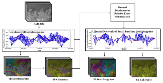
Figure 1.
Flowchart of developed SB interferogram selection algorithm.
3. Case Study Area
Northern Urumqi, China, is located between the Tianshan Mountains and the Gurbantunggut Desert (Figure 2). The average altitude is about 500 m. The area belongs to the middle temperate continental arid region, characterized by long winter and summer seasons [49]. In particular, during winter, from the middle of October to the middle of the following March, the temperature is usually constantly below 0 °C. More than 50 rivers originate in the north of the Tianshan Mountains, supplied by snow cover and melting glaciers. The annual average runoff can reach 82.7947 × 10⁸ m3 [50]. Dense rivers form a large arid alluvial plain in the north of the Tianshan Mountains and gradually develop into typical irrigation agriculture under human activity.
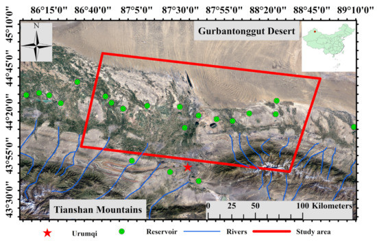
Figure 2.
Google Earth image of the Urumqi region. Study area outlined by red rectangle; rivers shown in blue and reservoirs indicated by green circles. Inset (top right) shows location of study area.
Irrigated agriculture is relatively developed here, one of China’s essential grain production bases. Moreover, since the implementation of the national policy to develop Xinjiang, agricultural land reached 22,330 by 2010, accounting for about 17% of the region’s total land area [51]. The main crops include wheat, corn, melons, fruits and cotton. Agricultural irrigation mainly depends on groundwater and river water. The farmland area is primarily irrigated using river water, whereas areas far from rivers and reservoirs can only rely on groundwater. Many reservoirs are located in the study area, as shown in Figure 2. They store surface water during the rainy season and snowmelt during the spring season. Stored groundwater is then pumped during the summer season to facilitate agricultural irrigation. However, due to the limited surface runoff, groundwater demand has exceeded recharge capacity in agricultural production. In addition, in the permafrost areas, freeze–thaw deformation phenomena occurred.
The average annual temperature of the study area is 6.7–8.9 °C; the average yearly precipitation is 224.28 mm, and the average annual sunshine amounts to 2671.5 h. These conditions create distinctive agricultural resources. There is an excellent climate for agricultural development [52]. However, water consumption for agricultural irrigation is substantial, especially in dry areas. From 1988 to 2015, water consumption for irrigation increased by 256%, and the water consumption of crops increased year by year [53]. The proportion of agricultural water consumption was 92.5% in 2017. Overexploitation of groundwater leads to decreased pore water pressure and land subsidence on irrigated farmland.
4. Experimental Results
4.1. SBAS Ground Deformation Time Series Generation
This research study exploited 102 pieces of Sentinel-1B SAR data collected from 12 April 2017 to 29 October 2020. Table 1 summarizes the main data parameters.

Table 1.
Characteristics of Sentinel-1B SAR data used in this study.
We applied the developed ISA method to the available SAR images to identify an optimized group of SB multi-look interferograms that the conventional SBAS technique has subsequently processed. To this aim, we preliminarily identified a group of “candidate” SB SAR data pairs characterized by the maximum temporal baseline days, and we did not apply any constraint on the maximum perpendicular baseline of the interferograms. Figure 3A shows the distribution of preselected SB interferometric SAR data pairs in the temporal/perpendicular baseline plane. In this domain, the available SAR images are represented by red circles. The arcs connecting pairs of SAR data (drawn in blue) identify the set of candidate SB SAR data pairs. Once identified, a group of 656 SB multi-look interferograms was generated.
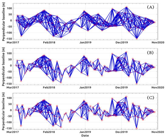
Figure 3.
Distribution of SAR data pairs in a temporal/perpendicular baseline domain. (A) Set of available SB InSAR data pairs estimated by imposing a maximum temporal baseline separation of 90 days. (B) Optimal network of SB interferograms retrieved by applying the proposed InSAR selection algorithm. (C) Reduced network of SB interferograms at boundary condition where one single SB data pair exists that connects the group of interferograms to form a single set of data. Note that (B) and (C) refer to the condition on minimum average spatial coherence of selected interferograms of 0.84 (P1 in Figure 5C) and 0.86 (P2 in Figure 5C).
Precise satellite orbit information and a three-arcsec digital elevation model (DEM) of the area from the Shuttle Radar Topography Mission (SRTM) were used to estimate and remove the topographic phase components. The generated interferograms were independently multi-looked (10 range–2 azimuth looks, respectively) and noise filtered with the use of the Goldstein filter [2] (with alpha = 0.6). Contextually, we also generated the corresponding coherence map for every generated differential SAR interferogram and computed the relevant average coherence value (over the whole imaged area). Figure 4A shows how the average coherence drops as the temporal baseline of the interferograms increases; however, because the S-1 orbital tube is narrow, there is no substantial decoherence strictly related to the perpendicular baselines.
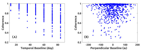
Figure 4.
Scatter plot of average spatial coherence of candidate SB data pairs vs. their (A) temporal and (B) perpendicular baseline.
At this stage, we applied the developed ISA method and identified the optimal set of SB interferograms that minimized the term (see Section 2). We note that, as the applied threshold on the minimum (average) spatial coherence increases, two opposite effects occur: (i) the multi-look interferograms are less affected by decorrelation artifacts, and (ii) the number of interferograms with average coherence greater than drops. These counteracting effects are taken into account by and , respectively. Note that in the limit case, the threshold leads to the formation of two independent sets of SB interferograms, and the condition number becomes infinite as the relative error bound (Equation (6)). In this case, unless there is a substantial time overlap between the two independent subsets of SAR data, the singular value decomposition of matrix B is exploited to solve the least-squares (LS) problem of Equation (1).
Figure 5A,B show the plots of and , respectively, as a function of the average coherence threshold. Figure 5C plots the value of versus the average spatial coherence threshold , highlighting that the optimal condition arises, in our specific case, considering an optimal coherence threshold (P1 in Figure 5C). In this case, an adjusted/optimal network of 421 SB multi-look interferograms is determined. Figure 3B shows the distribution of the selected optimal SB interferometric SAR data pairs in the temporal/perpendicular baseline domain. In Figure 5C, P2 highlights the limit case when only one single interferogram exists to connect two subsets of SB interferograms (e.g., the condition number is maximum but not infinite). This condition corresponds to and to a group of 389 SB differential SAR interferograms in our experiment. Figure 4A shows the distribution of SB interferometric SAR data pairs in the temporal/perpendicular baseline domain for this limit case.
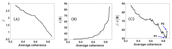
Figure 5.
Plots of (A) , (B) , and (C) vs. the interferometric average spatial coherence threshold.
Some coherence maps are shown in Figure 6. Mainly, Figure 6A,B shows the coherence map of the worst interferogram (i.e., characterized by the minimum average spatial coherence) for the optimal case (P1 in Figure 5C) and the limit case (P2 in Figure 5C), respectively. Furthermore, Figure 6C shows the coherence map of the best interferogram for the whole selected optimal SB interferogram network, and Figure 6D shows the coherence map of the worst candidate, the SB interferogram. The latter does not belong to the set of interferograms used for the SBAS inversion. The master and slave SAR images of the selected SAR data pairs are listed in the caption of Figure 6.
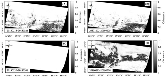
Figure 6.
Spatial coherence maps of four DInSAR SB interferograms. The worst coherence images related to selected optimal set of SB interferograms (P1 condition, Figure 5C) and limit case (P2 condition, Figure 5C), respectively: (A) the coherence map of 18 February 2018 to 26 March 2019 InSAR data pair (average coherence 0.84) and (B) the coherence map of 2 November 2017 to 25 January 2018 (average coherence 0.86). (C) The best coherence map as a whole related to the 20 January 2019 to 1 February 2019 InSAR data pair (average spatial coherence 0.99). (D) The worst coherence map as a whole in the set of candidate SB InSAR data pairs related to the 13 February 2019 to 8 May 2019 InSAR data pair (average spatial coherence 0.28). Although (D) is related to an SB InSAR data pair, it must be discarded to enhance the quality of ground deformation products.
Starting from the optimized set of 421 SB interferometric SAR data pairs shown in Figure 3B, we applied to the relevant multi-look differential interferograms the conventional SBAS-InSAR processing in the implementation provided in the StaMPs software package [18] to generate the ground deformation time series related to stable DS targets. The DS target locations were identified by the phase stability analysis [18] provided in the StaMPs software package. StaMPs implementation processing can be found in [54]. Accordingly, a group of about 3.7 million pixels was selected. Over these pixels, the phase unwrapping operations [55] were implemented to reconstruct the relevant (full) unwrapped phases.
Multi-look unwrapped phases were inverted, pixel by pixel, using the SBAS approach, and the ground deformation time series relevant to the set of coherent SAR pixels were computed. To check the quality of the generated ground displacement time series, we calculated the values of the temporal coherence factor [40], which indirectly measures the probability error of the ground deformation measurements. Temporal coherence has been widely used in SBAS investigations [56,57,58] over the years, and a threshold value of 0.7 is considered legitimate for reliable DInSAR ground deformation products. Large temporal coherence values mean the ground deformation time series are consistent with the measured interferometric phases.
Figure 7 shows the map of temporal coherence. Note that areas with a low temporal coherence value (less than 0.7) are mainly concentrated on the mountains (the lower right corner). Accordingly, these areas were excluded from subsequent analyses. Figure 8A shows the map of ground mean deformation velocity of the investigated area over well-processed radar pixels. Six points, labeled A–E in Figure 8A, were identified in the studied region, whose relevant ground displacement time series are shown in Figure 9. They show that ground deformation time series over the investigated area contain a linear component in time (subsidence), superimposed with a nonlinear seasonal component over an approximately one-year period.
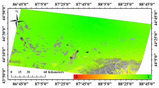
Figure 7.
Map of temporal coherence.
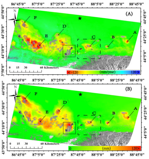
Figure 8.
(A) Mean deformation velocity map of the Urumqi area. (B) Map showing the seasonal deformation amplitude values. Pixels labeled A–F are related to the deformation time series shown in Figure 9. The black star indicates the location of reference point, where deformation is assumed to equal zero. Black dotted lines indicate a rectangular area where a test on ISA effectiveness was carried out. Only SAR pixels with temporal coherence values larger than 0.7 are shown.
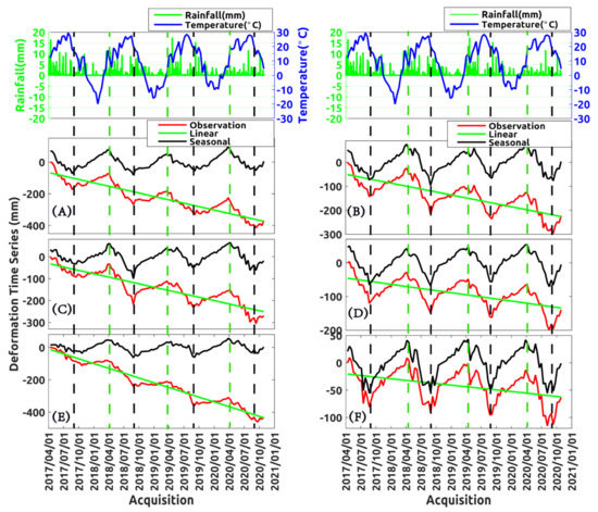
Figure 9.
Deformation, temperature and rainfall time series comparison at six points, A–F (as described in Figure 8). The first line is a rainfall and temperature time series. (A–F) deformation including observation, linear and seasonal deformation time series, respectively. Vertical dotted black and green lines show the inflection points of seasonal term deformation.
To further check the reliability of the obtained SBAS-driven ground deformation results and to prove the effectiveness of the developed ISA, we also generated, using the SBAS technique, the ground deformation time series of the area using the networks of SB interferograms shown in Figure 3A,C, consisting of 656 and 389 SB multi-look interferograms, respectively, the use of which corresponds to the use of “candidate” SB interferograms (A) and the set of interferograms at the limit case. The three generated families of ground displacement time series were jointly analyzed to infer their accuracy. Unfortunately, there is a lack of external, freely available GPS/leveling measurements for validation purposes.
To partially circumvent this problem, we adopted the following strategy. For every family of ground displacement time series, we extracted the relevant spatial low-pass (LP) and high-pass (HP) ground deformation time series (using a moving average window of 10 × 10 pixels). Assuming that the (true) ground deformation is spatially correlated in the averaging box, and considering that the APS is also spatially correlated, we can reasonably assume that the HP components are mainly sensitive to the decorrelation noise and phase unwrapping errors. Thus, an indirect measure of the accuracy of the ground displacement time series could be given by the standard deviation of the HP components in an area of interest. Figure 10 shows a histogram of the HP standard deviation for the three networks of SB interferograms used in this study, as computed over a box centered around the location of point C (see Figure 8B). The values of the average HP standard deviation are 1.56, 1.29 and 1.38 mm for the three SB networks. The result of this experiment shows that the selected optimal SB interferogram network leads to the generation of ground displacement time series that are less noisy.
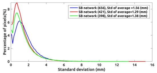
Figure 10.
Histogram of HP standard deviations for three networks of SB interferograms: candidate SB (blue), optimal SB (red), single-subset-limit case (green).
We want to highlight that this experiment only obtains a preliminary assessment of the developed ISA. However, a reasonable quality assessment of the method would require applying it in several different working conditions. However, this is outside the limits of the present investigation and is a matter for future investigation.
4.2. Analysis of Ground Deformation Signals
Let us now focus exclusively on the ground deformation time series related to the optimal SB network of interferograms, shown in Figure 8 and Figure 9. In analyzing these time series, first we discriminated the linear and nonlinear ground deformation components in time. Pixel by pixel, we estimated the linear components by simply fitting the ground displacements with a line. We then subtracted the linear components from the ground deformation time series. We provided the residues, in the LS sense, with a sinusoidal model, Asin(2πt/T), using a least-squares sine fitting algorithm (e.g., [59]), where A and T are the amplitude and period of oscillations. It is worth noting that more sophisticated approaches, such as independent component analysis (ICA) [60,61,62,63], could also be applied to infer the periodical ground deformation components. Figure 8B shows, for every well-processed SAR pixel, the map of amplitudes of periodical (over a period of approximately one year) sinusoidal ground displacements. Of course, this model well fits the ground deformations in the farmland regions, where the deformation signals can be related to groundwater depletion and inflation during a period of one year. Conversely, the quality of fitting deteriorates in other zones of the case study area.
The observed terrain displacement time series were also compared to temperature (blue lines) and rainfall (green histograms). The measured ground displacement time series were decomposed into their main components: long-term linear trend (green lines) and nonlinear seasonal deformation (black lines) time series. The rainfall data and temperature were from [64,65]. The rainfall time series, temperature and deformation time series were mapped to interpret the cause of the deformation pattern. The vertical dotted black and green lines identify the beginning and end of the irrigation periods (approximately from April to October every year), corresponding to the peaks (uplift and subsidence) of seasonal ground displacements.
Let us now focus on the area highlighted by the rectangular black box in Figure 8B. Figure 11 shows a zoomed view of the Bayi Reservoir area. The reservoir was built in 1952 with a catchment area of 15 square kilometers. Its storage capacity reaches 35 million cubic meters for water storage and agricultural irrigation. The west of Bayi Reservoir is a farmland area, and the loss of groundwater causes large-scale land subsidence and threatens the safety of the reservoir. Around the Bayi Reservoir, the linear deformation rate exceeds 40 mm/year (Figure 11B), and the amplitude of seasonal deformation magnitude reaches 120 mm/year (Figure 11C). The deformation pattern includes linear and seasonal deformation. The observed ground deformations represent a threat to the ecological balance and wastewater resources of the area. Figure 11D shows the ground deformation time series of the selected point P. We find that the magnitude of deformation, including seasonal and linear deformation, is low in the non-farmland area. Conversely, in the farmland area (between Qinggeda Lake and Bayi Reservoir), seasonal deformation is high.
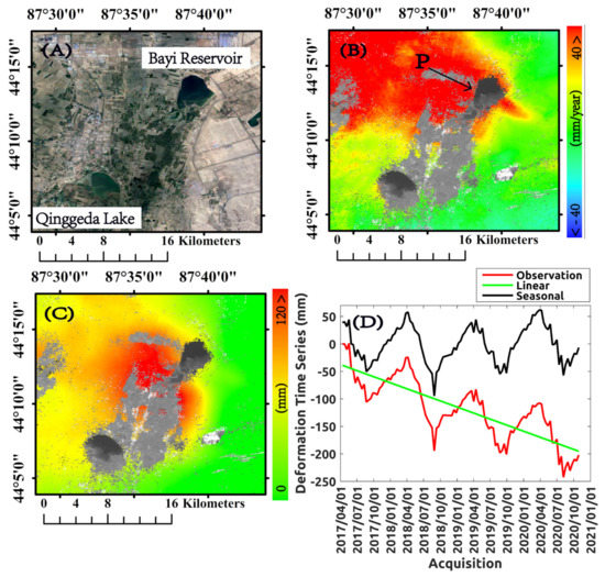
Figure 11.
(A) Zoomed view of the optical image shown in Figure 8, corresponding to Bayi Reservoir and Qinggeda Lake. (B) Mean deformation velocity map. (C) Map of seasonal deformation amplitude values. (D) Plot of the ground deformation time series related to point P, highlighted by a black arrow in (B).
5. Discussion
In this section, we discuss our research findings by focusing on the proposed ISA method and the primary outcomes of the SBAS investigation in the considered case study area.
One of the main achievements of our investigation was that we developed and preliminarily checked the potential of a novel strategy to automatically select small baseline interferometric SAR data pairs that the SBAS DInSAR technique can use. The selected SB network is the result of a compromise, considering both the effects of the average coherence of the SB interferograms and the connectivity of the resulting SB network. Too few interferograms might lead to SB networks that are less redundant. Thus, even minor errors in single multi-look interferograms, such as phase unwrapping errors, can severely corrupt the generated ground deformation time series. On the other hand, too many interferograms might lead to noisier ground deformation time series due to the presence of interferograms that are more decorrelated, even using SAR data pairs with small temporal and perpendicular baseline separations. Phase decorrelation also magnifies the phase unwrapping errors that can propagate from noisy interferograms to good interferograms due to the SB network redundancy. Therefore, it is mandatory to find a proper balance between these two distinctive effects. The proposed ISA aims to find such a balance condition. The optimal set of interferograms can be used to investigate surface deformations in large-scale areas rapidly to obtain ground deformation time series.
The results of the experiments shown in Section 4.1 (Figure 10) demonstrate that the accuracy of SBAS ground deformation time series improves when the optimal network of SB interferograms is used. We note that some assumptions were made to obtain these results; specifically, we assumed that ground deformations are spatially correlated. Certainly, further extended analyses are required to quantitatively assess the performance of the developed ISA method.
With the results obtained from the SBAS analyses performed in the selected case study area, we derived ground deformation time series. We inferred the sources of ground deformations, discriminating long-term zone deformations (linear trend) from seasonal deformations related to one-year irrigation and the freeze–thaw cycles of the frozen area under investigation. In terms of water consumption, the study area is located between deserts in the north and the Tianshan Mountain in the south.
The observed land subsidence in the farmland areas is related to irrigation methods and facilities related to groundwater recharge and consumption, as shown in Figure 8B, where the amplitude of seasonal ground displacements is shown. Notably, we noticed that these seasonal changes are superimposed over a general trend of subsidence of irrigated land that has evolved over recent years (2017 to 2020). The small-scale land subsidence caused by overexploitation of groundwater in the Northern Urumqi region has been investigated [66].
The analysis of the plots shown in Figure 11 shows that the deformation time series are moderately correlated to temperature variations. Note that in the study areas, the temperature difference in a year is enormous; the highest temperature is 41 °C and the lowest is −28 °C. In these areas, instead of permafrost, temperature changes can lead to freezing and thawing. Moreover, our results suggest that the observed ground deformation is mainly related to the yearly farmland irrigation cycle, which usually starts in March/April and ends in October. This is in agreement with what is shown by the nonlinear deformation time series of points A-F depicted in Figure 11. Of course, there is a correlation between seasonal temperature variations and irrigation cycles. This is the reason for the inferred moderate correlation between ground displacement and temperature. Our results are in general agreement with the outcomes of a research study [66] that investigated small-scale ground deformations linked to irrigation in the Northern Urumqi region by using first-generation ENVISAT/ASAR images collected from 2003 to 2009.
It is documented that rainfall and temperature have little influence on the groundwater level changes in this area [67]. Accordingly, most of these changes can be related to human activities and particularly to the irrigation of farmland. Indeed, the starting and stopping of agricultural irrigation strictly regulates groundwater depth [67]. Mainly during the agricultural irrigation period, subsidence deformation is caused by the overexploitation of groundwater. In the period when irrigation activities are stopped, uplift deformation depends on the recharge of groundwater [66]. These seasonal groundwater level changes thus have an impact on the observed nonlinear ground deformation, as shown in Figure 11, where the dotted green and black lines highlight the beginning and end of the irrigation period. As a final remark, from our data analysis, we also underline that in this area, the ground displacements driven by irrigation are more significant than those due to the expansion and contraction of the terrain caused by freezing and thawing, which represent the second-order factor that is superimposed on the observed nonlinear ground deformations.
6. Conclusions
In this paper, we propose a novel strategy for selecting an adjusted network of SB interferograms to be subsequently used by the conventional SBAS technique to obtain ground deformation time series. The developed interferogram selection method aims to minimize the relative error of mean ground displacement velocity measurements based on the primary outcomes of recent theoretical studies. Further efforts are still required to generalize the method to consider other quality parameters of the selected interferograms and take into account the effects of phase unwrapping errors and APS artifacts in order to select the optimal set of SB interferograms. The developed ISA was first tested considering Sentinel-1B SAR data acquired over the farmland area of the Northern Urumqi region, China. Of course, evaluating the capabilities of the developed method would require applying it to several case study areas. However, this is a matter for future investigation. Concerning the results obtained by applying this method to the investigated region, we note that SBAS analysis showed that the primary source of the observed ground deformations is primarily related to the overexploitation of groundwater for farmland irrigation. The groundwater in arid areas is of great significance to maintain the stability of the ecosystem. Thus, in areas where water resources are scarce, to ensure the healthy development of agriculture, it is very important to change the traditional irrigation methods and improve the utilization rate of water resources.
Author Contributions
B.W. and A.P. designed the experiments. B.W. performed the experiments and produced the results. B.W., Q.Z., A.P. and P.M. drafted and finalized the manuscript. Z.L., C.Z., W.Z., C.Y. and J.Z. contributed to the discussion of the results. All authors have read and agreed to the published version of the manuscript.
Funding
This research was funded by the National Key R&D Program of China (nos. 2018YFC1505102 and 2018YFC1504805), the Natural Science Foundation of China (grant nos. 41731066, 41874005, and 41929001) and Fundamental Research Funds for the Central Universities (grant nos. 300102269303 and 300102269719).
Institutional Review Board Statement
The study did not involve humans or animals.
Informed Consent Statement
The study did not involve humans.
Data Availability Statement
The study did not involve humans.
Acknowledgments
We are grateful to the European Space Agency for providing Sentinel-1B data.
Conflicts of Interest
The authors declare no conflict of interest.
References
- Massonnet, D.; Rossi, M.; Carmona, C.; Adragna, F.; Peltzer, G.; Feigl, K.; Rabaute, T. The displacement field of the Landers earthquake mapped by radar interferometry. Nature 1993, 364, 138–142. [Google Scholar] [CrossRef]
- Goldstein, R.M.; Werner, C.L. Radar interferogram filtering for geophysical applications. Geophys. Res. Lett. 1998, 25, 4035–4038. [Google Scholar] [CrossRef]
- Bürgmann, R.; Rosen, P.A.; Fielding, E.J. Synthetic Aperture Radar Interferometry to Measure Earth’s Surface Topography and Its Deformation. Annu. Rev. Earth Planet. Sci. 2000, 28, 169–209. [Google Scholar] [CrossRef]
- Rosen, P.A.; Hensley, S.; Joughin, I.R.; Li, F.K.; Madsen, S.N.; Rodriguez, E.; Goldstein, R.M. Synthetic aperture radar interferometry. Proc. IEEE 2002, 88, 333–382. [Google Scholar] [CrossRef]
- Ferretti, A.; Prati, C.; Rocca, F. Permanent scatterers in SAR interferometry. IEEE Trans. Geosci. Remote Sens. 2001, 39, 8–20. [Google Scholar] [CrossRef]
- Werner, C.; Wegmuller, U.; Strozzi, T.; Wiesmann, A. Interferometric point target analysis for deformation mapping. In Proceedings of the International Geoscience and Remote Sensing Symposium (IGARSS), Toulouse, France, 21–25 July 2003; Volume 7, pp. 4362–4364. [Google Scholar]
- Hooper, A.; Zebker, H.; Segall, P.; Kampes, B. A new method for measuring deformation on volcanoes and other natural terrains using InSAR persistent scatterers. Geophys. Res. Lett. 2004, 31. [Google Scholar] [CrossRef]
- Kampes, B. Radar Interferometry: Persistent Scatterer Technique; Springer: Dordrecht, The Netherlands, 2006. [Google Scholar]
- Berardino, P.; Fornaro, G.; Lanari, R.; Sansosti, E. A new algorithm for surface deformation monitoring based on small baseline differential SAR interferograms. IEEE Trans. Geosci. Remote Sens. 2002, 40, 2375–2383. [Google Scholar] [CrossRef]
- Zebker, H.A.; Villasenor, J. Decorrelation in interferometric radar echoes. IEEE Trans. Geosci. Remote Sens. 1992, 30, 950–959. [Google Scholar] [CrossRef]
- Pepe, A.; Ortiz, A.B.; Lundgren, P.R.; Rosen, P.A.; Lanari, R. The Stripmap–ScanSAR SBAS Approach to Fill Gaps in Stripmap Deformation Time Series with ScanSAR Data. IEEE Trans. Geosci. Remote Sens. 2011, 49, 4788–4804. [Google Scholar] [CrossRef]
- Fialko, Y. Interseismic strain accumulation and the earthquake potential on the southern San Andreas fault system. Nature 2006, 441, 968–971. [Google Scholar] [CrossRef]
- Ferretti, A.; Fumagalli, A.; Novali, F.; Prati, C.P.; Rocca, F.; Rucci, A. A New Algorithm for Processing Interferometric Data-Stacks: SqueeSAR. IEEE Trans. Geosci. Remote Sens. 2011, 49, 3460–3470. [Google Scholar] [CrossRef]
- Pepe, A.; Mastro, P.; Jones, C.E. Adaptive Multilooking of Multitemporal Differential SAR Interferometric Data Stack Using Directional Statistics. IEEE Trans. Geosci. Remote Sens. 2020, 99, 1–16. [Google Scholar] [CrossRef]
- Parizzi, A.; Brcic, R. Adaptive InSAR Stack Multilooking Exploiting Amplitude Statistics: A Comparison Between Different Techniques and Practical Results. IEEE Geosci. Remote Sens. Lett. 2010, 8, 441–445. [Google Scholar] [CrossRef]
- Wang, Y.; Deng, Y.; Fei, W.; Wang, R.; Song, H.; Wang, J.; Li, N. Modified Statistically Homogeneous Pixels’ Selection with Multitemporal SAR Images. IEEE Geosci. Remote Sens. Lett. 2016, 13, 1–5. [Google Scholar] [CrossRef]
- Shi, G.; Ma, P.; Lin, H.; Huang, B.; Zhang, B.; Liu, Y. Potential of Using Phase Correlation in Distributed Scatterer InSAR Applied to Build Scenarios. Remote Sens. 2020, 12, 686. [Google Scholar] [CrossRef]
- Hooper, A. A multi-temporal InSAR method incorporating both persistent scatterer and small baseline approaches. Geophys. Res. Lett. 2008, 35, 96–106. [Google Scholar] [CrossRef]
- Osmanoğlu, B.; Sunar, F.; Wdowinski, S.; Cabral-Cano, E. Time series analysis of InSAR data: Methods and trends. ISPRS J. Photogramm. Remote Sens. 2016, 115, 90–102. [Google Scholar] [CrossRef]
- Minh, D.H.T.; Hanssen, R.; Rocca, F. Radar Interferometry: 20 Years of Development in Time Series Techniques and Future Perspectives. Remote Sens. 2020, 12, 1364. [Google Scholar] [CrossRef]
- Montalti, R.; Solari, L.; Bianchini, S.; del Soldato, M.; Raspini, F.; Casagli, N. A Sentinel-1-based clustering analysis for geo-hazards mitigation at regional scale: A case study in Central Italy. Geomat. Nat. Hazards Risk 2019, 10, 2257–2275. [Google Scholar] [CrossRef]
- Schaefer, L.N.; di Traglia, F.; Chaussard, E.; Lu, Z.; Nolesini, T.; Casagli, N. Monitoring volcano slope instability with Synthetic Aperture Radar: A review and new data from Pacaya (Guatemala) and Stromboli (Italy) volcanoes. Earth Sci. Rev. 2019, 192, 236–257. [Google Scholar] [CrossRef]
- Castellazzi, P.; Longuevergne, L.; Martel, R.; Rivera, A.; Brouard, C.; Chaussard, E. Quantitative mapping of groundwater depletion at the water management scale using a combined GRACE/InSAR approach. Remote Sens. Environ. 2017, 205, 408–418. [Google Scholar] [CrossRef]
- Liu, L.; Zhang, T.; Wahr, J. InSAR measurements of surface deformation over permafrost on the North Slope of Alaska. J. Geophys. Res. Space Phys. 2010, 115, F3. [Google Scholar] [CrossRef]
- Short, N.; Brisco, B.; Couture, N.; Pollard, W.; Murnaghan, K.; Budkewitsch, P. A comparison of TerraSAR-X, Radarsat-2 and ALOS-Palsar interferometry for monitoring permafrost environments, case study from Herschel Island, Canada. Remote Sens. Environ. 2011, 115, 3491–3506. [Google Scholar] [CrossRef]
- Daout, S.; Doin, M.P.; Peltzer, G.; Socquet, A.; Lasserre, C. Large-scale InSAR monitoring of permafrost freeze-thaw cycles on the Tibetan Plateau. Geophys. Res. Lett. 2017, 44, 901–909. [Google Scholar] [CrossRef]
- Chen, J.; Liu, L.; Zhang, T.; Cao, B.; Lin, H. Using Persistent Scatterer Interferometry to Map and Quantify Permafrost Thaw Subsidence: A Case Study of Eboling Mountain on the Qinghai-Tibet Plateau. J. Geophys. Res. Earth Surf. 2018, 123, 2663–2676. [Google Scholar] [CrossRef]
- Wang, C.; Zhang, Z.; Zhang, H.; Wu, Q.; Zhang, B.; Tang, Y. Seasonal deformation features on Qinghai-Tibet railway observed using time-series InSAR technique with high-resolution TerraSAR-X images. Remote Sens. Lett. 2017, 8, 1–10. [Google Scholar] [CrossRef]
- Dai, K.; Liu, G.; Li, Z.; Ma, D.; Wang, X.; Zhang, B.; Tang, J.; Li, G. Monitoring Highway Stability in Permafrost Regions with X-band Temporary Scatterers ing InSAR. Sensors 2018, 18, 1876. [Google Scholar] [CrossRef] [PubMed]
- Rudy, A.C.; Lamoureux, S.F.; Treitz, P.; Short, N.; Brisco, B. Seasonal and multi-year surface displacements measured by DInSAR in a High Arctic permafrost environment. Int. J. Appl. Earth Obs. Geoinf. 2018, 64, 51–61. [Google Scholar] [CrossRef]
- Molan, Y.E.; Kim, J.-W.; Lu, Z.; Wylie, B.; Zhu, Z. Modeling Wildfire-Induced Permafrost Deformation in an Alaskan Boreal Forest Using InSAR Observations. Remote Sens. 2018, 10, 405. [Google Scholar] [CrossRef]
- Wang, S.; Xu, B.; Shan, W.; Shi, J.; Li, Z.; Feng, G. Monitoring the Degradation of Island Permafrost Using Time-Series InSAR Technique: A Case Study of Heihe, China. Sensors 2019, 19, 1364. [Google Scholar] [CrossRef]
- Strozzi, T.; Antonova, S.; Günther, F.; Mätzler, E.; Vieira, G.; Wegmüller, U.; Westermann, S.; Bartsch, A. Sentinel-1 SAR Interferometry for Surface Deformation Monitoring in Low-Land Permafrost Areas. Remote Sens. 2018, 10, 1360. [Google Scholar] [CrossRef]
- Wang, C.; Zhang, Z.; Zhang, H.; Zhang, B.; Tang, Y.; Wu, Q. Active layer thickness retrieval of Qinghai-Tibet permafrost using the TerraSAR-X InSAR technique. IEEE J. Sel. Top. Appl. Earth Obs. Remote Sens. 2018, 11, 4403–4413. [Google Scholar] [CrossRef]
- Widhalm, B.; Bartsch, A.; Leibman, M.; Khomutov, A. Active-layer thickness estimation from X-band SAR backscatter intensity. Cryosphere 2017, 11, 483–496. [Google Scholar] [CrossRef]
- Chen, J.; Wu, Y.; O’Connor, M.; Cardenas, M.B.; Schaefer, K.; Michaelides, R.; Kling, G. Active layer freeze-thaw and water storage dynamics in permafrost environments inferred from InSAR. Remote Sens. Environ. 2020, 248, 112007. [Google Scholar] [CrossRef]
- Refice, A.; Bovenga, F.; Nutricato, R. MST-based stepwise connection strategies for multipass Radar data, with application to coregistration and equalization. IEEE Trans. Geosci. Remote Sens. 2006, 44, 2029–2040. [Google Scholar] [CrossRef]
- Perissin, D.; Wang, T. Repeat-Pass SAR Interferometry with Partially Coherent Targets. IEEE Trans. Geosci. Remote Sens. 2011, 50, 271–280. [Google Scholar] [CrossRef]
- Pepe, A.; Yang, Y.; Manzo, M.; Lanari, R. Improved EMCF-SBAS Processing Chain Based on Advanced Techniques for the Noise-Filtering and Selection of Small Baseline Multi-Look DInSAR Interferograms. IEEE Trans. Geosci. Remote Sens. 2015, 53, 4394–4417. [Google Scholar] [CrossRef]
- Pepe, A.; Lanari, R. On the Extension of the Minimum Cost Flow Algorithm for Phase Unwrapping of Multitemporal Differential SAR Interferograms. IEEE Trans. Geosci. Remote Sens. 2006, 44, 2374–2383. [Google Scholar] [CrossRef]
- Duan, M.; Xu, B.; Li, Z.W.; Wu, W.H.; Wei, J.C.; Cao, Y.M.; Liu, J.H. Adaptively Selecting Interferograms for SBAS-InSAR Based on Graph Theory and Turbulence Atmosphere. IEEE Access 2020, 99, 1. [Google Scholar]
- Wu, H.A.; Zhang, Y.; Kang, Y.; Lu, Z.; Cheng, X. Semi-automatic selection of optimum image pairs based on the interferometric coherence for time series SAR interferometry. Remote Sens. Lett. 2019, 10, 1105–1112. [Google Scholar] [CrossRef]
- Zhao, B.C.; Wang, Q.B.; Zhang, Q.; Zhu, W.Q. Batch filtering of multi-baseline SAR interferograms. In 2017 SAR in Big Data Era: Models, Methods and Applications (BIGSARDATA); IEEE: Beijing, China, 2017; pp. 1–4. [Google Scholar]
- Pepe, A. Multi-Temporal Small Baseline Interferometric SAR Algorithms: Error Budget and Theoretical Performance. Remote Sens. 2021, 13, 557. [Google Scholar] [CrossRef]
- Vaccaro, R.; Kot, A. A Perturbation Theory for the Analysis of SVD-Based Algorithms. In Proceedings of the ICASSP ’87 IEEE International Conference on Acoustics, Speech, and Signal Processing, Dallas, TX, USA, 6–9 April 1987; 12, pp. 1613–1616. [Google Scholar]
- Wei, M. The perturbation of consistent least squares problems. Linear Algebra Appl. 1989, 112, 231–245. [Google Scholar] [CrossRef][Green Version]
- Demmel, J.W. Applied Numerical Linear Algebra; SIAM: Philadelphia, PA, USA, 1997; ISBN 978-0-89871-389-3. [Google Scholar]
- Bamler, R.; Hartl, P. Synthetic aperture radar interferometry. Inverse Probl. 1998, 14, R1–R54. [Google Scholar] [CrossRef]
- Climatic characteristics. Available online: http://www.urumqi.gov.cn/zjsf2/zrdl/185.htm (accessed on 5 May 2021).
- Aziguli, Y. Discussion on Xinjiang water utilization and agricultural sustainable development. Gansu Nongye 2007, 1, 40–41. (In Chinese) [Google Scholar]
- Xu, L.P.; Guo, P.; Liu, L.; Wang, L. Analysis of the spatiotemporal features of land use and land degradation in the northern pied-mont area of the Tianshan Mountain. Res. Soil Water Conserv. 2014, 21, 316–321. (In Chinese) [Google Scholar]
- Chen, H.X.; Li, J.Y.; Yang, D.G.; Li, X.H.; Cai, T.Y.; Xia, F.G. Spatial distribution of agricultural production from perspective of water footprint: A case study of north-piedmont major agriculture production regions of Tianshan Mountains, Xinjiang. J. Univ. Chin. Acad. Sci. 2021, 38, 240–251. (In Chinese) [Google Scholar]
- Zhang, P.; Long, A.H.; Hai, Y.; Deng, X.Y.; Wang, J.; Liu, J.; Li, Y. Spatiotemporal variations and driving forces of agricultural water consumption in Xinjiang during 1988—2015: Based on statistical analysis of crop water footprint. J. Glaciol. Geocryol. 2021, 43, 242–253. (In Chinese) [Google Scholar]
- StaMPS. Available online: http://homepages.see.leeds.ac.uk/~earahoo/stamps/ (accessed on 5 May 2021).
- Hooper, A.; Zebker, H.A. Phase unwrapping in three dimensions with application to InSAR time series. J. Opt. Soc. Am. A 2007, 24, 2737–2747. [Google Scholar] [CrossRef]
- Manzo, M.; Fialko, Y.; Casu, F.; Pepe, A.; Lanari, R. A Quantitative Assessment of DInSAR Measurements of Interseismic Deformation: The Southern San Andreas Fault Case Study. Pure Appl. Geophys. PAGEOPH 2012, 169, 1463–1482. [Google Scholar] [CrossRef]
- De Novellis, V.; Carlino, S.; Castaldo, R.; Tramelli, A.; de Luca, C.; Pino, N.A.; Pepe, S.; Convertito, V.; Zinno, I.; de Martino, P.; et al. The 21 August 2017 Ischia (Italy) Earthquake Source Model Inferred from Seismological, GPS, and DInSAR Measurements. Geophys. Res. Lett. 2018, 45, 2193–2202. [Google Scholar] [CrossRef]
- Ruch, J.; Pepe, S.; Casu, F.; Acocella, V.; Neri, M.; Solaro, G.; Sansosti, E. How do volcanic rift zones relate to flank instability? Evidence from collapsing rifts at Etna. Geophys. Res. Lett. 2012, 39, L20311. [Google Scholar] [CrossRef]
- Renczes, I.B.; Kollar, I.; Daboczi, T. Efficient Implementation of Least Squares Sine Fitting Algorithms. IEEE Trans. Instrum. Meas. 2016, 65, 2717–2724. [Google Scholar] [CrossRef]
- Ebmeier, S.K. Application of independent component analysis to multitemporal InSAR data with volcanic case studies. J. Geophys. Res. Solid Earth 2016, 121, 8970–8986. [Google Scholar] [CrossRef]
- Cohen-Waeber, J.; Bürgmann, R.; Chaussard, E.; Giannico, C.; Ferretti, A. Spatiotemporal Patterns of Precipitation-Modulated Landslide Deformation from Independent Component Analysis of InSAR Time Series. Geophys. Res. Lett. 2018, 45, 1878–1887. [Google Scholar] [CrossRef]
- Gaddes, M.E.; Hooper, A.; Bagnardi, M.; Inman, H.; Albino, F. Blind Signal Separation Methods for InSAR: The Potential to Automatically Detect and Monitor Signals of Volcanic Deformation. J. Geophys. Res. Solid Earth 2018, 123, 10–226. [Google Scholar] [CrossRef]
- Chaussard, E.; Farr, T.G. A New Method for Isolating Elastic from Inelastic Deformation in Aquifer Systems: Application to the San Joaquin Valley, CA. Geophys. Res. Lett. 2019, 46, 10800–10809. [Google Scholar] [CrossRef]
- Historical weather in Urumqi. Available online: http://lishi.tianqi.com/wulumuqi/index.html. (accessed on 5 May 2021).
- Global Precipitation Measurements. Available online: https://gpm.nasa.gov/data/directory. (accessed on 5 May 2021).
- Wang, H.Y.; Feng, G.C.; Lu, M.; Tian, J.; Xiong, Z.Q. The characteristics and evolution of surface deformation induced by agricultural irrigation in the Junggar Basin from the perspective of InSAR. J. Remote Sens. 2020, 24, 1234–1242. (In Chinese) [Google Scholar]
- Lei, L.; Zhao, Z.Y.; Meng, M.; Qiao, M.; Zhou, S.B. Study on Dynamic Change of Groundwater Depth in a Newly Reclaimed Oasis in Northwestern Marginal Zone of the Junggar Basin. Arid Zone Res. 2011, 28, 751–755. (In Chinese) [Google Scholar]
Publisher’s Note: MDPI stays neutral with regard to jurisdictional claims in published maps and institutional affiliations. |
© 2021 by the authors. Licensee MDPI, Basel, Switzerland. This article is an open access article distributed under the terms and conditions of the Creative Commons Attribution (CC BY) license (https://creativecommons.org/licenses/by/4.0/).