
An Improved Back-Projection Algorithm for GNSS-R BSAR Imaging Based on CPU and GPU Platform

Abstract
1. Introduction
- Using Fast Back Projection Algorithm (FBPA) for GNSS-R BSAR imaging has the advantage of reducing the computational cost, but it will reduce the quality of the imaging [29].
2. Materials
3. Methods
3.1. Review on BPA
3.2. Data Pre-Processing
3.3. Theoretical Analysis of the Improved BPA
3.3.1. Range Compression
3.3.2. Back Projection and Phase Compensation
3.3.3. Azimuth Compression
3.4. Parallelized BPA on GPU
3.4.1. Parallelized Range Compression on GPU
- (1)
- and are determined according to the size of one segment data, where and are the number of range and azimuth samples, respectively. The memory of CPU and GPU are requested for the host for the corresponding data, respectively, and the data are transferred from the memory of the CPU to the memory of the GPU.
- (2)
- The cuFFT library function of CUDA is used to complete the FFT of the reference signal and echo signal, respectively.
- (3)
- The kernel function of parallel complex multiplication of reference signal complex conjugate matrix and echo signal matrix in the frequency domain is designed. Threads are allocated to compressed data based on range gate, and kernel function is called to complete parallel complex multiplication.
- (4)
- Use the cuFFT library function to develop the IFFT solution to convert the range compressed data into the time domain, generate correlation values that match the slant range.
- (5)
- Repeat the steps (1)–(4) until all echo data are processed.
3.4.2. Parallelized Back Projection on GPU
- (1)
- Calculate the delay by constructing a kernel function to allocate threads to each pixel at a range code.
- (2)
- According to the delay of each pixel , the information in the corresponding range gate in the range compression is selected, and the compensation factor is constructed according to the slant range information and the phase difference value.
- (3)
- Phase compensation is performed by complex multiplication of the range compression data for that pixel point with the compensation factor in the time domain. The kernel function will be invoked tens of thousands of times to complete the complex multiplication and complex addition processing.
- (4)
- The data from each azimuthal moment is coherently summed to generate the subimage .
- (5)
- Repeat steps (1)–(4) until all echo data are processed.
4. Results
- (1)
- C++ as a reference compiled procedural language using the Faster Fourier Transform in the West (FFTW) library version 3.3.5.
- (2)
- CUDA 10 with the cuFFT and NPP included libraries.
4.1. Simulation
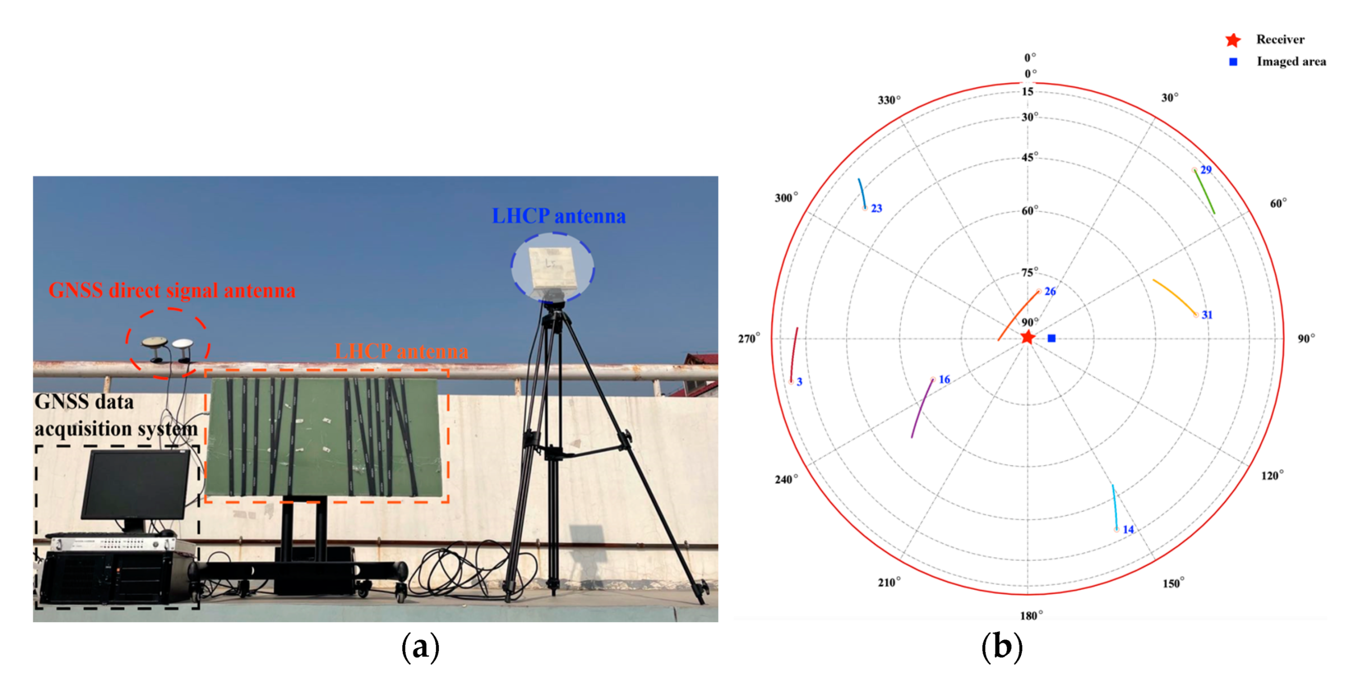
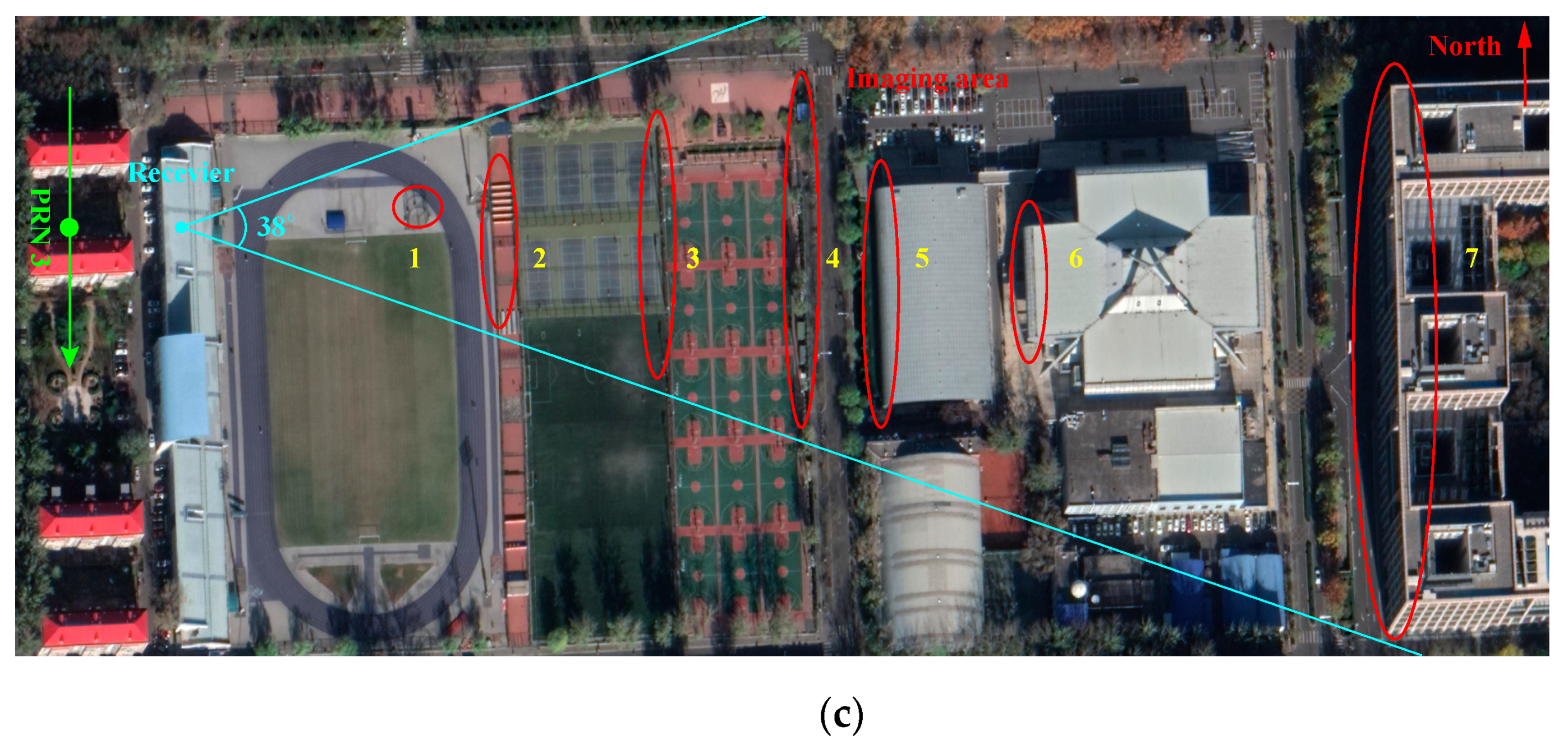
4.2. Experiments
5. Discussion
- (1)
- The geometry of GNSS-R BSAR is complex. The BPA can focus the echo data without the influence of geometry, while the frequency domain algorithms are greatly affected by the geometric structure [28]. Especially in the multisatellite fusion or multistation fusion mode [19,23], more complex geometry will lead to most of the frequency domain algorithm, which is no longer applicable.
- (2)
- The frequency domain algorithms rely on the accuracy of the equivalent squint model and cannot achieve a long-time synthetic aperture [41]. However, increasing the synthetic aperture time can not only improve the azimuth resolution and signal-to-noise ratio but also improve the characteristic information of the target in the imaged area [24]. Especially in one station fixed mode, the synthetic aperture time can reach thousands of seconds. The BPA algorithm is not affected by the synthetic aperture time.
6. Conclusions
Author Contributions
Funding
Institutional Review Board Statement
Informed Consent Statement
Data Availability Statement
Acknowledgments
Conflicts of Interest
References
- Hall, C.D.; Cordey, R.A. Multistatic Scatterometry. In Proceedings of the International Geoscience and Remote Sensing Symposium, Edinburgh, UK, 12–16 September 1988; pp. 561–562. [Google Scholar]
- Martin-neira, M. A Passive Reflectometry and Interferometry System (PARIS): Application to ocean altimetry. ESA J. 1993, 17, 331–355. [Google Scholar]
- Foti, G.; Gommenginger, C.; Jales, P.; Unwin, M.; Shaw, A.; Robertson, C.; Rosello, J. Spaceborne GNSS-Reflectometry for ocean winds: First results from the UK TechDemoSat-1 mission: Spaceborne GNSS-R: First TDS-1 results. Geophys. Res. Lett. 2015, 42. [Google Scholar] [CrossRef]
- Clarizia, M.P.; Ruf, C.S.; Jales, P.; Gommenginger, C. Spaceborne GNSS-R Minimum Variance Wind Speed Estimator. IEEE Geosci. Remote Sens. 2014, 52, 6829–6843. [Google Scholar] [CrossRef]
- Wang, F.; Yang, D.; Yang, L. Feasibility of Wind Direction Observation Using Low-Altitude Global Navigation Satellite System-Reflectometry. IEEE J. Sel. Top. Appl. Earth Obs. Remote Sens. 2018, 11, 5063–5075. [Google Scholar] [CrossRef]
- Li, W.; Cardellach, E.; Fabra, F.; Ribó, S.; Rius, A. Effects of PRN-Dependent ACF Deviations on GNSS-R Wind Speed Retrieval. IEEE Geosci. Remote Sens. Lett. 2019, 16, 327–331. [Google Scholar] [CrossRef]
- Rius, A.; Nogués-Correig, O.; Ribó, S.; Cardellach, E.; Oliveras, S.; Valencia, E.; Park, H.; Tarongí, J.M.; Camps, A.; van der Marel, H.; et al. Altimetry with GNSS-R interferometry: First proof of concept experiment. GPS Solut. 2012, 16, 231–241. [Google Scholar] [CrossRef]
- Cardellach, E.; Rius, A.; Martín-Neira, M.; Fabra, F.; Nogués-Correig, O.; Ribó, S.; Kainulainen, J.; Camps, A.; Addio, S.D. Consolidating the Precision of Interferometric GNSS-R Ocean Altimetry Using Airborne Experimental Data. IEEE Geosci. Remote Sens. 2014, 52, 4992–5004. [Google Scholar] [CrossRef]
- Li, W.; Yang, D.; Addio, S.D.; Martín-Neira, M. Partial Interferometric Processing of Reflected GNSS Signals for Ocean Altimetry. IEEE Geosci. Remote Sens. Lett. 2014, 11, 1509–1513. [Google Scholar] [CrossRef]
- Lowe, S.T.; LaBrecque, J.L.; Zuffada, C.; Romans, L.J.; Young, L.E.; Hajj, G.A. First spaceborne observation of an Earth-reflected GPS signal. Radio Sci. 2002, 37, 1–28. [Google Scholar] [CrossRef]
- Rodriguez-Alvarez, N.; Camps, A.; Vall-llossera, M.; Bosch-Lluis, X.; Monerris, A.; Ramos-Perez, I.; Valencia, E.; Marchan-Hernandez, J.F.; Martinez-Fernandez, J.; Baroncini-Turricchia, G.; et al. Land Geophysical Parameters Retrieval Using the Interference Pattern GNSS-R Technique. IEEE Trans. Geosci. Remote Sens. 2011, 49, 71–84. [Google Scholar] [CrossRef]
- Rodriguez Alvarez, N.; Bosch, X.; Camps, A.; Vall-llossera, M.; Valencia, E.; Marchan, J.; Ramos-Perez, I. Soil Moisture Retrieval Using GNSS-R Techniques: Experimental Results over a Bare Soil Field. IEEE Trans. Geosci. Remote Sens. 2009, 47, 3616–3624. [Google Scholar] [CrossRef]
- Egido, A.; Paloscia, S.; Motte, E.; Guerriero, L.; Pierdicca, N.; Caparrini, M.; Santi, E.; Fontanelli, G.; Floury, N. Airborne GNSS-R Polarimetric Measurements for Soil Moisture and Above-Ground Biomass Estimation. IEEE J. Sel. Top. Appl. Earth Obs. Remote Sens. 2014, 7, 1522–1532. [Google Scholar] [CrossRef]
- Ferrazzoli, P.; Guerriero, L.; Pierdicca, N.; Rahmoune, R. Forest biomass monitoring with GNSS-R: Theoretical simulations. Adv. Space Res. 2011, 47, 1823–1832. [Google Scholar] [CrossRef]
- Wu, X.; Ma, W.; Xia, J.; Bai, W.; Jin, S.; Calabia, A. Spaceborne GNSS-R Soil Moisture Retrieval: Status, Development Opportunities, and Challenges. Remote Sens. 2021, 13, 45. [Google Scholar] [CrossRef]
- Carreno-Luengo, H.; Luzi, G.; Crosetto, M. Above-Ground Biomass Retrieval over Tropical Forests: A Novel GNSS-R Approach with CyGNSS. Remote Sens. 2020, 12, 1368. [Google Scholar] [CrossRef]
- Li, C.; Huang, W. Sea surface oil slick detection from GNSS-R Delay-Doppler Maps using the spatial integration approach. In Proceedings of the 2013 IEEE Radar Conference (RadarCon13), Ottawa, ON, Canada, 29 April–3 May 2013; pp. 1–6. [Google Scholar]
- Gao, H.; Yang, D.; Wang, F.; Wang, Q.; Li, X. Retrieval of Ocean Wind Speed Using Airborne Reflected GNSS Signals. IEEE Access 2019, 7, 71986–71998. [Google Scholar] [CrossRef]
- Antoniou, M.; Cherniakov, M. GNSS-based bistatic SAR: A signal processing view. EURASIP J. Adv. Signal Process. 2013, 2013. [Google Scholar] [CrossRef]
- Zhou, X.; Wang, P.; Chen, J.; Men, Z.; Liu, W.; Zeng, H. A Modified Radon Fourier Transform for GNSS-Based Bistatic Radar Target Detection. IEEE Geosci. Remote Sens. Lett. 2020, 1–5. [Google Scholar] [CrossRef]
- Liu, F.; Fan, X.; Zhang, T.; Liu, Q. GNSS-Based SAR Interferometry for 3-D Deformation Retrieval: Algorithms and Feasibility Study. IEEE Geosci. Remote Sens. 2018, 56, 5736–5748. [Google Scholar] [CrossRef]
- Liu, F.; Antoniou, M.; Zeng, Z.; Cherniakov, M. Coherent Change Detection Using Passive GNSS-Based BSAR: Experimental Proof of Concept. IEEE Trans. Geosci. Remote Sens. 2013, 51, 4544–4555. [Google Scholar] [CrossRef]
- Wu, S.; Yang, D.; Zhu, Y.; Wang, F. Improved GNSS-Based Bistatic SAR Using Multi-Satellites Fusion: Analysis and Experimental Demonstration. Sensors 2020, 20, 7119. [Google Scholar] [CrossRef]
- Liu, F.; Antoniou, M.; Zeng, Z.; Cherniakov, M. Point Spread Function Analysis for BSAR With GNSS Transmitters and Long Dwell Times: Theory and Experimental Confirmation. IEEE Geosci. Remote Sens. Lett. 2013, 10, 781–785. [Google Scholar] [CrossRef]
- Antoniou, M.; Saini, R.; Cherniakov, M. Results of a Space-Surface Bistatic SAR Image Formation Algorithm. IEEE Trans. Geosci. Remote Sens. 2007, 45, 3359–3371. [Google Scholar] [CrossRef]
- Zeng, T.; Wang, R.; Li, F.; Long, T. A Modified Nonlinear Chirp Scaling Algorithm for Spaceborne/Stationary Bistatic SAR Based on Series Reversion. IEEE Geosci. Remote Sens. 2013, 51, 3108–3118. [Google Scholar] [CrossRef]
- Zhou, X.-K.; Chen, J.; Wang, P.-b.; Zeng, H.-C.; Fang, Y.; Men, Z.-R.; Liu, W. An Efficient Imaging Algorithm for GNSS-R Bi-Static SAR. Remote Sens. 2019, 11, 2945. [Google Scholar] [CrossRef]
- Moccia, A.; Renga, A. Spatial Resolution of Bistatic Synthetic Aperture Radar: Impact of Acquisition Geometry on Imaging Performance. IEEE Trans. Geosci. Remote Sens. 2011, 49, 3487–3503. [Google Scholar] [CrossRef]
- Shao, Y.F.; Wang, R.; Deng, Y.K.; Liu, Y.; Chen, R.; Liu, G.; Loffeld, O. Fast Backprojection Algorithm for Bistatic SAR Imaging. IEEE Geosci. Remote Sens. Lett. 2013, 10, 1080–1084. [Google Scholar] [CrossRef]
- Jun, S.; Long, M.; Xiaoling, Z. Streaming BP for Non-Linear Motion Compensation SAR Imaging Based on GPU. IEEE J. Sel. Top. Appl. Earth Obs. Remote Sens. 2013, 6, 2035–2050. [Google Scholar] [CrossRef]
- Zhang, F.; Yao, X.; Tang, H.; Yin, Q.; Hu, Y.; Lei, B. Multiple Mode SAR Raw Data Simulation and Parallel Acceleration for Gaofen-3 Mission. IEEE J. Sel. Top. Appl. Earth Obs. Remote Sens. 2018, 11, 2115–2126. [Google Scholar] [CrossRef]
- Zhang, F.; Hu, C.; Li, W.; Hu, W.; Li, H. Accelerating Time-Domain SAR Raw Data Simulation for Large Areas Using Multi-GPUs. IEEE J. Sel. Top. Appl. Earth Obs. Remote Sens. 2014, 7, 3956–3966. [Google Scholar] [CrossRef]
- Frey, O.; Werner, C.L.; Wegmuller, U. GPU-based parallelized time-domain back-projection processing for Agile SAR platforms. In Proceedings of the 2014 IEEE Geoscience and Remote Sensing Symposium, Quebec, QC, Canada, 13–18 July 2014; pp. 1132–1135. [Google Scholar]
- Fasih, A.; Hartley, T. GPU-accelerated synthetic aperture radar backprojection in CUDA. In Proceedings of the 2010 IEEE Radar Conference, Arlington, VA, USA, 10–14 May 2010; pp. 1408–1413. [Google Scholar]
- Que, R.; Ponce, O.; Scheiber, R.; Reigber, A. Real-time processing of SAR images for linear and non-linear tracks. In Proceedings of the 2016 17th International Radar Symposium (IRS), Krakow, Poland, 10–12 May 2016; pp. 1–4. [Google Scholar]
- Zeng, H.-C.; Wang, P.-B.; Chen, J.; Liu, W.; Ge, L.; Yang, W. A Novel General Imaging Formation Algorithm for GNSS-Based Bistatic SAR. Sensors 2016, 16, 294. [Google Scholar] [CrossRef] [PubMed]
- Yegulalp, A.F. Fast backprojection algorithm for synthetic aperture radar. In Proceedings of the 1999 IEEE Radar Conference, Waltham, MA, USA, 22–22 April 1999; pp. 60–65. [Google Scholar]
- Antoniou, M.; Cherniakov, M. Pre-processing for time domain image formation in SS-BSAR system. J. Syst. Eng. Electron. 2012, 23, 875–880. [Google Scholar]
- Roland, E.B. Phase-Locked Loops: Design, Simulation, and Applications, 6th ed.; McGraw-Hill Education: New York, NY, USA, 2007. [Google Scholar]
- National Aeronautics and Space Administration. Available online: https://cddis.nasa.gov (accessed on 25 March 2021).
- Wang, P.; Liu, W.; Chen, J.; Niu, M.; Yang, W. A High-Order Imaging Algorithm for High-Resolution Spaceborne SAR Based on a Modified Equivalent Squint Range Model. IEEE Geosci. Remote Sens. 2015, 53, 1225–1235. [Google Scholar] [CrossRef]


| Parameters | Value |
|---|---|
| Satellite PRN | 3 |
| Carrier frequency | 1176.45 MHz |
| Synthetic aperture time | 300 s |
| Signal band width (GPS L5) | 20.46 MHz |
| Sampling rate | 62 MHz |
| Equivalent PRF | 1000 Hz |
| Receiver position | (0, 0, 100) m |
| Satellite position at center time | (20,133.7258, 10,697.3032, 728.0291) km |
| Satellite speed at center time | (1392.7068, −2766.6856, 138.3063) m/s |
| Parameters | Fft&Ifft | Complex Multiplication | Back Projection | Total Time |
|---|---|---|---|---|
| CPU(s) | 74.4 | 20.88 | 17,361.6 | 17,456.88 |
| GPU(s) | 0.636 | 0.08 | 105.752 | 106.468 |
| Real speed-up | 117 | 261 | 164.17 | 163.96 |
| Range | Azimuth | |||||
|---|---|---|---|---|---|---|
| Resolution/m | PSLR/dB | ISLR/dB | Resolution/m | PSLR/dB | ISLR/dB | |
| CPU | 15.8 | −35.34 | −13.425 | 8.65 | −13.35 | −10.551 |
| GPU and CPU | 15.8 | −35.34 | −13.425 | 8.65 | −13.35 | −10.551 |
| Pixel | 128 × 128 | 256 × 256 | 512 × 512 | 1024 × 1024 | 2048 × 2048 | 4096 × 4096 | 8192 × 8192 |
|---|---|---|---|---|---|---|---|
| CPU(s) | 123.1 | 206.4 | 507 | 2087.4 | 7611.9 | 30,543.3 | 68,871.9 |
| GPU(s) | 1.1 | 1.73 | 3.43 | 13.38 | 45.47 | 180 | 407.26 |
| Speed-up | 111.6 | 119.07 | 147.6 | 156 | 167.4 | 168.9 | 169.11 |
| Parameters | Value |
|---|---|
| GPS satellite | PRN3 |
| Satellite angle—middle time (Elevation, Azimuth) | (28.59°, 270°) |
| Select signal | L5 (1176.45 MHz) |
| Select signal bandwidth | 20.46 MHz |
| RHCP antenna gain | 3 dBi |
| LHCP antenna gain/beamwidth | 13 dBi/±19° |
| System sampling rate | 62 MHz |
| Quantization bit | 14 bit |
| Synthetic aperture time | 1800 s |
Publisher’s Note: MDPI stays neutral with regard to jurisdictional claims in published maps and institutional affiliations. |
© 2021 by the authors. Licensee MDPI, Basel, Switzerland. This article is an open access article distributed under the terms and conditions of the Creative Commons Attribution (CC BY) license (https://creativecommons.org/licenses/by/4.0/).
Share and Cite
Wu, S.; Xu, Z.; Wang, F.; Yang, D.; Guo, G. An Improved Back-Projection Algorithm for GNSS-R BSAR Imaging Based on CPU and GPU Platform. Remote Sens. 2021, 13, 2107. https://doi.org/10.3390/rs13112107
Wu S, Xu Z, Wang F, Yang D, Guo G. An Improved Back-Projection Algorithm for GNSS-R BSAR Imaging Based on CPU and GPU Platform. Remote Sensing. 2021; 13(11):2107. https://doi.org/10.3390/rs13112107
Chicago/Turabian StyleWu, Shiyu, Zhichao Xu, Feng Wang, Dongkai Yang, and Gongjian Guo. 2021. "An Improved Back-Projection Algorithm for GNSS-R BSAR Imaging Based on CPU and GPU Platform" Remote Sensing 13, no. 11: 2107. https://doi.org/10.3390/rs13112107
APA StyleWu, S., Xu, Z., Wang, F., Yang, D., & Guo, G. (2021). An Improved Back-Projection Algorithm for GNSS-R BSAR Imaging Based on CPU and GPU Platform. Remote Sensing, 13(11), 2107. https://doi.org/10.3390/rs13112107