Automatic Identification and Geometrical Modeling of Steel Rivets of Historical Structures from Lidar Data

Abstract

Riveting is a joining technique that was widely used in iron and steel structures from the mid-nineteenth to the early twentieth century. Nowadays, many of these riveted structures are still in service around the world, and in many instances, also constitute an important part of the built cultural heritage. The maintenance and conservation of this type of construction is a crucial task for which the HBIM (Historic Building Information Modeling) methodology has recently gained increased attention, postulating itself as the ideal tool for tracking control and conservation-related actions. In the process of data collection and 3D modeling of the structure, the rivets are an important part to be taken into account in the structural safety assessment and health monitoring over time. Any structure of this typology typically presents thousands of rivets, so its measurement and subsequent 3D geometrical modeling is a laborious task and a source of possible errors. Accordingly, this work presents a novel methodology that allows the automatic identification and 3D modeling of rivets in iron and steel structures from Lidar data. The proposed methodology has been tested with both laboratory specimens and a full-scale real bridge.

1. Introduction

From the mid-nineteenth to the early twentieth century, the most widely used joining system in iron and steel structures was riveting. This method consists of the introduction of a steel element (rivet) formed by a dowel with a head at one extremity through two previously drilled sheets. After insertion, the opposite end of the rivet is mechanically deformed at a temperature close to 1200 °C, thus forming the second head. Such a high temperature facilitates the deformation of the rivet, and the subsequent shrinkage of the steel after cooling improves the stiffness of the joint and anchors the several steel sheets. Different regulations existed in each country at that time, addressing different aspects of the technique such as the shape of the rivets and the riveting process itself.

The widespread use of riveting for almost a century means that today there are a large number of iron and steel constructions still in service. Among them, we might find bridges, railway stations, buildings, and so on. Furthermore, many of these ancient constructions are part of the built cultural heritage, being in many instances, the emblem of the city or country where they are located, such as the Harbour Bridge in Sydney, the Golden Gate Bridge in San Francisco, or the Eiffel Tower in Paris. Yet, one of the main disadvantages of this type of structure is that it will suffer significant deterioration over time. Hence, the structural health monitoring and planning of maintenance actions is a fundamental task for the conservation of this world-historical heritage.

For the process of preservation, maintenance, and conservation of historical structures, HBIM (Historic Building Information Modeling) technology is currently gaining generalized use [1,2,3,4,5,6]. HBIM technology is based on collecting data on the building of interest by using different techniques and the posterior exploitation of this information to make up detailed 3D models. These 3D models collect not only the geometrical dimensions but also information regarding the composition of the structure in terms of the presence of different construction elements, the relationships between them, the types of materials employed, and so on. Furthermore, the HBIM scheme can register detailed information regarding the state of deterioration as well as tracking the different controls and changes (e.g., strengthening actions) that have been carried out over time.

For the case of iron and steel structures, one of the important elements is the rivets. Besides modeling the structural profiles that make up the structure, the inclusion of the rivets is an important aspect to take into account in the development of a 3D HBIM model. There are two main reasons for this: (1) rivets are one of the most representative elements of this type of structure; (2) it is necessary to analyze their state of deterioration for an assessment of the local condition of the joints and a global safety assessment of the structure. For the correct modeling of the rivets, it is first necessary to know both their size and their position in the structure. Currently, this process is carried out manually from a point cloud or from photographs taken during on-site inspections of the structure. A steel structure might have thousands of rivets, so the measurement and modeling process can be highly tedious and require a large amount of time, besides being a potential source of error in the modeling process. Based on this, an important challenge in the process of applying HBIM tools to historical iron and steel structures is the automation of the process of detection (positioning) and modeling of rivets.

For the collection of the geometric data of the structure, one of the most frequently used methods is laser scanning. There are a large number of research works that start with a laser scanning survey to perform the 3D digitalization of existing structures [7,8,9], many of which are targeted to the final objective of structural analysis [10,11,12,13,14,15,16,17]. In the particular field of steel structures, we might cite various studies such as the ones by Yang et al. [18], Basta et al. [19], Laefer and Truong-Hong [20], Donato et al. [21], or Morganti et al. [22]. There also exist works focused on looking for skin rivets such as the work of Xie et al. [23], this paper presents an automated multiple structure adjustment algorithm with density recognition to perform the detection of an aircraft skin rivet based on a 3D point cloud and the adjustment of a circular pattern. However, this method does not seem to be adequate for the case of searching for rivets in historical steel structures. Focusing on searching for drilling holes in structures, we might highlight the work of Ying et al. [24], where starting from the laser scanning of parts of structures, the drilling holes are detected in the point cloud and then used to build a virtual pre-assembly of complex steel structures under construction. The fitting of circles in point clouds was also studied in detail by Nurunnabi et al. [25], and the work of Truong-Hong and Laefer [26] searched for rivets by fitting circles to the holes based on the boundary points. However, for scanning angles (incident angle of the laser beam on the rivet) far from 90°, especially for angles smaller than 45°, the shape of the point cloud of the rivet base is not circular (see Figure 1) and therefore searching using a circle does not work correctly. Another work related to the adjustment of forms which is worth mentioning is that of Kim et al. [27], where an automated evaluation of the dimensional quality of precast concrete panels using terrestrial laser scanning is presented.

Nonetheless, to the best of the authors’ knowledge, there is no current research that focuses on the automatic detection of the centers of the rivets from the point cloud in order to posteriorly model them within an HBIM framework from Lidar data. Thus, the aim of this work is to develop a methodology and corresponding algorithms that allow, using laser scanning data, the automatic detection (positioning) of the rivets, the extraction of their coordinates, and the subsequent 3D geometrical modeling. In this way, more accurate 3D geometrical models can be derived, which can also enrich the subsequent structural analysis stage and health monitoring over time.

2. Methodology

The methodology proposed in this work begins with the 3D digitalization of the steel structure through laser scanning. The areas of the structure where the rivets are to be detected must be scanned within the maximum and minimum angles of incidence. These angle values will be posteriorly defined in the section dealing with experimental testing (Section 3). Once the scanning is done, all point clouds of the structure are registered in a single global coordinate system. An easily identifiable point of the structure, such as the intersection of some of the main structural profiles, will be taken as the origin of this global reference system. Departing from the obtained point cloud, a region of interest (ROI) that contains the surface of the joint where the position of the rivets is to be detected (Figure 2) is selected. The selected ROI has to follow some specific rules; the ROI must contain only rivets that are in the same plane and it cannot contain more than one plane. This is the commonplace situation in the faces of many of the profiles that make up a historic steel construction. To avoid problems with possible outliers due to noise, a Statistical Outlier Removal (SOR) filter to remove outliers of the ROI point cloud is applied first. This selection is currently carried out by employing commercial software for point cloud processing and constitutes the only step that is performed manually in the whole process.

Based on the selection of the ROI, the proposed methodology is divided into two main parts: (1) identification of the centers of the rivets; (2) 3D modeling of the rivets within the overall 3D HBIM model of the structure. Each of these parts is in turn divided into several steps, which are detailed below (see Figure 3).

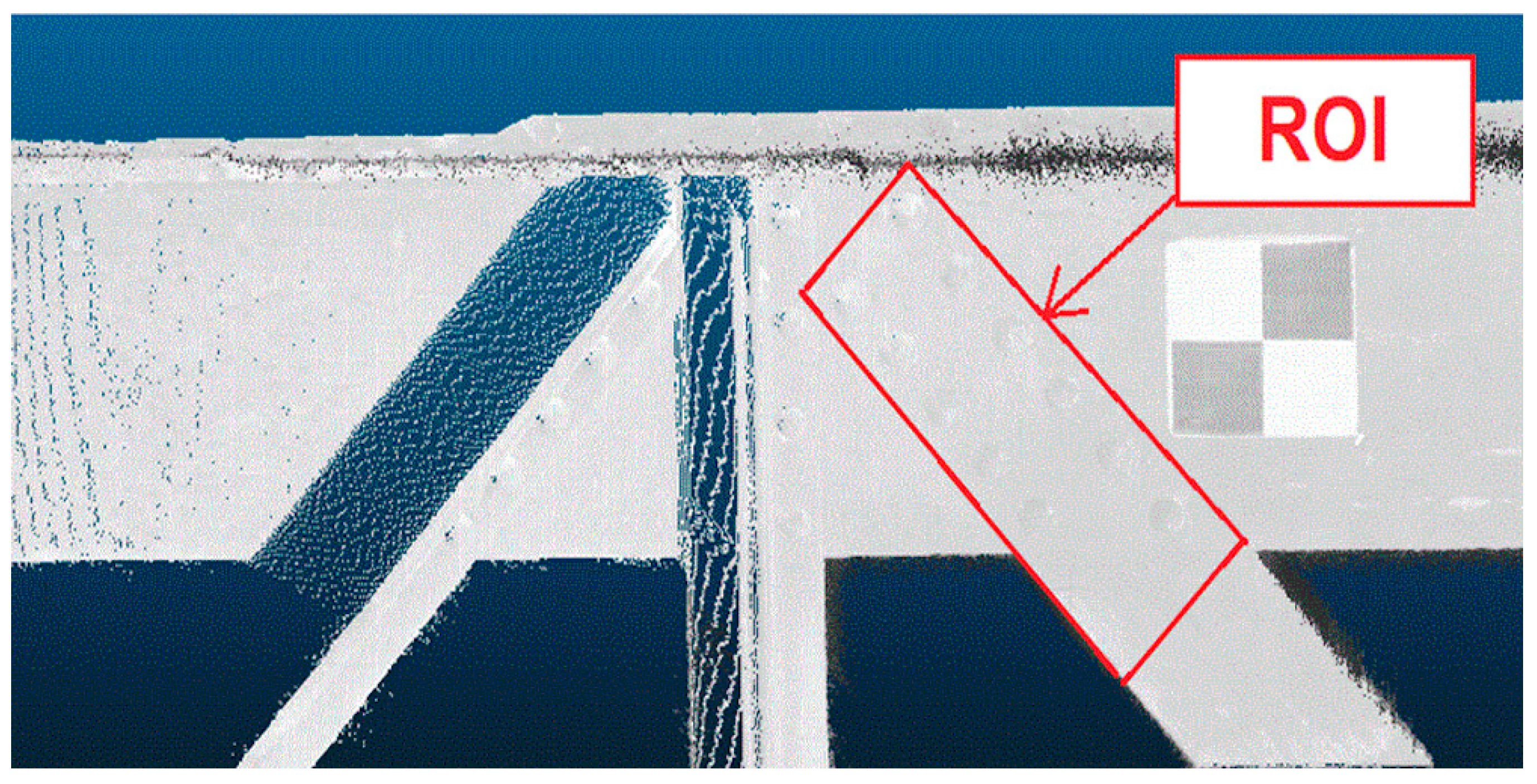
2.1. Identification of the Centers of the Rivets

2.1.1. Determination of the Support Plane of the Rivets

The first step performed by the algorithm is the determination of the support plane of the rivets, plane F-F (Figure 4a). The plane F-F is automatically calculated by hyperplanar fitting of the point cloud using an iterative orthogonal regression procedure [28,29,30]. Initially, the plane is calculated using all points, leaving the plane slightly deviated in the direction of the rivets. Next, the points that are located at a distance greater than 0.5 times the distance from the farthest point are identified (which will coincide with a rivet head). Once these points that will belong to the rivets have been identified, the position of the plane is re-calculated without including them in the regression procedure, thus calculating a second plane that is better adjusted than the first one. This process is carried out two more times, reducing in each step the threshold distance from which points are discarded for the subsequent adjustment of the plane. The threshold distance considered in the last step results from applying a distance equal to two times the laser scanner ranging error $\left(r\right)$. On this basis, the plane that best fits the surface of the ROI is estimated (Figure 4b).

2.1.2. Segmentation of the Rivets

To proceed with the segmentation of the rivets, the points belonging to rivet heads are searched for within the ROI. For this purpose, once the plane F-F has been fitted, the points standing out from the plane are identified. These points constitute the heads of the rivets. The search process is carried out by measuring the orthogonal distance $d{p}_{\left(i\right)}$ between the points $(x_i,y_i,z_i)$ and the plane F-F (see Figure 4c and Equation (1)).

$$d{p}_{\left(i\right)}=abs\left(\frac{A·x_i+B{y}_i+C{z}_i+D}{\sqrt[2]{A^2+B^2+C^2}}\right) i=1,\dots ,n$$

(1)

where $A{x}_i+B{y}_i+C{z}_i+D=0$ is the equation defining the plane F-F and $n$ is the number of points.

If the distance $d{p}_{\left(i\right)}$ exceeds a given threshold value ($nl$) (see Figure 4c), these points are considered as points of the rivet head and thus they are added to the set of points $C\left(x,y,z\right)$ that contains all points belonging to some rivet (Figure 4d).

$$if d{p}_{\left(i\right)}>nl \to \left(x_i,y_i,z_i\right)\in C\left(x,y,z\right)i=1,\dots ,n$$

(2)

where $n$ is the number of points. The threshold value $nl$ is a value that depends on the laser scanner ranging error $\left(r\right)$ specific to each laser scanner model and is calculated according to $nl=r\ast ac$, where $ac$ is an experimentally obtained value. As in the work of Cabaleiro et al. [31], the ac value used in both field and laboratory experiments was 2.

After gathering all points of interest in the set $C\left(x,y,z\right)$, the next step is to group all points that belong to the same rivet head. This grouping is performed by evaluating the distance between the points themselves. The process starts with the point having the greatest vertical distance value $dp\_ma{x}^{\left(1\right)}$. It is worth mentioning here that this type of point is typically located in the central area of the rivet, but in most cases, it does not exactly match the real geometric center of the rivet (see Figure 5a).

Thus, the point with the greatest orthogonal distance $dp\_ma{x}^{\left(1\right)}$ is taken as the search center of the first rivet ($R_1$) (Figure 4a). Next, all points having a distance $d{h}_{\left(i\right)}$ (Figure 5b) less than the diameter of the rivet ($D_k$) are searched for (Equation (3)), and all identified points are assigned to the first rivet ($R_1$) (Equation (4)). The $D_k$ calculation process begins with the smallest normalized rivet diameter ($D_1$) calculating how many points belonging to a rivet head are at distance $D_1$ from the search center point of the rivet $R_1$. The process is then repeated for the second normalized diameter $D_2$. This process is carried out iteratively until the number of points located in a $D_k$ environment of $R_1$ is the same as for a $D_{k+1}$ environment. Thus, the value of $D_k$ for the rivet $R_1$ is obtained.

$$d{h}_{\left(i\right)}=\sqrt{{\left(x_{dp\_max}{}^{\left(1\right)}-x_i\right)}^2+{\left(y_{dp\_max}{}^{\left(1\right)}-y_i\right)}^2+{\left(z_{dp\_max}{}^{\left(1\right)}-z_i\right)}^2}$$

(3)

$$if d{h}_{\left(i\right)}<D_k \to \left(x_i,y_i,z_i\right)\in R_1\left(x,y,z\right)$$

(4)

where $(x_{dp\_max}{}^{\left(1\right)}, y_{dp\_max}{}^{\left(1\right)}, z_{dp\_max}{}^{\left(1\right)})$ are the coordinates of the point with the greatest orthogonal distance $dp\_ma{x}^{\left(1\right)}$ and $\left(x_i,y_i,z_i\right)$ are the coordinates of a point of the point cloud.

In the following, from the group of points still pending of assignment, the point with the second greatest value of the orthogonal distance $dp\_ma{x}^{\left(2\right)}$ is taken as the new center of calculation of the next rivet to be segmented $\left(R_2\right)$, repeating the process described above. This process is applied successively until there is no point left ungrouped. As a result, a full segmentation of each of the rivets is obtained (Figure 5c).

2.1.3. Rivet Center Identification

Once the points belonging to each rivet head have been identified and isolated, their center is calculated. To calculate the center, it must be taken into account that the shape of the rivet head does not follow a regular pattern such as a sphere (see Figure 1c) and that the shape of the rivet head varies from some rivet sizes to others and from some historical structures to others. Additionally, depending on the incident angle of the laser beam, the shape obtained from the point cloud at the base of the rivet is not circular but presenting an important distortion (see Figure 1b). Due to these reasons, a new method for rivet center identification is proposed. This calculation is carried out by means of a weighted average of the spatial position of the points. For it, an importance weight $w_{\left(i\right)}$ is apportioned to each point, where greater weight is assigned to the points farthest from the plane F-F, that is, those with the highest $d{p}_{\left(i\right)}$ values, and therefore closest to the central position. The importance assignment for the points is done taking into account that the points farthest from the plane (F-F) are those that are closest to the position of the center of the rivet (Figure 5a). For a rivet $R_j$, the weight $w_{\left(i\right)}$ of a point $i$ is assigned as a function of the relation between its distance $d{p}_{\left(i\right)}$ from the reference plane (F-F) and the maximum $dp\_{\max }^{\left(j\right)}$ and the minimum $dp\_{\min }^{\left(j\right)}$ distance present in the group of points of the rivet $R_j$ (Equation (5)).

$$w_{\left(i\right)}={\left(\frac{dp\left(i\right)-dp\_mi{n}^{\left(j\right)}}{dp\_ma{x}^{\left(j\right)}-dp\_mi{n}^{\left(j\right)}}\right)}^2 i=1,\dots ,n j=1,\dots ,m$$

(5)

where $n$ is the number of points for each rivet and $j$ is the number of the rivet to be calculated.

In this way, a weighting value $w_{\left(i\right)}$ of one will be assigned to the point with the maximum distance in the group $dp\_{\max }^{\left(j\right)}$ and a value of zero will be assigned to the one that presents the minimum distance $dp\_{\min }^{\left(j\right)}$. After all points on each rivet head have been identified and their importance weight $w_{\left(i\right)}$ assigned, the position of the Theoretical Center of the Rivet ($TCR$) is calculated for each rivet. This process is based on a weighted average of the spatial positions of all points belonging to the same rivet (Equation (6)).

$$\left(x_{TCRj},y_{TCRj},z_{TCRj}\right)=\left(\frac{{{\displaystyle \sum }}_{i=1}^n{x}_i w_i}{{{\displaystyle \sum }}_{i=1}^n{w}_i},\frac{{{\displaystyle \sum }}_{i=1}^n{y}_i w_i}{{{\displaystyle \sum }}_{i=1}^n{w}_i},\frac{{{\displaystyle \sum }}_{i=1}^n{z}_i w_i}{{{\displaystyle \sum }}_{i=1}^n{w}_i}\right) i=1,\dots ,n j=1,\dots ,m$$

(6)

where $\left(x_{TCRj},y_{TCRj},z_{TCRj}\right)$ are the coordinates of the Theoretical Center of the Rivet ($TCR$), n is the number of points for each rivet, and $j$ is the number of the rivet to be calculated. Next, the projection on the support plane of the rivets is carried out, being $Ax+By+Cz+D=0$ the equation of the support plane F-F calculated in Section 2.1.1. and $\left(x_{TCRj},y_{TCRj},z_{TCRj}\right)$ the coordinates of the $TCR$ for the rivet $R_j$. The projected coordinates $\left(x_{TCRpj},y_{TCRpj},z_{TCRpj}\right)$ on the plane F-F are obtained according to the following equations:

$$x_{TCRpj}=x_{TCRj}+\frac{A\ast x_{TCRj}+B\ast y_{TCRj}+C\ast z_{TCRj}+D}{-\left(A^2+B^2+C^2\right)}$$

(7)

$$y_{TCRpj}=y_{TCRj}+\frac{A\ast x_{TCRj}+B\ast y_{TCRj}+C\ast z_{TCRj}+D}{-\left(A^2+B^2+C^2\right)}$$

(8)

$$z_{TCRpj}=z_{TCRj}+\frac{A\ast x_{TCRj}+B\ast y_{TCRj}+C\ast z_{TCRj}+D}{-\left(A^2+B^2+C^2\right)}$$

(9)

$$j=1,\dots ,m$$

where $j$ is the number of the rivet to be calculated. It is very important to note that the relative position between the laser scanner and the riveted joint has a significant effect on the density of the rivet point cloud. This relative position increases the density of points on the face of the rivet located on the side from which it is scanned and decreases the density and distorts the point cloud on the opposite side (Figure 6). Indeed, the point cloud of the rivet on the opposite side of the scanning is more distorted with smaller scanning angles (Figure 1). This effect causes the calculated projected Theoretical Center of the Rivet ($TC{R}_p$) to move towards the laser scanner side as the scanning angle is reduced. In fact, a smaller angle of incidence entails a greater error. To alleviate this issue, an error compensation ($EC$) based on the difference in the density point cloud according to the scanning angle is applied.

First, the area where there is a high density of points in each rivet is calculated. For this purpose, the average density ${\rho }_m$ (points per rivet) of each rivet is taken as a reference. Next, a density point cloud threshold value $U_{\rho }$ is established, where $U_{\rho }=e1\times {\rho }_m$, being $e1$ a constant value obtained experimentally ($e1$ = 1/50 from laboratory testing and field experiments). The neighborhood of each point (in a radius of D_k/10) is analyzed and if the density of points in such a neighborhood exceeds $U_{\rho }$, then that point will be identified as belonging to a high-density area. Once the high-density points have been identified, its geometric center is calculated by using a simple average (Equation (10)). This point will be named as the Center of Concentration points of the Rivet ($CCR$). Subsequently, the projection of the $CCR$ on the support plane will be carried out, obtaining the $CC{R}_p$.

$$\left(x_{CCRj},y_{CCRj},z_{CCRj}\right)=\left(\frac{{{\displaystyle \sum }}_{k=1}^q{x}_k }{\mathrm{q}},\frac{{{\displaystyle \sum }}_{k=1}^q{y}_k }{\mathrm{q}},\frac{{{\displaystyle \sum }}_{k=1}^q{z}_k }{\mathrm{q}}\right) k=1,\dots ,q j=1,\dots ,m$$

(10)

where $\left(x_{CCRj},y_{CCRj},z_{CCRj}\right)$ are the coordinates of the Center of Concentration points of the Rivet ($CC{R}_j$), q is the number of points belonging to a high-density area, and $m$ is the number of the rivet to be calculated.

The Theoretical Center of the Rivet ($TCR$) (as already mentioned at the beginning of the methodology) will deviate from the Real Center of the Rivet ($RCR$) as the scanning angle is reduced. The same occurs with the Center of Concentration points of the Rivet $CCR$ (although more intensely) due to the fact that only the points present in the high-density area are used for its calculation. For scanning positions close to 90°, it has been experimentally verified that the position of the projected $RC{R}_p$ coincides with the position of the projected $TC{R}_p$ and the position of the projected $CC{R}_p$. The vector joining the projected $TC{R}_p$ and the projected $CC{R}_p$ indicates the scanning direction (Figure 6), and the distance between these two points ($L_i$) is given by Equation (11).

$$L_j=\sqrt{{\left(x_{CCRpj-}{x}_{TCRpj}\right)}^2+{\left(y_{CCRpj-}{y}_{TCRpj}\right)}^2+{\left(z_{CCRpj-}{z}_{TCRpj}\right)}^2 }j=1,\dots ,m$$

(11)

where $\left(x_{CCRpj},y_{CCRpj},z_{CCRpj}\right)$ are the coordinates of the projected Center of Concentration points of the Rivet ($CC{R}_p$), $\left(x_{TCRpj},y_{TCRpj},z_{TCRpj}\right)$ are the coordinates of the projected Theoretical Center of the Rivet ($TC{R}_p$), and $j$ is the number of the rivet to be calculated.

To find the coordinates of the projected Real Center of the Rivet $RC{R}_p$, an error compensation $EC$ equal to $L_j$ is applied to the projected Theoretical Center of the Rivet ($TC{R}_p$) in the direction joining the $TC{R}_p$ with the $CC{R}_p$ (Figure 7). The $L_j$ value is a heuristic value deemed as adequate for using as error compensation $EC$, which has been deduced and verified from experimental testing.

Once the projected Real Center of the Rivet ($RC{R}_p$) has been calculated, the distances of the 10 points of the high-density area furthest from the projected Real Center of the Rivet ($RC{R}_p$) are calculated. The arithmetic mean of these distances is then calculated and the closest normalized rivet radius above this value is the radius of the rivet used.

2.1.4. Data File Generation

Once the coordinates of the Real Center of each Rivet $RC{R}_p$ have been calculated, a file with these data is generated to be posteriorly exported to the 3D HBIM model. Once this has been done, all the data are simply stored in a standard data file, such as a *.txt file. It is worth noting that all coordinates are already expressed in the global reference system of the structure.

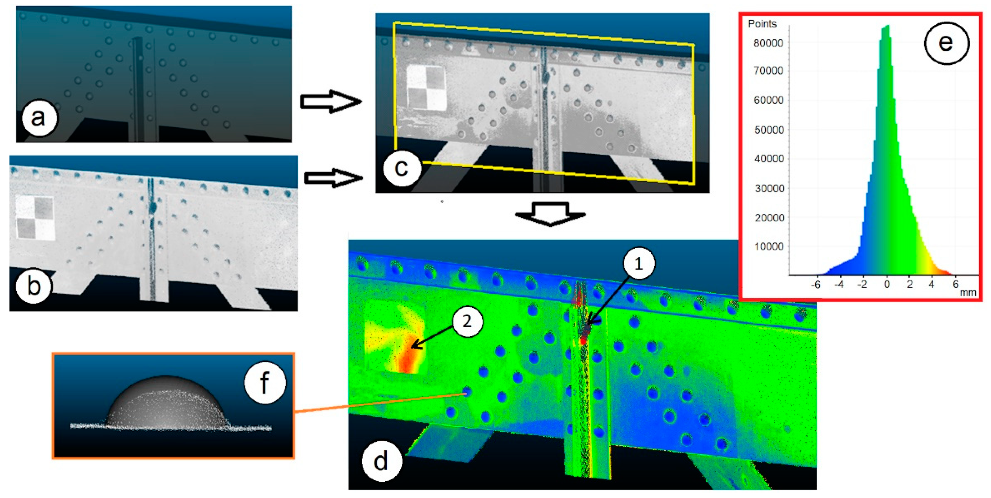
2.2. Three-Dimensional Modeling of the Rivets

Once the 3D model of the structure has been created (assuming that the global reference system is the same as that of the point cloud), the 3D modeling process of the rivets is carried out according to the following steps:

-

Import the data files containing the Cartesian coordinates of the centers of the rivets.

-

Projection of these points on the surface of the corresponding structural profiles.

-

Generation of the 3D model of the rivets in each of the projection points. Generally, the modeling of the rivet head is carried out as a hemisphere using the diameter of the rivet, although in reality the rivet is not perfectly hemispherical, but this simplification is accurate enough and takes up little memory space in the final geometrical model. By modeling each rivet in its actual position, a more detailed HBIM model can be obtained, which can be very useful for the structural safety assessment and health monitoring over time.

3. Laboratory Testing

3.1. Materials

Matlab was used to develop the algorithm, CloudCompare for the processing of the point cloud, and SolidWorks for the geometrical modeling. A Faro Focus 3D laser scanner (FARO Technologies, Inc., Florida, U.S.) was used for the data acquisition phase, which allows distances to be measured in a range of 1.0 to 120.0 m with a ranging error of ±2.0 mm. To evaluate the efficiency and precision of the proposed methodology, the algorithm will be applied to the point cloud of several rivets whose dimensions and positions are precisely known. This test aims to check the deviation between the results obtained with the algorithm with respect to the tested specimens. For these tests, three 3D models were designed that simulated the shape of a riveted surface with different sizes of rivets for each specimen. The specimens were subsequently manufactured using an Ultimaker 2+ 3D printer with a minimum precision of 0.13 mm. Subsequently, the specimens were scanned in the laboratory using the FARO Focus laser scanner. Different scanning angles and densities were employed to evaluate the precision of the algorithm. These models contained hemispheres that simulated the shape of a theoretical hemispherical rivet, with their normalized dimensions according to the standards [32].

The specimens used were a plate of 215 × 50 mm with four 25-mm diameter rivets, a plate of 215 × 70 mm with three 32-mm diameter rivets, and a plate of 215 × 70 mm with three 40-mm diameter rivets. The scanner was placed at the same height as the specimens and five scans at different angles (see Figure 8) with respect to the rivets were performed. These scans were done with a high density (mean of 0.8 mm between points). After the first series was completed, the scanning density was reduced to an average of 2.0 mm between points on the surface of the rivets. With low density, the scans were performed again at all five positions. Both the positions and the density used represent different positions and densities which are typical on the in situ scanning of real structures. The ROI containing the rivets was taken to search for the rivets with the algorithm. The coordinates of a corner in each model were taken as a reference in order to verify the results in the calculation of the position of the center of the rivets.

3.2. Results

The bar graphs in Figure 9 show the mean error (mm) obtained in calculating the center position of the rivets according to the scanning angle, rivet diameter, and the scanning density when applying the algorithm to the laboratory specimens. The error is defined as the Euclidean distance between the real position of the center of the rivets and the one derived from the application of the proposed algorithm. This error is not systematic and although it is usually in the scanning direction, it may also take place in other different directions with respect to the rivet center. Figure 8a shows that for low-density scanning and for the worst-case scenario (scanning angle of 15° and rivet diameter of 40 mm) the mean error without compensation (EC) was 7.1 mm. After applying (EC), the mean error was reduced to 3.0 mm. Similarly, Figure 8b shows that for the worst-case scenario (scanning angle of 15° and rivet diameter of 40 mm) but for high-scanning density, the mean error without compensation (EC) was 3.5 mm. After applying (EC), the mean error was reduced to 1.6 mm. Considering all variables (scanning angle, rivet diameter, and the scanning density) and applying the compensation ($EC$), the average global error committed when calculating the center position is 1.4 mm; a 53% reduction. Moreover, the maximum error for any single case is 3.5 mm (see also Figure 10).

The bar graphs in Figure 11 shows the normalized error with respect to the rivet diameter according to the scanning angle and the scanning density. The improvement in the mean of the global error that is achieved with the compensation ($EC$) was the same as in the previous case (53%).

Moreover, Figure 10 shows a box plot of the errors (with the compensation $EC$ already applied) for both low- and high-density point clouds as a function of the rivet diameter. As can be seen, in all cases the median of the error increases with the rivet diameters. The highest error values are committed with the largest diameter. In any case, the maximum single error does not exceed 3.5 mm.

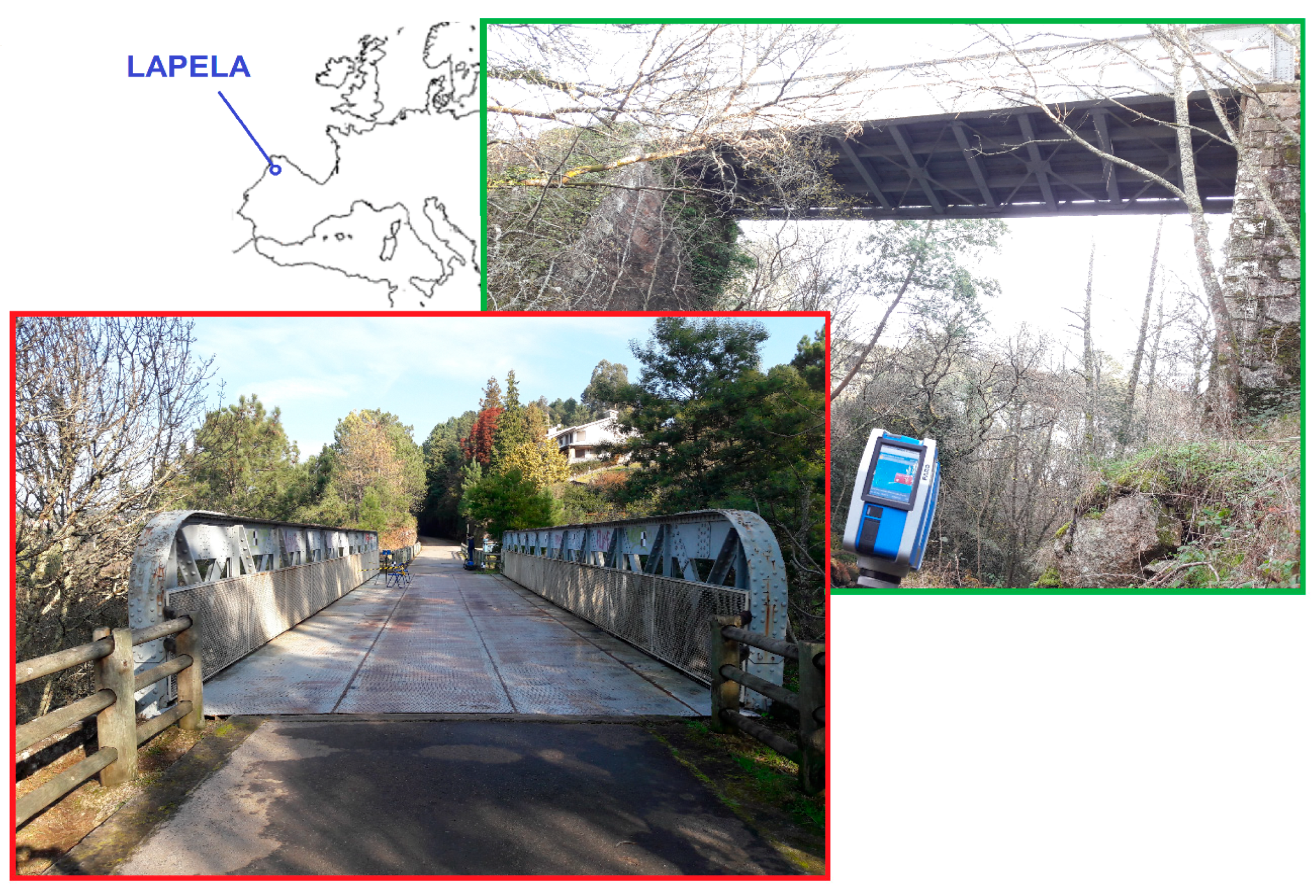
4. Real Case Study

4.1. Description of the Bridge

The developed algorithm was also tested on a full-scale real bridge. The case study considered was the historic steel bridge of Lapela (Figure 12).

This bridge belongs to the old railway line between Valença and Monçao (Portugal). It was built in 1915 and closed down in 1989. In 2004, the old railway line was converted into an eco-track. The bridge and the medieval tower of Lapela are two emblematic architectural elements of this eco-track and this area near the Miño River, on the border with Spain. The bridge is 20.0 m long and 5.0 m wide. Due to its architectural value, a 3D as-built model was elaborated in as much detail as possible and the assessment of structural safety and health monitoring over time will be a necessary task. The bridge is built from L-shaped steel profiles and plates joined by rivets. The vast majority of rivets have a diameter of 40 mm. The structure was scanned, and as indicated above, the 3D modeling process was carried out using the same global reference system as that employed for the point cloud registration. The files containing the coordinates of the rivets extracted by means of the developed algorithm were imported into this 3D model (Figure 13). As it was also previously described, these coordinates were projected onto the surface of the corresponding structural profiles so that the 3D modeling of the rivets was finally performed on the basis of each of these projection points. In this way, a quite detailed 3D HBIM model can be finally achieved.

Lastly, the deviation of the generated 3D model of the rivets from their real positions in the steel joints was verified. For this purpose, the 3D solid model of the bridge was compared with the scanned point cloud using the inbuilt capabilities of CloudCompare software. The results obtained in the 3D modeling were not compared with measurements made directly on the rivets of the bridge because, due to the difficult in situ conditions, manual measurements could have even more error than those obtained directly from the point cloud, which has a maximum error of ±2.0 mm. This comparison is done with each of the scans in global coordinates; that is, the overall registered point cloud is not used, but each of the single scans is used. In this way, it is possible to avoid including the registration error, which is about 2.0 mm, in the process [33].

4.2. Results and Discussion

Figure 14 shows, as an example, the comparison between the model with rivets of one of the steel joints of the bridge and the corresponding point cloud. Once the point cloud is overlapped on the 3D model of the riveted joint, the distances between them are calculated by means of the “Compute cloud/mesh distance” function of CloudCompare, obtaining the results shown in Figure 14d and quantified in the histogram in Figure 14e. This histogram shows the deviation for each zone of the point cloud in the form of a color code (clusters). The rivet heads (displayed in blue) show a negative deviation; that is, the model protrudes above the point cloud. This effect is because the rivets have been modeled as regular hemispheres (mainly for the sake of simplifying the modeling process) while the real ones have a flatter head due to the riveting process (see Figure 14f).

The only rivets whose position was poorly identified are those marked as “1” in Figure 14d. This is due to the fact that the point cloud used is a frontal one. In this frontal point cloud, the rivets perpendicular to the plane (i.e., located on the steel plate) or even within a range of 90 to 30° are perfectly defined. However, those rivets joining the vertical L-shaped profiles were taken from a scanning angle of less than 10°, making them impossible to identify; this also happens in a similar way in the diagonal of Figure 15a. For the correct identification of these rivets, it would be necessary to resort to a point cloud scanned from a more open position (with a scanning angle of 30° or more).

Figure 15 shows a comparison between the 3D model and the point cloud of other bridge riveted joints. Figure 15b details the union of one of the sides of the bridge, where it was decided to leave a rivet in the upper right part without modeling in order to check whether its incorrect modeling would be properly detected. As can be seen, this error was clearly detected.

Table 1. Statistical estimators (mean and standard deviation) describing the discrepancies between the 3D modeling and the point clouds of the rivets in Figure 16.

Rivet (N°)	Mean (mm)	Std.dev (mm)	Rivet (N°)	Mean (mm)	Std.dev (mm)	Rivet (N°)	Mean (mm)	Std.dev (mm)	Rivet (N°)	Mean (mm)	Std.dev (mm)
1	0.07	0.57	12	−0.09	0.42	23	−1.45	1.48	34	−1.32	1.42
2	0.40	0.60	13	−0.25	0.52	24	−1.73	0.96	35	−1.40	0.73
3	−0.30	0.57	14	−0.34	0.55	25	−0.78	1.12	36	−1.80	0.53
4	−0.86	0.45	15	0.36	0.58	26	−1.31	1.61	37	−0.75	0.53
5	0.16	0.57	16	−1.31	0.85	27	−0.50	1.24	38	−1.12	0.62
6	−0.67	0.78	17	−1.65	1.16	28	0.89	1.12	39	−0.97	0.59
7	−0.57	0.45	18	−1.03	0.87	29	−0.73	1.13	40	−1.55	0.89
8	−1.43	0.52	19	−1.18	1.35	30	−0.73	1.14	41	−1.48	0.74
9	−1.05	0.52	20	−1.78	1.13	31	−0.59	1.56	42	−1.67	0.83
10	−0.22	0.50	21	−1.59	0.87	32	0.26	1.33	43	1.99	1.19
11	−0.05	0.71	22	−1.91	0.89	33	−1.32	1.43	44	−1.95	1.03

shows the discrepancies between the 3D modeling of the rivets of Figure 16 with their real shape (point clouds).

As indicated in the previous section, the results of the laboratory tests with specimens were satisfactory, even for scanning angles of 15°. However, in the in situ scanning of the Lapela bridge, numerous defects on the point clouds of the rivets were observed for scanning angles less than 30°. Hence, based on these results, it is recommended to work with scanning angles between 90° and 30°. In general, for the Lapela Bridge, the deviation in the correct positioning of the rivets is on average 2.0 mm. These results confirm the data obtained in the laboratory, which summarize the error committed by the algorithm in the identification of the center of the rivets around 5.0% of the diameter. Through the whole comparison process, significant errors were only found in the rivets that present an angle of less than 15° with respect to the position of the scanner.

Finally, it is worth mentioning that if one bears in mind the structural assessment stage, taking into account the exact number of rivets and their correct positioning might substantially affect the results of assessment of the local condition of the joint. Accordingly, Figure 17a details an analysis with the explicit modeling of the rivets, where areas of high-stress concentration can be detected (especially in the holes of the continuous plate of the bridge, Figure 17a, top), while when rivets are not considered and a continuous joint is modeled (Figure 17b), no significant stress concentration appears. These areas of high stress must be taken into account in the structural analysis because if they are excessively large or close to a beam edge, they can be dangerous. Figure 18 shows the difference in the results between when the rivets are correctly located (Figure 18a) and when the rivets have a location error of 7.0 mm (Figure 18b). According to the results of Figure 18b, the yield strength is exceeded in the entire outer area of the steel profile. Therefore, the profile would yield locally, leading to a possible shear-out failure, a result that would not be real because the rivet has been incorrectly modeled. Thus, the explicit inclusion of the rivets in the numerical models in their correct location is a desirable feature for the local detailed structural analysis of the joint.

5. Conclusions

Many riveted steel structures are considered a fundamental part of our historical heritage and a large number of them are still in service. Due to this, the maintenance, control, and conservation of these structures is a priority task. HBIM technology and Lidar data are presented as fundamental tools for this aim. For HBIM, it is necessary to build 3D models that accurately reflect the current and actual condition of these constructions. In this sense, rivets are a fundamental element to be modeled, but currently, this modeling process is manual and tedious.

The main contribution of this work is the development of a methodology and its corresponding algorithms that allow the automatic identification of the rivets, the extraction of the coordinates of their center and diameter, and the subsequent automatic 3D geometrical modeling from laser scanning data of the structure. In this way, a more detailed HBIM model can be obtained, which can very useful for the structural safety assessment and health monitoring over time.

The precision reached in laboratory conditions in the automatic identification of the rivet center is adequate, with an average global error value of 1.4 mm and a maximum single error of 3.5 mm. Although in laboratory testing it was verified that the results were correct up to scanning angles of 15°, in the application of the developed algorithm to a full-scale real case study, it was verified that to obtain adequate results the scanning angle with respect to the rivets should be between 90° and 30°. Although this work has focused on the rivets, future works could also address the searching of bolts, since this is another form of joining system commonly used in more recent steel structures.

References

- López, F.J.; Lerones, P.M.; Llamas, J.; Gómez-García-Bermejo, J.; Zalama, E. A review of heritage building information modelling (H-BIM). Multimodal Technol. Interact. 2018, 2, 21. [Google Scholar] [CrossRef]
- Pierdicca, R.; Paolanti, M.; Matrone, F.; Martini, M.; Morbidoni, C.; Malinverni, E.S.; Frontoni, E.; Lingua, A.M. Point Cloud Semantic Segmentation Using a Deep Learning Framework for Cultural Heritage. Remote Sens. 2020, 12, 1005. [Google Scholar] [CrossRef]
- Mol, A.; Cabaleiro, M.; Sousa, H.S.; Branco, J.M. HBIM for storing life-cycle data regarding decay and damage in existing timber structures. Autom. Constr. 2020, 117, 103262. [Google Scholar] [CrossRef]
- Andriasyan, M.; Moyano, J.; Nieto-Julián, J.E.; Antón, D. From Point Cloud Data to Building Information Modelling: An Automatic Parametric Workflow for Heritage. Remote Sens. 2020, 12, 1094. [Google Scholar] [CrossRef]
- Palomar, I.J.; Valldecabres, J.L.G.; Tzortzopoulos, P.; Pellicer, E. An online platform to unify and synchronise heritage architecture information. Autom. Constr. 2020, 110, 103008. [Google Scholar] [CrossRef]
- Croce, V.; Caroti, G.; De Luca, L.; Jacquot, K.; Piemonte, A.; Véron, P. From the Semantic Point Cloud to Heritage-Building Information Modeling: A Semiautomatic Approach Exploiting Machine Learning. Remote Sens. 2021, 13, 461. [Google Scholar] [CrossRef]
- Maalek, R.; Lichti, D.D.; Ruwanpura, J.Y. Automatic recognition of common structural elements from point clouds for automated progress monitoring and dimensional quality control in reinforced concrete construction. Remote Sens. 2019, 11, 1102. [Google Scholar] [CrossRef]
- Cui, Y.; Li, Q.; Dong, Z. Structural 3D Reconstruction of Indoor Space for 5G Signal Simulation with Mobile Laser Scanning Point Clouds. Remote Sens. 2019, 11, 2262. [Google Scholar] [CrossRef]
- Karunathilake, A.; Honma, R.; Niina, Y. Self-Organized Model Fitting Method for Railway Structures Monitoring Using LiDAR Point Cloud. Remote Sens. 2020, 12, 3702. [Google Scholar] [CrossRef]
- Cabaleiro, M.; Riveiro, B.; Arias, P.; Caamano, J.C. Algorithm for beam deformation modeling from LiDAR data. Measurement 2015, 76, 20–31. [Google Scholar] [CrossRef]
- Herraez, J.; Navarro, P.; Denia, J.L.; Martin, M.T.; Rodriguez, J. Modeling the thickness of vaults in the church of Santa Maria de Magdalena (Valencia, Spain) with laser scanning techniques. J. Cult. Herit. 2014, 15, 679–686. [Google Scholar] [CrossRef]
- Cabaleiro, M.; Riveiro, B.; Arias, P.; Caamano, J.C.; Vilan, J.A. Automatic 3D modelling of metal frame connections from LIDAR data for structural engineering purposes. ISPRS J. Photogramm. Remote Sens. 2014, 96, 47–56. [Google Scholar] [CrossRef]
- Yin, X.; Liu, H.; Chen, Y.; Al-Hussein, M. Building information modelling for off-site construction: Review and future directions. Autom. Constr. 2019, 101, 72–91. [Google Scholar] [CrossRef]
- Santos, R.; Costa, A.A.; Silvestre, J.D.; Pyl, L. Informetric analysis and review of literature on the role of BIM in sustainable construction. Autom. Constr. 2019, 103, 221–234. [Google Scholar] [CrossRef]
- Garzia, F.; Costantino, D.; Baiocchi, V. Security and safety management and role of laser scanning in unique and peculiar cultural heritage sites such as the papal basilica and the sacred convent of Saint Francis in Assisi in Italy. Int. J. Herit. Archit. 2018, 2, 271–282. [Google Scholar] [CrossRef]
- Cuartero, J.; Cabaleiro, M.; Sousa, H.S.; Branco, J.M. Tridimensional parametric model for prediction of structural safety of existing timber roofs using laser scanner and drilling resistance tests. Eng. Struct. 2019, 185, 58–67. [Google Scholar] [CrossRef]
- Sanchez-Aparicio, L.J.; Riveiro, B.; Gonzalez-Aguilera, D.; Ramos, L.F. The combination of geomatic approaches and operational modal analysis to improve calibration of finite element models: A case of study in Saint Torcato church (Guimaraes, Portugal). Constr. Build. Mater. 2014, 70, 118–129. [Google Scholar] [CrossRef]
- Yang, L.; Cheng, J.C.; Wang, Q. Semi-automated generation of parametric BIM for steel structures based on terrestrial laser scanning data. Autom. Constr. 2020, 112, 103037. [Google Scholar] [CrossRef]
- Basta, A.; Serror, M.H.; Marzouk, M. A BIM-based framework for quantitative assessment of steel structure deconstructability. Autom. Constr. 2020, 111, 103064. [Google Scholar] [CrossRef]
- Laefer, D.F.; Truong-Hong, L. Toward automatic generation of 3D steel structures for building information modelling. Autom. Constr. 2017, 74, 66–77. [Google Scholar] [CrossRef]
- Donato, V.; Biagini, C.; Bertini, G.; Marsugli, F. Challenges and opportunities for the implementation of h-bim with regards to historical infrastructures: A case study of the ponte giorgini in castiglione della pescaia (grosseto-italy). Int. Arch. Photogramm. Remote Sens. Spat. Inf. Sci. 2017, 42. [Google Scholar] [CrossRef]
- Morganti, R.; Tosone, A.; Di Donato, D.; Abita, M. Hbim and the 20th century steel building heritage–a procedure suitable for the construction history in italy. Int. Arch. Photogramm. Remote Sens. Spat. Inf. Sci. 2019. [Google Scholar] [CrossRef]
- Xie, Q.; Lu, D.; Du, K.; Xu, J.; Dai, J.; Chen, H.; Wang, J. Aircraft Skin Rivet Detection Based on 3D Point Cloud via Multiple Structures Fitting. Comput. Aided Des. 2020, 120, 102805. [Google Scholar] [CrossRef]
- Ying, C.; Zhou, Y.; Han, D.; Qin, G.; Hu, K.; Guo, J.; Guo, T. Applying BIM and 3D laser scanning technology on virtual pre-assembly for complex steel structure in construction. In Proceedings of the IOP Conference Series: Earth and Environmental Science, Beijing, China, 20–22 September 2019; Volume 371, p. 022036. [Google Scholar] [CrossRef]
- Nurunnabi, A.; Sadahiro, Y.; Laefer, D.F. Robust statistical approaches for circle fitting in laser scanning three-dimensional point cloud data. Pattern Recognit. 2018, 81, 417–431. [Google Scholar] [CrossRef]
- Truong-Hong, L.; Laefer, D.F. A semi-automatic member detection for metal bridges. In Proceedings of the IABSE Conference Nara: Elegance in Structures, Nara, Japan, 13–15 May 2015; Available online: http://hdl.handle.net/10197/7447 (accessed on 24 May 2021).
- Kim, M.K.; Sohn, H.; Chang, C.C. Automated dimensional quality assessment of precast concrete panels using terrestrial laser scanning. Autom. Constr. 2014, 45, 163–177. [Google Scholar] [CrossRef]
- Leng, L.; Zhang, T.; Kleinman, L.; Zhu, W. Ordinary least square regression, orthogonal regression, geometric mean regression and their applications in aerosol science. J. Phys. Conf. Ser. 2007, 78, 012084. [Google Scholar] [CrossRef]
- Shapiro, L.S.; Brady, M. Rejecting outliers and estimating errors in an orthogonal-regression framework. Philos. Trans. R. Soc. Lond. Ser. A Phys. Eng. Sci. 1995, 350, 407–439. [Google Scholar] [CrossRef]
- Maronna, R. Principal components and orthogonal regression based on robust scales. Technometrics 2005, 47, 264–273. [Google Scholar] [CrossRef]
- Cabaleiro, M.; Lindenbergh, R.; Gard, W.F.; Arias, P.; van de Kuilen, J.W.G. Algorithm for automatic detection and analysis of cracks in timber beams from LiDAR data. Constr. Build. Mater. 2017, 130, 41–53. [Google Scholar] [CrossRef]
- España. Ministerio de Obras Públicas y Transportes. Norma básica de la edificación NBE MV-105 1967: Roblones de acero Normativas. España. Ministerio de Obras Públicas y Transportes: 1992. ISBN 8474338042, 9788474338041. Available online: https://www.boe.es/eli/es/rd/1995/11/10/1829 (accessed on 21 March 2021).
- Riveiro, B.; Morer, P.; Arias, P.; De Arteaga, I. Terrestrial laser scanning and limit analysis of masonry arch bridges. Constr. Build. Mater. 2011, 25, 1726–1735. [Google Scholar] [CrossRef]