Article

Estimation of Rangeland Production in the Arid Oriental Region (Morocco) Combining Remote Sensing Vegetation and Rainfall Indices: Challenges and Lessons Learned

1
Department of Environmental Sciences and Management, University of Liege, 185 Avenue de Longwy, 6700 Arlon, Belgium
2
Centre Régional de la Recherche Agronomique d’Oujda, Institut National de la Recherche Agronomique Maroc, Oujda 60000, Morocco
*
Author to whom correspondence should be addressed.
Remote Sens. 2021, 13(11), 2093; https://doi.org/10.3390/rs13112093
Submission received: 27 April 2021 / Revised: 20 May 2021 / Accepted: 24 May 2021 / Published: 26 May 2021
(This article belongs to the Special Issue Deep Learning Methods for Crop Monitoring and Crop Yield Prediction)

Abstract

:
This study aimed at investigating the potential of vegetation indices and precipitation-related variables derived from remote sensing to assess rangeland production in the arid environment of the Moroccan Oriental region and identifying the challenges linked to that particular biome. Vegetation indices (VIs) and the Standardized Precipitation Index (SPI) computed at various aggregation periods were first integrated into a Random Forest model. In a second step, we studied in more detail the linear relationship between rangeland biomass and one of the spectral indices (ARVI) for the various vegetation formations present in the area. We concluded that, mostly due to the presence of alfa steppes (Stipa tenacissima), and especially to a large proportion of non-photosynthetic vegetation, it is not possible to accurately estimate rangeland production with a global model in this region. We recommend separating Stipa tenacissima from the other species in models and focusing on methods aimed at studying dry and non-photosynthetic vegetation to improve the quality of the prediction for alfa steppes.

Graphical Abstract

1. Introduction

Arid and semi-arid regions are part of dryland ecosystems, which are characterized by low and variable precipitation in both time and space [1,2,3], combined with high evapotranspiration. They cover about 25% (arid: 10%, semi-arid: 15%) of the surface of the planet and are home to one billion people [4,5].
Rangeland makes up 87% and 54% of the land use in arid and semi-arid areas [4]. In these regions, the preservation of the integrity of rangeland presents both economic and environmental interests. Indeed, drylands and their vegetation cover provide a series of ecosystem services, including an important source of food and income for the local population through livestock keeping, and involvement in a series of environment-related processes such as the regulation of climate through carbon sequestration and soil–atmosphere energy exchanges, contribution to soil nutrient cycles, regulation of the hydrological cycle, protection against soil erosion, etc. [1,4,6,7].
In these regions, rangeland properties, including biomass production, are driven in a large part by climatic conditions and more specifically the availability of water [1,3,4,8,9,10]. In the current context of climate change, rangeland areas are subject to an increase in climate hazards, especially in the variability of rains [9,11], and local increases in drought episodes (e.g., in the Mediterranean region: [11]), causing important variations in forage yield from year to year [10,12]. The degradation of the vegetation cover caused by natural conditions is aggravated in these areas by increased pressure due to population growth and the demand for more food, economic development, technological progress, etc., causing alterations in the vegetation cover, including losses in biomass, by human-induced factors such as overgrazing or transformation of rangeland into cultivated areas [2,4,13,14,15,16].
This context highlights the need for the proper assessment of the vegetation cover, both in terms of quantity (biomass, fraction of soil covered by vegetation, etc.) and quality (disappearance of the original species in favor of species indicating land degradation, etc.) that can be incorporated in a plan for the sustainable management of rangeland that integrates both the protection of livelihoods of local populations and the preservation of this already fragile environment. The assessment of rangeland biomass over large areas, such as at regional or national level, therefore constitutes an important economic and environmental tool that allows for the better management of grazing areas.
In arid and semi-arid regions, characterized by vast areas that are sometimes difficult to reach, the integration of remote sensing data has become over the past few decades a widely used method to study and describe the vegetation cover and its variations in space and time [6,17]. Combinations of the R and NIR bands, in the form of a simple ratio or other linear combinations such as the Normalized Difference Vegetation Index (NDVI) [18], the Enhanced Vegetation Index [19], and several variations of the Soil-Adjusted Vegetation Index [20,21,22,23], have been extensively used to monitor changes in vegetation all over the globe and assess a variety of biophysical properties, including plant biomass (a list of studies is available in reviews by [24], for rangelands and grasslands by [17,25], and in arid and semi-arid regions by [6].
A family of Soil-Adjusted Vegetation Indices was designed to attenuate the effects of variations in the brightness of the soil background on the observed reflectance spectra and on derived vegetation indices (VIs). In [20] the Soil-Adjusted Vegetation Index (SAVI) was created by adapting the NDVI by addition of an adjustment factor (L), dependent on the fraction of green vegetation (L varying from 0.25 for high vegetation densities to 1 for sparsely vegetated areas). A series of adaptations have been made to the original Soil-Adjusted Vegetation Index starting with the Transformed Soil-Adjusted Vegetation Index (TSAVI) which was introduced to generalize the SAVI to situations where the soil line parameters differ from the default one (slope = 1 and intercept =0) [21,26]. In [22], the L factor in SAVI was adapted and a self-adjusting factor was introduced in the Modified Soil-Adjusted Vegetation Index (MSAVI) that is able to minimize the influence of soil background without prior knowledge of the fraction of canopy cover. Finally, the SAVI equation was simplified (Optimized Soil-Adjusted Vegetation Index, OSAVI) [23] by introducing a constant χ parameter that allows for a reduction in the soil background effects in the absence of information on soil properties. The Enhanced Vegetation Index (EVI) [19] was similarly introduced to reduce the influence of variations in the canopy background and, in addition, to correct for effects of atmospheric aerosol.
In arid regions, the above-mentioned indices have been used to assess biomass in rangelands covered by a variety of species including perennial grasses, shrubs, and annual herbaceous vegetation in Africa [27,28,29,30,31,32], North America [33], South America [34], Australia [35], the Middle East [36,37,38] and Mongolia [39,40,41].
Additionally, the Atmospherically Resistant Vegetation Index (ARVI) [42,43], designed to mitigate the influence of aerosol thanks to the addition of information from the blue channel, and the Structure Insensitive Pigment Index (SIPI) [44], which allows one to derive photosynthetic pigments information (more specifically, the ratio between chlorophyll-a and carotenoids) for vegetation formations characterized by variable canopy structures by reducing the influence of the leaf surface and internal structure, can be of particular interest in arid and semi-arid regions. Although they are less commonly found in the literature concerning the estimation of biomass in arid and semi-arid regions, these indices are worth being investigated in such environments due to their particular properties. Indeed, since arid and semi-arid regions constitute a major source of dust aerosol [45,46], built-in atmospheric correction is a desirable feature for vegetation indices used in the area. Besides, an index that is less sensitive to variations in canopy structure could prove useful in an environment characterized by a heterogeneous vegetation cover, as it is the case of our region of interest where various species of shrubs are found along with annual and perennial herbaceous vegetation depending on the level of degradation of the area [16].
Reflectances in the shortwave infrared (SWIR) region (0.86 and 1.24 µm) were combined to build the Normalized Difference Water Index (NDWI) [47], allowing one to assess the liquid water content of vegetation and to discriminate between green (positive values of NDWI) and dry vegetation (negative values of NDWI). Indices designed to be sensitive to the water contents, including NDWI, have been used in arid and semi-arid regions to monitor the production of vegetation, for example, in [32,33,34,40].
In arid and semi-arid regions, where vegetation growth is conditioned by water availability, drought indices, including the Standardized Precipitation Index (SPI), are used frequently in combination with vegetation indices [37,48,49,50,51,52] but also with in situ biomass measurements [53] to assess the effects of drought on the vegetation cover for a variety of land uses and land covers, including rangeland, cultivated areas, etc. In addition, in arid and semi-arid regions, the association of precipitation-related to remote sensing biophysical variables was shown to improve the prediction of biomass [54]. The Standardized Precipitation Index was introduced as a way to describe precipitation patterns in terms of probabilities for a set of time scales relevant to the various usable water sources [55]. It compares precipitation for a specific accumulation period to the long-term distribution and allows for a uniform characterization of rainfall for the different time scales [55,56]. Negative values are synonyms of below-average rainfall conditions, with increasing severity of drought as SPI decreases [55], while positive values mean above average water input for the period of interest. The various lengths of the accumulation period reflect the duration of the phenomena involved in the water cycle with their specific effects (with, for example, short-term accumulation periods (1–3 months) linked to immediate impacts such as reduced soil moisture) [56,57,58]. In terms of impacts of precipitation on vegetation, accumulation periods from 1 to 6 months are suggested to monitor agricultural drought [58] as it provides a seasonal estimation of precipitation but longer time scales (inter-seasonal) are also mentioned [58] as drought can progress over time and continue to impact vegetation. While reference [48] mentions short to medium periods of influence (4 to 6 months) for precipitation events on the evolution of vegetation in arid and semi-arid regions, other studies [49,50,51,52,53,54,55,56,57,58,59,60] found that vegetation properties are impacted by precipitation periods cumulated over longer time series (12 months and more).
As larger volumes of Earth observation data become available, thanks to increased spatial and spectral resolutions, an increased number of active satellites, longer time series, etc., more information is produced, creating a need for fast and robust processing methods [61] while providing an opportunity to describe more complex phenomena linked to the characterization of the Earth’s surface, including its vegetation cover. In this context, machine learning algorithms are of particular interest, as they allow for the integration of a great number of variables, including a combination of variables of different types (continuous and categorical), into models aimed at assessing the vegetation’s properties [61]. In addition, these algorithms require no prior knowledge on data distribution and therefore allow the description of complex and non-linear interactions [61,62,63].
Parametric approaches, such as linear and multilinear regression, have long been the preferred method in remote sensing applications [61,62], including for the retrieval of metrics linked to the evolution of the vegetation cover, but the last decade has witnessed a fast growth of the use of machine learning algorithms in this field as it is highlighted in review studies on the topic [61,64,65]. Classification exercises have historically been the main area of use of machine learning algorithms in remote sensing [62] and, to this day, still account for a large fraction of the studies in Earth observation [61,65], including applications in land use land cover mapping, crop type mapping, object detection, etc. [62,64,65,66]. The use of these algorithms has evolved to include regression approaches aimed at the retrieval of biophysical parameters of the vegetation cover, including plant biomass [61,62,63]. In arid and semi-arid regions, simple (and to a lesser extent, multiple) linear regression remains the most common approach to model rangeland biomass [27,28,29,30,31,32,33,34,35,36,38], even though there has been a growing interest in machine learning methods within the community in recent years [32,39,40,54].
In this study, we focus on the implementation of a Random Forest model [67] to predict rangeland biomass using vegetation indices and precipitation-related variables. This method, modified by [68,69,70] bears the advantages of allowing one to build unbiased trees, that do not favor continuous predictors over categorical ones nor correlated predictors while remaining easy to interpret by allowing the user to obtain information on the usefulness of the various predictors included in the model through the importance metric (detailed in Section 2, Materials and Methods).
The objective of our study is to investigate the potential of remote sensing, and more particularly vegetation indices and rainfall-related variables, to model rangeland biomass in eastern Morocco. More precisely, we aim at determining whether it is possible to assess total plant biomass in this region characterized by a large variety of vegetation formations in different states of conservation. In the following sections, we start by integrating spectral indices typically used to describe vegetation and precipitation-related variables in a global Random Forest model to predict plant biomass. In a second step, we focus on the linear relation between biomass and vegetation indices (more particularly the ARVI) in an attempt to better identify the largest source of error and therefore, highlight ways to improve the assessment of rangeland biomass in arid regions.

2. Materials and Methods

2.1. Study Area

The study area consists of a high plateau located in eastern Morocco (Figure 1).
This region, with an average altitude ranging from 1000 to 1400 m, is characterized by a bioclimatic gradient with semi-arid and arid Mediterranean climates in the North to a hyper-arid climate in the South. The area receives 100 to 360 mm of rainfall per year [16,30] for annual evapotranspiration equal to 1200 to 1400 mm [16,74]. The Oriental stretches over about 35,000 km2 [14,30,74], and rangeland makes up 95% of the region’s area. In this region, characterized by low and irregular precipitation patterns associated with high evapotranspiration, pastoralism has established itself as the main source of livelihood, with herds composed mainly of small ruminants (sheep and goat) [14,16,30,74].
The Oriental’s rangelands are characterized by overall low productivity and are subject to degradation, with 48% of the territory classified as severely or very severely degraded [16]. It was indeed observed that alfa steppes, dominated by Stipa tenacissima (alfa grass) alone or in association with Artemisia herba-alba (white wormwood), Lygeum spartum, Noaea mucronata, Peganum harmala, Atractylis serratuloides Sieb and Atractylis humilis; and Chamaephytic steppes, composed of Artemisia herba-alba alone or in association with Lygeum spartum, Noaea mucronata, Atractylis serratuloides, Stipa tenacissima, Peganum harmala, Anabasis aphylla, and Thymelaea microphylla are being replaced by mixed steppes, characterized by an increased presence of invasive species such as Noaea mucronata, Atractylis serratuloides, Peganum harmala, and desert steppes in the most seriously degraded areas [14,16,74]. Furthermore, studies have shown that in the Oriental, areas considered in a good state of conservation have completely disappeared [16,74]. Although the repartition of species and growth of vegetation is driven by climate, with adverse effects when the region is hit by drought [14,16,30], and lithology [16], changes in the state of the vegetation cover (productivity, floristic diversity, etc.) are negatively impacted by anthropogenic effects such as (over-)grazing and the conversion of rangeland to cropland [14,16,30,74,75].

2.2. Field Data Collection

Plant biomass data were collected on the ground for both perennial and annual species during the first dekad of April, corresponding to the peak of vegetation development, for the years 2009, 2010, 2017, and 2018. Biomass, as well as complementary information such as plant species and percentage of vegetation cover, was recorded on 62 and 49 study sites for the years 2009 and 2010, and 2017 and 2018, respectively (Figure 1). At each study site (Figure 2), measurements were repeated four times (three for the 2017 and 2018 campaigns), over 5 m × 5 m quadrats (25 m2), and averaged to represent the site’s biomass. For annual species, all the vegetation in a 1 m2 sample of the quadrat was plucked while for perennial plants, the non-destructive “reference units” method [76] was chosen to preserve the integrity of the vegetation cover. All samples collected on the study sites were weighted by plant species after being dried (at 75 °C for 48 h), summed for all the species, and averaged over the quadrats to obtain the site’s total biomass, expressed in tons per hectare (t/ha). The location of the ground collection sites was recorded by a GPS and polygons were delineated in a geographic information system (GIS) to encompass the quadrats over which the material was collected and represent the study site (Figure 1).

2.3. Remote Sensing Data Processing

In this study, the potential of spectral indices (describing the state of the vegetation) and precipitation-related variables to assess rangeland biomass is tested via the design of statistical models. All the processing of satellite-derived data, as well as the statistical analyses described hereafter, were performed in R, version 4.0.2 [77].
Vegetation indices (VIs) were derived from atmospherically corrected surface reflectances (Level-2) acquired by the enhanced thematic mapper onboard LANDSAT 7 (Landsat 7 ETM+) [78]. Tiles (row 198, paths 37 and 38, and row 199, paths 36, 37, and 38) were downloaded over the study area for the date closest to the first dekad of April for the four years (2009, 2010, 2017, and 2018). A mask was designed to only keep clear pixels and eliminate cloudy pixels of our analysis [79]. For each band, tiles were combined into a mosaic where the average of the layers was taken into account in the event of overlapping tiles. Reflectances were extracted for each study site (polygon). For each band, the median of the study site’s pixels’ values was computed to represent the site’s reflectance. In addition to the reflectances of the six LANDSAT bands [80], hereafter referred to as “B”, “G”, “R”, “NIR”, “SWIR1” and “SWIR2”, a total of 14 spectral indices were calculated and integrated into the models (Table 1). In the same way, after computation of the VIs at pixel level, they were extracted for each polygon and the median of all the pixels was calculated to represent the site’s value. Six observations were not included in the dataset as for four of them, the pixels of the study sites were entirely flagged as “cloud” and the other two were located in the “no data” stripes that appeared on the images after the failure of the scan line corrector (SLC).
Spectral indices were computed according to the formulas presented in Table 1. The first variables to be integrated into the model were surface reflectances in the six Landsat 7 ETM+ bands, followed by ratios of reflectances in the red and near-infrared domains and NDVI. Default parameters were used as suggested in the literature for EVI (G = 2.5, L = 1, C1 = 6 and C2 = 7.5) [19] as well as for ARVI (γ = 1) [42]. In the family of Soil-Adjusted Indices, we used an L value of 1 for SAVI to take into account the low fraction of soil covered by vegetation in this arid region (15% on average for the four periods of interest) [20]. TSAVI’s χ parameter was kept equal to 0.08 [26]. Slope and intercept of the soil line (MSAVI and TSAVI) were inferred from the NIR versus R scatterplot using a quantile regression method [81,82] (Figure S1). For this purpose, we extracted the (R, NIR) couples for all the pixels belonging to the study sites and performed a series of quantile regressions (using the “quantreg” package, version 5.73 [83]) with different tau values, representing the values of the quantiles of the response variable (NIR reflectance) to be estimated by the model given the value of the predictor (R reflectance), and ranging from 1 × 10⁻⁴ to 5 × 10⁻³. The final value for tau was assessed through a trial and error process to ensure the best fit and, in this case, was set to 2 × 10⁻³.

2.4. Climatic Data Processing

The short and long-term effects of precipitation were introduced in the model by the SPI variables. SPI was computed to reflect the conditions in the early days of April, when biomass samples were collected on the field, by including precipitation values for the relevant months preceding April depending on the accumulation period. SPI was derived from CHIRPS v2.0 monthly rainfall images at a resolution of 0.05° [84]. As for the spectral indices computed before, precipitation values were extracted for all the pixels encompassed in each study site and aggregated by study site by calculating the median value. SPI was then computed by study site for aggregation periods of 1, 2, 3, 6, 9, 12, 18, 24, 36, and 48 months using the SPI function of the “precintcon” package, version 2.3.0 [85].

2.5. Models and Statistical Analysis

In the first part of this study, we investigated the potential of vegetation indices and SPI to estimate rangeland biomass in an arid environment into a regional scale Random Forest model. This model, hereafter named the “global model”, includes all the observations without distinction between vegetation formations or year.
The Random Forest model [67] was built and assessed using the package “caret”, version 6.0-86 [86]. The model was built on a training (calibration) sample representing 2/3 (66%) of the observations and then tested (validated) on the remaining 1/3 (34%). During the selection of training and testing observations, we took care to preserve the initial distribution of the biomass values and specifically paid attention to the repartition of outliers to ensure stability between calibration and validation results. The two partitions were saved to ensure reproducibility in case new models needed to be created.
The training of the model was performed using the “cforest” function, a method allowing one to compute Random Forest models formed by unbiased trees and for which permutation importance is resistant to the effects of correlated variables [68,69,70]. In the training phase of the model, 500 trees were built on the calibration partition and the parameter mtry (specifying the number of variables considered for each split) was set equal to 5 (the square root of the number of predictors, rounded to the nearest integer) to compromise between allowing the model to detect variable interactions [87] while ensuring sufficient model accuracy [70]. Permutation importance was computed during the training phase and reported to assess the relevance of each predictor in the global model. Permutation importance [67] is built on the rationale that if a variable is important, a random permutation of its values will cause a decrease in the model’s accuracy, while if the predictor is not important, a random permutation of its values will not impact the accuracy of the model. Permutation importance represents the difference in prediction error before and after permutation, averaged over all the trees [70].
The testing partition was then used to predict biomass and analyze the performance of the model as well as the possible sources of error. A set of performance metrics (the coefficient of determination (R2), the root mean square error (RMSE), and the mean absolute error (MAE)) was computed on both samples (training and testing) and errors were compared to the mean biomass in the sample (calibration and validation) to obtain relative values. Evaluation of the performance of the model also included an analysis of the residuals of the prediction. In particular, we verified whether they followed a normal distribution using the Shapiro–Wilk test (which tests the null hypothesis that the variable is normally distributed) and checked for possible correlation between the residuals and the predicted biomass. A studentized version of the residuals was investigated in more detail to highlight the largest source of error in the model by identifying residuals values contained in the [median value – 2σ, median value + 2σ] interval or, in terms of studentized residuals, in the [−2, 2] interval.
Following the observations made on the distribution of residuals and variable importance of the global model, we focused on the linear relationship between the Atmospherically Resistant Vegetation Index and rangeland biomass for different types of vegetation formations. In this section, observations collected in alfa steppes were separated from the other types of vegetation formations and linear regression models were computed for all observations pooled, alfa steppes alone, and other forms of vegetation pooled (later referred to as “all”, “alfa”, and “other”). Model coefficients (slope and intercept) and performance metrics were compared for the three cases. The highest values of the residuals (contained in the [−2, 2] interval for studentized residuals) were identified and their characteristics (year, vegetation formation, observed and predicted biomass) were recorded. In the case of alfa steppes, we furthermore explored the relationship between ARVI and biomass over the years. The same methodology was applied.

3. Results

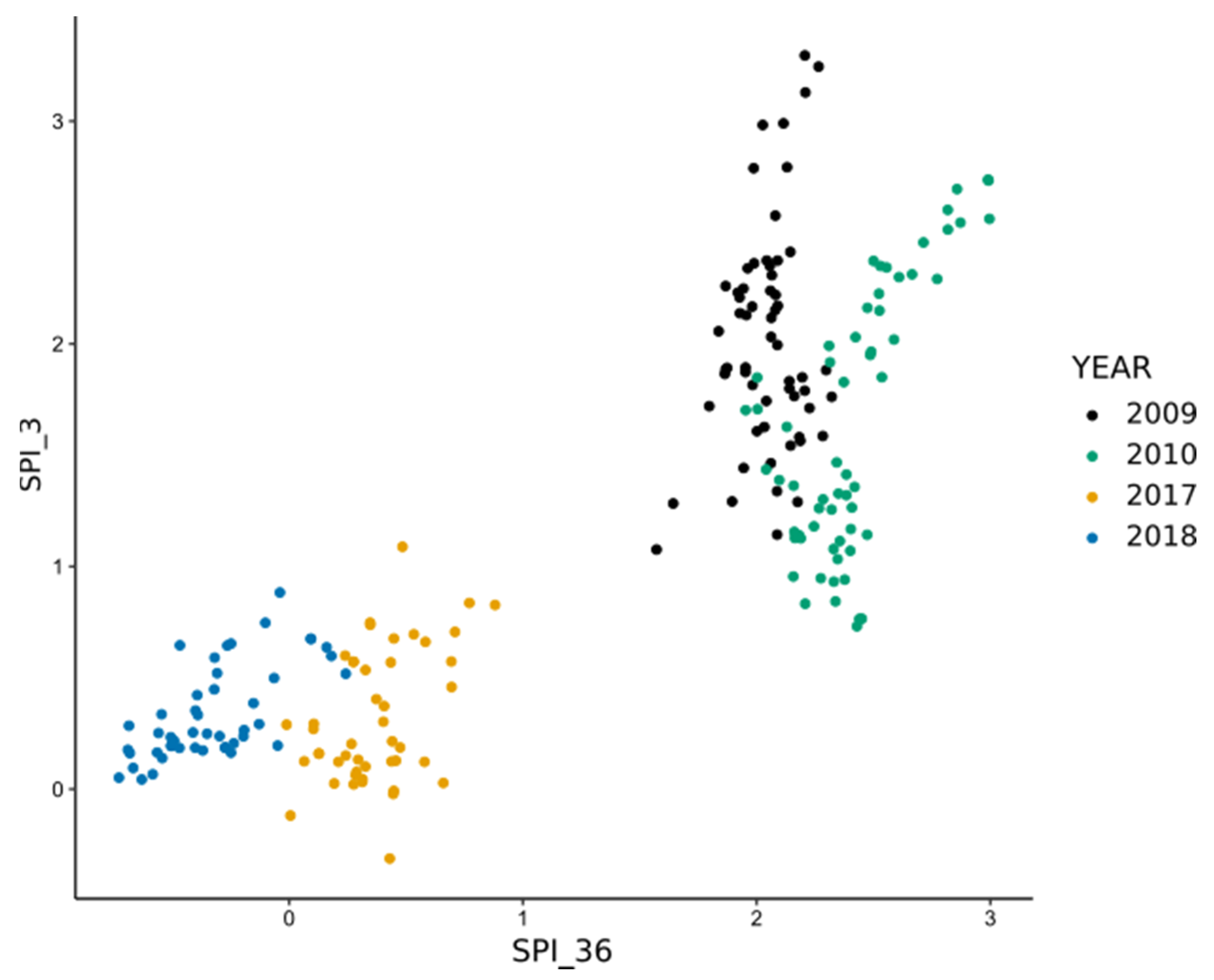
3.1. Characteristics of Vegetation and Climate during the Period of Interest

Rangeland production is generally low in the area with an average value of 0.65 t/ha over the study sites for the four years of interest. It is highly variable as well since maximum values can reach 3 to 3.5 t/ha. The year 2009 was on average the most productive with a mean production of 1.14 t/ha, followed by 2018 (0.65 t/ha), 2017 (0.50 t/ha), and finally 2010 (0.30 t/ha). All years are characterized by highly variable biomass values between the study sites as the standard deviation was of the same order of magnitude as the average value in every case.
The temporal profile of precipitation cumulated over the growing season (September to April) (Figure 3, Figure S2 (for black and white version)) shows that our first period of interest, the 2008–2009 and 2009–2010 seasons (later referred to as 2009 and 2010), is above average (152 mm) in terms of precipitation, with cumulative values of 297 and 230 mm of rainfall, while during the second period of interest in this study (the 2016–2017 and 2017–2018 seasons, later referred to as 2017 and 2018), 2017 was closer to average but still wetter (185 mm) and 2018 was drier than average (129 mm). Relative to the 1982–2019 period, the years 2009 and 2010 were characterized by favorable rainfall conditions for both short and long terms while the year 2017 was drier but still above the reference period, with SPI values between 0 and 1 for accumulation periods of 3 and 36 months (Figure 4, Figure S3 (for black and white version)). The year 2018 was, however, worse off in the long term, with negative values for SPI_36 (Figure 4, Figure S3).

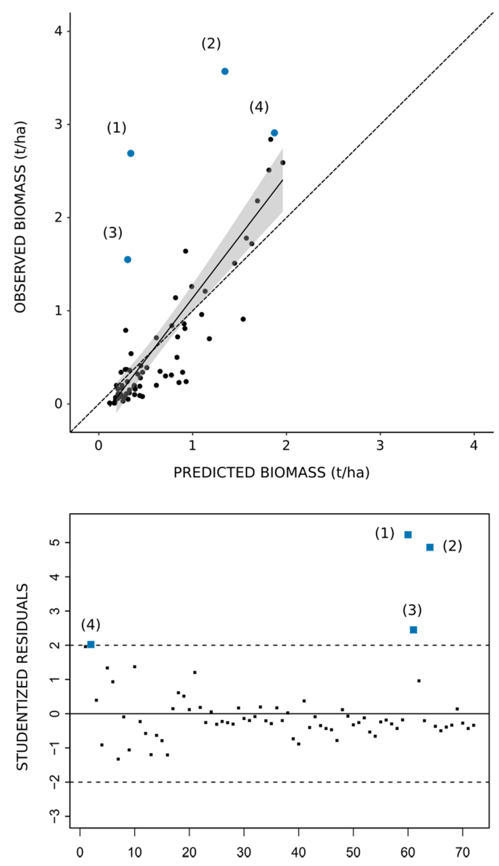
3.2. Global Model for Estimation of Rangeland Biomass

Correlation with biomass was found to be significant, with a p-value < 0.001 for reflectances in the six Landsat 7 ETM+ bands as well as the derived vegetation indices for both linear (Pearson) and monotonic (Spearman) relations (Table 2). For precipitation-related variables, correlation coefficients were inferior to most of the spectral variables (reflectances and VIs) and were found to be non-significant for a majority of them, except for medium to long term accumulation periods (6, 9 and 12 months for Pearson’s coefficient). The highest coefficient of correlation was found for the Atmospherically Resistant Vegetation Index (ARVI), with values of 0.77 and 0.72 for Pearson’s and Spearman’s coefficients.
In the training phase of our procedure, the model built on the calibration sample explains 56% in the response variable (R2 = 0.56) and is characterized by a mean absolute error of 0.32 t/ha (or 52% for the normalized MAE (MAE/mean biomass)) and a root mean square error of 0.46 t/ha (75%) (Table 3). Biomass was predicted using the validation dataset and performance metrics computed in the validation (testing) phase of the model (Table 3) are comparable to those obtained during the training phase with an R2 value of 0.63, a mean absolute error equal to 0.33 t/ha (49%), and a root mean square error of 0.53 t/ha (79%).
In terms of unbiased importance (Table 4), we found that vegetation indices that are ranked the highest are also found to have the highest values of correlation, with the top five variables being in both cases ARVI, NDVI, EVI, TSAVI, and the ratio between the NIR and R reflectances. In the first position, we find the Atmospherically Resistant Vegetation Index (ARVI). A second group is composed of NDVI, EVI, TSAVI, NIR/R, and SIPI, with an importance value equal to 40 to 50% of that of the most important variable. Finally, a third group, characterized by importance values lower than 30% of the importance of ARVI, contains mostly the SPI variables, the simple reflectances, and some of the spectral indices. Regarding spectral indices, we found that seven out of the nine spectral indices involving the R and NIR bands have the highest values of importance, while combinations involving the SWIR bands or simple reflectance are among the least important predictors in the model.
The performance of the rangeland biomass model was further assessed through the comparison of observed and predicted biomass values and the study of residuals (Figure 5, Figure S4 (for black and white version)). The analysis of residuals of the prediction from the validation sample showed that they are not significantly correlated to predicted biomass (r = 0.13, p-value = 0.281). Furthermore, the Shapiro–Wilk test leads us to reject the hypothesis that the residuals are normally distributed (W = 0.74, p-value = 5.627 × 10⁻¹⁰) and a comparison of observed and predicted values (Figure 5, Figure S4) shows a tendency to underestimate biomass (and therefore a distribution of residuals that is heavier on the negative side).
The identification of the largest residuals by the means of studentization of the values (Table 5) shows that four observations in the validation dataset are characterized by a particularly high error (with a studentized value superior to 2). Out of these four observations, three concern samples collected in alfa steppes with high values of biomass (superior to 2 t/ha) compared to the mean observed value in the validation sample (0.67 t/ha).

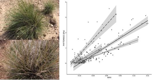
3.3. Linear Relation between Biomass and ARVI

Comparison of the linear relation between biomass and ARVI shows a certain closeness between the linear regression models obtained for all observations (Figure 6, top, Figure S5 (for black and white version), top) and models designed for alfa steppes and other forms of vegetation separately (Figure 6, bottom, Figure S5, bottom), with similar values for the slope and intercept of the three models. Closer inspection of the models’ plots allowed one to highlight the fact that observation points for the alfa steppes spread more around their regression line than for other formations of vegetation. This is reflected in the variations of the values of the coefficient of determination which drops to 0.43 (adjusted value = 0.42) for alfa steppes but increases for other types of vegetation (0.68, adjusted value = 0.67) (Table 6). As a result, we can also observe an increase in metrics values related to the model error for the alfa steppes and lower values for other types of vegetation (Table 6). However, due to a higher yield in alfa steppes (with an average biomass value of 1.09 t/ha), relative values of the error metrics are lower for this vegetation formation. In the model including all vegetation formations, we also detect that the observations with the highest residual values (Table 7) occur mostly for data collected at the alfa sites (six out of eight).
Closer inspection of the linear relationship between biomass and ARVI for the alfa steppe over the years (Figure 7, Figure S6 (for black and white version)) reveals certain disparities between the years, especially concerning the slope of the model (Table 8), which is multiplied by a factor of 2.5 between its lowest and highest values, and the performance metrics (Table 9), highlighting the year 2010 as the best year in terms of R2 and error values.

4. Discussion

This study aimed at investigating the potential of vegetation indices and precipitation-related variables derived from remote sensing to assess rangeland production in the arid environment of the Moroccan Oriental region and identify the challenges linked to that particular biome.
Results of the correlation analysis (Table 2) proved the potential of spectral reflectances and indices to estimate the production of rangelands in the Moroccan Oriental and justified their integration into a Random Forest model for biomass prediction. In the global model, correlations were found significant for all the spectral reflectances and VIs with absolute values ranging from 0.36 to 0.77. Five of the fourteen indices have a correlation to biomass above 0.70 and among them, the three best, namely ARVI, the ratio of NIR to R and NDVI, individually explain more than 50% of the variations in biomass (with corresponding R2 values of 0.59, 0.53 and 0.52). These results can be considered average for this type of biome, as similar values are found for models including a single index in the Sahel by [28] (R2 = 0.68 for NDVI in Senegal) and [29] (R2 = 0.47 for NDVI cumulated over the growing season in Niger); in the arid regions of the United States with R2 equal or inferior to 0.40 for various VIs (including 0.28 for NDVI) in Idaho [33]; across Australia, where low R2 values were observed for a global model (below 0.2 for a series of vegetation indices) [35]; while in Iran, reference [36], recorded a coefficient of determination between above-ground biomass and NDVI equal to 0.57, reference [37] observed correlations between NDVI and rangeland production ranging from 0.55 to 0.88 (corresponding to R2 values of 0.30 to 0.75) depending on the dominant species, and reference [38] computed a pseudo-R2 ranging from 0.02 (EVI) to 0.33 (NDVI) and 0.47 (Transformed NDVI). Besides, a review paper on the use of remote sensing for grassland management [17] mentions values of R2 varying from 0.40 to 0.97.
In terms of variable ranking, for both correlation (Table 2) and conditional permutation importance (Table 4), we found that vegetation indices that scored best involve a combination of the R and NIR bands while spectral reflectances and indices built on other bands are found to be of weak importance in the prediction of rangeland biomass. Indices with built-in atmospheric correction (provided by the blue band) were also of interest in the global model, especially ARVI, which was ranked first for both correlation and importance. On the other hand, indices including the SWIR bands performed worse at predicting rangeland biomass in the global model than VIs based on the R and NIR bands. This result was unexpected, as water plays a significant role in the development of vegetation in the arid regions and other studies found that water-stress-related indices performed better at estimating biomass. For example, we can note [34], for which NDVI and SAVI were not correlated to biomass while significant R2 values were found for NDWI built on Landsat’s SWIR bands; [33], which found better correlation when the SWIR band was substituted to the R band in traditional VIs; [40], for which NDWI was considered as an important variable, and [32], which also observed that vegetation indices built on the SWIR bands outperformed NDVI, SAVI, and MSAVI. This behavior could be explained by several factors, including confusion between plant and soil water content in areas characterized by a low percentage of vegetation cover, and a high proportion of senescent vegetation, whose spectrum is more similar to that of the soil [88], causing a less pronounced contrast between reflectances in the NIR and SWIR bands than for green vegetation.
Additionally, in the family of Soil-Adjusted Vegetation Indices, we found that SAVI performed the poorest. We attribute this to the lack of flexibility introduced by the L factor that was kept constant for all observations. Indeed, while the percent of canopy cover is low in general (15% on average) and justifies an L value of one, its distribution also spreads towards increasing values, with percent cover even reaching 50% depending on the year and vegetation formation. Although MSAVI was designed to self-adjust to unknown fractions of vegetation cover, it did not perform well in terms of variable importance. While TSAVI performed better than any other index in the Soil-Adjusted Vegetation Indices, it did not improve the prediction of biomass in the global model compared to indices without a soil adjustment factor. This effect could again be explained by a large fraction of senescent vegetation which could cause confusion between vegetation and soil signal, since information received in the R and NIR channels that are involved in the self-adjusted factor is similar for vegetation and soil.
Correlation analysis also revealed that precipitation-related variables were poorly, and even not, in certain cases, correlated to biomass, with the strongest relationship happening for an accumulation period of 6 months (R = 0.35 and 0.41 for Pearson and Spearman coefficients), followed by two other medium to long-term accumulation periods (9 and 12 months). These results are consistent with the fact that perennial vegetation constitutes a large fraction of the vegetation in the area and that medium to long-term accumulation periods better reflect the growth cycle of the plants. SPI_6 (and, to a lesser extent, SPI_9 and SPI_12) reflects the rainfall conditions during the growing period and includes, for example for alfa steppes, the fall months (October to December), which constitutes an active period of growth, while shorter accumulation periods mostly contain the winter months (January to March) where growth slows down [89]. The poor predictive power of rainfall-related variables could partially be explained by the coarse resolution of the precipitation data (0.05°) which may not accurately represent the local conditions in this region characterized by spatially variable rainfall but also to the more complex relationship between biomass production and rainfall in areas covered in majority by perennial species.
Despite their poor correlation to biomass, SPI variables were added to the random forest model to take into account possible interactions between the spectral and rainfall-related predictors in the assessment of biomass (as it was observed by [27,28,90]). Still, such interactions were not detected in the design of the global Random Forest model since SPI variables were found to be of low importance. Their impact on the accuracy of the assessment of rangeland biomass has, however, not been fully characterized, as no comparison was realized between models based solely on vegetation indices and models combining VIs and SPI.
Integration of all the variables in a Random Forest model only slightly improved the predictive power compared to the use of single indices as the coefficient of determination increased to 0.63 (Table 3). In other studies [31,35], an improvement in the metrics was observed when comparing the performance of simple and multi-linear models in assessing vegetation biomass in arid regions. Even though consistency between calibration and validation metrics demonstrated that our model is stable and able to predict biomass for a new dataset, it is also characterized by a moderate coefficient of determination (R2 = 0.63) and a high error value in relative terms (49% for MAE and 79% for RMSE for the validation dataset) (Table 3). The absolute value of RMSE (0.53 t/ha) is, however, of the same order of magnitude as the values obtained by [39] (0.63 and 0.79 t/ha, or 42 and 53% in relative values, for their artificial neural network and multi-linear regression), [29] (0.45 t/ha in the case of their global model), [40] (ranging from 0.73 to 0.99 t/ha depending on vegetation type and with a value of 0.77 t/ha for their global model) and [32] (0.80 and 0.69 t/ha for their simple linear and support vector machine models when all observations are pooled). Analysis of the residuals (Figure 5, Figure S4, Table 5) revealed that the most important source of error in the prediction of rangeland biomass was due to the presence of alfa steppes, a vegetation formation dominated by Stipa tenacissima, a perennial herbaceous species of the Poaceae family. Indeed, most of the high residual observations in the validation sample occurred for this particular vegetation formation and areas characterized by a high value of rangeland biomass compared to the average value.
The output of the global model led us to investigate in more depth the relationship between vegetation indices and biomass for the different types of vegetation cover. In particular, we compared linear regressions between the Atmospherically Resistant Vegetation Index, which was found to be the best predictor in terms of permutation-based importance, and biomass between different vegetation formation groups (all forms pooled, alfa steppes alone and other vegetation formations pooled). Although no considerable difference was found between the three linear models’ equations (similar values for slope and intercept), scatterplots of biomass versus ARVI allowed us to detect that observations collected on alfa sites spread more around their regression line than for other formations of vegetation, causing an increase in error when these points are associated to other formations of vegetation in the model (Figure 6, Figure S5). This fact is consistent with the analysis of residuals performed for the global Random Forest model (Table 5) as well as the linear model (Table 7) where we uncovered that the highest residuals were found to be mostly linked to alfa steppes. A poorer (and even non-significant) correlation between biomass and VIs was also observed for another species of the Poaceae family [35].
In our study, correlation and variable importance showed that indices that were designed to reduce the influence of the soil background in the signal (the SAVI family) do not perform better than others at predicting rangeland biomass. Moreover, we found that the highest source of error was linked to a particular plant species. This demonstrates that, in the case of the Moroccan Oriental region, the particularities of Stipa tenacissima are the largest cause of error when assessing rangeland biomass from vegetation indices and that the use of a global model is therefore not advised in the area. Furthermore, analysis of the residuals exposed a systematic underestimation of rangeland biomass for alfa sites characterized by a high value of biomass (Table 5). Indeed, the highest values of prediction error were all found to be positive (i.e., the predicted value was inferior to the observed one) and were observed for sites presenting high biomass compared to the average value. Besides, both the analysis of residuals and the study of the linear relation between alfa steppes biomass and ARVI for individual years revealed the disparities between the years, both in terms of model parameters (slope) (Figure 7, Figure S6, Table 8) and performance (Table 9). While performance metrics showed that model performance varied between the years, models’ equations highlighted the changes in sensitivity of ARVI to variations of biomass as a function of the year. Figure 7 and Figure S6 particularly highlight the fact that, even though alfa biomass exhibits a large range of variation for 2018, it is associated with limited variation in ARVI, while the opposite can be observed for the year 2010 and, to a lesser extent, 2009. In [27,28], such differences were also observed in R2 values and parameters of the regression lines between the years in Senegal, which were attributed to inter-annual variations in atmospheric conditions. Similarly, in Australia, VIs were found to perform differently at capturing the variations in canopy cover between the years but also between the study sites and the study concludes that the variability of rainfall adds a level of difficulty in the monitoring of the vegetation cover [87]. In the arid and semi-arid regions of Morocco for our period of interest, the difference between the years for which the study was carried out also translates in different meteorological conditions, mainly in terms of rainfall and its effect in the short and long term. While in the early years of the study (2009 and 2010) we observed good conditions with regard to precipitation, the later years (2017 and 2018) were stricken by drier conditions in both the short and long term.
In the case of perennial herbaceous species, while in good rainfall conditions, the plant grows and more green matter is produced, the accumulation of dry conditions over the years translates into a build-up of dry, non-photosynthetic material. In the Oriental region, this effect is particularly important for Stipa tenacissima and is clearly visible when comparing the greenness of two alfa plants from sites located in close vicinity of each other (about 1 km) for the years 2009 and 2018 (Figure 8). These two examples illustrate the impact of the accumulation of dry, non-photosynthetic, vegetation after a long period of unfavorable rainfall on the sensitivity of ARVI to changes in biomass. Indeed, for these sites, while rangeland biomass is higher in 2018 (3.19 t/ha versus 2.18 t/ha in 2009), it does not translate in a linear increase in ARVI between 2009 and 2018 since we measured similar median values (0.04 and 0.06) over the 2018 and 2009 sites.
A second effect, linked to the number of annual plants, superimposes on the influence of variations in the greenness of alfa in the ARVI response to changes in rangeland biomass. Indeed, during wet years, a greater quantity of green, annual plants is present in the study sites, which further increases the sensitivity of the ARVI. It was the case in the 2009 and 2010 campaigns, where a large quantity of healthy annual vegetation increased both the biomass and greenness of the region’s rangeland, while in the spring of 2017 and 2018, a very limited amount of green annual plants was observed on the field, therefore further increasing the proportion of non-photosynthetic vegetation and in consequence, diminishing the ability of ARVI to assess the total rangeland biomass.
As a first step toward the improvement of the prediction of rangeland biomass in the Oriental, we suggest treating the case of alfa steppes separately from the other forms of vegetation. A methodology to map rangeland cover based on Landsat images and prior knowledge on geology and climate knowledge was developed in the Oriental [16]. It was successful at discriminating alfa steppes (kappa coefficient = 95%) and can therefore be used to effectively partition our study area. In the particular case of alfa steppes, we recommend focusing on methods dedicated to the discrimination of green vegetation, non-photosynthetic vegetation, and bare soil. Furthermore, even though interactions between vegetation indices and precipitation-related variables were not detected by the global Random Forest model, they were observed in the study of the relationship between ARVI and alfa steppes biomass over time, as the repeated occurrence of drier periods causes an accumulation of non-photosynthetic material in the plants. We therefore recommend looking deeper into the short and long-term effects of precipitation on the development of vegetation in alfa steppes and the relation between vegetation indices and rangeland biomass.
For other forms of vegetation, we recommend the in-depth examination of the relationship between rangeland biomass and vegetation indices the same way it was realized for the global model and the case of alfa steppes to properly assess their potential and possible ways of improvement.
Although the Random Forest model did not perform much better than the simple linear model, we do not attribute this to limitations in the algorithm but rather to the limitations of our study, i.e., the fact that the VIs used here are unsuited to estimate biomass in the Oriental due to the large proportion of non-photosynthetic vegetation and recommend to continue using this algorithm, as it is suited for complex non-linear phenomena such as biomass estimation. In addition, when building Random Forest models for biomass prediction, the selection of appropriate variables based on the values of importance might also further increase the performance of the model compared to a model including all the variables, as it is the case for the current global model.

5. Conclusions

A global model including remote sensing spectral vegetation indices and precipitation-related variables was tested to assess rangeland biomass in the arid region of the Moroccan Oriental. Although some individual VIs showed promising potential for the prediction of biomass, the performance of the model remained limited with a moderate value of R2 and a high relative error. Our analysis of the global model output and after that, of the relationship between biomass and the Atmospherically Resistant Vegetation Index for the different vegetation formations and over time, led us to the conclusion that, in the case of the Oriental, the presence of alfa steppes dominated by Stipa tenacissima causes a decrease in the quality of the prediction and that a global model is therefore not suited to assess rangeland biomass. Vegetation in arid and semi-arid regions is characterized by the presence of non-photosynthetic vegetation, whose spectrum diverges from that of the green vegetation. In the case of Stipa tenacissima, the tussocks can contain a large fraction of senescent leaves, which particularly affects the ability of classical vegetation indices to predict plant biomass by disturbing the signal emitted by the vegetation, especially in the red and infrared regions.
We suggest treating the case of alfa steppes separately from the other forms of vegetation in further studies. For alfa steppes, we recommend focusing on methods dedicated to the discrimination of green vegetation, non-photosynthetic vegetation, and bare soil and to investigate in more detail the relationship between precipitation (in the short and long term) and plant growth and their impact on vegetation indices.
Finally, this study also demonstrated the importance of the validation of vegetation indices by in situ measurements before they can be used to monitor the spatial and temporal variations of vegetation properties. Indeed, results obtained in the arid and semi-arid regions of Morocco showed that the variations in biomass are not uniformly reflected in the variations of the vegetation indices. Especially in the case of alfa steppes, the large proportion of senescent vegetation caused a decrease in the values of the VIs during the drier years (2017 and 2018) that could have been incorrectly interpreted as a reduction in rangeland production without comparison to ground measurements.

Supplementary Materials

The following are available online at https://www.mdpi.com/article/10.3390/rs13112093/s1, Figure S1: soil line in the NIR vs. R space (line = quantile regression with tau = 2 × 10⁻³), Figure S2: evolution of precipitation (mm) from 1982 to 2019 over the Oriental. Bars = cumulated precipitation over the year and the growing season (growing season i = September of year i − 1 to March of year i). Lines = 1982–2019 average for annual and growing season precipitation. Data: CHIRPS v2.0 [81]., Figure S3: short-term (SPI_3) and long-term (SPI_36) precipitation conditions over the study sites in 2009, 2010, 2017, and 2018, Figure S4: relationship between observed and predicted biomass values (top), and studentized residuals (bottom) for the validation sample. 1 to 4: observations characterized by a value of studentized residuals outside the [−2, 2] interval (identification of observations in Table 5). Top panel: solid line = linear fit, grey area = 95% confidence interval on the regression line, dashed line= Y = X, Figure S5: comparison of the linear relation between biomass and ARVI for the overall case (top) and alfa steppes vs. other types of vegetation formation (bottom). Solid and dashed lines = linear regression, grey area = 95% confidence interval on the regression line, Figure S6: comparison of the linear relation between alfa steppes biomass and ARVI for the years 2009, 2010, 2017, and 2018. Solid and dashed lines = linear regression, grey area = 95% confidence interval on the regression line.

Author Contributions

Conceptualization, M.L., H.M., and B.T.; methodology, M.L., H.M., and B.T.; software, M.L.; validation, M.L.; formal analysis, M.L.; investigation, M.L.; resources, M.L., H.M., and B.T.; data curation, M.L., and H.M.; writing—original draft preparation, M.L.; writing—review and editing, M.L., H.M., and B.T.; visualization, M.L.; supervision, M.L., H.M., and B.T.; project administration, M.L., H.M., and B.T.; funding acquisition, M.L., H.M., and B.T. All authors have read and agreed to the published version of the manuscript.

Funding

This research received no external funding.

Institutional Review Board Statement

Not applicable.

Informed Consent Statement

Not applicable.

Data Availability Statement

Not applicable.

Acknowledgments

The authors would like to thank Azeddine Hachmi for the organization of the data collection campaign of 2017 and 2018.

Conflicts of Interest

The authors declare no conflict of interest.

References

  1. Middleton, N.; Thomas, D.S.G. World Atlas of Desertification, 2nd ed.; Arnold: London, UK; John Wiley: Hoboken, NJ, USA, 1997. [Google Scholar]
  2. Weber, K.T.; Horst, S. Desertification and Livestock Grazing: The Roles of Sedentarization, Mobility and Rest. Pastor Res Policy Pract. 2011, 1, 19. [Google Scholar] [CrossRef] [Green Version]
  3. Scholes, R.J. The Future of Semi-Arid Regions: A Weak Fabric Unravels. Climate 2020, 8, 43. [Google Scholar] [CrossRef] [Green Version]
  4. Safriel, U.; Adeel, Z.; Niemeijer, D.; Puigdefabregas, J.; White, R.; Lal, R.; Winslow, M.; Ziedler, J.; Prince, S.; Archer, E.; et al. Dryland Systems. In Global Assessment Reports Volume 1: Current State and Trends; Millennium Ecosystem Assessment; Island Press: Washington, DC, USA, 2005. [Google Scholar]
  5. Huang, J.; Ji, M.; Xie, Y.; Wang, S.; He, Y.; Ran, J. Global Semi-Arid Climate Change over Last 60 Years. Clim. Dyn. 2016, 46, 1131–1150. [Google Scholar] [CrossRef] [Green Version]
  6. Eisfelder, C.; Kuenzer, C.; Dech, S. Derivation of Biomass Information for Semi-Arid Areas Using Remote-Sensing Data. Int. J. Remote Sens. 2012, 33, 2937–2984. [Google Scholar] [CrossRef]
  7. Dong, S. Overview: Pastoralism in the World. In Building Resilience of Human-Natural Systems of Pastoralism in the Developing World; Dong, S., Kassam, K.-A.S., Tourrand, J.F., Boone, R.B., Eds.; Springer International Publishing: Cham, Switzerland, 2016; pp. 1–38. ISBN 978-3-319-30730-5. [Google Scholar]
  8. Rishmawi, K.; Prince, S.; Xue, Y. Vegetation Responses to Climate Variability in the Northern Arid to Sub-Humid Zones of Sub-Saharan Africa. Remote Sens. 2016, 8, 910. [Google Scholar] [CrossRef] [Green Version]
  9. Sloat, L.L.; Gerber, J.S.; Samberg, L.H.; Smith, W.K.; Herrero, M.; Ferreira, L.G.; Godde, C.M.; West, P.C. Increasing Importance of Precipitation Variability on Global Livestock Grazing Lands. Nat. Clim Chang. 2018, 8, 214–218. [Google Scholar] [CrossRef]
  10. Godde, C.; Dizyee, K.; Ash, A.; Thornton, P.; Sloat, L.; Roura, E.; Henderson, B.; Herrero, M. Climate Change and Variability Impacts on Grazing Herds: Insights from a System Dynamics Approach for Semi-arid Australian Rangelands. Glob Chang. Biol 2019, 25, 3091–3109. [Google Scholar] [CrossRef] [Green Version]
  11. IPCC. Climate Change 2013: The Physical Science Basis; Stocker, T.F.D., Qin, G.-K., Plattner, M., Tignor, S.K., Allen, J., Boschung, A., Nauels, Y., Xia, V.B., Midgley, P.M., Eds.; Contribution of Working Group I to the Fifth Assessment Report of the Intergovernmental Panel on Climate Change; Cambridge University Press: Cambridge, UK; New York, NY, USA, 2013. [Google Scholar]
  12. Food and Agriculture Organization of the United Nations. Pastoralism in Africa’s Drylands: Reducing Risks, Addressing Vulnerability and Enhancing Resilience; FAO: Rome, Italy, 2018. [Google Scholar]
  13. Koocheki, A.; Gliessman, S.R. Pastoral Nomadism, a Sustainable System for Grazing Land Management in Arid Areas. J. Sustain. Agric. 2005, 25, 113–131. [Google Scholar] [CrossRef]
  14. Boutaleb, A.; Firmian, I. Community Governance Of Natural Resources And Rangelands: The Case Of The Eastern Highlands Of Morocco. In The Governance of Rangelands—Collective Action for Sustainable Pastoralism; Routledge: London, UK, 2014; pp. 94–107. ISBN 978-1-315-76801-4. [Google Scholar]
  15. Dong, S.; Liu, S.; Wen, L. Vulnerability and Resilience of Human-Natural Systems of Pastoralism Worldwide. In Building Resilience of Human-Natural Systems of Pastoralism in the Developing World; Dong, S., Kassam, K.-A.S., Tourrand, J.F., Boone, R.B., Eds.; Springer International Publishing: Cham, Switzerland, 2016; pp. 39–92. ISBN 978-3-319-30730-5. [Google Scholar]
  16. Mahyou, H.; Tychon, B.; Balaghi, R.; Louhaichi, M.; Mimouni, J. A Knowledge-Based Approach for Mapping Land Degradation in the Arid Rangelands of North Africa: Mapping Land Degradation in the Arid Rangelands. Land Degrad. Dev. 2016, 27, 1574–1585. [Google Scholar] [CrossRef]
  17. Reinermann, S.; Asam, S.; Kuenzer, C. Remote Sensing of Grassland Production and Management—A Review. Remote Sens. 2020, 12, 1949. [Google Scholar] [CrossRef]
  18. Tucker, C.J. Red and Photographic Infrared Linear. Combinations for Monitoring Vegetation. Remote Sens. Environ. 1979, 8, 127–150. [Google Scholar] [CrossRef] [Green Version]
  19. Huete, A.; Didan, K.; Miura, T.; Rodriguez, E.P.; Gao, X.; Ferreira, L.G. Overview of the Radiometric and Biophysical Performance of the MODIS Vegetation Indices. Remote Sens. Environ. 2002, 83, 195–213. [Google Scholar] [CrossRef]
  20. Huete, A.R. A Soil-Adjusted Vegetation Index (SAVI). Remote Sens. Environ. 1988, 25, 295–309. [Google Scholar] [CrossRef]
  21. Baret, F.; Guyot, G.; Major, D.J. TSAVI: A Vegetation Index Which Minimizes Soil Brightness Effects On LAI And APAR Estimation. In Proceedings of the 12th Canadian Symposium on Remote Sensing Geoscience and Remote Sensing Symposium, Vancouver, BC, Canada, 10–14 July 1989; Volume 3, pp. 1355–1358. [Google Scholar]
  22. Qi, J.; Chehbouni, A.; Huete, A.R.; Kerr, Y.H.; Sorooshian, S. A Modified Soil Adjusted Vegetation Index. Remote Sens. Environ. 1994, 48, 119–126. [Google Scholar] [CrossRef]
  23. Rondeaux, G.; Steven, M.; Baret, F. Optimization of Soil-Adjusted Vegetation Indices. Remote Sens. Environ. 1996, 55, 95–107. [Google Scholar] [CrossRef]
  24. Hatfield, J.L.; Prueger, J.H.; Sauer, T.J.; Dold, C.; O’Brien, P.; Wacha, K. Applications of Vegetative Indices from Remote Sensing to Agriculture: Past and Future. Inventions 2019, 4, 71. [Google Scholar] [CrossRef] [Green Version]
  25. Ali, I.; Cawkwell, F.; Dwyer, E.; Barrett, B.; Green, S. Satellite Remote Sensing of Grasslands: From Observation to Management. J. Plant Ecol. 2016, 9, 649–671. [Google Scholar] [CrossRef] [Green Version]
  26. Baret, F.; Guyot, G. Potentials and Limits of Vegetation Indices for LAI and APAR Assessment. Remote Sens. Environ. 1991, 35, 161–173. [Google Scholar] [CrossRef]
  27. Diallo, O.; Diouf, A.; Hanan, N.P.; Ndiaye, A.; Prévost, Y. AVHRR Monitoring of Savanna Primary Production in Senegal, West Africa: 1987–1988. Int. J. Remote Sens. 1991, 12, 1259–1279. [Google Scholar] [CrossRef]
  28. Diouf, A.; Lambin, E.F. Monitoring Land-Cover Changes in Semi-Arid Regions: Remote Sensing Data and Field Observations in the Ferlo, Senegal. J. Arid Environ. 2001, 48, 129–148. [Google Scholar] [CrossRef]
  29. Schucknecht, A.; Meroni, M.; Kayitakire, F.; Boureima, A. Phenology-Based Biomass Estimation to Support Rangeland Management in Semi-Arid Environments. Remote Sens. 2017, 9, 463. [Google Scholar] [CrossRef] [Green Version]
  30. Mahyou, H.; Tychon, B.; Lang, M.; Balaghi, R. Phytomass Estimation Using EMODIS NDVI and Ground Data in Arid Rangelands of Morocco. Afr. J. Range Forage Sci. 2018, 35, 1–12. [Google Scholar] [CrossRef]
  31. Mahyou, H. Estimation de la production fourragère des terres de parcours des hauts plateaux de l’oriental (Maroc) par les indices de télédétection. Afr. Mediterr. Agric. Res. J. Al-Awamia 2020, 19, 128. [Google Scholar]
  32. Benseghir, L.; Bachari, N.E.I. Shortwave Infrared Vegetation Index-Based Modelling for Aboveground Vegetation Biomass Assessment in the Arid Steppes of Algeria. Afr. J. Range Forage Sci. 2021, 1–10. [Google Scholar] [CrossRef]
  33. Chen, F.; Weber, K.T.; Gokhale, B. Herbaceous Biomass Estimation from SPOT 5 Imagery in Semiarid Rangelands of Idaho. Giscience Remote Sens. 2011, 48, 195–209. [Google Scholar] [CrossRef]
  34. Numata, I.; Roberts, D.A.; Chadwick, O.A.; Schimel, J.; Sampaio, F.R.; Leonidas, F.C.; Soares, J.V. Characterization of Pasture Biophysical Properties and the Impact of Grazing Intensity Using Remotely Sensed Data. Remote Sens. Environ. 2007, 109, 314–327. [Google Scholar] [CrossRef]
  35. Mundava, C.; Helmholz, P.; Schut, A.G.T.; Corner, R.; McAtee, B.; Lamb, D.W. Evaluation of Vegetation Indices for Rangeland Biomass Estimation in the Kimberley Area of Western Australia. ISPRS Ann. Photogramm. Remote Sens. Spat. Inf. Sci. 2014, II–7, 47–53. [Google Scholar] [CrossRef] [Green Version]
  36. Pordel, F.; Ebrahimi, A.; Azizi, Z. Canopy Cover or Remotely Sensed Vegetation Index, Explanatory Variables of above-Ground Biomass in an Arid Rangeland, Iran. J. Arid Land 2018, 10, 767–780. [Google Scholar] [CrossRef] [Green Version]
  37. Hadian, F.; Jafari, R.; Bashari, H.; Tarkesh, M.; Clarke, K.D. Effects of Drought on Plant Parameters of Different Rangeland Types in Khansar Region, Iran. Arab. J. Geosci 2019, 12, 93. [Google Scholar] [CrossRef]
  38. Gholami Baghi, N.; Oldeland, J. Do Soil-Adjusted or Standard Vegetation Indices Better Predict above Ground Biomass of Semi-Arid, Saline Rangelands in North-East Iran? Int. J. Remote Sens. 2019, 40, 8223–8235. [Google Scholar] [CrossRef]
  39. Xie, Y.; Sha, Z.; Yu, M.; Bai, Y.; Zhang, L. A Comparison of Two Models with Landsat Data for Estimating above Ground Grassland Biomass in Inner Mongolia, China. Ecol. Model. 2009, 220, 1810–1818. [Google Scholar] [CrossRef]
  40. John, R.; Chen, J.; Giannico, V.; Park, H.; Xiao, J.; Shirkey, G.; Ouyang, Z.; Shao, C.; Lafortezza, R.; Qi, J. Grassland Canopy Cover and Aboveground Biomass in Mongolia and Inner Mongolia: Spatiotemporal Estimates and Controlling Factors. Remote Sens. Environ. 2018, 213, 34–48. [Google Scholar] [CrossRef]
  41. Otgonbayar, M.; Atzberger, C.; Chambers, J.; Damdinsuren, A. Mapping Pasture Biomass in Mongolia Using Partial Least Squares, Random Forest Regression and Landsat 8 Imagery. Int. J. Remote Sens. 2019, 40, 3204–3226. [Google Scholar] [CrossRef]
  42. Kaufman, Y.J.; Tanre, D. Atmospherically Resistant Vegetation Index (ARVI) for EOS-MODIS. IEEE Trans. Geosci. Remote Sens. 1992, 30, 261–270. [Google Scholar] [CrossRef]
  43. Huete, A.; Justice, C.; Liu, H. Development of Vegetation and Soil Indices for MODIS-EOS. Remote Sens. Environ. 1994, 49, 224–234. [Google Scholar] [CrossRef]
  44. Penuelas, J.; Baret, F.; Filella, I. Semi-Empirical Indices to Assess Carotenoids/Chlorophyll a Ratio from Leaf Spectral Reflectance. Photosynthetica. 1995, 31, 221–230. [Google Scholar]
  45. Marticorena, B.; Bergametti, G. Modeling the Atmospheric Dust Cycle: 1. Design of a Soil-derived Dust Emission Scheme. J. Geophys. Res. 1995, 100, 16415–16430. [Google Scholar] [CrossRef] [Green Version]
  46. Tegen, I.; Schepanski, K. The Global Distribution of Mineral Dust. Iop Conf. Ser. Earth Environ. Sci. 2009, 7, 012001. [Google Scholar] [CrossRef]
  47. Gao, B. NDWI—A Normalized Difference Water Index for Remote Sensing of Vegetation Liquid Water from Space. Remote Sens. Environ. 1996, 58, 257–266. [Google Scholar] [CrossRef]
  48. Lotsch, A.; Friedl, M.A.; Anderson, B.T.; Tucker, C.J. Coupled Vegetation-Precipitation Variability Observed from Satellite and Climate Records: Vegetation-Precipitation Dynamics. Geophys. Res. Lett. 2003, 30. [Google Scholar] [CrossRef]
  49. Vicente-Serrano, S.M. Evaluating the Impact of Drought Using Remote Sensing in a Mediterranean, Semi-Arid Region. Nat. Hazards 2007, 40, 173–208. [Google Scholar] [CrossRef]
  50. Sierra-Soler, A.; Adamowski, J.; Malard, J.; Qi, Z.; Saadat, H.; Pingale, S. Assessing Agricultural Drought at a Regional Scale Using LULC Classification, SPI, and Vegetation Indices: Case Study in a Rainfed Agro-Ecosystem in Central Mexico. Geomat. Nat. Hazards Risk 2016, 7, 1460–1488. [Google Scholar] [CrossRef] [Green Version]
  51. Hua, L.; Wang, H.; Sui, H.; Wardlow, B.; Hayes, M.J.; Wang, J. Mapping the Spatial-Temporal Dynamics of Vegetation Response Lag to Drought in a Semi-Arid Region. Remote Sens. 2019, 11, 1873. [Google Scholar] [CrossRef] [Green Version]
  52. Reddy, G.P.O.; Kumar, N.; Sahu, N.; Srivastava, R.; Singh, S.K.; Naidu, L.G.K.; Chary, G.R.; Biradar, C.M.; Gumma, M.K.; Reddy, B.S.; et al. Assessment of Spatio-Temporal Vegetation Dynamics in Tropical Arid Ecosystem of India Using MODIS Time-Series Vegetation Indices. Arab. J. Geosci. 2020, 13, 704. [Google Scholar] [CrossRef]
  53. Nandintsetseg, B.; Shinoda, M. Assessment of Drought Frequency, Duration, and Severity and Its Impact on Pasture Production in Mongolia. Nat. Hazards 2013, 14, 995–1008. [Google Scholar] [CrossRef]
  54. Diouf, A.; Hiernaux, P.; Brandt, M.; Faye, G.; Djaby, B.; Diop, M.; Ndione, J.; Tychon, B. Do Agrometeorological Data Improve Optical Satellite-Based Estimations of the Herbaceous Yield in Sahelian Semi-Arid Ecosystems? Remote Sens. 2016, 8, 668. [Google Scholar] [CrossRef] [Green Version]
  55. McKee, T.B.; Doesken, N.J.; Kleist, J. The Relationship Of Drought Frequency And Duration To Time Scales. In Proceedings of the Eighth Conference on Applied Climatology, Anaheim, CA, USA, 17–22 January 1993. [Google Scholar]
  56. Edwards, D.C. Characteristics of 20th Century Drought in the United States at Multiple Time Scales. Master’s Thesis, Colorado State University, Fort Collins, CO, USA, 1997. [Google Scholar]
  57. Horion, S.; Carrão, H.; Singleton, A.; Barbosa, P.; Vogt, J. JRC Experience on the Development of Drought Information Systems: Europe, Africa and Latin America; Publications Office of the European Union: Luxembourg, 2012. [Google Scholar] [CrossRef]
  58. World Meteorological Organization. Standardized Precipitation Index User Guide; World Meteorological Organization: Geneva, Switzerland, 2012; ISBN 978-92-63-11091-6. [Google Scholar]
  59. Liu, L.; Zhang, Y.; Wu, S.; Li, S.; Qin, D. Water Memory Effects and Their Impacts on Global Vegetation Productivity and Resilience. Sci. Rep. 2018, 8, 2962. [Google Scholar] [CrossRef]
  60. Guerschman, J.P.; Hill, M.J.; Leys, J.; Heidenreich, S. Vegetation Cover Dependence on Accumulated Antecedent Precipitation in Australia: Relationships with Photosynthetic and Non-Photosynthetic Vegetation Fractions. Remote Sens. Environ. 2020, 240, 111670. [Google Scholar] [CrossRef]
  61. Verrelst, J.; Camps-Valls, G.; Muñoz-Marí, J.; Rivera, J.P.; Veroustraete, F.; Clevers, J.G.P.W.; Moreno, J. Optical Remote Sensing and the Retrieval of Terrestrial Vegetation Bio-Geophysical Properties—A Review. ISPRS J. Photogramm. Remote Sens. 2015, 108, 273–290. [Google Scholar] [CrossRef]
  62. Ali, I.; Greifeneder, F.; Stamenkovic, J.; Neumann, M.; Notarnicola, C. Review of Machine Learning Approaches for Biomass and Soil Moisture Retrievals from Remote Sensing Data. Remote Sens. 2015, 7, 16398–16421. [Google Scholar] [CrossRef] [Green Version]
  63. Weiss, M.; Jacob, F.; Duveiller, G. Remote Sensing for Agricultural Applications: A Meta-Review. Remote Sens. Environ. 2020, 236, 111402. [Google Scholar] [CrossRef]
  64. Zhu, X.X.; Tuia, D.; Mou, L.; Xia, G.-S.; Zhang, L.; Xu, F.; Fraundorfer, F. Deep Learning in Remote Sensing: A Comprehensive Review and List of Resources. IEEE Geosci. Remote Sens. Mag. 2017, 5, 8–36. [Google Scholar] [CrossRef] [Green Version]
  65. Ma, L.; Liu, Y.; Zhang, X.; Ye, Y.; Yin, G.; Johnson, B.A. Deep Learning in Remote Sensing Applications: A Meta-Analysis and Review. ISPRS J. Photogramm. Remote Sens. 2019, 152, 166–177. [Google Scholar] [CrossRef]
  66. Ball, J.E.; Anderson, D.T.; Chan, C.S. Comprehensive Survey of Deep Learning in Remote Sensing: Theories, Tools, and Challenges for the Community. J. Appl. Remote Sens. 2017, 11, 1. [Google Scholar] [CrossRef] [Green Version]
  67. Breiman, L. Random Forests. Mach. Learn. 2001, 45, 5–32. [Google Scholar] [CrossRef] [Green Version]
  68. Hothorn, T. Survival Ensembles. Biostatistics 2005, 7, 355–373. [Google Scholar] [CrossRef]
  69. Strobl, C.; Boulesteix, A.-L.; Zeileis, A.; Hothorn, T. Bias in Random Forest Variable Importance Measures: Illustrations, Sources and a Solution. BMC Bioinform. 2007, 8, 25. [Google Scholar] [CrossRef] [Green Version]
  70. Strobl, C.; Boulesteix, A.-L.; Kneib, T.; Augustin, T.; Zeileis, A. Conditional Variable Importance for Random Forests. BMC Bioinform. 2008, 9, 307. [Google Scholar] [CrossRef] [Green Version]
  71. Bjorn, S. Thematic Mapping API. TM_WORLD_BORDERS-0.3. Available online: https://thematicmapping.org/downloads/world_borders.php (accessed on 12 May 2021).
  72. OpenAfrica. Morocco—Road Network. Available online: https://open.africa/fr/dataset/morocco-maps/resource/ee9a2c6e-95d8-4de0-b525-6725f439b8a5 (accessed on 12 February 2021).
  73. Jarvis, A.; Reuter, H.I.; Nelson, A.; Guevara, E. Hole-Filled SRTM for the Globe Version 4, available from the CGIAR-CSI SRTM 90m Database. 2008. Available online: http://srtm.csi.cgiar.org (accessed on 22 April 2021).
  74. Bechchari, A.; Aich, A.E.; Mahyou, H.; Baghdad, B.; Bendaou, M. Etude de la dégradation des pâturages steppiques dans les communes de Maâtarka et Béni Mathar (Maroc oriental). J. Mater. Environ. Sci. 2014, 5, 2572–2583. [Google Scholar]
  75. Acherkouk, M.; El Houmaizi, M.A. Évaluation de l’impact des aménagements pastoraux sur la dynamique de la production des pâturages dégradés au Maroc oriental. Ecol. Mediterr. 2013, 39, 69–84. [Google Scholar] [CrossRef]
  76. Kirmse, R.D.; Norton, B.E. Comparison of the Reference Unit Method and Dimensional Analysis Methods for Two Large Shrubby Species in the Caatinga Woodlands. J. Range Manag. 1985, 38, 425. [Google Scholar] [CrossRef]
  77. R Core Team. R: A Language and Environment for Statistical Computing; R Foundation for Statistical Computing: Vienna, Austria, 2020; Available online: https://www.R-project.org/ (accessed on 22 April 2021).
  78. United States Geological Survey, Department of the Interior. USGS EROS Archive—Landsat Archives—Landsat 7 ETM+ Level-2 Data Products—Surface Reflectance. Available online: https://www.usgs.gov/centers/eros/science/usgs-eros-archive-landsat-archives-landsat-7-etm-level-2-data-products-surface?qt-science_center_objects=0#qt-science_center_objects (accessed on 5 July 2019).
  79. United States Geological Survey, Department of the Interior Landsat. 4-7 Collection 1 Surface Reflectance Code LEDAPS Product Guide. Available online: https://www.usgs.gov/media/files/landsat-4-7-collection-1-surface-reflectance-code-ledaps-product-guide (accessed on 22 April 2021).
  80. United States Geological Survey, Department of the Interior. Landsat—Earth Observation Satellites. Fact Sheet 2015-3081; U.S. Geological Survey. 2016. Available online: https://doi.org/10.3133/fs20153081 (accessed on 22 April 2021).
  81. Xu, D.; Guo, X. A Study of Soil Line Simulation from Landsat Images in Mixed Grassland. Remote Sens. 2013, 5, 4533–4550. [Google Scholar] [CrossRef] [Green Version]
  82. Ahmadian, N.; Demattê, J.; Xu, D.; Borg, E.; Zölitz, R. A New Concept of Soil Line Retrieval from Landsat 8 Images for Estimating Plant Biophysical Parameters. Remote Sens. 2016, 8, 738. [Google Scholar] [CrossRef] [Green Version]
  83. Koenker, R. Quantreg: Quantile Regression; R Package Version 5.73. Available online: https://CRAN.R-project.org/package=quantreg (accessed on 22 April 2021).
  84. Funk, C.; Peterson, P.; Landsfeld, M.; Pedreros, D.; Verdin, J.; Shukla, S.; Husak, G.; Rowland, J.; Harrison, L.; Hoell, A.; et al. The Climate Hazards Infrared Precipitation with Stations—A New Environmental Record for Monitoring Extremes. Sci Data 2015, 2, 150066. [Google Scholar] [CrossRef] [PubMed] [Green Version]
  85. Povoa, L.V.; Nery, J.T. Precintcon: Precipitation Intensity, Concentration and Anomaly Analysis. R Package Version 4.0.2. Available online: https://cran.r-project.org/web/packages/precintcon/index.html (accessed on 11 May 2020).
  86. Khun, M. Caret: Classification and Regression Training; 2020; R Package Version 6.0-86. Available online: https://CRAN.R-project.org/package=caret (accessed on 22 April 2021).
  87. Strobl, C.; Malley, J.; Tutz, G. An Introduction to Recursive Partitioning: Rationale, Application and Characteristics of Classification and Regression Trees, Bagging and Random Forests. Psychol. Methods 2010, 14, 323. [Google Scholar] [CrossRef] [Green Version]
  88. Jacques, D.C.; Kergoat, L.; Hiernaux, P.; Mougin, E.; Defourny, P. Monitoring Dry Vegetation Masses in Semi-Arid Areas with MODIS SWIR Bands. Remote Sens. Environ. 2014, 153, 40–49. [Google Scholar] [CrossRef]
  89. Louhaichi, M.; Gamoun, M. Stipa Tenacissima: Nurse Species to Initiate the Process of Ecosystem Restoration. International Center for Agricultural Research in the Dry Areas (ICARDA), Beirut, Lebanon. 2017. Available online: https://hdl.handle.net/20.500.11766/8567 (accessed on 22 April 2021).
  90. Chen, Y.; Gillieson, D. Evaluation of Landsat TM Vegetation Indices for Estimating Vegetation Cover on Semi-Arid Rangelands: A Case Study from Australia. Can. J. Remote Sens. 2009, 35, 12. [Google Scholar] [CrossRef]
Figure 1. Location of the study area and plant biomass sampling sites (data sources: World Borders [71], Morocco road network [72], SRTM [73]).
Remotesensing 13 02093 g001
Figure 2. Organization of sampling site and data collection.
Remotesensing 13 02093 g002
Figure 3. Evolution of precipitation (mm) from 1982 to 2019 over the Oriental. Bars = cumulated precipitation over the year and the growing season (growing season i = September of year i − 1 to March of year i). Lines = 1982–2019 average for annual and growing season precipitation. Data: CHIRPS v2.0 [84]. (See Figure S2 for a black and white version.).
Remotesensing 13 02093 g003
Figure 4. Short-term (SPI_3) and long-term (SPI_36) precipitation conditions over the study sites in 2009, 2010, 2017, and 2018. (See Figure S3 for a black and white version.).
Remotesensing 13 02093 g004
Figure 5. Relationship between observed and predicted biomass values (top), and studentized residuals (bottom) for the validation sample. 1 to 4 (blue squares/bullets): observations characterized by a value of studentized residuals outside the [−2, 2] interval (identification of observations in Table 5). Top panel: solid line = linear fit, grey area = 95% confidence interval on the regression line, dashed line = Y = X. (See Figure S4 for a black and white version.).
Remotesensing 13 02093 g005
Figure 6. Comparison of the linear relation between biomass and ARVI for the overall case (top) and alfa steppes vs. other types of vegetation formation (bottom). Solid and dashed lines = linear regression, grey/color area = 95% confidence interval on the regression line. (See Figure S5 for a black and white version.).
Remotesensing 13 02093 g006
Figure 7. Comparison of the linear relation between alfa steppes biomass and ARVI for the years 2009, 2010, 2017, and 2018. Solid and dashed lines = linear regression, grey/color area = 95% confidence interval on the regression line. (See Figure S6 for a black and white version.).
Remotesensing 13 02093 g007
Figure 8. Comparison of greenness between Stipa tenacissima plants from 2009 and 2018 from sites located in close vicinity.
Remotesensing 13 02093 g008
Table 1. Landsat 7 ETM+-derived spectral indices.
IndexNameFormulaRef.
NIR/R- N I R R
NIR/SWIR1- N I R S W I R 1
NIR/SWIR2- N I R S W I R 2
SWIR1/SWIR2- S W I R 1 S W I R 2
NDVINormalized Difference Vegetation Index N I R R N I R + R [18]
SAVISoil-Adjusted Vegetation Index ( 1 + L ) × ( N I R R N I R + R + L )
With L = 1
[20]
TSAVITransformed Soil-Adjusted Vegetation Index s × ( N I R s R i ) s N I R + R s i + χ × ( 1 s 2 )
With:
- s = 1.14 (slope of the soil line)
- i = −0.002 (intercept of the soil line)
- Χ = 0.08
[21,26]
MSAVIModified Soil-Adjusted Vegetation Index ( 1 + L 0 ) × ( N I R R N I R + R + L 0 )
With:
- L 0 = 1 2 s × ( N I R R ) × ( N I R s R ) N I R + R
- s = 1.14 (slope of the soil line)
[22]
OSAVIOptimized Soil-Adjusted Vegetation Index N I R R N I R + R + 0.16 [23]
EVIEnhanced Vegetation Index G * ( N I R R N I R + C 1 * R C 2 * B + L )
With:
- G = 2.5 (gain factor)
- L = 1 (canopy background adjustment factor)
- C1 = 6 and C2 = 7.5 (coefficients of the aerosol resistance term)
[19]
ARVIAtmospherically Resistant Vegetation Index N I R R B N I R + R B
With:
- R B = R γ × ( B R )
- γ = 1
[42,43]
SIPIStructure Insensitive Pigment Index N I R B N I R + R [44]
NDWI1Normalized Difference Water Index N I R S W I R 1 N I R + S W I R 1 [47]
NDWI2Normalized difference water index N I R S W I R 2 N I R + S W I R 2 [47]
Table 2. Linear (Pearson) and monotonic (Spearman) correlation coefficients (R), p-value (p) and level of significance (sign.) (***: p ≤ 0.001, **: p ≤ 0.01).
VariablePearsonSpearman
ARVI0.77 (***)0.72 (***)
NIR/R0.73 (***)0.65 (***)
NDVI0.72 (***)0.65 (***)
EVI0.70 (***)0.69 (***)
TSAVI0.70 (***)0.65 (***)
OSAVI0.69 (***)0.65 (***)
SIPI−0.68 (***)−0.71 (***)
BAND_7−0.64 (***)−0.61 (***)
BAND_3−0.64 (***)−0.56 (***)
NIR/SWIR20.63 (***)0.67 (***)
NDWI20.63 (***)0.67 (***)
SAVI0.63 (***)0.63 (***)
MSAVI0.63 (***)0.63 (***)
BAND_5−0.63 (***)−0.59 (***)
SWIR1/SWIR20.58 (***)0.57 (***)
NIR/SWIR10.54 (***)0.58 (***)
NDWI10.54 (***)0.58 (***)
BAND_2−0.50 (***)−0.45 (***)
BAND_1−0.37 (***)−0.40 (***)
BAND_4−0.36 (***)−0.24 (***)
SPI_60.35 (***)0.41 (***)
SPI_90.21 (**)0.29 (***)
SPI_120.20 (**)0.27 (***)
SPI_30.110.21 (**)
SPI_240.090.05
SPI_2−0.09−0.01
SPI_180.05−0.04
SPI_360.04−0.06
SPI_480.00−0.05
SPI_10.000.02
Table 3. Model performance during the training and testing phases.
R2RMSE (t/ha)MAE (t/ha)Mean Biomass (t/ha)
Training (calibration)0.560.460.320.61
Testing (validation)0.630.530.330.67
Table 4. Conditional permutation importance for the model: absolute and relative (scaled from 100 to 0) values.
VariableConditional Permutation Importance
Absolute ValueScaled (100 to 0)
ARVI2.39 × 10−2100
NDVI1.20 × 10−251
EVI1.01 × 10−243
TSAVI × 10−243
NIR/R9.46 × 10−341
SIPI9.17 × 10−339
OSAVI6.74 × 10−329
BAND_73.29 × 10−315
SPI_23.06 × 10−314
BAND_32.53 × 10−312
SPI_482.28 × 10−311
BAND_52.05 × 10−310
NDWI21.98 × 10−310
SWIR1/SWIR21.74 × 10−39
MSAVI1.69 × 10−39
SPI_31.68 × 10−39
NIR/SWIR11.20 × 10−37
SPI_181.18 × 10−36
SPI_249.45 × 10−46
SPI_369.41 × 10−45
SAVI8.99 × 10−45
NDWI18.87 × 10−45
SPI_18.45 × 10−45
NIR/SWIR28.06 × 10−45
BAND_25.69 × 10−44
SPI_125.65 × 10−44
BAND_44.02 × 10−43
SPI_92.51 × 10−43
SPI_6−3.45 × 10−40
BAND_1−3.90 × 10−40
Table 5. Characteristics of the observations with the highest values of studentized residuals (outside the [−2, 2] interval) for the prediction of rangeland biomass from the validation sample by Random Forest.
IDYearVegetation
Formation
Observed
Biomass (t/ha)
Predicted
Biomass (t/ha)
Residuals (t/ha)Studentized Residuals
12018Alfa steppes2.690.342.355.23
22018Alfa steppes3.571.342.234.86
32018Mixed steppes1.550.311.242.45
42009Alfa steppes2.911.871.042.02
Table 6. Performance metrics of the linear models for the different types of vegetation formations.
Vegetation Formationn obs.R2Adj. R2RMSE (t/ha)MAE (t/ha)Mean Biomass (t/ha)
All2140.600.590.460.310.65
Alfa600.430.420.680.511.09
Other1540.680.670.320.230.45
Table 7. Characteristics of the observations with highest values of studentized residuals (outside the [−2, 2] interval) for the prediction of rangeland biomass by linear regression (all observations pooled).
YearVegetation FormationObserved Biomass (t/ha)Predicted Biomass (t/ha)Residuals (t/ha)Studentized Residuals
2018Alfa steppes3.571.252.325.34
2018Alfa steppes2.690.542.154.91
2018Alfa steppes2.710.841.874.21
2018Alfa steppes3.191.491.703.80
2018Alfa steppes2.541.021.523.38
2018Mixed steppes1.590.191.403.09
2018Mixed steppes1.550.421.132.47
Table 8. Parameters and significance of the linear models linking alfa steppes biomass and ARVI for the years 2009, 2010, 2017, and 2018. (***: p ≤ 0.001, **: p ≤ 0.01).
Yearn obs.Intercept Estimate (Std. Error)Slope Estimate (Std. Error)Model
F-Statistic (df)
p-ValueSign. Level
2009181.16 (0.14)12.77 (2.56)24.83 (16)1.354 × 10⁻⁴***
2010190.77 (0.04)7.39 (0.56)176.7 (17)2.075 × 10⁻¹⁰***
2017101.74 (0.29)15.01 (4.2)12.8 (8)7.217 × 10⁻³**
2018132.72 (0.31)19.86 (3.99)24.72 (11)4.210 × 10⁻⁴***
Table 9. Performance metrics of the linear models linking alfa steppes biomass and ARVI for the years 2009, 2010, 2017, and 2018.
YearR2Adj. R2RMSE (t/ha)MAE (t/ha)Mean Biomass (t/ha)
20090.610.580.470.411.53
20100.910.910.140.120.51
20170.620.570.340.270.79
20180.690.660.630.491.53
Publisher’s Note: MDPI stays neutral with regard to jurisdictional claims in published maps and institutional affiliations.

