Abstract
Appropriate characterization of intra-parcel variability is a key element for the effective application of precision farming techniques. Nowadays there are many platforms available to end users differing for pixel spatial resolution and the type of acquisition (remote or proximal). A challenging aspect pertaining to remote sensing image acquisition in the vineyard ecosystem is that, in a large majority of cases, vegetation is discontinuous and single rows alternate with strips of either bare or grassed soil. In this paper, four different satellite platforms (Sentinel-2, Spot-6, Pleiades, and WorldView-3) having different spatial resolution and MECS-VINE® proximity sensor were compared in terms of accuracy at describing spatial variability. Vineyard mapping was coupled with detailed ground truthing of growth, yield, and grape composition variables. The analysis was conducted based on vigor indices (Normalized Difference Vegetation Index or Canopy Index) and using the Moran Index (MI) to assess the degree of spatial auto-correlation for the different variables. The results obtained showed a large degree of intra-plot variability in the main agronomic parameters (pruning weight CV: 33.86%, yield: 32.09%). The univariate Moran index showed a log-linear function relating MI coefficients to the resolution levels. Comparison between vigor indices and agronomic data showed that the highest bivariate MI was reached by Pleiades followed by MECS-VINE® which also did not exhibit the negative effect of the border pixel owing to the proximal scanning acquisition. Despite WorldView-3′s high resolution (1.24 m pixel) allowing very detailed data imaging, the comparison with ground-truth data was not encouraging, probably due to the presence of pure ground pixels, while Sentinel-2 was affected by the oversized pixel at 10 m.
1. Introduction
The core of precision agriculture (PA) application takes in-field variability into account [1,2,3]. Its characterization is left to spatial and temporal mapping of crop status, vegetative growth, yield, and fruit quality parameters and paves the way to the enticing perspective that the general negative traits usually bound to “variability”, might turn into an unexpectedly profitable scenario [4]. In fact, once proper spatial in-field variability is described and quantified [5,6] the same can either be exploited through selective management operations [7] or by balancing it toward the most rewarding status through the adoption, for instance, of variable rate technologies [8].
The range of spectral, spatial, and temporal resolution nowadays offered by combining the four main categories of available sensors—commercial off-the-shelf RGB (red-green-blue), multispectral, hyper-spectral and thermal cameras, and the flexibility allowed by the main acquisition platforms—satellite, aircraft, unmanned aerial vehicles (UAV), and proximal (i.e., tractor mounted)—offer an already huge and still raising array of possible PA applications [9]. These embrace drought stress, disease and wind detection, nutrient status, vegetative growth and vigor, yield prediction. Indeed, difficulties and opportunities related to a PA approach might drastically change depending upon having, for instance, a field crop forming a continuous green cover or an orchard system typically featuring discontinuous vegetation where rows alternate to soil strips. Then, it is not surprising if a very high number of PA applications pertain to the vineyard ecosystem [10,11,12].
When compared to other fruit trees orchards also show a discontinuous green cover; a vineyard is more prone to show intra-parcel variability for a number of reasons: (i) It is a high-value crop grown under a wide range of latitudes, altitude, and slopes, fostering differential growth according to micro or meso-climate variations and soil heterogeneity; (ii) variability in vigor is favored by the plasticity of the species that due to long and flexible canes can be arranged under many different canopy geometries and trained to a multitude of training systems; and (iii) as shown in several previous studies [13,14,15], intra-vineyard spatial variability seems to be quite stable over time and mostly related to patchiness in soil physico-chemical features affecting the water-holding capacity, water infiltration rates, nutrient availability and uptake etc.
The vineyard ecosystem has also been the subject for comparing the effectiveness and cost/benefit ratio of different acquisition platforms. Matese et al. [10] evaluated the performances of UAV, aircraft, and satellite remote sensing performed at full canopy on two Cabernet Sauvignon vineyards trained to a single-high wire trellis featuring a sprawl canopy type. They concluded that the different platforms behaved quite similarly under a situation of coarse vegetation gradients whereas, under a more heterogeneous green cover low resolution provided quite poor outcomes. More recently, Di Gennaro et al. [16] compared Sentinel-2 (S2) performances vs. filtered and unfiltered UAV-derived images to analyze the degree of correlation of calculated normalized difference vegetation index (NDVI) with some vegetative and yield parameters recorded at harvest in an overhead pergola (tendone) system of cv. Montepulciano. Interestingly, NDVI derived from both platforms achieved an equally high correlation with growth and biomass parameters suggesting that, despite its low resolution, the cost-free S2 is also reliable. Results are not too surprising, since, when evaluated at full canopy, the overhead trellis typically develops a horizontal roof of vegetation closely resembling a continuous field crop cover where presence of mixels (i.e., pixels having varying contribution of green cover, canopy soil shading, and soil) is minimal. Under such circumstances, added value of a higher ground resolution tends to vanish and this also explains and justify why the vineyard case study is challenging when it comes to the matter of comparing different acquisition platforms. Though, the above scenario is furtherly complicated by the data taken by Sozzi et al. [17] on 30 blocks of vertically shoot positioned (VSP) vineyards which, however, had no inter-row grass cover. NDVI was calculated from either S2 or UAV acquisitions and the latter images were analyzed using both a mixel and a pure-vine pixel approach. The conclusion was that, for parcels larger than 0.5 hectares, S2 assured the same accuracy as UAV-mixed vegetation index at assessing spatial variability.
Reviewing the available literature providing data of platform acquisition comparison in vineyards, though, allows to spot three items that are deemed for further investigation: (i) Vineyard vigor mapping obtained from remote imagery based on different platforms should be more often and with greater accuracy coupled with a careful ground truthing assessment establishing a correlation with key marketable parameters (e.g., yield and desired grape composition); (ii) item 2 is generated from item 1 as a more robust ground-truthing where a given and well-quantified vigor level is consistently associated to a well-defined grape compositional pattern and wine style which will make end-users more comfortable at adopting such new approaches. This will greatly help start filling the large gap still existing between the number of currently available potential precision viticulture applications and the number of routine applications in the field, estimated to be less than 1% in Italian viticulture [18] and (iii) most notably, platform comparison performed insofar seems not to include proximal sensing acquisition, i.e., on-the-go data capture with single or multiple sensors mounted on the tractor which runs along the rows. This last approach is felt to be strategic again under the purpose of facilitating the adoption of ICT technology in the quite traditional realm of viticulture. This seems especially true in Italy, where the quite limited vineyard size (less than two hectares, on average) tends to shift the attention toward high-resolution acquisition platforms such as UAV or proximal sensing [19]. This latter is thought to be advantageous even from a psychological point of view: resistance to accepting having a drone flying over the vineyard might be reduced if the proposed alternative is having the grower being asked to simply mount a sensor on his tractor and run it himself through the vineyard while performing any other vineyard operations (spraying, canopy, or floor management, etc.).
Therefore the purposes of this study were to (i) compare the accuracy of four different satellite platforms (S2, Spot-6, Pleiades, WorldView-3) having different native resolution and of the proximal MECS-VINE® sensor at assessing spatial variability in a VSP vineyard; (ii) determine the correlations between platform-derived indices and growth, yield and final grape composition parameters, and (iii) provide guidelines about the most recommended platform to be used.
2. Materials and Methods
2.1. Plant Material and Experimental Layout
The comparison trial was carried out during the 2016 growing season in a commercial, non-irrigated 5-year-old vineyard of Vitis vinifera L. cv. Barbera grafted onto Kober 5BB located in the Colli Piacentini wine district at Malvicini Paolo Estate (Figure 1). During the season, daily minimum, mean, and maximum temperature (°C) and total rainfall (mm) from 1 April (DOY 91) to 31 October (DOY 304) were recorded by a weather station located nearby the vineyard (Supplementary Figure S1).
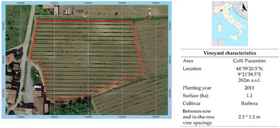
Figure 1.
Characteristics of the vineyard under study.
Vines were planted at a spacing of 2.5 m *× 1.2 m (between-row and in-the row distance, respectively) resulting in a potential vine density of 3333 vines/ha. Rows were established on an east-facing versant having a 15% longitudinal slope and trained to a single-cane vertically shoot positioned (VSP) Guyot trellis with a load of about 11 nodes/vine. The fruiting cane was raised 90 cm above the ground and surmounted by three catch wires for a canopy wall extending approximately 1.5 m above the main wire. The vineyard was managed according to the standard regional protocol for integrated viticulture; to maintain the most regular canopy shape hence minimizing the number of shoots hindering the alley space canopy were mechanically trimmed twice on 22 June and 2 August. Native cover crop was alternated to soil tillage every second mid-row, while the under-the-row vine strip (60 cm width) was managed with light tillage.
In 2016, a pool of 120 vines was randomly tagged immediately after budburst for subsequent measurements of vegetative growth, yield components and grape composition.
2.2. Remote Sensing
S2 is the multispectral imaging mission of the ESA Copernicus Earth Observation Program, based on a constellation of two identical satellites (S2A and S2B) in the same orbit at 786 km altitude. The multispectral instrument (MSI) onboard each satellite captures images in 13 spectral bands and ground resolution varies from 10 m for the visible, 20 m in the red-edge, narrow NIR and SWIR bands and 60 m for the atmospheric bands [20]. S2A acquisition of 11 July 2016 was chosen for comparison of spatial variability assessment with the other platforms. The European Space Agency’s (ESA) Sen2Cor algorithm was used to perform the atmospheric correction (Supplementary Figure S2).
Spot-6 was identified as the second satellite platform and the multispectral image of 15 July 2016 was bought (Supplementary Figure S2). Spot-6 acquires images at 6 m spatial resolution on four spectral bands specified as blue (450–520 nm), green (530–590 nm), red (625–695 nm), and near-infrared (NIR) (760–890 nm). A Pleiades image was acquired on 17 August 2016 (Supplementary Figure S2). The image consists of four bands at 2 m resolution: blue (430–550 nm), green (500–620 nm), red (590–710 nm), and NIR (740–940 nm). WorldView-3 provides images with multispectral bands in the VNIR region available at a resolution of 1.24 m, 8 bands in SWIR between 1195 and 2365 nm at a resolution of about 4 m and 12 bands for atmospheric correction as described in Table 1. A WorldView-3 image acquired on 16 July 2016 was used for platform comparison (Supplementary Figure S2).

Table 1.
Total leaf area, winter pruning weight per vine, yield/vine, cluster weight, total soluble solids, total anthocyanins on field-grown cv. Barbera grapevines (n = 120).
2.3. Proximal Sensing Platform
On 29 July an on-the-go acquisition at 3 Hz frequency with the MECS-VINE® proximity sensor was performed (Supplementary Figure S2). Using an algorithm named Canopyct, measurements allow obtaining an optical index, called Canopy Index (CI), represented by a pure number that varies from 0 to 1000 [19]. The Canopyct algorithm is based on the analysis of the images coming from the two RGB sensors, through which it calculates the color (Hue: H), the saturation (S), and the brightness (L) recording the coordinates of each pixel of the image. Then, the algorithm combines the RGB information with the components H, S, and L in order to return a result that can be expressed in a single dimension. Then, the clustering technique on the entire image is applied and the sensor derives a thematic map by assigning each pixel a distinguishable classification in: “Vegetation” and “Other”. The Canopy Index is finally calculated using the following formula:
CI = (N pixelVegetation)/(N pixelTotal) × 100
- N pixelVegetation: total number of pixels in the image classified as “vegetation”.
- N pixelTotal: total number of pixels in the image.
Every row was scanned twice on both sides and, in order to obtain an image in correspondence with each test plant, vines were geo-referenced and values were averaged to obtain a single CI value per plant at a spatial resolution of about 1.4 m, therefore quite close to the in-the-row vine spacing of the test vineyard (1.2 m).
2.4. Vegetative Growth, Yield, and Grape Composition
At cessation of shoot growth (approximately end of July), 120 vines next to those tagged, were selected and all main and lateral leaves from one shoot per plant were sampled; then each blade leaf area was determined through a leaf-area meter (Li-Cor Inc., Lincoln, NE, USA).
Soon after leaf abscission and before any immature wood portions (e.g., laterals) started to shed, total node number per vine was counted, separating main and lateral wood contributions. Combining average main and lateral single leaf area, cane number per vine and node counts allowed total leaf area per vine to be estimated. Thereafter, all vines were winter pruned to replenish the cane system and the total amount of removed one-year-old pruning weight was recorded.
At harvest, 19 September 2016, cluster number per vine and total grape weight were assessed. A 100-berry sample per vine was taken by removing berries from three basal clusters, taking care that both positions and exposure within the same cluster were well represented. A sub-sample of 50 berries was crushed and the resulting must was processed for total soluble solids (TSS) determined by a temperature-compensating refractometer (model RX-5000; ATAGO Ltd., Tokyo, Japan). The second set of 50-berry samples taken from the same clusters was used for measuring the total anthocyanins concentration after Iland [21]. The sample berries were homogenized at 20,000 rpm with an Ultra-Turrax (Rose Scientific Ltd., Edmonton, Canada) homogenizer for 1 min, then 2 g of the homogenate was transferred to a pre-tared centrifuge tube, enriched with 10 mL aqueous ethanol (50%, pH 5.0), capped and mixed periodically for 1 h before centrifugation at 959× g for 5 min. A portion of the extract (0.5 mL) was added to 10 mL 1 M HCL, mixed and let stand for 3 h; absorbance was then measured at 520 nm and 280 nm on a Kontron spectrophotometer (Tri-M Systems/Engineering, Toronto, Canada). Total anthocyanins concentration was given as mg per g of fresh berry mass.
2.5. Satellite Images Processing
Any S2, Spot-6, Pleiades and WorldView-3 image was subjected to atmospheric correction applied to the top of the canopy reflectance through the ENVI FLAASH algorithm and NDVI was then calculated according to Rouse et al. [22] as follows:
NDVI = (NIR − RED)/(NIR + RED)
Images were analyzed through the coefficient of variation (CV) that is calculated as the standard deviation to mean value ratio expressed as a percentage. GeoDa software [23] was used to perform the NDVI’s autocorrelation analysis through the univariate Moran’s statistic which can handle the spatial correlation among groups of paired plots at an increasing distance [24]. Moran index (MI) shows the degree of global autocorrelation among data in the area and varies from −1 to +1, where 0 reveals the absence of spatial autocorrelation (perfect randomness), −1 is perfect clustering of dissimilar values (perfect dispersion), whereas +1 indicates perfect clustering of similar values [25]. On each map, the univariate Moran statistic was considered in order to identify the degree of spatial autocorrelation detected by different ground resolution levels. The analysis was conducted using a queen contiguity approach with the first-order of neighbors for each acquisition [26].
2.6. Platform Comparison
Ordinary least square (OLS) regressions were considered to compare NDVI maps from different platforms and F-statistic was used to evaluate the significance of the regression model. Comparisons were performed using regression functions from GeoDa software and considering as covariates the vigor index values derived from the native resolution acquisition (10 m: Sentinel-2; 6 m: Spot-6; 2 m: Pleiades; 1.4 m: MECS-VINE®); while the values of the resampled images were imposed as the dependent variable. Models’ linearity was assessed through the Pearson correlation coefficient (r) [27]. In order to compare multispectral images with different spatial resolution through Moran’s statistic, higher resolution maps were resampled to the lower spatial resolution pixel dimension as it follows:
- Spot-6: 10 m ground resolution
- Pleiades: 6 m and 10 m ground resolution
- MECS-VINE®: 2 m, 6 m and 10 m ground resolution
- WorldView-3: 1.4 m, 2 m, 6 m and 10 m ground resolution
The Bivariate LISA (BILISA) was used to analyze the degree of spatial clustering and dispersion between features of a variable and another different variable in nearby locations [28].
For each image, queen spatial weight map was calculated as previously described and the bivariate Moran Index was used to perform the comparison between maps according to Matese et al. [26]. In each comparison the NDVI values from the native resolution were used as X values; as an example, in the comparison among 10 m resolution maps, Sentinel-2 values were used as X values, and NDVI from the other resampled maps were considered as Lag-X. Each Moran Index null hypothesis for statistical significance was then analyzed by the 999 random permutations and a Z-test. The significance test consists in the computation of a number of Monte-Carlo random permutations among locations. Critical Z-score values were considered using a 99% confidence level, significance was considered for results with a Z-score value below −2.576 and above +2.576.
Thereafter, the native images and resampled images at lower resolutions were used to calculate the 3-quantile vigor index (NDVI or CI) maps.
2.7. Intercomparison between Platforms and Ground Data
Ground data used were those assessed on the 120 geo-localized vines and regarded the following variables: total leaf area and total pruning weight per vine, yield per vine, total soluble solids (TSS), and anthocyanins concentration. OLS was run using GeoDa software as previously described. Variables were analyzed in separate models using vigor index (NDVI or CI) values and agronomic data as covariates and dependent variables, respectively. F-statistic was used to evaluate the significance of the regression model. Bivariate Moran index was calculated using two different approaches, hereafter named Moran 1 and Moran 2.
Moran 1 (M1). It consisted of the comparison between NDVI values as X and ground data al Lag-X. Agronomical values were then associated to each native NDVI map; when pixels size warranted enough spatial ground resolution, a univocal NDVI value was associated with each vine; conversely, ground data were averaged when multiple plants were comprised into the same pixel. Then, new maps were built with the same resolution as the natives but considering only those pixels that were coupled to the ground values. Spatial weight matrices were managed using bandwidths of 14.1 m, 12.2 m, 8.2 m, and 8.6 m for S2, Spot-6, Pleiades, MECS-VINE® and WorldView-3, respectively, and 999 random permutations and Z-score test were performed as previously described.
Moran 2 (M2). Ordinary kriging was applied to agronomic data and five maps were created at 10 m, 6 m, 2 m, 1.4 m, and 1.24 m spatial resolution and subsequently coupled with the corresponding native NDVI grid. Moran 2 was then calculated using ground data as X values and NDVI as Lag X. Spatial weight matrices were calculated using queen contiguity approach with the first-order of neighbors, and 999 random permutations and Z-score test were performed as mentioned above.
3. Results
3.1. Vigor Variability and Vine Performance
The 2016 season was quite representative of the average climate trend of the area with growing degree days (GDD) calculated from 1 April to 30 September setting at 1944 GDD [29] whereas precipitation summed up to 758 mm over the same time span. Total pruning weight per vine largely differed among vines ranging between 0.27 kg and 2.09 kg and showed the highest CV of 33.9% (Table 1). Another vine capacity variable, total leaf area, had slightly less variation among vines with a CV of 24.1%. Although mean yield was 5.63 kg/vine, the maximum value was about ten-fold higher than the minimum (i.e., 11.8 kg vs. 1.5 kg, respectively) and the calculated CV was 24.1%.
In terms of grape composition at harvest, the most sensitive to variations in vigor was total anthocyanins concentration, varying from 0.12 to 2.53 mg/g with a CV of 27.3%. Conversely, TSS showed a moderate CV (9.7%), although minimum and maximum differed by 10 °Brix (17.5 and 27.8 °Brix, respectively). With respect to the univariate Moran index calculated for each variable, analyses showed that total pruning weight/vine and total leaf area/vine had a similar index (0.32 and 0.34). Quality parameters settled around 0.22, while production/vine had the highest Moran index value of 0.41 (Table 1).
3.2. Spatial Variability Assessment with Different Sensing Platforms
Table 2 reports the basic statistics at native resolution for the NDVI index values for each satellite platform, whereas statistics are referred to as Canopy Index (CI) values in the case of MECS-VINE®. The highest mean NDVI (0.711) was calculated for WorldView-3 acquired images followed by S2 and Spot-6 (0.668 and 0.654, respectively). WorldView-3 had the highest CV (12.6%), while MECS-VINE® the lowest (7.6%). Despite the highest mean NDVI, WorldView-3 also recorded the lowest minimum (0.107). Regarding the Moran Univariate index calculated on NDVI or CI bases, all platforms showed positive values and the value of the index gradually rose with increasing spatial resolution, peaking at 0.903 in MECS-VINE®.
Table 2.
Basic statistics at native resolution.
Figure 2 shows the cluster maps derived from the calculated univariate Moran index: the red and dark blue pixels indicate the matching correspondences (H-H and L-L), while lighter colors indicate the discordant comparisons (L-H and H-L). Usually, non-matching correspondences are found mostly in the transition areas between high and low values, except for in the S2 map, where these matches were also present on border pixels.
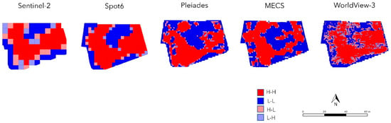
Figure 2.
LISA cluster map of Moran univariate Index based on vigor index value (NDVI or CI). The analysis was conducted using a queen contiguity approach with the first-order of neighbors for each acquisition. Different colors correspond to four types of local spatial autocorrelation (red = High-High; dark blue = Low-Low; light red = High-Low; light blue = Low-High).
Figure 3A–E shows the vigor maps calculated from NDVI and CI according to three classes defined using tertiles. The same figure also shows vigor maps for images resulting from resampling at lower resolution. The spatial distribution of quantiles in the different maps always distinctly showed two areas, namely a high vigor area in the Southernmost part of the vineyard, and a low vigor area in the Northernmost sector (Figure 3A–E). Supplementary Table S1 shows the extreme NDVI and CI values of each vigor class. In all maps, low vigor interval was always the widest class corresponding to 0.275 in S2, 0.212 Spot-6, 0.247 Pleiades, 207 MECS-VINE®, and 0.522 in Wv3. The highest difference between minimum and maximum of a single class is for Q1 of WV-3 (0.59). In all platforms, the distribution of tertile class shows the largest change when resampling is performed from 6 m to 10 m.
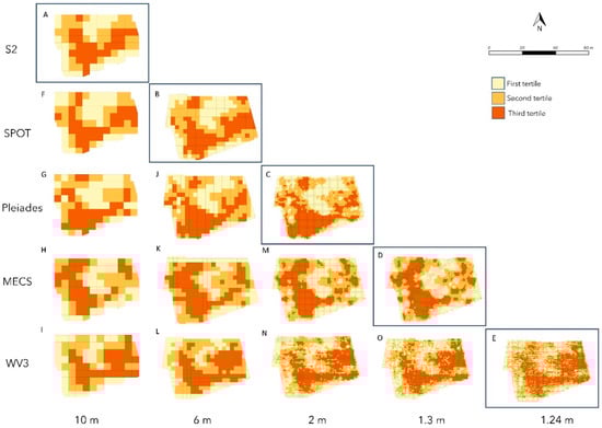
Figure 3.
Map of NDVI index (S2, Spot-6, Pleiades, and WorldView-3) or CI (MECS-VINE®). Levels were partitioned by tertiles. Squared boxes represent vigor maps processed at the native resolution of each platform. Higher resolution maps were resampled to the lower spatial resolution pixel dimension as it follows: Spot-6, 10 m ground resolution; Pleiades, 6 m and 10 m ground resolution; MECS-VINE®, 2 m, 6 m, and 10 m ground resolution; WorldView-3, 1.4 m, 2 m, 6 m, and 10 m ground resolution.
Table 3 reports R2 coefficients for ordinary least squares (OLR) regressions between vigor indices at native resolution and those derived from other platforms when resampled at the same spatial resolution. For any single linear regression between platforms, R2 values from OLR analysis were highly significant (p < 0.01) albeit the degree of correlation varied from low (r = 0.18) for S2 NDVI vs. the re-sampled Pleiades to high (r = 0.68) calculated for Spot-6 NDVI vs. re-sampled WorldView-3.
Table 3.
Coefficients of determination (R2) of quantitative comparison between different platforms using OLS. The images were resampled as follows: Spot-6, 10 m ground resolution; Pleiades, 6 m and 10 m ground resolution; MECS-VINE®, 2 m, 6 m and 10 m ground resolution; WorldView-3, 1.4 m, 2 m, 6 m and 10 m ground resolution. Comparisons were performed by considering as the independent variable the vigor index value (NDVI or CI) derived from the native resolution acquisition (10 m: Sentinel-2; 6 m: Spot-6; 2 m: Pleiades; 1.4 m: MECS-VINE®), while the values of the resampled images were assumed as the dependent variable.
Moran index (MI) calculated between the same variable combinations was always significant and a positive spatial autocorrelation could be ascertained in all cases (Table 4); the best clustering of similar values (Moran index of 0.51) was seen for Spot-6 vs. WorldView-3, whereas the highest dispersion (Moran index = 0.26) was observed in the S2 vs. MECS-VINE® comparison.
Table 4.
Quantitative comparison between different platforms using bivariate Moran Index. The images were resampled as it follows: Spot-6, 10 m ground resolution; Pleiades, 6 m and 10 m ground resolution; MECS-VINE®, 2 m, 6 m, and 10 m ground resolution; WorldView-3, 1.4 m, 2 m, 6 m, and 10 m ground resolution. Comparisons were performed by considering as X the vigor index value derived from the native resolution acquisition (10 m: Sentinel-2; 6 m: Spot-6; 2 m: Pleiades; 1.4 m: MECS-VINE®), while the values of the resampled images were assumed as LagX.
Figure 4 reports graphical BILISA comparisons across cluster maps. Ratios-matching (H-H and L-L) was found mainly in the two areas of high and low vigor located in the southernmost and northernmost part of the vineyard, respectively. Non-matching pixels (H-L and L-H) were present especially in the areas of transitions between these two areas. The cluster map resulting from the comparison between Spot-6 and Pleiades had the highest number of matching pixels among the maps under evaluation, as 90% of the pixels belong to the categories H-H or L-L.
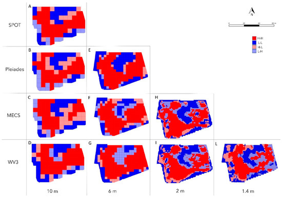
Figure 4.
BILISA cluster map based on the Moran bivariate Index. The images were resampled as it follows: Spot-6, 10 m ground resolution; Pleiades, 6 m and 10 m ground resolution; MECS-VINE®, 2 m, 6 m, and 10 m ground resolution; WorldView-3, 1.4 m, 2 m, 6 m, and 10 m ground resolution. Comparisons were performed by considering as the independent variable the vigor index value (NDVI or CI) derived from the native resolution acquisition (10 m: Sentinel-2; 6 m: Spot-6; 2 m: Pleiades; 1.4 m: MECS-VINE®), while the values of the resampled images were assumed as the dependent variable. The analysis was conducted using a queen contiguity approach with the first-order of neighbors for each acquisition. Different colors correspond to four types of local spatial autocorrelation (red = High-High; dark blue = Low-Low; light red = High-Low; light blue = Low-High).
Table 5 shows R2 coefficients for simple linear regressions made by plotting the NDVI values and the respective values of agronomic variables. The linear model was highly significant for almost any variable except for TSS which was much less responsive. Across the different platforms, the highest R2 was shown by NDVI vs. pruning weight and yield per vine parameters. Interestingly the closest relationship was found in S2-derived images for the combination of NDVI vs. total anthocyanins concentration (R2 = 0.34).
Table 5.
Coefficients of determination (R2) of quantitative comparison between different platforms and ground data using OLS regression coefficient.
M1 values, calculated using NDVI values as X and agronomic data as lag X, show the highest coefficients for Pleiades, Spot-6, and MECS-VINE® (Table 6). Most robust comparisons were found for total pruning weight per vine (0.53 for Pleiades, 0.45 for Spot-6, and 0.50 for MECS-VINE®). As with OLS, S2 and WorldView-3 had the low index values (0.27 and 0.32 on average, respectively). When considering the five platforms, total leaf area per vine had a slightly lower spatial autocorrelation index as compared to total pruning weight (0.36 vs. 0.44). M1 calculated for TSS determined at harvest exhibited a negative sign although in one case (WorldView-3) significance was not reached. A more consistent trend was shown for M1 calculated over total anthocyanins concentration with values varying between 0.31 (S2) and 0.47 (Pleiades).
Table 6.
Moran 1 (M1), quantitative comparison between different platforms and ground data using bivariate Moran Index. M1 NDVI values as X and ground data al Lag-X.
M2, calculated using agronomic data as x and NDVI as lagX shows a similar trend to that already seen in Moran1 (Table 7). However, a common feature was that, regardless of the sign of the spatial autocorrelation, S2 scored decidedly lower M2 values than any other platform. Similarly, to M1, Pleiades achieved the highest mean M2 with a peak of 0.58 for total pruning weight per vine.
Table 7.
Moran 2(M2), quantitative comparison between different platforms and ground data using bivariate Moran Index. M2 was calculated using ground data as X values and NDVI as LagX.
4. Discussion
Data shown in Table 1 for agronomic variables allow the estimation of the degree of intra-plot variability that, despite the small vineyard size, was quite large. Interestingly, CV calculated for winter pruning weight was 33.9% representing the highest variability among the considered parameters. This is in line with Gatti et al. [8] who reported that pruning weight was a very good descriptor of vigor and, in that scenario, ranged from 0.92 to 1.2 kg/vine in low and high vigor zones, respectively. Likewise, a close correlation between vine pruning weight and NDVI derived from S2 acquisitions was found in the cultivar Verdejo when working on three hedgerow-trained vineyards belonging to the Appellation of Origin Rueda [30]. Similar variability was assessed for the other indicator of vine capacity, total leaf area, which varied between 1.73 m2 and 6.77 m2 per vine. This wide range identifies very sparse canopies with several gaps in low vigor, and thicker canopies in high vigor exceeding the limit of about 4 m2/m of row beyond which canopy density is considered to be suitable for leaf removal [31].
Similarly to pruning weight CV calculated for yield/vine was higher than 30% revealing a significant yield variation within the 1.5 ha block. This performance is analogous to what is already described by Gatti et al. [32] in an older Barbera vineyard from the same region highlighting temporal stability of patterns of intra-vineyard variations.
Despite varying between 17.5 and 27.5 °Brix, TSS was the least variable (CV = 9.74%). While this result finds confirmation in previous work where intra-vineyard spatial and temporal variability of sugar concentration have shown, when compared to growth or yield performance, less dependence vs. NDVI-based vigor levels [33], there is also physiological ground for that. Albeit vigor greatly varies among different vineyard parcels, it should be kept in mind that the level of sugar concentration accumulated into the grape berry is primarily a function of the leaf area-to-yield ratio [34] and that non-limited sugar accumulation is reached anytime such a ratio sets above 1 m2/kg of fruit. This means that, not necessarily, higher vigor manifested as increased leaf area and yield will correspond to lower TSS as long as enough leaf area is present on the vine to ripen the fruits. Average LA/Y calculated from Table 1 data is 0.67 m2/kg that, despite being indeed sub-optimal, did not prevent vines to reach 22.8 Brix and 1.28 mg/kg total anthocyanins, a compositional pattern suitable for high-quality red winemaking. Notably, intra-vineyard variability assessed for total anthocyanins was larger than that for TSS, although color formation should also respond to leaf-to-fruit ratio. Such differential behavior of TSS and anthocyanins concentration at responding to spatial Intra-vineyard variability should likely consider that color accumulation is much more affected than TSS from local light and temperature microclimate insisting on the fruiting area. Thus, it is very likely that low vigor areas lead to better cluster light availability, hence better color, whereas increasing shade cast on fruiting zones in more vigorous spots is more detrimental for anthocyanins accumulation in the berry [8].
A Moran index value of 0 indicates that there is no spatial auto-correlation (i.e., perfect randomness) between a variable at one point and the same variable measured at neighboring points [26]; in our work, yield per vine and weight of pruning wood showed the highest Moran index among the measured parameters indicating that they held strong spatial autocorrelation, which means that values changed more gradually across adjacent pixels. There is a good consensus that intra-vineyard spatial variability is quite stable over time [14,35] and is mostly related to the patchiness in the soil’s physico-chemical features affecting the water-holding capacity, water infiltration rate, nutrient availability and uptake, that usually manifest on a scale of several meters. This would explain why, along a single row, very rarely vigor changes abruptly from vine to vine, rather following a larger spatial pattern. As confirmed by lower MI in Table 1, the same concept does not necessarily apply to quality variables such as TSS and color whose spatial variability can be more easily affected by management strategies such as summer pruning (for instance a high vigor vine subjected to basal leaf removal is shifted, as per TSS and color, toward a low vigor behavior).
The NDVI value distribution indicates WorldView-3 as the platform with the largest CV (Table 2). Looking at the minimum and maximum values and considering that the ground resolution was 1.24 m, it is very likely that World-View-3 image acquisition also included pure soil pixels having quite low NDVI values. A simple geometrical calculation can be made to highlight that at the given between-row vine spacing of 2.5 m and assuming average canopy thickness of about 60 cm, zenithal soil view is restricted to 1.9 m which can easily accommodate “pure soil” pixels in WorldView-3 whereas all remaining satellite platforms—having resolutions >2 m—are bound to a mixel view including a different proportion of vineyard row. As also highlighted in a study conducted by Ding et al. [36], where the variability of soil NDVI was investigated, the range within which NDVI describes the bare soil settles between 0.07 and 0.22. Accordingly, the lowest value of 0.107 based on our WorldView-3 acquisition may describe the soil status that was repeatedly tilled every second row during the season. Moreover, the higher the ground resolution the higher the minimum NDVI value revealing mixed conditions combining different proportions of grapevine canopies as well as of grassed vs. tilled soil.
From Table 2, the Moran index steadily increased in satellite platform according to increased spatial resolution (S2 < Spot-6 < Pleiades), to confirm previous work by Qi and Wu [37], who proposed a log-linear function relating the MI coefficients to resolution levels. However, expectations for having the highest MI scored in WorldView-3 were disappointing and, once again, the main cause seems to be the possible abrupt switch from pure soil pixel NDVI to mixel NDVI.
It is also interesting to observe that the highest MI value reached by one of satellite platforms (Pleiades, 0.822) was outscored by the MECS-VINE® platform (0.903) (Table 2). Between these platforms, the final pixel resolution diverges by 0.6 m (2 m in Pleiades versus 1.4 m in MECS-VINE®) and such difference can partly explain higher MI for MECS-VINE®. However, it must also be reminded that MECS-VINE® is a device that detects the level of vigor by taking proximal sensing readings and returning a value called “Canopy Index”, varying between 0 and 1000, that can be considered as an alternative method to the NDVI approach for assessing grapevine vigor in hedgerow-trained vineyards. As described in Gatti et al. [19], the sensor is mounted in front of the tractor and the on-the-go field of view directly hits canopy sectors therefore restituting pure-canopy pixels with no interference from grass or bare soil pixels. Having a ground resolution of 2 m, Pleiades invariably catches soil-canopy boundaries, and this would decrease the degree of spatial autocorrelation. This pattern is also visualized and confirmed by the cluster maps reported in Figure 2 as pixels with discordant correlations (L-H and H-L) decreased from 8% in Pleiades to 4% in MECS-VINE®. Generally, the vineyard was highly variable, and this can also be evidenced by the univariate Moran index calculated from S2 data, which was 0.325. A study conducted by Pastonchi et al., [38], reported Moran Univariate values calculated on the NDVI of S2 averaging 0.67. Unfortunately, the same authors while stating that their ground truthing included vigor parameters such as pruning weight and yield, did not provide any quantitative estimate or variation intervals for such parameters and so the extent of spatial intra-vineyard variability remained unresolved.
A border-pixel effect was also clear when analyzing the vigor maps showing NDVI distribution over the three tertiles (Figure 2). S2 and Spot-6 show areas of low vigor that are more concentrated along the vineyard boundaries. Moreover, a vertical comparison of all maps calculated at 10 m resampling (Figure 2A,F–I) shows that, out of 33 edge pixels, 21 pixels (i.e., 64%) fall into the first quantile when S2 images are considered. In the other satellite maps, where the pixel values come from the resampling at higher spatial resolution, the number of border pixels in the first tertile strongly decreased (~−16%). The comparison between 10 m maps showed that S2′s major border effect poorly represented the true variability pattern of the vineyard by identifying areas of potentially low vigor near the perimeter zones.
A quite interesting effect can be appreciated when analyzing the vigor map processed from the WorldView-3 image at 1.24 m (Figure 3E). The color pattern allows the identification of rather consistent strips essentially following the mid-row and under the row corridors, a further confirmation that NDVI derived from World-View-3 image acquisition provides a sharper separation between pure soil pixel and mixels. Resampling images at lower resolutions, this soil effect decreases as pure soil pixels are increasingly replaced with mixels (Supplementary Table S1). In each platform, even resampling at lower spatial resolutions, the range of vigor index classes calculated on the tertiles remains rather homogeneous. However, when resampling is done from 6 m to 10 m, the distribution of tertiles class range undergoes a significant change in all platforms. This suggests that at 10 m there is a large change in the descriptive quality of intraplot variability due to oversized pixels, despite the fact that the maps in panels F-G-H-I were made with data resampled from higher spatial resolutions.
Platform comparisons computed via simple regressions of NDVI and CI values derived from native resolution acquisition (x) vs. NDVI and CI derived from resampled images (y) values highlight that not necessarily an increase in resolution leads to an increase in R2 (Table 3). It is also relevant that the regressions with the lowest coefficient of determination are those that emerged from S2. This can also be explained considering results from Sozzi et al. [17] where a comparison was made between NDVI values calculated by S2 and those acquired by a UAV confirming that the R2 of the regressions increased by 8% once border pixels were excluded. This type of trend is even clearer once the comparison is made on a geo-statistical basis (Table 4). In fact, the bivariate Moran index of S2 is markedly lower than that of the other platforms. Analyzing Figure 4, where BILISA cluster maps were created by comparing the pixels of the native image with the resampled images, it is noticeable that, at 10 m, the comparisons, in which there was an L-H or H-L match, were located not only at the vineyard boundaries but also in the central zone (Figure 4A–D). For this reason, it is possible to conclude that the low coefficient that emerged from the comparisons at 10 m can be attributed to two effects: (i) the border pixels that under low resolutions are more heavily impacted by the interference of the soil around the vineyard and (ii) the poorer ability of S2 to detect a transition from high and low vigor areas and vice versa.
In both the OLS and Moran analyses, TSS is the parameter that has the lowest indices (Table 5, Table 6 and Table 7). This was already observed in Table 1 and a physiological hypothesis was given to justify the quite poor auto-correlation of this variable. The same behavior was confirmed by a study conducted in Tuscany, where again TSS always had the lowest degree of correlation with NDVI values [38]. Spot-6 shows on average the highest coefficient of determination among platforms and in particular seems to be a good predictor of pruning weight, yield, and anthocyanin content. This is in line with what was shown by Gatti et al. [32] in a study in which the NDVI index calculated at 5 m was used to make comparisons with agronomic data. Also, in that case, the vigor index closely correlated with vegetative, yield, and grape composition parameters.
To better assess the reliability of platforms at describing spatial variability of agronomic variables, it is necessary to focus the analysis on the two indices that consider the degree of spatial autocorrelation [26]. Moran’s index1 was calculated using only the pixels in which the ground-truthed vines were located, and the matrix of weights was built with the minimum possible distance (Table 6). Conversely, M2 was calculated using agronomic values as the independent variable and a first-degree queen matrix to compare the neighborhood of pixels (Table 7). Regardless of the type of Moran index used, TSS confirms having the lowest degree of spatial autocorrelation and the negative sign suggests a moderate degree of dispersion. Reading it another way, in M1, having NDVI as X variable and lag X the ground-truthed agronomic variable, similar NDVI might correspond to largely different TSS levels. In M2, the overall scenario is similar although Z-scores indicated that a randomness status was ascertained for the Sentinel-2 images. Moreover, in Table 6 and Table 7 yield per vine and pruning weight per vine were those with the highest Bi-variate Moran Index among the investigated comparisons (total pruning weight/vine: M1 = 0.44, M2 = 0.47; yield/vine: M1 = 0.39, M2 = 0.40, averaged across platforms). According to M1 and M2, a robust inverse spatial autocorrelation was found for the concentration of total anthocyanins whose degree of spatial autocorrelation averaged −0.38 and −0.42, respectively. From an agronomic point of view, it is expected that lower NDVI, hence reduced vigor, may promote synthesis and color accumulation due to better illumination.
Another variable showing poor spatial correlation, especially when referred to the S2 platform, is total leaf area per vine. Such a pattern links to results reported by Velez et al. [39] investigating the effect of missing vines on total leaf area by calculating NDVI from S2 images. It was demonstrated that the decrease in total leaf area within any pixel area was more than proportional to the decrease in NDVI. In particular, when the leaf area was reduced by 20%, the decrease in NDVI corresponded to about 6–7%. Although in our Barbera field there were no missing vines, the lowest M1 and M2 scored by S2 for total leaf area per vine indicate that low resolution can be a bias. Conversely, when the total leaf area is analyzed by any other platforms, both Moran indices increase to a maximum of 0.44 to confirm that narrowing the space around the ground-truthed test vine might better show the actual degree of autocorrelation.
In the case of WorldView-3, the satellite platform boasting higher ground resolution (1.24 m), the two Moran indices did not exceed 0.31 for data pooled over all agronomic variables. While this clearly relates back to previously discussed pixel composition, it also suggests that the WorldView-3 image might need additional pixel extraction and selection procedures, as also done by Solano et al. [40]. In this case, the hyperspherical color space (HCS) resolution merge pan-sharpening algorithm [41] was applied to the multispectral image at 1.24 m in order to merge it with the pan band (0.31 m), and an extraction of olive tree canopies was subsequently performed, thus cancelling out the soil effect.
The platform with the most consistent comparisons across all variables was Pleiades scoring the highest average indices among the compared platforms (M1: 0.44; M2: 0.51), followed by MECS-VINE® (M1: 0.38 average; M2: 0.44 average). In both cases, the level of effectiveness in vineyard analysis was quite accurate. Not only they obtained optimal results as indicators of the vegetative status, but they also showed that NDVI calculated at about 2 m spatial resolution, could be a good indicator also of the qualitative parameters of the must, such as anthocyanins concentration, both for remote and proximal sensing. These results suggest that although the ground resolution of Pleiades inevitably creates mixed soil-canopy pixels, they effectively characterize vineyard variability. This may be due to the presence of native grassing every second mid-row which may have mitigated the negative effect of soil in mixels.
5. Conclusions
The aim of the study was to investigate the acquisition accuracy of satellite and proximal platforms having different spatial resolution. In the case of a vertically shoot positioned vineyard having alternate rows with native grass and tilled soil, the platforms that performed better were Pleiades and MECS-VINE®. The good descriptive effectiveness of the latter was ensured by the acquisition mode of proximal sensing that allowed to overcome the limit of border pixels, often not very descriptive in the case of satellite platforms and avoided the presence of mixed vegetation-soil pixels (mixels). This seems to be the most suitable solution especially in the case of studying vineyards with irregular margins, where the influence of the border pixel becomes predominant. At the same time, under the experimental conditions, satellite imagery at 2 m ground resolution (Pleiades) also ensured a quite robust descriptive effectiveness despite soil pixels were not excluded and actually averaged in the so-called mixels. Conversely, when spatial resolution reaches high levels, yet not sufficient to apply inter-row filtering, as in the case of WorldView-3, results are less satisfactory. Despite the fact that S2 represents a tool with great potential since it is a free resource with a high-resolution time, this platform did not achieve an accurate description of intra-plot variability, especially in margin and intermediate vigor zones. As a matter of fact, the noticeable border effect seems to be very limiting especially for vineyards of small size or having a very irregular shape, typical of Italian viticulture. Moreover, in contrast to what it has been reported in other studies where Sentinel-2 was used to study the field crops forming a continuous land cover (e.g., corn, wheat, or even forest systems), in the case of the vineyard discontinuous land cover coupled with the pixel size decreased the effectiveness of this tool. In the case of low-to-medium ground resolutions, 6 m of ground resolution certainly seems to be the optimal solution.
Supplementary Materials
The following are available online at https://www.mdpi.com/article/10.3390/rs13112056/s1. Table S1: Class ranks of vigor maps calculated from NDVI or CI. Levels were partitioned by tertiles, bold: maps calculated at native resolution. Higher resolution maps were resampled to the lower spatial resolution pixel dimension as it follows: Spot6, 10 m ground resolution; Pleiades, 6 m and 10 m ground resolution; MECS-VINE®, 2 m, 6 m and 10 m ground resolution; WorldView-3, 1.4 m, 2 m, 6 m and 10 m ground resolution.
Author Contributions
Conceptualization, C.S., S.P., S.F.D.G., A.M., and M.G.; methodology, C.S., S.F.D.G., and A.M.; software, C.S., S.F.D.G., and A.M.; validation, C.S., S.P., and M.G.; formal analysis, C.S.; investigation, C.S.; resources, S.P.; data curation, C.S., S.F.D.G., and A.M.; writing—original draft preparation, C.S. and S.P.; writing—review and editing, S.F.D.G., S.P., and M.G.; visualization, C.S.; supervision, S.P.; project administration, C.S.; funding acquisition, S.P. All authors have read and agreed to the published version of the manuscript.
Funding
This research was funded by Emilia-Romagna Region within Nutrivigna project under the grant POR-FESR 2014-2020.
Institutional Review Board Statement
Not applicable.
Informed Consent Statement
Not applicable.
Data Availability Statement
The raw data supporting the conclusions of this article will be made available by the authors, without undue reservation, to any qualified researcher.
Acknowledgments
The authors acknowledge Paolo Malvicini for hosting the trial, Massimo Vincini, Ekaterina Kleshcheva and Alessandra Garavani for technical support, Paolo Dosso and Bonfiglio Platé for technical assistance during proximal sensing and CI mapping.
Conflicts of Interest
The authors declare no conflict of interest.
References
- Zhang, N.; Wang, M.; Wang, N. Precision agriculture—A worldwide overview. Comput. Electron. Agric. 2002, 36, 113–132. [Google Scholar] [CrossRef]
- Wolfert, S.; Ge, L.; Verdouw, C.; Bogaardt, M.J. Big Data in Smart Farming—A review. Agric. Syst. 2017, 153, 69–80. [Google Scholar] [CrossRef]
- Pierpaoli, E.; Carli, G.; Pignatti, E.; Canavari, M. Drivers of Precision Agriculture Technologies Adoption: A Literature Review. Procedia Technol. 2013, 8, 61–69. [Google Scholar] [CrossRef]
- Rudd, J.D.; Roberson, G.T.; Classen, J.J. Application of satellite, unmanned aircraft system, and ground-based sensor data for precision agriculture: A review. In Proceedings of the 2017 ASABE Annual International Meeting, Spokane, WA, USA, 16–19 July 2017; pp. 1–8. [Google Scholar] [CrossRef]
- Maestrini, B.; Basso, B. Predicting spatial patterns of within-field crop yield variability. F. Crop. Res. 2018, 219, 106–112. [Google Scholar] [CrossRef]
- Batchelor, W.D.; Basso, B.; Paz, J.O. Examples of strategies to analyze spatial and temporal yield variability using crop models. Eur. J. Agron. 2002, 18, 141–158. [Google Scholar] [CrossRef]
- Bramley, R.G.V. Precision Viticulture: Managing vineyard variability for improved quality outcomes. In Managing Wine Quality: Viticulture and Wine Quality; Elsevier Inc.: North York, ON, Canada, 2010; pp. 445–480. ISBN 9781845694845. [Google Scholar]
- Gatti, M.; Schippa, M.; Garavani, A.; Squeri, C.; Frioni, T.; Dosso, P.; Poni, S. High potential of variable rate fertilization combined with a controlled released nitrogen form at affecting cv. Barbera vines behavior. Eur. J. Agron. 2020, 112. [Google Scholar] [CrossRef]
- Maes, W.H.; Steppe, K. Perspectives for Remote Sensing with Unmanned Aerial Vehicles in Precision Agriculture. Trends Plant Sci. 2019, 24, 152–164. [Google Scholar] [CrossRef]
- Matese, A.; Toscano, P.; Di Gennaro, S.F.; Genesio, L.; Vaccari, F.P.; Primicerio, J.; Belli, C.; Zaldei, A.; Bianconi, R.; Gioli, B. Intercomparison of UAV, aircraft and satellite remote sensing platforms for precision viticulture. Remote Sens. 2015, 7, 2971–2990. [Google Scholar] [CrossRef]
- Santesteban, L.G. Precision viticulture and advanced analytics. A short review. Food Chem. 2019, 279, 58–62. [Google Scholar] [CrossRef]
- Rossi, R.; Pollice, A.; Diago, M.P.; Oliveira, M.; Millan, B.; Bitella, G.; Amato, M.; Tardaguila, J. Using an automatic resistivity profiler soil sensor on-the-go in precision viticulture. Sensors 2013, 13, 1121–1136. [Google Scholar] [CrossRef]
- Arnó, J.; Rosell, J.R.; Blanco, R.; Ramos, M.C.; Martínez-Casasnovas, J.A. Spatial variability in grape yield and quality influenced by soil and crop nutrition characteristics. Precis. Agric. 2012, 13, 393–410. [Google Scholar] [CrossRef]
- Kazmierski, M.; Glemas, P.; Rousseau, J.; Tisseyre, B. Temporal stability of within-field patterns of ndvi in non irrigated mediterranean vineyards. J. Int. des Sci. la Vigne du Vin 2011, 45, 61–73. [Google Scholar] [CrossRef]
- Kazakou, E.; Violle, C.; Roumet, C.; Navas, M.L.; Vile, D.; Kattge, J.; Garnier, E. Are trait-based species rankings consistent across data sets and spatial scales? J. Veg. Sci. 2014, 25, 235–247. [Google Scholar] [CrossRef]
- Di Gennaro, S.F.; Dainelli, R.; Palliotti, A.; Toscano, P.; Matese, A. Sentinel-2 validation for spatial variability assessment in overhead trellis system viticulture versus UAV and agronomic data. Remote Sens. 2019, 11, 2573. [Google Scholar] [CrossRef]
- Sozzi, M.; Kayad, A.; Marinello, F.; Taylor, J.A.; Tisseyre, B. Comparing vineyard imagery acquired from sentinel-2 and unmanned aerial vehicle (UAV) platform. Oeno One 2020, 54, 189–197. [Google Scholar] [CrossRef]
- Giorgia Bucci; Deborah Bentivoglio; Adele Finco Factors affecting ICT adoption in Agriculture: A case study in Italy. Access Success 2019, 20, 122–129.
- Gatti, M.; Dosso, P.; Maurino, M.; Merli, M.C.; Bernizzoni, F.; Pirez, F.J.; Platè, B.; Bertuzzi, G.C.; Poni, S. MECS-VINE®: A new proximal sensor for segmented mapping of vigor and yield parameters on vineyard rows. Sensors 2016, 16, 2009. [Google Scholar] [CrossRef]
- Claverie, M.; Ju, J.; Masek, J.G.; Dungan, J.L.; Vermote, E.F.; Roger, J.C.; Skakun, S.V.; Justice, C. The Harmonized Landsat and Sentinel-2 surface reflectance data set. Remote Sens. Environ. 2018, 219, 145–161. [Google Scholar] [CrossRef]
- Iland, P.G.; Cynkar, W.; Francis, I.L.; Williams, P.J.; Coombe, B.C. Optimisation of methods for the determination of total and red-free glycosyl glucose in black grape berries of Vitis vinifera. Aust. J. Grape Wine Res. 1996, 2, 171–178. [Google Scholar] [CrossRef]
- Rouse, J.W.; Haas, R.H.; Schell, J.A.; Deering, D.W.; Harlan, J.C. Monitoring the Vernal Advancement of Retrogradation of Natural Vegetation; NASA/GSFC, Type III, Final Report; NASA: Greenbelt, ML, USA, 1974; p. 371.
- Anselin, L.; Syabri, I.; Kho, Y. GeoDa: An Introduction to Spatial Data Analysis. Geogr. Anal. 2006, 38, 5–22. [Google Scholar] [CrossRef]
- Chen, Y. New Approaches for Calculating Moran’s Index of Spatial Autocorrelation. PLoS ONE 2013, 8. [Google Scholar] [CrossRef] [PubMed]
- Getis, A.; Ord, J.K. The Analysis of Spatial Association by Use of Distance Statistics. Geogr. Anal. 1992, 24, 189–206. [Google Scholar] [CrossRef]
- Matese, A.; Di Gennaro, S.F.; Santesteban, L.G. Methods to compare the spatial variability of UAV-based spectral and geometric information with ground autocorrelated data. A case of study for precision viticulture. Comput. Electron. Agric. 2019, 162, 931–940. [Google Scholar] [CrossRef]
- Akaike, H. A New Look at the Statistical Model Identification. IEEE Trans. Automat. Contr. 1974, 19, 716–723. [Google Scholar] [CrossRef]
- Anselin, L.; Rey, S.J. Modern Spatial Econometrics in Practice: A Guide to GeoDa, GeoDaSpace and PySAL; GeoDa Press: Chicago, IL, USA, 2014. [Google Scholar]
- Winkler, A.J. General Viticulture; University of California Press: Berkeley, CA, USA, 1965. [Google Scholar]
- Vélez, S.; Rubio, J.A.; Andrés, M.I.; Barajas, E. Agronomic classification between vineyards (‘Verdejo’) using NDVI and Sentinel-2 and evaluation of their wines. Vitis J. Grapevine Res. 2019, 58, 33–38. [Google Scholar] [CrossRef]
- Kliewer, W.M.; Dokoozlian, N.K. Leaf area/crop weight ratios of grapevines: Influence on fruit composition and wine quality. Am. J. Enol. Vitic. 2005, 56, 170–181. [Google Scholar]
- Gatti, M.; Garavani, A.; Vercesi, A.; Poni, S. Ground-truthing of remotely sensed within-field variability in a cv. Barbera plot for improving vineyard management. Aust. J. Grape Wine Res. 2017, 23, 399–408. [Google Scholar] [CrossRef]
- Trought, M.C.T.; Bramley, R.G.V. Vineyard variability in Marlborough, New Zealand: Characterising spatial and temporal changes in fruit composition and juice quality in the vineyard. Aust. J. Grape Wine Res. 2011, 17, 72–78. [Google Scholar] [CrossRef]
- Poni, S.; Gatti, M.; Palliotti, A.; Dai, Z.; Duchêne, E.; Truong, T.T.; Ferrara, G.; Matarrese, A.M.S.; Gallotta, A.; Bellincontro, A.; et al. Grapevine quality: A multiple choice issue. Sci. Hortic. 2018, 234, 445–462. [Google Scholar] [CrossRef]
- Taylor, J.A.; Bates, T.R. A discussion on the significance associated with Pearson’s correlation in precision agriculture studies. Precis. Agric. 2013, 14, 558–564. [Google Scholar] [CrossRef]
- Ding, Y.; Zheng, X.; Zhao, K.; Xin, X.; Liu, H. Quantifying the impact of NDVIsoil determination methods and NDVIsoil variability on the estimation of fractional vegetation cover in Northeast China. Remote Sens. 2016, 8, 29. [Google Scholar] [CrossRef]
- Qi, Y.; Wu, J. Effects of Changing Spatial Resolution on the Results of Landscape Pattern Analysis Using Spatial Autocorrelation Indices; SPB Academic Publishing: Amsterdam, The Netherlands, 1996. [Google Scholar]
- Pastonchi, L.; Di Gennaro, S.F.; Toscano, P.; Matese, A. Comparison between satellite and ground data with UAV-based information to analyse vineyard spatio-temporal variability. Oeno One 2020, 54, 919–934. [Google Scholar] [CrossRef]
- Vélez, S.; Barajas, E.; Rubio, J.A.; Vacas, R.; Poblete-Echeverría, C. Effect of missing vines on total leaf area determined by NDVI calculated from sentinel satellite data: Progressive vine removal experiments. Appl. Sci. 2020, 10, 3612. [Google Scholar] [CrossRef]
- Solano, F.; Di Fazio, S.; Modica, G. A methodology based on GEOBIA and WorldView-3 imagery to derive vegetation indices at tree crown detail in olive orchards. Int. J. Appl. Earth Obs. Geoinf. 2019, 83. [Google Scholar] [CrossRef]
- Padwick, C.; Deskevich, M.; Pacifici, F.; Smallwood, S. WorldView-2 Pan-sharpening. In Proceedings of the ACRS 2010 Annual Conference, San Diego, CA, USA, 26–30 April 2010. [Google Scholar]


Publisher’s Note: MDPI stays neutral with regard to jurisdictional claims in published maps and institutional affiliations. |
© 2021 by the authors. Licensee MDPI, Basel, Switzerland. This article is an open access article distributed under the terms and conditions of the Creative Commons Attribution (CC BY) license (https://creativecommons.org/licenses/by/4.0/).