Abstract
During the last decade, advances in the remote sensing of greenhouse gas (GHG) concentrations by the Greenhouse Gases Observing SATellite-1 (GOSAT-1), GOSAT-2, and Orbiting Carbon Observatory-2 (OCO-2) have produced finer-resolution atmospheric carbon dioxide (CO2) datasets. These data are applicable for a top-down approach towards the verification of anthropogenic CO2 emissions from megacities and updating of the inventory. However, great uncertainties regarding natural CO2 flux estimates remain when back-casting CO2 emissions from concentration data, making accurate disaggregation of urban CO2 sources difficult. For this study, we used Moderate Resolution Imaging Spectroradiometer (MODIS) land products, meso-scale meteorological data, SoilGrids250 m soil profile data, and sub-daily soil moisture datasets to calculate hourly photosynthetic CO2 uptake and biogenic CO2 emissions with 500 m resolution for the Kantō Plain, Japan, at the center of which is the Tokyo metropolis. Our hourly integrated modeling results obtained for the period 2010–2018 suggest that, collectively, the vegetated land within the Greater Tokyo Area served as a daytime carbon sink year-round, where the hourly integrated net atmospheric CO2 removal was up to 14.15 ± 4.24% of hourly integrated anthropogenic emissions in winter and up to 55.42 ± 10.39% in summer. At night, plants and soil in the Greater Tokyo Area were natural carbon sources, with hourly integrated biogenic CO2 emissions equivalent to 2.27 ± 0.11%–4.97 ± 1.17% of the anthropogenic emissions in winter and 13.71 ± 2.44%–23.62 ± 3.13% in summer. Between January and July, the hourly integrated biogenic CO2 emissions of the Greater Tokyo Area increased sixfold, whereas the amplitude of the midday hourly integrated photosynthetic CO2 uptake was enhanced by nearly five times and could offset up to 79.04 ± 12.31% of the hourly integrated anthropogenic CO2 emissions in summer. The gridded hourly photosynthetic CO2 uptake and biogenic respiration estimates not only provide reference data for the estimation of total natural CO2 removal in our study area, but also supply prior input values for the disaggregation of anthropogenic CO2 emissions and biogenic CO2 fluxes when applying top-down approaches to update the megacity’s CO2 emissions inventory. The latter contribution allows unprecedented amounts of GOSAT and ground measurement data regarding CO2 concentration to be analyzed in inverse modeling of anthropogenic CO2 emissions from Tokyo and the Kantō Plain.
1. Introduction
To address climate change, greenhouse gas inventories including both source emissions and sink removals have been exceedingly important for policymaking and for scientific studies. The primary greenhouse gas in the atmosphere affected by human activities is carbon dioxide (CO2), with a global averaged concentration of 407.8 ± 0.1 parts per million (ppm) in 2018 [1]. Scientific reports such as the Global Carbon Budget 2019 [2] estimated sources and sinks of CO2 globally. National greenhouse gas inventories have included annual totals and trends of CO2 emissions and removals by sector. In addition to global and national inventories, the Integrated Global Greenhouse Gas Information System (IG3IS) advocates the necessity of advancing estimation and attribution of megacity GHG emissions to support the implementation of the ambition cycle and global stocktake in the Paris Agreement [3]. Cities are the focal points of climate action for the following reasons: more than half of the human population resides in urban areas [4], where cities and their affiliated power plants, airports and other infrastructure constitute the largest human-induced CO2 emission sources, accounting for 50%–80% of the global total [3,5,6,7]; also, urban populations will continue growing to 68% of the global total by 2050 [4], with expected rapid rises occurring particularly in Africa, Asia, and Latin America, presumably increasing CO2 emissions markedly [8,9].
Some city-scale anthropogenic CO2 emission datasets already exist. Cities such as Los Angeles [10], Paris [11], and Tokyo [12], with abundant resources and the greatest commitments to addressing climate change, self-report their GHG annual emissions. Studies such as those by Gurney et al. [13] and Shan et al. [14] developed urban CO2 emission inventory frameworks to estimate anthropogenic CO2 emissions. Nangini et al. [15] synthesized anthropogenic CO2 emissions in 343 cities from both developed and developing countries. However, a few aspects remain to be improved to acquire comprehensive and consistent urban CO2 emission datasets. Because of variations in local resources and accounting capacities, global CO2 emissions data at the city scale are incomplete. Moreover, the representativeness of cities is biased [7], and some cities in the global south are struggling with data scarcity challenges such as inadequate information collection [8,16,17]. Moreover, urban GHG inventory methods are yet to be standardized [7,16]. Because of inconsistent accounted emissions sources, inventory methods and incompatible boundaries [7,9], the contents and quality of city-scale CO2 emission data are often incoherent, making city-to-city comparisons difficult.
Top-down approach might address the research challenges described above and update megacities’ anthropogenic CO2 emission datasets extensively. In the field of atmospheric sciences, the top-down approach refers to the back-casting of CO2 flux based on atmospheric concentration data. In fact, verification of greenhouse gas inventories via the top-down approach (atmospheric measurement and inverse model) has been highlighted by the Intergovernmental Panel on Climate Change (IPCC)’s Task Force on National Greenhouse Gas Inventories (IPCC-TFI) in the latest refinement of its 2006 guidelines [18], because this method allows the exploitation of independent observation datasets. Top-down approach can be applied flexibly at various scales. In particular, advances taking place during the last decade of global atmospheric greenhouse gas concentration observations derived from satellite retrievals (GOSAT-1, OCO-2, TanSat, GOSAT-2, and OCO-3) generated CO2 and methane (CH4) datasets in fine resolution to support such application of inverse models [19,20,21].
Several inversion frameworks have been proposed to study human-induced CO2 emissions in Salt Lake City [22,23], Los Angeles [24,25], Indianapolis [26,27,28], Boston [29], Saint Paul [30], Washington DC–Baltimore [31] in North America, Davos [32], Paris [33,34], Berlin [35,36], and London [37] in Europe, and Cape Town [38] in Africa. Because urban CO2 fluxes represent the aggregated results of local anthropogenic CO2 emissions, vegetation CO2 uptake and biogenic respired CO2 emissions [39,40,41,42], as well as transport of CO2 in air mass/parcel by advection, turbulence, and convection [43], it is imperative to estimate biogenic CO2 fluxes (photosynthetic uptake and biogenic respiration) accurately to assist inversion analysis of anthropogenic CO2 emissions at a city scale.
Some of these studies accounted the net ecosystem exchange of CO2 (NEE) in their study areas: Bréon et al. [33], Staufer et al. [34], Boon et al. [37], and Nickless et al. [38] used land surface models [44,45,46,47]; McKain et al. [22], Pillai et al. [35], and Sargent et al. [29] used a terrestrial biosphere model—the Vegetation Photosynthesis and Respiration Model (VPRM, [43,48]), or its urban version UrbanVPRM [49]; Hu et al. [30] used CarbonTracker results [50]. However, models such as VPRM, which calculate sub-daily photosynthetic CO2 uptake based on simple empirical relations to air temperature and photosynthetically active radiation (PAR), neglect diurnal variation of vegetation-absorbed PAR attributable to cloud conditions and the vegetation canopy structure [51,52,53,54]. First, the flux density of diffuse and direct photosynthetically active photons in the shortwave spectrum of solar radiation varies considerably according to changes in cloud cover, atmospheric aerosols and ozone, solar elevation angle, surface elevation, and terrain [52,53,54] conditions. For instance, the presence of clouds reduces the total photosynthetically active photon flux density (PPFD) reaching the top of the vegetation canopy, whereas the fraction of diffuse photons increases. Compared to clear-sky noon, the fraction of diffuse photons reaching the ground is higher at times near sunrise and sunset. Second, when diffuse and direct photosynthetically active photons pass through a vegetation canopy, they present different absorption, scattering, and transmittance characteristics. Gu et al. [51] analyzed seasonal patterns of photosynthetic parameters based on flux tower measurements. They concluded that without separating diffuse photosynthetically active photons from the total (diffuse + direct), the photosynthetic CO2 uptake tends to be underestimated. Third, de Pury and Farquhar [55], Gu et al. [51], Urban et al. [56], Chen et al. [57], Luo et al. [58], and Ryu et al. [59] discussed light saturation effects in sunlit leaves vs. light limitation effects on shaded leaves of a plant canopy. The results of those studies suggest that photosynthetic CO2 uptake tends to be overestimated if leaves of the two types are not separated.
Tokyo, the capital of Japan, is the world’s largest city [4]. Together with its neighboring prefectures, the Greater Tokyo Area, at the center of the Kantō Plain, is home to more than 37 million residents. Measurement, reporting, and verification [6] of anthropogenic CO2 emissions in this megacity would help policymakers, local stakeholders, and the community to act against climate change. For example, Moriwaki and Kanda [39] conducted a one-year measurement of CO2 flux in a residential area of Tokyo with a significant fraction of vegetation cover, and reported representative seasonal and diurnal variation patterns of anthropogenic CO2 emission in the city. In addition, Hirano et al. [60] clarified the diurnal variation of CO2 flux in a less vegetated residential area of Tokyo that was close to arterial roads. Imasu and Tanabe [61] summarized more than ten years of ground-based CO2 concentration data measurements at five sites in the Greater Tokyo Area, finding different sub-daily and seasonal patterns of CO2 concentrations from urban sites in Tokyo to rural ones in Saitama prefecture. In other efforts, GOSAT-1 and GOSAT-2 enhanced target mode observation, particularly addressing the Kantō Plain and provide an unprecedented amount of high-resolution atmospheric CO2 concentration data to elucidate anthropogenic CO2 emissions in Tokyo and to update its CO2 inventory.
To support analyses of these data in a top-down approach (i.e., inversion modeling system) for the megacity Tokyo, disaggregating anthropogenic CO2 emissions from biogenic CO2 flux at the order of a half-hour to several hours is necessary. To reduce biogenic CO2 flux interference for city-scale CO2 emissions estimation in particular, both photosynthetic CO2 uptake and CO2 emissions attributable to vegetation respiration, along with soil microbial and passive organic carbon decomposition within urban areas and surrounding vegetated land, should be explicitly considered.
This study was conducted to develop a terrestrial biosphere model calculating sub-daily variation of NEE based on satellite data and meteorological conditions, to be coupled with a regional CO2 transport model for better estimation of anthropogenic CO2 emissions from megacities, with Tokyo and the Kantō Plain (139°E–141°E, 35°N–36.33°N) as the target area of study. To set up boundary conditions of CO2 in the transport model AIST-MM [62,63], the calculation of biogenic CO2 fluxes was expanded further to the central area of Japan (134.5°E–142.5°E, 32.5°N–38.5°N). Moreover, the NEE results provide reference information that is useful to estimate net vegetation photosynthetic CO2 removal from the atmosphere in the region, which itself is part of the CO2 inventory.
2. Materials and Methods
The CO2 flux from an ecosystem to the atmosphere is represented by NEE [64]. In terrestrial ecosystems, NEE is the difference between the gross primary production (GPP) and ecosystem respiration (Re), where GPP represents the total photosynthetic CO2 uptake at the ecosystem scale, whereas Re denotes the sum of respired CO2 by vegetation (Rautotrophic) and CO2 emitted from organic carbon decomposition processes at the soil surface and in shallow soil layers (Rheterotrophic). Table S1 in the Supplementary Materials presents a list of variables used for the calculation of NEE.
NEE = Re − GPP
Re = Rautotrophic + Rheterotrophic
2.1. Calculation of Hourly GPP
One key step of GPP calculation is the quantification of the absorbed photosynthetically active photons flux density by the vegetation canopy at local time t (APPFDt). By generalizing the sun/shade model described by de Pury and Farquhar [55] to various foliage clumping index conditions and types of leaf angle distribution, APPFDt is calculable once diffuse PPFD (PPFDtdiffuse) and direct PPFD (PPFDtdirect) at the vegetation canopy top are known. For this study, PPFDtdiffuse was calculated based on diffuse shortwave solar radiation (SRtdiffuse), whereas PPFDtdirect was based on direct shortwave solar radiation (SRtdirect) using reference parameter settings in Ito and Oikawa [65]. To estimate SRtdiffuse under various sky conditions (sunny to different degree of cloudiness), an artificial neural network (ANN) linear regression [59,66,67,68] method was developed using the following input variables: low cloud cover (LCDC), middle cloud cover (MCDC), high cloud cover (HCDC), surface atmospheric pressure (Pambient), shortwave black-sky albedo (αblack-sky), shortwave white-sky albedo (αwhite-sky), surface vapor pressure (VP) and cosine of solar zenith angle (θtSZA) at local time t. The details of the generalized APPFDt equations and ANN training processes are presented in the Supplementary Materials.
With solved hourly APPFDt, it is then feasible to apply a terrestrial biosphere model, the Biosphere model integrating Eco-physiological And Mechanistic approaches using Satellite data (BEAMS, [69,70]), to estimate hourly GPP. BEAMS adopted the Monteith equation [71,72] with improvement of light use efficiency (LUE) calculation, assuming that GPP is proportional to APPFDt and taking into account the photosynthetic Stresst (unitless) caused by light, soil moisture conditions, surface temperature and relative humidity.
where LUEmax represents the maximal photosynthetic light use efficiency in each plant functional type (PFT), Ptactual, denotes the actual photosynthetic assimilation rate at given conditions, and Ptoptimal stands for the optimal photosynthetic assimilation rate at optimal conditions (i.e., 100% surface relative humidity and no soil water stress). Additionally, APPFDt was assumed to be evenly distributed in a big-leaf model [69] to calculate Ptactual and Ptoptimal, which were solved by coupling a simplified Farquhar–von Caemmerer–Berry model [69,73,74,75,76] of a C3 plant to the stomatal conductance of CO2 [73,77,78,79,80]. The Farquhar–von Caemmerer–Berry model, stomatal conductance and the iterative solution are described in the Supplementary Materials.
GPPBEAMS = APPFDt × LUEmax × Stresst
Stresst = Ptactual/Ptoptimal
As reviewed in the Introduction, photosynthetic productivity at the canopy scale tends to be overestimated without differentiating sunlit leaves from shaded leaves, which is the case for a big-leaf model. Moreover, the vegetation density, represented by the Leaf Area Index (LAI), in our study area was often dense (LAI ≥ 5 m2 m−2) during the growing season in summer, meaning that only a limited area (≤2 m2 m−2) of leaves would be sunlit. To avoid GPP overestimation, a two-leaf (sunlit/shaded) up-scaling scheme [55,57,58,73,81] was also applied for this study to calculate hourly GPP, based on the average net photosynthetic assimilation rate in sunlit leaves (Pnsunlit) and the average net photosynthetic assimilation rate for shaded leaves (Pnshaded).
GPPTLM = Pnsunlit × LAItsunlit + Pnshaded × LAItshaded
The equations used to calculate Pnsunlit, Pnshaded, LAItsunlit, and LAItshaded are given in the Supplementary Materials.
2.2. Caculation of Hourly Re
To maintain physiological activities, plants respire CO2 (Rmaintenance). Vegetation biomass pools [69,82,83] were simply divided into foliage (biotfoliage), wood (biotlive-wood + biotdead-wood), and root biomass (biotroot) for this study. Each was assigned a PFT-specific maintenance respiration rate that was proportional to the amount of biomass and ambient temperature. The Rmfoliage, Rmlive-wood, and Rmroot equations are provided in the Supplementary Materials.
Rmaintenance = Rmfoliage + Rmlive-wood + Rmroot
To use the carbon captured during photosynthesis, a plant consumes a fraction of its GPP and emits CO2 to grow. At annual- or daily-scale modeling, this growth respiration (Rgrowth) was assumed to be proportional to the difference between GPP and Rmaintenance [69,82,83]. A similar assumption was made for this study at a sub-daily scale: hourly GPP is almost instantaneously exported and used by foliage, live-wood, and root areas to apply the same calculation method of Rgrowth.
where fRg stands for the fraction of growth respiration ([69,83]: 0.14 in deciduous broadleaf forest (DBF), 0.055 in evergreen broadleaf forest (EBF), 0.11 in evergreen needleleaf forest, and 0.25 in grassland (GRS) after calibrations). With solved Rgrowth and Rmaintenance, autotrophic respiration Rautotrophic and net primary production (NPP) were calculated as follows:
Rgrowth = fRg × (GPPBEAMS/TLM − Rmaintenance)
Rautotrophic = Rmaintenance + Rgrowth
NPP = GPPBEAMS/TLM − Rautotrophic
By assuming that live-wood and root biomass are proportional to foliage biomass in evergreen forests, live-wood biomass proportional to foliage biomass in DBF and root biomass proportional to foliage biomass in GRS, the allocation of hourly NPP was simplified for this study. In DBF, considering that some live roots might remain active and respire CO2 even if foliage biomass appears to be 0 in early spring or late autumn, the root biomass was assumed as the accumulated result of NPP allocated to roots based on the formula of Friedlingstein et al. [84] minus carbon loss because of maintenance respiration and root mortality. Although dead-wood biomass does not emit respired CO2, it contributes to the amount of litter fall, which eventually affects Rheterotrophic. Therefore, a simple allocation scheme of NPP was applied to calculate dead-wood biomass in forests of the respective types. Additional details are presented in the Supplementary Materials.
Compared to photosynthetic assimilation, the CO2 emission rate attributable to soil organic carbon (SOC) decomposition is often lower, but SOC is estimated to store 2/3 of the carbon in terrestrial ecosystems [85]. Consequently, the total amount of CO2 emitted from soil carbon pools should not be neglected. In this study, three surface SOC pools (surface structural litter carbon (SOCsurfacestructural), surface metabolic litter carbon (SOCsurfacemetabolic), and surface microbe (SOCsurfacemicrobe)), and five soil SOC pools (root structural litter carbon (SOCrootstructural), root metabolic litter carbon (SOCrootmetabolic), soil microbe (SOCsoilmicrobe), soil slow carbon (SOCsoilslow), and soil passive carbon (SOCsoilpassive)) were identified from 0 to 28 cm-deep soil layers. Carbon flow among these SOC pools and emitted CO2 via decomposition processes were simulated based on earlier studies of the CENTURY model [69,86,87,88]. Followed the volcanic ash soil assumption of Japanese soil in Hashimoto et al. [89], the maximum decomposition rates [88] were adjusted by 1/2.3. The equations of carbon influx and efflux flows are presented in the Supplementary Materials, including CO2 emission RhSOC in each SOC pool, as shown below:
Rheterotrophic = (RhSOCsurfacestructural + RhSOCsurfacemetabolic + RhSOCsurfacemicrobe) + (RhSOCrootstructural + RhSOCrootmetabolic) + (RhSOCsoilmicrobe + RhSOCsoilslow + RhSOCsoilpassive)
2.3. Parameter Calibration and Model Validation at the Site Level
According to the register of JapanFlux [90], 39 Japanese sites have been monitoring mass and energy fluxes over terrestrial ecosystems, including CO2 fluxes. However, only the GPP, Re, and NEE data of six sites are accessible in the Forestry and Forest Products Research Institute FluxNet Database (FFNet DB, [91]): Sapporo (SAP), Appi (API), Kawagoe, Fujiyoshida (FJY), Kahoku, and Yamashiro (YMS). Additionally, the data of the Moshiri Birch Forest site and the Seto Mixed Forest site are included in the FLUXNET2015 dataset [92]. Nevertheless, no data of Japanese EBF or GRS were available when we developed our model. To complete parameter calibration and model validation for different ecosystem types, some GPP and Re data from outside Japan (China and Malaysia) were used. To be more specific, half-hourly data of two FFNet DB sites (SAP [93,94] and FJY [95,96,97]) and two FLUXNET2015 sites (Dinghushan DIN [98]) and Changeling CNG [99]) were obtained to calibrate PFT-specific parameters in hourly GPPBEAMS and GPPTLM modules. To validate the calibrated modeling settings, half-hourly data of one FFNet DB site (API [100,101,102,103]) and three FLUXNET2015 sites (Qianyanzhou QIA [104], Pasoh forest reserve PSO [105], and Duolun DU2 [106]) were obtained. Table 1 presents site information such as the PFT type, coordinates, and period for which data were obtained. Half-hourly GPP data with air temperature, relative humidity, wind speed, downward shortwave solar radiation, and precipitation records were screened in each FFNet DB data subset. Only the best quality data (quality flag = 0) were retained in each FLUXNET2015 data subset. Post-screened data were then converted to the hourly average for model calibration and validation at the site level.

Table 1.
List of FFNet DB and FLUXNET2015 sites used for parameter calibration and model validation.
Because continuous LAI records were not measured in either FFNet DB or FLUXNET2015 sites, it was extracted for the grid cell where each site was located from the MODIS LAI product (MCD15A3H v006 [107], 4-day 500 m) as proxies of the site conditions. Bad quality LAI data were replaced by interpolated values, as described further in the Supplementary Materials. Similarly, the canopy clumping index (Ω) was extracted from the MODIS Bidirectional Reflectance Distribution Function (BRDF)-derived dataset [108] with 500 m resolution, and both αblack-sky and αwhite-sky were based on the MODIS albedo product (MCD43A3 v006 [109], daily 500 m). Although some FFNet DB and FLUXNET2015 sites included 0–5 cm depth soil moisture data, this layer is too shallow to estimate the comprehensive effects of soil water availability on photosynthesis. Soil water content θk (m3 m−3) for the 0–7, 7–28, 28–100, and 100–289 cm soil layers was therefore extracted from the ERA-5 Land reanalysis dataset [110] (hourly 9 km), whereas the fractions of clay, sand, and silt and the amount of soil organic carbon for each site were obtained from the SoilGrids250m dataset [111]. In addition, cloud cover and atmospheric pressure conditions at each FFNet DB site were based on the hourly Meso-Spectral Model Grid Point Value (MSM-GPV) reanalysis dataset with 5 km resolution provided by the Japanese Meteorological Agency [112]. The ANN method developed for this study to estimate SRtdiffuse was not applicable to FLUXNET2015 sites because of the lack of cloud cover data, and in such cases, the empirical method of Luo et al. [58] was adopted instead.
During calibration, each PFT-specific parameter for DBF, EBF, ENF, and GRS was increased or decreased by 10% until: (1) the correlation coefficient between hourly flux tower estimate (GPPtower) and modeled GPP was as close to 1 as possible and this change in parameter did not conflict with (2) or (3); (2) the root mean square error (RMSE) between hourly GPPtower and modeled GPP was as low as possible and this change in parameter did not conflict with (1) or (3); (3) the standard deviations of hourly GPPtower and modeled GPP were as similar as possible and this change in parameter did not conflict with (1) or (2). Table 2 presents the calibrated parameters used to calculate hourly GPP. After calibration, hourly GPP values at the validation sites were also calculated and compared with GPPtower.
Table 2.
Plant functional type-specific parameters used to calculate hourly GPP.
Without the screening limitation of PPFD in the GPP module, more FFNet DB and FLUXNET2015 data (extraction periods expanded to 2003–2011 at API, 2003–2011 at FJY and 2006–2014 at SAP) were obtained to calibrate and validate hourly Re and NEE. Validation experiments using YMS [113,114,115] data were also added, and flux tower estimates of the mixed broadleaf forest with both deciduous and evergreen species were compared against DBF modeling results and EBF modeling results, respectively. Half-hourly GPP, Re, and NEE data with complete air temperature record were selected in each FFNet DB data subset. Only the best quality half-hourly GPP, Re, NEE, and air temperature data (quality flag = 0) were selected in each FLUXNET2015 data subset. Hourly averages were then calculated for Re modeling calibration and validation at the site level. Additional required variables such as LAI, θk, soil temperature Tksoil, and fractions of the respective soil components in the 0–7 and 7–28 cm soil layers were assumed with grid values of the MODIS LAI product (MCD15A3H [107]), the ERA-5 Land reanalysis dataset [110], and the SoilGrids250m dataset [111], respectively, same as the case of GPP. To set up initial SOC conditions, hourly Re simulations based on CENTURY [86,87,88] were first conducted in spin-up mode to accumulate organic carbon, until the carbon stock in the 0–28 cm soil layers approximately reached 6.95 ± 3.25 kg m−2, a range estimated based on the National Forest Soil Carbon Inventory of Japan [116]. Then, hourly Re and NEE were modeled to calibrate the parameters and to validate the Re model. The details of the related equations and parameter settings are available in the Supplementary Materials.
2.4. Hourly GPP and Re Modeling at the Regional Scale
The Kantō Plain, circumjacent to Tokyo, is a region of heterogeneous land cover and complex terrain (Figure 1). To assign PFT-specific parameters to each forest and grassland grid cell, the MODIS land cover type dataset (MCD12Q1 v006 [117], annual 500 m) was used as a reference after quality control screening (only retaining classified land and forest type changed land). Because of insufficient access of Japanese urban vegetation CO2 flux data, its land-cover-specific traits were based on grassland parameter values in non-tree vegetated parts. Because valid LAI values of partially vegetated urban land presented clear appearing–disappearing seasonal patterns in our study area, the parameters of urban trees were temporarily set to those of DBF. For each urban grid cell, the relative fractions of tree cover and non-tree vegetation cover were obtained from the MODIS vegetation continuous fields product (MOD44B v006 [118], annual 250 m) after quality control screening (count of bad quality period ≤ 1) to calculate the fraction of partial vegetation cover.
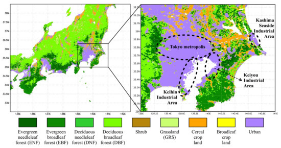
Figure 1.
Distribution of plant functional type (PFT) in the study area based on the MODIS land cover dataset (MCD12Q1, quality-control-screened) in 2018. Dashed cycles mark the Tokyo metropolis, Keihin Industrial Area, Keiyou Industrial Area, and Kashima Seaside Industrial Area, respectively.
To calculate the hourly 500 m × 500 m GPP and Re in the study area during the period 2010–2018, the MODIS LAI dataset (MCD15A3H v006 [107], 4-day 500 m), Land Cover Dynamics dataset (MCD12Q2 v006 [119], annual 500 m), and BRDF-derived Clumping Index [108] were applied to quantify the regional vegetation canopy structure after quality control screening (details are presented in the Supplementary Materials). The surface albedo was set by the MODIS albedo product (MCD43A3 v006 [109]). The fractions of clay, sand, and silt and the amount of organic carbon in the 0–200 cm soil layers were converted from the SoilGrids250m dataset [111]. Before March 2015, soil moisture and temperature data were based on the ERA-5 Land reanalysis dataset [110]. After March 2015, root zone soil moisture data were also extracted from the Soil Moisture Active Passive (SMAP) Root Zone (0–100 cm) Soil Moisture Geophysical Dataset (SMAPL4SMGPH v5 [120], 3-h 9 km) to calculate the effects of soil water availability on photosynthesis and to calculate the hydraulic limit of transpiration. Hourly surface air temperature, relative humidity, atmospheric pressure, wind speed, precipitation, cloud covers, and downward shortwave solar radiation in the MSM-GPV reanalysis dataset [112] were also processed as input data for the calculations. Depending on the data file format, the resampling of the input data to geographic projection was realized using the HDF-EOS to GeoTIFF Conversion Tool [121], Geospatial Data Abstraction Library [122] or wgrib2 [123]. Smoothing iteration in gdal_fillnodata.py [122] was applied to fill missing edge data of soil moisture or temperature. Similar to the modeling at the site level, a spin-up simulation was conducted regionally to initialize SOC in the study area: input data of the period 2010–2018 were used repeatedly until the carbon stock in the 0–28 cm soil layers (Figure S1 in the Supplementary Materials) reached approximately 6.95 ± 3.25 kg m−2 [116].
Furthermore, hourly modeling results were aggregated and compared to the MODIS Gross Primary Productivity (MOD/MYD17A2HGF v006 [124,125], 8-day 500 m), the Global OCO-2 Solar-Induced Chlorophyll Fluorescence (SIF) Gross Primary Production (GOSIF GPP [126], 8-day 5 km), and the MODIS Net Primary Production (MOD/MYD17A3HGF v006 [127,128], annual 500 m). By calculating the difference between the modeling output and existing satellite datasets, the performances of our GPP and Re model were analyzed further.
2.5. Estimation of Integrated Anthropogenic CO2 Emissions in the Greater Tokyo Area
Finally, the calculation results in Section 2.4 were compared with anthropogenic CO2 emissions data in the Greater Tokyo Area spatially and at various time scales. Annual anthropogenic CO2 emission data by sector (TotalEsector2018, e.g., construction, industry, agricultural waste burning, vehicle, ship, aircraft) in Japan in 2018 were obtained at as high a rate as possible from the national greenhouse gas emissions report provided by the Ministry of the Environment of Japan [129]. For our study area specifically, hourly human-induced CO2 emissions in January to December were estimated based on the East Asian Air Pollutant Emissions Grid Database (EAGrid2000Japan [130]), where the value of each grid cell by sector (GridCellEsectorEAGrid2000Japan) was adjusted using a constant ratio (fsector) of total CO2 emissions in 2000 to that in 2018:
fsector = TotalEsector2018/TotalEsector2000
GridCellEsector2018 = fsector × GridCellEsectorEAGrid2000Japan
In addition, integrated anthropogenic CO2 emission of all source sectors, GPP, Re, and NEE of the Greater Tokyo Area were calculated to elucidate the patterns of sub-daily and seasonal variations: the mean and standard deviation of biogenic integrated fluxes were calculated based on hourly results of all the days in each month during the period 2010–2018.
3. Results
3.1. Hourly GPP at the Site Level
Comparison between hourly modeled GPP and FFNet DB/FLUXNET2015 estimation provides reference information about the modeling uncertainty of CO2 uptake via photosynthesis in DBF, EBF, ENF, and GRS. As presented in Figure 2a (the evaluation metrics values also detailed in Table S2), the degree of similarity [131] between hourly GPPBEAMS (Big-Leaf upscaling scheme) and GPPtower was greater than 0.6 in both calibration and validation groups. Stated more specifically, the hourly GPPBEAMS agreed closely with GPPtower in ENF (R2 ≥ 0.75), followed by DBF (R2 ≥ 0.63), EBF (R2 ≥ 0.53), and GRS (R2 ≥ 0.49). The difference between flux tower-estimated and modeled standard deviation of hourly GPP at the site level was always within 1.22 μmolCO2 m−2 s−1, and therefore was acceptable. The RMSE of the hourly GPPBEAMS was less than 6.1 μmolCO2 m−2 s−1 or 0.26 gC m−2 h−1, where the largest was found for DBF and the smallest was found for GRS.
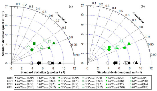
Figure 2.
(a) Taylor diagram of hourly modeled GPPBEAMS and hourly GPP estimates based on flux tower monitoring (μmol m−2 s−1) at selected FFNet DB/FLUXNET2015 sites. (b) Taylor diagram of hourly modeled GPPTLM and hourly GPP estimates based on flux tower monitoring (μmol m−2 s−1) at selected FFNet DB/FLUXNET2015 sites.
The accuracy of the hourly modeled GPPTLM (two-leaf upscaling scheme) was better than that of the hourly modeled GPPBEAMS when compared to GPPtower, but with one exception in the validation group of ENF (QIA). As with GPPBEAMS, the similarity between hourly GPPTLM and GPPtower was greater than 0.6 in both the calibration and validation groups, according to Figure 2b and Table S2. Hourly GPPTLM also showed very good agreement with GPPtower in ENF (R2 ≥ 0.74), DBF (R2 ≥ 0.67), EBF (R2 ≥ 0.61), and GRS (R2 ≥ 0.50). The difference between the flux tower estimated and modeled standard deviation of hourly GPP in the two-leaf module was within 1.05 μmolCO2 m−2 s−1, smaller than that in the case of GPPBEAMS. The RMSE of hourly GPPTLM was less than 5.55 μmolCO2 m−2 s−1, or 0.24 gC m−2 h−1, which was again smaller than the value of hourly GPPBEAMS.
3.2. Hourly Re and NEE at the Site Level
The comparison between hourly modeled Re and FFNet DB/FLUXNET2015 estimation provides reference information about the modeling uncertainty of CO2 emission via autotrophic and heterotrophic respiration in DBF, EBF, ENF, and GRS, as detailed in Figure 3a and Table S2. In DBF, ENF, and GRS, the hourly modeled Re agreed well with the Re estimates based on flux tower monitoring data (R2 ≥ 0.71, 0.52, and 0.66, respectively). In EBF, the calculated hourly Re agreed poorly with flux tower estimates at low latitude sites—DIN and PSO. At the mixed broadleaf forest site YMS in Japan, simulated hourly Re using both DBF and EBF parameters agreed well with flux tower-estimated Re (R2 was 0.68 and 0.76). In ecosystems of all four types, hourly Re was overestimated. The standard deviation of hourly modeled Re was 0.70–1.24 times (absolute difference within 0.66 μmolCO2 m−2 s−1 that of the flux tower estimated one. Consequently, the RMSE of hourly Re was up to 2.61 μmolCO2 m−2 s−1, or 0.11 gC m−2 h−1 in EBF, followed by ENF, DBF, and GRS, in descending order.
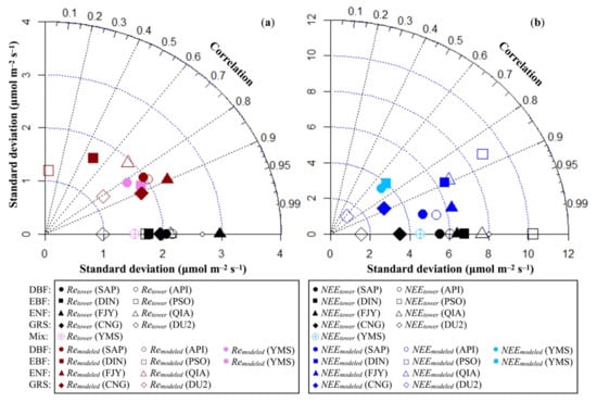
Figure 3.
(a) Taylor diagram of hourly modeled Re and hourly Re estimates based on flux tower monitoring (μmol m−2 s−1) at selected FFNet DB/FLUXNET2015 sites. (b) Taylor diagram of hourly modeled NEE (the difference of hourly modeled Re and GPPtower) and hourly NEE estimates based on flux tower monitoring (μmol m−2 s−1) at selected FFNet DB/FLUXNET2015 sites.
Hourly Re was approximately one to two thirds of hourly GPP in terms of the absolute value, while the former often presented much less sub-daily variations than the latter. As a result, their difference, hourly modeled NEE, agreed well with flux tower estimates at the site level simulations (Figure 3b and Table S2), though hourly modeled Re tended to be overestimated. In DBF, the correlation coefficient of hourly NEE was equal to or larger than 0.95, followed by ENF (R2 ≥ 0.79), EBF (R2 ≥ 0.74), and GRS (R2 ≥ 0.41). Contrary to the hourly modeled Re, the standard deviation of the hourly modeled NEE was only 0.80–0.98 times (the difference of the absolute values was within 1.33 μmolCO2 m−2 s−1) that of the flux tower estimated one. The RMSE of the hourly modeled NEE was up to 5.43 μmolCO2 m−2 s−1, or 0.23 gC m−2 h−1 in EBF, followed by ENF, DBF, and GRS, in descending order. The standard deviation of the hourly modeled NEE at YMS was close to that of the flux tower-estimated NEE, when assuming with either DBF or EBF parameters; the RMSE of the hourly modeled NEE was 3.21 and 3.37 μmolCO2 m−2 s−1, while the correlation coefficient was 0.51 and 0.50, respectively. These results might be partially attributable to the overestimation of hourly Re: overestimated Re can engender a positive NEE value, representing a false net carbon release, when the actual Re was smaller than GPP and there was actually net carbon uptake.
3.3. Hourly GPP at the Regional Scale
Because point-scale modelling results suggest that hourly modeled GPPTLM was close to or more accurate than hourly modeled GPPBEAMS, only the GPPTLM estimates at the regional scale were presented in the following analyses for simplicity, although regional simulations of the latter were conducted and generated similar results. Figure 4a–g present hourly GPP results of the study area from dawn to dusk on a summer day as examples of diurnal variations of vegetation CO2 uptake. Hourly GPP was generally low (<0.75 gC m−2 h−1) in the early morning because of the limited availability of solar radiation. By virtue of the favorable weather conditions (e.g., 20–34 °C air temperature, 0.5–0.9 soil moisture wetness) in the study area, as the level of shortwave solar radiation increased, the hourly GPP raised quickly (up to 1.5 gC m−2 h−1) and peaked before noon. Then, in the late afternoon, the hourly GPP dropped and became 0 after sunset. Spatially, the hourly GPP was up to 1.19 ± 0.27, 0.90 ± 0.18, and 0.93 ± 0.18 gC m−2 h−1 in ENF, EBF, and DBF, and 1.19 ± 0.39 gC m−2 h−1 in GRS, as the means and standard deviations of hourly GPP among all grid cells in Figure 6 show. In contrast, the hourly GPP was only up to 0.69 ± 0.19 gC m−2 h−1 in urban grid cells with partial vegetation cover.
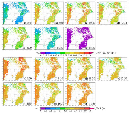
Figure 4.
Sub-daily variation of (a–g) hourly modeled GPP (gC m−2 h−1) and (h–n) hourly modeled fraction of APPFD by plant canopy (-) in the study area on 3 July 2018.
Depending on the distribution of cloud cover and vapor pressure, in cloudy summer periods with highly diffuse shortwave solar radiation ratios, plants in forests or grasslands effectively absorbed many of the available photosynthetically active photons, although the downward shortwave solar radiation was as low as 200–300 W m−2. Consequently, the hourly GPP in such cloudy conditions could reach 0.6–1.2 gC m−2 h−1. In raining areas, precipitation interfered with stomatal conductance of CO2 in photosynthesis, thereby temporarily reducing the hourly modeled GPP to 0. Over seasons, the range and spatial distribution of the hourly GPP varied according to the changes in meteorological and ecological conditions. Because of limited space, more examples of the hourly modeling results are not presented here.
In addition, Figure 4 also includes diurnal variations of the modeled fraction of absorbed PPFD on the same summer day. By virtue of the density of the leaf area in summer, the fraction of absorbed PPFD by the vegetation canopy was high (>0.7) in most of the forests in the study area but lower (0.2–0.6) in less densely vegetated urban grid cells. In agreement with earlier studies [57,132], this variable also exhibited diurnal change, higher in the early morning and late afternoon of a sunny day, when the ratio of diffuse PPFD was relatively high, as Figure 4h,i,m,n show.
3.4. Hourly Re at the Regional Scale
Figure 5 presents hourly Re results on the same summer day as in Figure 4 and Figure 6, to give examples of sub-daily variations of biogenic CO2 emission. At night, in evergreen forests in the southeast, northeast and west of the study area, hourly Re was strong (about 0.18 ± 0.06 to 0.22 ± 0.10 gC m−2 h−1), probably because of active microbial and chemical decomposition of SOC under favorable soil temperatures and moisture conditions, where litter carbon was abundant. In contrast, hourly Re was lower in DBF near the eastern coastline and in most urban grid cells with partial vegetated cover. The latter hourly Re was roughly 0.04 ± 0.01 gC m−2 h−1 according to Figure 6. In the daytime, the total of autotrophic and heterotrophic respiration in all types of ecosystem increased, up to 0.35 ± 0.13 gC m−2 h−1 in forests, 0.35 ± 0.27 gC m−2 h−1 in grassland, and 0.19 ± 0.06 gC m−2 h−1 in partially vegetated urban area. Diurnal temperature difference and additional growth respiration of plants to use photosynthesis-captured carbon most likely caused such a day–night difference of hourly Re.
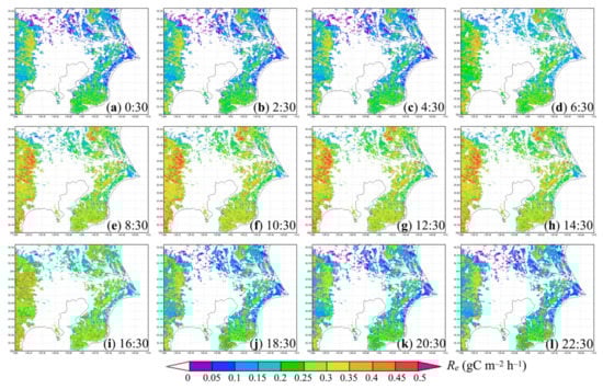
Figure 5.
Diurnal variation of (a–l) hourly modeled Re (gC m−2 h−1) in the study area on 3 July 2018.
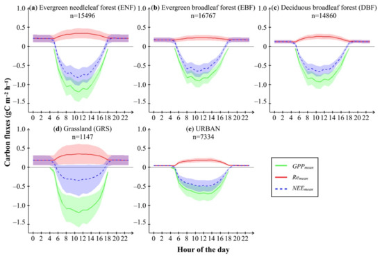
Figure 6.
Diurnal variation of hourly mean GPP, Re, and NEE (gC m−2 h−1) of (a) evergreen needleleaf forest, (b) evergreen broadleaf forest, (c) deciduous broadleaf forest, (d) grassland, and (e) partially vegetated urban land in the study area on 3 July 2018. Shadows represent the standard deviation of hourly GPP (green), Re (red), and NEE (blue), which were derived from modeled results in all grid cells of each PFT.
Hourly NEE (the difference of Re and GPP) in different types of ecosystem was also presented by the mean and standard deviation among all grid cells in Figure 6. At night, Re was the sole contributor of hourly NEE, and therefore the latter shared the same range of values described in the paragraph above. In the daytime, the strongest net carbon uptake occurred in ENF, up to –0.82 ± 0.22 gC m−2 h−1, followed by DBF, EBF, urban land with partial vegetated cover, and GRS, up to −0.66 ± 0.13, −0.65 ± 0.16, −0.49 ± 0.15, and −0.35 ± 0.41 gC m−2 h−1, respectively.
Furthermore, Table 3 summarizes the annual averaged GPP and Re during the period 2010–2018 in different types of ecosystem within the study area. According to our calculation, the highest annual averaged GPP occurred in ENF, about 1834.27 ± 38.60 gC m−2 year−1. By virtue of the longer photosynthetic active period in EBF than in DBF, the annual averaged GPP in EBF (1484.26 ± 22.22 gC m−2 year−1) was significantly higher than that in DBF (1254.42 ± 67.63 gC m−2 year−1), even though the hourly averaged GPP in these two types of broadleaf forest was similar from May to October. In GRS, the annual averaged GPP was 1409.33 ± 185.44 gC m−2 year−1. The annual averaged GPP in partially vegetated urban areas was 1020.77 ± 93.59 gC m−2 year−1, probably because of a less dense LAI level than that in forests or grassland. The strongest annual averaged Re occurred in GRS, about 1308.89 ± 280.83 gC m−2 year−1, followed by ENF, EBF, and DBF in descending order. The annual averaged Re in partially vegetated urban area was only 393.85 ± 38.41 gC m−2 year−1; both the limited SOC-decomposition-induced CO2 emissions and less dense LAI level probably caused this.
Table 3.
Annual averaged and integrated GPP and Re estimates in deciduous broadleaf forest (DBF), evergreen broadleaf forest (EBF), evergreen needleleaf forest (ENF), grassland (GRS), and partially vegetated urban area of the Greater Tokyo Area (139°E–141°E, 35°N–36.33°N) during the period 2010–2018.
3.5. Comparison of Regional Scale Modeling Results and Satellite Data
Hourly modeled GPP at the regional scale also presented clear seasonal changes. Figure 7a–d depict examples of 8-day sums of hourly modeled GPP from winter to autumn. Because little or no valid MODIS LAI was detected in the urban land close to the Tokyo bay in our study area year-round, GPP was zero there. In January, our model estimated up to 10.0 gC m−2 8-day−1 photosynthetic carbon uptake in deciduous forests and urban vegetated land. In contrast, GPP was almost 30.0 gC m−2 8-day−1 in evergreen forests, even in winter. When spring approached and temperatures increased, so did GPP in such evergreen forests. The GPP remained low in deciduous forests and some urban vegetated land, as the leaf area had not fully expanded yet. Summertime GPP was about 40.0–90.0 gC m−2 8-day−1 in ecosystems of all types because of favorable solar radiation and temperature conditions. It then decreased to 10.0–70.0 gC m−2 8-day−1 in autumn until leaf fall occurred.
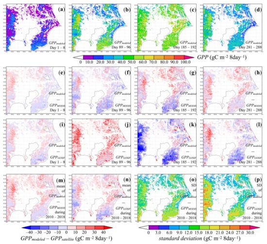
Figure 7.
Seasonal variation examples of (a–d) modeled 8-day GPP, (e–h) difference between modeled and MODIS (MOD17A2HGF) 8-day GPP, and (i–l) difference between modeled and GOSIF 8-day GPP in 2018; the average (m) and standard deviations (o) of the difference between modeled and MODIS (MOD17A2HGF) 8-day GPP during the period 2010–2018; the average (n) and standard deviations (p) of the difference between modeled and GOSIF 8-day GPP during the period 2010–2018.
The reason to calculate 8-day GPP of the study area was that few GPP datasets or reference values in earlier studies were available at the sub-daily scale. In fact, only Bodesheim et al. [133] has modeled global half-hourly biogenic CO2 flux data, but the spatial resolution (0.5°) of this dataset was too coarse to validate our modeling results. Therefore, comparisons between our 8-day GPP results and MODIS GPP [124,125] or GOSIF GPP [126] (Figure 7e–p) were presented. As Figure 7e-h show, our model estimated higher (0.0–30.0 gC m−2) 8-day GPP than the MODIS one in evergreen forests in the northeast and west of the study area. In contrast, the modeled 8-day GPP was 0.0–20.0 gC m−2 lower compared to MODIS 8-day GPP in the western deciduous forests and southeastern evergreen forests; for the latter, the discrepancy was up to 30.0 gC m−2 in summertime (Figure 7g). Over seasons, the range of difference was larger in summer than in winter while the spatial patterns remained the same, as the average and standard deviation of the difference between the modeled and MODIS 8-day GPP during the period 2010–2018 in Figure 7m-o indicate.
In January (Figure 7i) and October (Figure 7l), the difference between the modeled and GOSIF 8-day GPP was similar to the case of the modeled and MODIS 8-day GPP comparisons. Interestingly, GOSIF 8-day GPP was lower (up to 40.0 gC m−2) than our modeled results or MODIS GPP in April (Figure 7j), and then became much larger than the latter two estimates in July (Figure 7k). The favorable conditions (e.g., warm temperature and sufficient solar radiation) in spring and frequent rain in summer shaped the seasonal patterns of our modeled GPP, which probably led to the discrepancy with GOSIF 8-day GPP. The average and standard deviation of the difference between the modeled and GOSIF 8-day GPP during the period 2010–2018 are presented in Figure 7n–p. In addition to forests and partially vegetated urban area, MODIS GPP [124,125] also provides GPP estimates in agricultural land in the northeast of the study area that was not included in our simulations. GOSIF GPP [126] estimated a photosynthetic carbon uptake of 0–10.0 gC m−2 8-day−1 in winter and 10.0–30.0 gC m−2 8-day−1 in summer in the highly urbanized areas next to the Tokyo bay, which both our model and the MODIS GPP dataset considered non-vegetated.
In terms of NPP, our annual modeled NPP (Figure 8a) was about 0.6–2.0 kgC m−2 year−1 in forests and up to 0.6 kgC m−2 year−1 in urban vegetated land in 2018. Evergreen forests in particular presented high NPP, 1.2–2.0 kgC m−2 year−1, by virtue of a longer photosynthetic active period. Our modeled NPP was larger compared to annual MODIS NPP (Figure 8b,c) values, especially in evergreen forests in the northeast and west of the study area. This was probably because of lower estimates of autotrophic respiration and growth respiration rate of plants in particular, considering that the modeled GPP showed good agreement with MODIS GPP and that the algorithm of maintenance respiration in this study was similar to the MODIS method. Because of limited space, comparisons of 8-day GPP and annual NPP to satellite data in 2010–2017 are not presented, but were very similar to those obtained for cases of 2018.
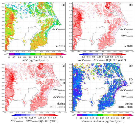
Figure 8.
Regional variation example of (a) modeled annual NPP and (b) difference between modeled and MODIS (MOD17A3HGF) annual NPP in 2018; the average (c) and standard deviations (d) of the difference between modeled and MODIS (MOD17A3HGF) annual NPP during the period 2010–2018.
3.6. Biogenic CO2 Fluxes and Anthropogenic CO2 Emissions in the Greater Tokyo Area
The spatial distribution of anthropogenic CO2 emissions and biogenic CO2 fluxes in the Greater Tokyo Area barely overlapped and exhibited some asynchronous characteristics, as the examples of our modeling results in Figure 4, Figure 5 and Figure 9 demonstrate. On one hand, Tokyo was surrounded by evergreen and deciduous forests in Ibaraki, Chiba, Saitama, and Kanagawa prefectures, which were sources of biogenic CO2. On the other hand, strong anthropogenic CO2 emissions occurred from the Tokyo metropolis, as well as from the Keihin and Keiyou industrial areas near Tokyo and the Kashima seaside industrial area (marked by dashed cycles in Figure 1, respectively), where power plants and factories are concentrated. If the range of the biogenic CO2 flux in our study area was much smaller than that of anthropogenic CO2 emissions, then neglecting the former in a top-down approach modeling would not cause much error in back-casting results. Otherwise, accurate calculation of the biogenic CO2 flux is essential for updating the anthropogenic CO2 emission inventory in the megacity of Tokyo. The comparisons of hourly integrated GPP (photosynthetic CO2 uptake), Re (biogenic CO2 emission), and NEE (net biogenic CO2 flux) to hourly anthropogenic CO2 emissions in the Greater Tokyo Area (Figure 10) provide some reference to evaluate this question. For our study, “hourly integrated” refers to the sum of modeled results in all grid cells within 139°E–141°E, 35°N–36.33°N, averaged over all days in each month during the period 2010–2018. The mean and standard deviation of hourly integrated biogenic CO2 fluxes are elaborated as below.
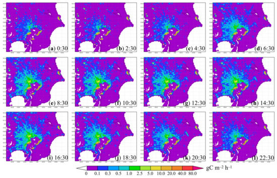
Figure 9.
Diurnal variation of (a–l) hourly estimated anthropogenic CO2 emission (gC m−2 h−1) in the study area in July 2018. The spatial distribution of emission was based on EAGrid2000Japan, adjusted by the annual emissions in 2018 published by the Ministry of the Environment of Japan.
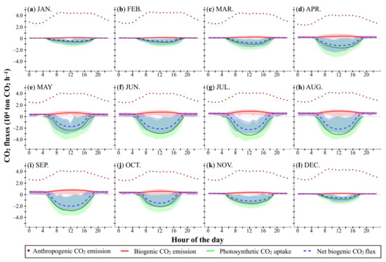
Figure 10.
(a–l) Hourly integrated anthropogenic CO2 emissions (104 ton CO2 h−1) in 2018, compared to hourly integrated biogenic CO2 emissions, photosynthetic CO2 uptake, and net biogenic CO2 flux of the Greater Tokyo Area (104 ton CO2 h−1) during the period 2010–2018. Shadows represent the variation (the minimum to the maximum) of hourly integrated biogenic CO2 emission (red), photosynthetic CO2 uptake (green), and net biogenic CO2 flux (blue).
To elaborate, first, hourly integrated anthropogenic CO2 emissions of the Greater Tokyo Area presented similar diurnal variations year-round; the lowest level (2.37–2.64 × 10⁴ ton CO2 h−1) was found after midnight when human activities were least active. As traffic rush hours started in the morning, hourly integrated anthropogenic CO2 emissions increased gradually and almost doubled by around 9 a.m. to 4.05–4.63 × 10⁴ ton CO2 h−1. From then until late afternoon, the integrated anthropogenic CO2 emissions entered a plateau phase and then started to drop at about 8 pm, after the evening traffic rush hours.
Secondly, the hourly integrated biogenic CO2 emissions of the Greater Tokyo Area, the total of vegetation-respired CO2 and CO2 emitted via SOC decomposition processes, exhibited both sub-daily and seasonal variations. At night, the lowest hourly integrated biogenic CO2 emissions (0.09 ± 0.01 × 10⁴ ton CO2 h−1), which was about 3.07 ± 0.51% of the hourly integrated anthropogenic CO2 emission in the area, occurred at 4 a.m. in January. In the daytime, the hourly integrated biogenic CO2 emissions became stronger and peaked in the early afternoon (around 3 p.m.). The peak biogenic CO2 emission (0.16 ± 0.03 × 10⁴ ton CO2 h−1) was equivalent to about 3.55 ± 0.79% of the hourly integrated anthropogenic CO2 emissions in January. Such a rise in integrated biogenic CO2 emissions was probably attributable to increased temperatures and additional vegetation growth respiration when photosynthesis was active during the day.
As meteorological conditions became more favorable for SOC decomposition from winter to summer and vegetation became more active in terms of both maintenance and growing activities, hourly integrated biogenic CO2 emissions of the Greater Tokyo Area increased considerably. In July, the lowest hourly integrated biogenic CO2 emissions were at 5 a.m. and was estimated to be 0.56 ± 0.08 × 10⁴ ton CO2 h−1, roughly 18.76 ± 2.80% of the hourly integrated anthropogenic CO2 emissions in the Greater Tokyo Area and 6.35 times the biogenic value in January. The strongest hourly integrated biogenic CO2 emissions were found at noon and were estimated to be 0.96 ± 0.13 × 10⁴ ton CO2 h−1, which was 6.39 times that of January’s biogenic level, and 23.62 ± 3.13% of the hourly integrated anthropogenic CO2 emissions, as the latter also increased after several hour.
Thirdly, hourly integrated photosynthetic CO2 uptake of the Greater Tokyo Area represents the amount of absorbed carbon by forests, grassland or urban vegetation, varying both diurnally and seasonally. Because the calculation of GPP in our model was under the assumption that the supply of CO2 for photosynthetic reactions in C3 plants is controlled by stomata in daytime only, the hourly integrated photosynthetic CO2 uptake at night was 0. In winter, the absolute value of hourly integrated photosynthetic CO2 uptake in both the early morning and late afternoon was low and was the lowest (0.04 ± 0.06 × 10⁴ ton CO2 h−1 and 1.34 ± 2.03% of the hourly integrated anthropogenic CO2 emissions in the Greater Tokyo Area) at 5 a.m. in January. Because photosynthetic enzymes became more active at higher winter temperatures and because more photosynthetically active radiation was available around midday, the hourly integrated photosynthetic CO2 uptake was enhanced. For January, the highest absolute value was obtained around 2 p.m., and that value (0.62 ± 0.17 × 10⁴ ton CO2 h−1) was 14.08 ± 3.89% of the hourly integrated anthropogenic CO2 emissions. As the seasons changed, hourly integrated photosynthetic CO2 uptake of the Greater Tokyo Area reached the highest level in July, with an absolute value of 3.22 ± 0.50 × 10⁴ ton CO2 h−1 at noon and 5.42 times the January value. This amount was 79.04 ± 12.31% of the hourly integrated anthropogenic CO2 emissions.
Finally, the hourly integrated net biogenic CO2 flux of the Greater Tokyo Area represents the amount of CO2 flow from ecosystems to the atmosphere. At night, such flow was one-way, from forests, grasslands, and urban vegetated areas into the air. The nighttime vegetated land of the Greater Tokyo Area was a natural carbon source, collectively emitting 0.08 ± 0.01 × 10⁴ to 0.09 ± 0.01 × 10⁴ ton CO2 h−1 in January and 0.56 ± 0.09 × 10⁴ to 0.60 ± 0.10 × 10⁴ ton CO2 h−1 in July, which were 3.07 ± 0.51% to 2.34 ± 0.41% and 21.97 ± 3.38% to 17.80 ± 2.97% of the hourly integrated anthropogenic CO2 emissions for January and July, respectively. Depending on whether the photosynthetic CO2 uptake would completely compensate for the biogenic CO2 emission in each grid cell or not, the daytime net biogenic CO2 flux from ecosystems to the atmosphere was either negative or positive. Here, negative net biogenic CO2 flux values mean that the direction of carbon flow is reversed (from atmosphere to the ecosystem): a natural carbon sink. The maximal negative hourly integrated net biogenic CO2 flux of the Greater Tokyo Area often occurred around 12 a.m. to 2 p.m. in all seasons, −0.46 ± 0.14 × 10⁴ ton CO2 h−1 in January in winter to −2.26 ± 0.42 × 10⁴ ton CO2 h−1 in July in summer, would potentially offset 10.52 ± 3.17% to 55.42 ± 10.39% of the hourly anthropogenic emissions.
Overall, the sub-daily patterns of hourly integrated biogenic CO2 emissions, photosynthetic CO2 uptake, and net biogenic CO2 flux of the Greater Tokyo Area were bell-shaped, whereas the ranges of hourly integrated values increased from winter to spring and from spring to summer, subsequently dropping in autumn. The intraday peaks almost always occurred around midday, but the highest hourly integrated biogenic CO2 emissions often appeared several hours later than the photosynthetic CO2 uptake. In each month, the variation of hourly integrated photosynthetic CO2 uptake of the Greater Tokyo Area was much greater than that of biogenic CO2 emissions. As a result, the integrated net biogenic CO2 flux fluctuated between positive and negative figures within a day.
Figure 11 presents the integrated anthropogenic CO2 emissions, biogenic CO2 emissions, photosynthetic CO2 uptake, and net biogenic CO2 flux of the Greater Tokyo Area at the monthly scale. In winter to early spring (December to March), the integrated biogenic CO2 flux was lower than the anthropogenic one by more than one order of magnitude (the ratio of integrated biogenic CO2 flux to anthropogenic emission was only 3.34 ± 0.54% in February). From April to November, both photosynthesis and biogenic respiration became more active, up to 34.29 ± 5.92% and 20.46 ± 1.96% of the integrated anthropogenic CO2 emissions. Consequently, the integrated biogenic CO2 flux was up to 17.06 ± 5.44% of the anthropogenic one in June.
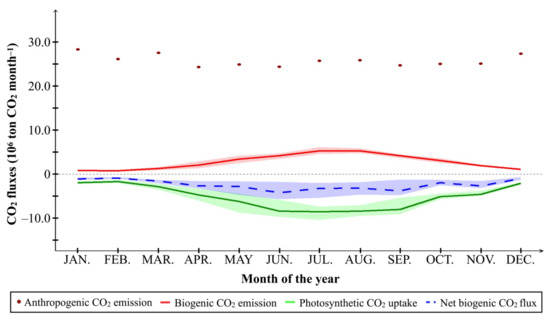
Figure 11.
Monthly integrated anthropogenic CO2 emissions (106 ton CO2 month−1) in 2018, compared to biogenic CO2 emissions, photosynthetic CO2 uptake, and net biogenic CO2 flux of the Greater Tokyo Area (106 ton CO2 month−1) during the period 2010–2018. Shadows represent the variation (the minimum to the maximum) of monthly integrated biogenic CO2 emission (red), photosynthetic CO2 uptake (green), and net biogenic CO2 flux (blue).
4. Discussion
The sub-daily scale terrestrial biosphere model developed for this study was based on earlier studies [55,69,88]. It required multiple satellite datasets as input. Our main motivation of GPP and Re simulation in such short time-steps was to disaggregate biogenic CO2 fluxes from the anthropogenic CO2 emissions of the Tokyo megacity and surrounding industrial areas in future inversion studies. Even though some driving forces of the model (i.e., temperature, solar radiation, and soil moisture data) are available hourly or every few hours, sub-daily scale modeling of biogenic CO2 flux remained challenging.
In terms of GPP calculation, earlier satellite-based models often applied the light use efficiency concept [71,72], which requires APPFD by plant canopy or its equivalent in W m−2 as input. However, global daily satellite datasets to calculate APPFD, let alone sub-daily ones, are not available yet. Furthermore, after removing cloud-contaminated points, valid data obtained from existing dataset such as MODIS 4-day LAI/Fraction of Photosynthetically Active Radiation ([107]) are incomplete, especially in regions such as our study area, where the rain period is long in summer. To prepare complete and continuous hourly APPFD estimates for GPP calculation, we introduced the satellite-derived clumping index Ω and interpolated LAI as the input. An ANN was also trained to estimate hourly diffuse shortwave solar radiation under various weather conditions. This combination allowed the generalization of APPFD modeling method proposed in de Pury and Farquhar [55]. Because both diffuse and direct PPFD were accounted for in hourly APPFD modeling processes, underestimation of GPP [51] was alleviated in our model. It also means simulating more realistic diurnal variations of photosynthetic CO2 uptake compared to existing terrestrial biosphere models, for instance, VPRM [43,48,49], which were applied in the field of top-down CO2 emissions verification studies at a city scale.
Accurate temporal variation and spatial distribution of both LAI and the clumping index are the key to obtaining more realistic hourly APPFD estimates and subsequently more realistic hourly GPP. For this study, we set the clumping index of vegetated land to fixed values [108], assuming that the temporal variation of Ω was small within a growing season [57] and interannually (2010–2018). This assumption reflected a compromise because of dataset accessibility: it should be improved for future studies by introducing a clumping index dataset with finer temporal resolution, such as the Global Vegetation Clumping Index Products LIS-CI-A1 [134]. Until daily satellite LAI datasets become accessible, improvements to LAI data quality rely on better interpolation and smoothing algorithms. By introducing a satellite dataset of phenological metrics [119], we were able to smooth trends of 4-day LAI in deciduous forest and grassland areas. However, it is difficult to constrain satellite-observed LAI in evergreen forests by checking against date of vegetation green-up or dormancy. Our results of both hourly modeled GPP at the site level and comparison to existing GPP data at the regional scale suggest that temporal linear averaging interpolated LAI of evergreen forests was sufficient for accurate simulation of hourly GPP. However, frequently fluctuated LAI in evergreen forests can be expected to trigger abnormal amounts of leaf litter fall, which can lead to overestimation of SOC and risks of overestimating hourly Re. In this case, data assimilation of LAI [135,136,137,138,139] might provide an alternative for model improvement in future work.
Additionally, we recognized that in recent years, satellite-observed SIF has become a promising proxy for GPP because the two variables presented a strong linear relation [140,141,142]. Although we already used a SIF-based GPP dataset [126] to assess our modeled GPP results, it was difficult to apply this type of SIF-based GPP algorithm directly at sub-daily scale modeling because of similar challenges discussed in earlier paragraphs: temporally continuous, sub-daily SIF satellite datasets are not yet available. The ECOsystem Spaceborne Thermal Radiometer Experiment on Space Station (ECOSTRESS) and the Orbiting Carbon Observatory-3 (OCO-3) aboard the International Space Station (ISS) have diurnal sampling capability to some extent. ECOSTRESS has been used to develop instantaneous GPP estimates for different times of day [143], but neither ECOSTRESS nor OCO-3 could provide temporally continuous observations throughout the day due to the orbit nature of the ISS. Consequently, the diurnal variability of GPP cannot be simulated accordingly [144,145].
Because GPP modeling in this study was process-based, our last discussion point about photosynthetic CO2 removal estimation is about PFT-specific parameters. Following Wullschleger [76], we assumed that, in each PFT, the maximal electron transport rate Jmax in photosynthetic reactions was linearly related to the maximal carboxylation rate at 25 °C Vcmax25, where the latter was set as a constant. However, studies such as that by Kosugi et al. [146] observed a seasonal change in Vcmax25, which has been reflected in some global GPP models [147] and which should be included in our future model optimizations. Furthermore, the values of empirical parameters to calculate Vcmax25 based Jmax reported by Medlyn et al. [148] and Walker et al. [149] differ from those reference settings [76] for this study, which should be compared in further sensitivity tests of our GPP modeling.
In terms of Re modeling, hourly Re calculations in this study considered the effects of biomass amount in all vegetation biomass pools and SOC pools [69,70,86,87,88] instead of simple Re correlations to ambient temperature and soil moistures. This consideration is both a benefit and a challenge of our model because below-ground biomass was rarely obtained via satellite observations, if not impossible. Hourly modeled Re results at the site level suggest that our sub-daily model tended to overestimate biogenic CO2 emissions, which led to an overestimated natural carbon source at night and underestimated negative biogenic CO2 flux during the day.
Several parts of the hourly Re model might contribute to such results. To start with, we assumed that live-wood and root biomass were proportional to the foliage biomass in most cases (except for root biomass in DBF) for the allocation of hourly NPP, with a fixed specific leaf area (SLA) setting [82] in each PFT. Our forest NPP results fluctuate above or below the calculated values presented by Sasai et al. [69]: 1200 gC m−2 year−1 NPP in 1982–2000. These results also exceed the estimates of Ise et al. [150]. In that study, NPP of temperate forest was no more than 500 gC m−2 year−1. Occasionally, because the change in biomass was only constrained using the difference of LAI over time, carbon flow in and out of the plants was not fully balanced. This imbalance can cause errors of maintenance respiration and then biogenic CO2 emissions. To reduce modeling errors of this type, the data quality of the input LAI should be improved, as discussed in earlier paragraphs. Additionally, more representative values of PFT-specific parameters should be updated from the latest literature or from research datasets such as the TRY Plant Trait Database [151]. Another point to be addressed in future work is the assumption about growth respiration. Bruggemann et al. [152] reviewed existing isotope studies of plant and pointed out a time lag of transport and allocation of carbon from leaves to the root tissues belowground, suggesting that our assumption of almost instantaneous GPP export to root utilization should be converted to a lagged one once measurement data are available to set the delay time range.
In addition to temperature and moisture conditions, initial SOC amounts also greatly affected the heterotrophic part of hourly Re. On one hand, active soil biomass pools such as SOCsurfacemetabolic, SOCsurfacemicrobe, SOCrootmetabolic, and SOCsoilmicrobe reached equilibrium (annual carbon change remained several grams or even larger by our calculations) rapidly during the spin-up. On the other hand, it would take more than one thousand years to stabilize SOCsoilpassive. However, hourly Re estimates based on these fully stabilized initial SOC settings were almost twice those of observed ones. Thereby, the number of years for spin-up was shortened to reduce SOC and Rheterotrophic overestimation.
To improve this aspect of modeling further, a few aspects must be addressed. As reported by Fierer et al. [153] and by Pugh et al. [154], both the quantity and quality of litter can be expected to affect the biomass amount in SOC and its decomposition rate. Estimating the hourly litter fall rate more accurately requires good estimation of plant biomass change in foliage, wood, and root parts, as described above. However, plant biomass loss attributable to biogenic volatile organic compound (VOC) emission [152], herbivore consumption [155], and litter loss because of dissolved carbon [64] should be updated or tuned to more accurately estimate SOC. From a quality perspective, PFT-specific parameters such as the lignin fraction and the lignin:nitrogen ratio can be further calibrated or adjusted with reference values from the TRY Plant Trait Database [151]. Our Re modeling only included carbon cycling, and coupling C and N might improve the simulations [85,87,88].
Because of the limited availability of GPP, Re, and NEE datasets for Japanese forests and grasslands, some (n = 5) flux tower sites’ data outside our study area and the 33°N–38°N range were used in model calibration and validation experiments. To improve the representativeness of model calibration, future availability of data from more observational sites is expected to reduce site-specific errors [133]. This point also addresses future application of our sub-daily scale model to provide fine-resolution biogenic CO2 flux data in an inversion analysis of anthropogenic CO2 emissions of other megacities, which requires both globally available satellite input datasets and well-tuned model parameters.
Furthermore, although biogenic CO2 fluxes induced by urban forest and greenspace were estimated in our sub-daily scale model, these calculations were based on natural vegetation parameters because of the scarcity of observational data. Such assumptions should be replaced in future work because urban vegetated land might present unique characteristics that are different from natural forests [49,156]. Although CO2 emissions attributable to agricultural biomass waste burning were counted in the anthropogenic emission data [129,130] that we used, photosynthetic CO2 uptake and crop-soil CO2 emissions in agricultural systems distributed in our study area were not included and could potentially be calculable based on a model described by Sasai et al. [157].
According to our hourly integrated biogenic CO2 emission, photosynthetic CO2 uptake and net biogenic CO2 flux results discussed in Section 3.6, the range of integrated hourly biogenic to anthropogenic CO2 emissions ratio in winter (2.27 ± 0.11%–4.97 ± 1.17%) was similar to the value (4–5%) estimated in earlier urban CO2 flux studies [24,42,158]. However, the modeled ratio range in summer (13.71 ± 2.44%–23.62 ± 3.13%) was much higher than reference values, probably because our study area included much more vegetated land than Los Angeles [24], or a higher vegetation fraction than the neighborhood-scale studies in Singapore and Mexico City [42,158].
In terms of CO2 removal, the range of integrated hourly photosynthetic uptake to anthropogenic CO2 emission ratio in winter (up to 19.07 ± 5.33%) was comparable to the series of 1.4% in Velasco et al. [158], 8% in Velasco et al. [42], 10% in Brioude et al. [24], 14% in Hardiman et al. [49], and 20–24% in Park et al. [159]. In summer, the ratio of photosynthetic uptake to anthropogenic emissions (79.04 ± 12.31%) was higher than the estimate (69%) for a July afternoon in Boston [29]. The summer daytime integrated hourly net biogenic to anthropogenic CO2 flux ratio (up to 55.42 ± 10.39%) was higher than the 20% offset by daytime NEE in Paris [33] and up to 31% estimated by Menzer et al. [41] while our winter daytime estimates was only up to 14.15 ± 4.24%. Forests, grasslands, and urban greenspaces in the Greater Tokyo Area showed potential to offset Tokyo’s anthropogenic CO2 emissions, especially during the growing season.
According to Table 3, our model estimated 5.14 ± 0.47 × 10⁶ tonCO2 year−1 of photosynthetic uptake and 1.98 ± 0.19 × 10⁶ tonCO2 year−1 of biogenic emission in the partially vegetated urban land (1374.62 ± 134.05 km2) in the Greater Tokyo Area. Another 1665.31 km2 of urban land in the study area was also identified as having partial vegetation cover by the MODIS vegetation continuous fields product (MOD44B), but was without valid LAI data to proceed any simulation. Additionally, if the rest of the urban land (about 7065.07 km2) in our study area was fully covered by DBF, EBF, ENF or GRS instead, 3.25 ± 0.18 × 10⁷, 3.84 ± 0.06 × 10⁷, 4.75 ± 0.10 × 10⁷ or 3.64 ± 0.49 × 10⁷ ton year−1 more CO2 would be captured by photosynthesis, while 1.73 ± 0.19 × 10⁷, 2.08 ± 0.21 × 10⁷, 2.68 ± 0.27 × 10⁷ or 3.37 ± 0.71 × 10⁷ ton year−1 more CO2 would be emitted via biogenic respiration and SOC decomposition. Nonetheless, one must bear in mind that once the spatial range of hourly integrated calculation changed, so would the results [49,160]. These values were the total of GPP, Re, and NEE in ecosystems of different types under various environmental conditions. It is too complicated to make an interpretation without discussing factors such as near-ground CO2 storage [161,162,163], which affect the actual biogenic offset of anthropogenic CO2 emissions. For that reason, the gridded estimates of sub-daily biogenic CO2 flux are supplied to the transport model AIST-MM for inversion analysis of anthropogenic CO2 emissions in cities such as Tokyo.
5. Conclusions
Sub-daily photosynthetic CO2 uptake and biogenic CO2 emissions in DBF, EBF, ENF, GRS, and urban vegetated lands located in Tokyo and its surrounding areas were estimated via a terrestrial biosphere model driven by multiple satellite inputs and meteorological datasets. After calibrations, our modeled results were found to be consistent with both point-scale observed values and existing satellite-based data. The order of hourly integrated photosynthetic CO2 uptake and NEE values in the Greater Tokyo Area was up to about 80%, or approximately half of the total anthropogenic CO2 emissions in summer, and lower than one-tenth of the human-induced values in winter. Such modeling results not only provide reference data for the estimation of total natural CO2 removal in our study area but also provide prior input values for the disaggregation of anthropogenic CO2 emission and biogenic CO2 flux when applying top-down approaches to update the megacity’s CO2 emissions inventory. This allows for unprecedented amounts of GOSAT and ground measurement data of CO2 concentrations to be analyzed using inverse modeling of anthropogenic CO2 emissions from Tokyo and the Greater Tokyo Area. The updated megacity CO2 emissions inventory based on observations of CO2 concentration will serve to detect changes in emission and to improve the understanding of source patterns over space and time. The updating of the urban CO2 emissions inventory will also support the assessment of emission reduction efforts pledged and implemented by cities such as Tokyo.
Supplementary Materials
The following are available online at https://www.mdpi.com/article/10.3390/rs13112037/s1, Figure S1: Accumulated carbon (sum of SOCrootstructural, SOCrootmetabolic, SOCsoilmicrobe, SOCsoilslow, and SOCsoilpassive) (kgC m−2) in the 0–28 cm soil layer of the study area after model spin-up; Figure S2: Structure, layers, and nodes of artificial neural network (ANN) to estimate Ktdiffuse; Figure S3: Taylor diagram of hourly observed and modeled SRtdiffuse (W m−2) at the World Radiation Data Centre Fukuoka, Sapporo, and Tateno sites. Table S1: List of variables and their acronyms used in the sub-daily GPP, Re, and NEE model; Table S2: Evaluation metrics for model calibration and validation of hourly gross primary production (GPP), ecosystem respiration (Re), and net ecosystem exchange (NEE); Table S3: Parameters to activate the ANN and predict Ktdiffuse; Table S4: PFT-specific parameters used to calculate hourly Rmaintenance. References [164,165,166,167,168,169,170,171,172,173,174,175] are cited in the Supplementary Materials.
Author Contributions
Conceptualization, R.I.; methodology, Q.W., Y.A. and S.I.; software, Q.W., Y.A. and S.I.; validation, Q.W. and Y.A.; formal analysis, Q.W. and Y.A.; investigation, Q.W., Y.A. and S.I.; resources, R.I. and Y.M.; data curation, Q.W., Y.A. and S.I.; writing—original draft preparation, Q.W.; writing—review and editing, R.I., Y.M., H.K. and J.X.; visualization, Q.W. and Y.A.; supervision, R.I.; project administration, R.I.; funding acquisition, R.I. All authors have read and agreed to the published version of the manuscript.
Funding
This research received no external funding.
Data Availability Statement
The data presented in this study are available on request from the corresponding author.
Acknowledgments
We thank Takahiro Sasai for his useful comments about this study. We are grateful to Nobuko Saigusa (National Institute for Environmental Studies) and Akihiko Ito (National Institute for Environmental Studies) for their valuable comments on model development. We appreciate Yukio Yasuda (PI of FFNet DB Appi site), Satoru Takanashi (PI of FFNet DB Fuji Yoshida site and FluxNet2015 MY-PSO site), Takafumi Miyama (PI of FFNet DB Fuji Yoshida site), Katsumi Yamanoi (PI of FFNet DB Sapporo site), Yuji Kominami (PI of FFNet DB Yamashiro site), Gang Dong (PI of FluxNet2015 Cn-CNG site), Guoyi Zhou and Junhua Yan (PIs of FluxNet2015 Cn-DIN site), Shiping Chen (PIs of FluxNet2015 Cn-DU2 site), Yoshiko Kosugi (PI of FluxNet2015 MY-PSO site), Huimin Wang and Xiaoli Fu (PIs of FluxNet2015 Cn-Qia site) for the accessibility of flux tower GPP, Re, NEE, and meteorological data for model calibrations and validations. We are also grateful to the providers of MODIS, SMAP, ERA5-Land hourly data, SoilGrids250m, GOSIF GPP, and World Radiation Data Centre datasets. We thank the three anonymous reviewers for their constructive comments that improved the manuscript. The first author would like to acknowledge the Graduate Program in Sustainability Science—Global Leadership Initiative at the University of Tokyo for the fellowship to undertake her PhD.
Conflicts of Interest
The authors declare that they have no conflict of interest.
References
- World Meteorological Organization. The state of greenhouse gases in the atmosphere based on global observations through 2018. In WMO Greenhouse Gas Bulletin; WMO: Geneva, Switzerland, 2019. [Google Scholar]
- Friedlingstein, P.; Jones, M.; O’sullivan, M.; Andrew, R.; Hauck, J.; Peters, G.; Bakker, O.D. Global carbon budget 2019. Earth Syst. Sci. Data 2019, 11, 1783–1838. [Google Scholar] [CrossRef]
- De Cola, P.; Secretariat, W.M.O. An integrated global greenhouse gas information system (IG3IS). WMO Bull. 2017, 66, 38–45. [Google Scholar]
- United Nations, Department of Economic and Social Affairs. World Urbanization Prospects: The 2018 Revision (ST/ESA/SER.A/420); United Nations: New York, NY, USA, 2019. [Google Scholar]
- Churkina, G.; Brown, D.G.; Keoleian, G. Carbon stored in human settlements: The conterminous United States. Glob. Chang. Biol. 2010, 16, 135–143. [Google Scholar] [CrossRef]
- Duren, R.M.; Miller, C.E. Measuring the carbon emissions of megacities. Nat. Clim. Chang. 2012, 2, 560–562. [Google Scholar] [CrossRef]
- Creutzig, F.; Lohrey, S.; Bai, X.; Baklanov, A.; Dawson, R.; Dhakal, S.; Walsh, B. Upscaling urban data science for global climate solutions. Glob. Sustain. 2019. [Google Scholar] [CrossRef]
- Nagendra, H.; Bai, X.; Brondizio, E.S.; Iwasa, S. The urban south and the predicament of global sustainability. Nat. Sustain. 2018, 1, 341–349. [Google Scholar] [CrossRef]
- Arioli, M.S.; Márcio de Almeida, D.A.; Amaral, F.G.; Cybis, H.B.B. The evolution of city-scale GHG emissions inventory methods: A systematic review. Environ. Impact Assess. 2020, 80, 106316. [Google Scholar] [CrossRef]
- City of Los Angeles. 2017 Municipal Greenhouse Gas Emissions Inventory; LA Sanitation & Environment Regulatory Affairs Division, Climate Action Program: Los Angeles, CA, USA, 2017. [Google Scholar]
- Ville de Paris. Bilan des Emissions de Gaz à Effet de Serre de Paris; l’Agence d’Écologie Urbaine de la Direction des Espaces Verts et de l’Environnement: Paris, France, 2020. [Google Scholar]
- Bureau of Environment, Tokyo Metropolitan Government. Final Energy Consumption and Greenhouse Gas Emissions in Tokyo (FY2017); Bureau of Environment, Tokyo Metropolitan Government: Tokyo, Japan, 2020.
- Gurney, K.R.; Razlivanov, J.; Song, Y.; Zhou, Y.; Benes, B.; Abdul-Massih, M. Quantification of fossil fuel CO2 emissions on the building/street scale for a large US city. Environ. Sci. Technol. 2012, 46, 12194–12202. [Google Scholar] [CrossRef]
- Shan, Y.; Guan, D.; Liu, J.; Mi, Z.; Liu, Z.; Liu, J.; Zhang, Q. Methodology and applications of city level CO2 emission accounts in China. J. Clean. Prod. 2017, 161, 1215–1225. [Google Scholar] [CrossRef]
- Nangini, C.; Peregon, A.; Ciais, P.; Weddige, U.; Vogel, F.; Wang, J.; Yamagata, Y. A global dataset of CO2 emissions and ancillary data related to emissions for 343 cities. Sci. Data 2019, 6, 180280. [Google Scholar] [CrossRef]
- Dodman, D. Blaming cities for climate change? An analysis of urban greenhouse gas emissions inventories. Environ. Urban. 2009, 21, 185–201. [Google Scholar] [CrossRef]
- Bai, X.; Dawson, R.J.; Ürge-Vorsatz, D.; Delgado, G.C.; Barau, A.S.; Dhakal, S.; Schultz, S. Six research priorities for cities and climate change. Nat. Comment 2018. [Google Scholar] [CrossRef]
- Buendia, E.C.; Tanabe, K.; Kranjc, A.; Baasansuren, J.; Fukuda, M.; Ngarize, S.; Federici, S. 2019 Refinement to the 2006 IPCC Guidelines for National Greenhouse Gas Inventories; IPCC: Geneva, Switzerland, 2019; Volume 5, p. 194. [Google Scholar]
- Saeki, T.; Maksyutov, S.; Saito, M.; Valsala, V.; Oda, T.; Morino, I. Inverse modeling of CO2 fluxes using GOSAT data and multi-year ground-based observations. Sola 2013, 9, 45–50. [Google Scholar] [CrossRef]
- Houweling, S.; Baker, D.; Basu, S.; Boesch, H.; Butz, A.; Chevallier, F.; Hasekamp, O. An intercomparison of inverse models for estimating sources and sinks of CO2 using GOSAT measurements. J. Geophys. Res. Atmos. 2015, 120, 5253–5266. [Google Scholar] [CrossRef]
- Basu, S.; Baker, D.F.; Chevallier, F.; Patra, P.K.; Liu, J.J.; Miller, J.B. The impact of transport model differences on CO2 surface flux estimates from OCO-2 retrievals of column average CO2. Atmos. Chem. Phys. 2018, 18, 7189–7215. [Google Scholar] [CrossRef]
- McKain, K.; Wofsy, S.C.; Nehrkorn, T.; Eluszkiewicz, J.; Ehleringer, J.R.; Stephens, B.B. Assessment of ground-based atmospheric observations for verification of greenhouse gas emissions from an urban region. Proc. Natl. Acad. Sci. USA 2012, 109, 8423–8428. [Google Scholar] [CrossRef]
- Nehrkorn, T.; Henderson, J.; Leidner, M.; Mountain, M.; Eluszkiewicz, J.; McKain, K.; Wofsy, S. WRF simulations of the urban circulation in the Salt Lake City area for CO2 modeling. J. Appl. Meteorol. Clim. 2013, 52, 323–340. [Google Scholar] [CrossRef]
- Brioude, J.; Angevine, W.M.; Ahmadov, R.; Kim, S.W.; Evan, S.; McKeen, S.A.; Peischl, J. Top-down estimate of surface flux in the Los Angeles Basin using a mesoscale inverse modeling technique: Assessing anthropogenic emissions of CO, NOx and CO2 and their impacts. Atmos. Chem. Phys. 2013, 13, 3661–3677. [Google Scholar] [CrossRef]
- Feng, S.; Lauvaux, T.; Newman, S.; Rao, P.; Ahmadov, R.; Deng, A.; Gurney, K.R. Los Angeles megacity: A high-resolution land–atmosphere modelling system for urban CO2 emissions. Atmos. Chem. Phys. 2016, 16. [Google Scholar] [CrossRef]
- Turnbull, J.C.; Sweeney, C.; Karion, A.; Newberger, T.; Lehman, S.J.; Tans, P.P.; Cambaliza, M.O. Toward quantification and source sector identification of fossil fuel CO2 emissions from an urban area: Results from the INFLUX experiment. J. Geophys. Res. Atmos. 2015, 120, 292–312. [Google Scholar] [CrossRef]
- Lauvaux, T.; Miles, N.L.; Deng, A.; Richardson, S.J.; Cambaliza, M.O.; Davis, K.J.; Song, Y. High-resolution atmospheric inversion of urban CO2 emissions during the dormant season of the Indianapolis Flux Experiment (INFLUX). J. Geophys. Res. Atmos. 2016, 121, 5213–5236. [Google Scholar] [CrossRef] [PubMed]
- Turnbull, J.C.; Karion, A.; Davis, K.J.; Lauvaux, T.; Miles, N.L.; Richardson, S.J.; Patarasuk, R. Synthesis of urban CO2 emission estimates from multiple methods from the Indianapolis Flux Project (INFLUX). Environ. Sci. Technol. 2018, 53, 287–295. [Google Scholar] [CrossRef] [PubMed]
- Sargent, M.; Barrera, Y.; Nehrkorn, T.; Hutyra, L.R.; Gately, C.K.; Jones, T.; Wang, J.A. Anthropogenic and biogenic CO2 fluxes in the Boston urban region. Proc. Natl. Acad. Sci. USA 2018, 115, 7491–7496. [Google Scholar] [CrossRef] [PubMed]
- Hu, C.; Griffis, T.J.; Lee, X.; Millet, D.B.; Chen, Z.; Baker, J.M.; Xiao, K. Top-down constraints on anthropogenic CO2 emissions within an agricultural-urban landscape. J. Geophys. Res. Atmos. 2018, 123, 4674–4694. [Google Scholar] [CrossRef]
- Lopez-Coto, I.; Ren, X.; Salmon, O.E.; Karion, A.; Shepson, P.B.; Dickerson, R.R.; Whetstone, J.R. Wintertime CO2, CH4, and CO Emissions Estimation for the Washington, DC–Baltimore Metropolitan Area Using an Inverse Modeling Technique. Environ. Sci. Technol. 2020, 54, 2606–2614. [Google Scholar] [CrossRef]
- Lauvaux, T.; Miles, N.L.; Richardson, S.J.; Deng, A.; Stauffer, D.R.; Davis, K.J.; DeCola, P.L. Urban emissions of CO2 from Davos, Switzerland: The first real-time monitoring system using an atmospheric inversion technique. J. Appl. Meteorol. Clim. 2013, 52, 2654–2668. [Google Scholar] [CrossRef]
- Bréon, F.M.; Broquet, G.; Puygrenier, V.; Chevallier, F.; Xueref-Remy, I.; Ramonet, M.; Ciais, P. An attempt at estimating Paris area CO2 emissions from atmospheric concentration measurements. Atmos. Chem. Phys. 2015, 15. [Google Scholar] [CrossRef]
- Staufer, J.; Broquet, G.; Bréon, F.M.; Puygrenier, V.; Chevallier, F.; Xueref-Rémy, I.; Perrussel, O. The first 1-year-long estimate of the Paris region fossil fuel CO2 emissions based on atmospheric inversion. Atmos. Chem. Phys. 2016, 16, 14703–14726. [Google Scholar] [CrossRef]
- Pillai, D.; Buchwitz, M.; Gerbig, C.; Koch, T.; Reuter, M.; Bovensmann, H.; Burrows, J.P. Tracking city CO2 emissions from space using a high-resolution inverse modeling approach: A case study for Berlin, Germany. Atmos. Chem. Phys. 2016, 16, 9591–9610. [Google Scholar] [CrossRef]
- Klausner, T.; Mertens, M.; Huntrieser, H.; Galkowski, M.; Kuhlmann, G.; Baumann, R.; Helmig, D. Urban greenhouse gas emissions from the Berlin area: A case study using airborne CO2 and CH4 in situ observations in summer 2018. Elem. Sci. Anthr. 2020, 8. [Google Scholar] [CrossRef]
- Boon, A.; Broquet, G.; Clifford, D.J.; Chevallier, F.; Butterfield, D.M.; Pison, I.; Ciais, P. Analysis of the potential of near-ground measurements of CO2 and CH4 in London, UK, for the monitoring of city-scale emissions using an atmospheric transport model. Atmos. Chem. Phys. 2016, 16, 6735–6756. [Google Scholar] [CrossRef]
- Nickless, A.; Rayner, P.J.; Engelbrecht, F.; Brunke, E.G.; Erni, B.; Scholes, R.J. Estimates of CO2 fluxes over the City of Cape Town, South Africa, through Bayesian inverse modelling. Atmos. Chem. Phys. 2018, 18, 4765–4801. [Google Scholar] [CrossRef]
- Moriwaki, R.; Kanda, M. Seasonal and diurnal fluxes of radiation, heat, water vapor, and carbon dioxide over a suburban area. J. Appl. Meteorol. 2004, 43, 1700–1710. [Google Scholar] [CrossRef]
- Bergeron, O.; Strachan, I.B. CO2 sources and sinks in urban and suburban areas of a northern mid-latitude city. Atmos. Environ. 2011, 45, 1564–1573. [Google Scholar] [CrossRef]
- Menzer, O.; McFadden, J.P. Statistical partitioning of a three-year time series of direct urban net CO2 flux measurements into biogenic and anthropogenic components. Atmos. Environ. 2017, 170, 319–333. [Google Scholar] [CrossRef]
- Velasco, E.; Roth, M.; Tan, S.H.; Quak, M.; Nabarro, S.D.A.; Norford, L. The role of vegetation in the CO2 flux from a tropical urban neighbourhood. Atmos. Chem. Phys. 2013, 13, 10185–10202. [Google Scholar] [CrossRef]
- Ahmadov, R.; Gerbig, C.; Kretschmer, R.; Koerner, S.; Neininger, B.; Dolman, A.J.; Sarrat, C. Mesoscale covariance of transport and CO2 fluxes: Evidence from observations and simulations using the WRF-VPRM coupled atmosphere-biosphere model. J. Geophys. Res. Atmos. 2007, 112. [Google Scholar] [CrossRef]
- Boussetta, S.; Balsamo, G.; Beljaars, A.; Panareda, A.A.; Calvet, J.C.; Jacobs, C.; Jarlan, L. Natural land carbon dioxide exchanges in the ECMWF Integrated Forecasting System: Implementation and offline validation. J. Geophys. Res. Atmos. 2013, 118, 5923–5946. [Google Scholar] [CrossRef]
- Kowalczyk, E.A.; Wang, Y.P.; Law, R.M.; Davies, H.L.; McGregor, J.L.; Abramowitz, G. The CSIRO Atmosphere Biosphere Land Exchange (CABLE) model for use in climate models and as an offline model. Csiro Mar. Atmos. Res. Pap. 2006, 13, 42. [Google Scholar] [CrossRef]
- Wang, Y.P.; Kowalczyk, E.; Leuning, R.; Abramowitz, G.; Raupach, M.R.; Pak, B.; Luhar, A. Diagnosing errors in a land surface model (CABLE) in the time and frequency domains. J. Geophys. Res. Biogeo. 2011, 116. [Google Scholar] [CrossRef]
- Zhang, H.; Pak, B.; Wang, Y.P.; Zhou, X.; Zhang, Y.; Zhang, L. Evaluating surface water cycle simulated by the Australian community land surface model (CABLE) across different spatial and temporal domains. J. Hydrometeorol. 2013, 14, 1119–1138. [Google Scholar] [CrossRef]
- Mahadevan, P.; Wofsy, S.C.; Matross, D.M.; Xiao, X.; Dunn, A.L.; Lin, J.C.; Gottlieb, E.W. A satellite-based biosphere parameterization for net ecosystem CO2 exchange: Vegetation Photosynthesis and Respiration Model (VPRM). Glob. Biogeochem. Cycles 2008, 22. [Google Scholar] [CrossRef]
- Hardiman, B.S.; Wang, J.A.; Hutyra, L.R.; Gately, C.K.; Getson, J.M.; Friedl, M.A. Accounting for urban biogenic fluxes in regional carbon budgets. Sci. Total Environ. 2017, 592, 366–372. [Google Scholar] [CrossRef] [PubMed]
- Peters, W.; Jacobson, A.R.; Sweeney, C.; Andrews, A.E.; Conway, T.J.; Masarie, K.; Worthy, D.E. An atmospheric perspective on North American carbon dioxide exchange: CarbonTracker. Proc. Natl. Acad. Sci. USA 2007, 104, 18925–18930. [Google Scholar] [CrossRef]
- Gu, L.; Baldocchi, D.; Verma, S.B.; Black, T.A.; Vesala, T.; Falge, E.M.; Dowty, P.R. Advantages of diffuse radiation for terrestrial ecosystem productivity. J. Geophys. Res. Atmos. 2002, 107, ACL-2. [Google Scholar] [CrossRef]
- Dye, D.G. Spectral composition and quanta-to-energy ratio of diffuse photosynthetically active radiation under diverse cloud conditions. J. Geophys. Res. Atmos. 2004, 109. [Google Scholar] [CrossRef]
- Wang, Q.; Tenhunen, J.; Schmidt, M.; Kolcun, O.; Droesler, M.; Reichstein, M. Estimation of total, direct and diffuse PAR under clear skies in complex alpine terrain of the National Park Berchtesgaden, Germany. Ecol. Model. 2006, 196, 149–162. [Google Scholar] [CrossRef]
- Jacovides, C.P.; Tymvios, F.S.; Assimakopoulos, V.D.; Kaltsounides, N.A. The dependence of global and diffuse PAR radiation components on sky conditions at Athens, Greece. Agr. For. Meteorol. 2007, 143, 277–287. [Google Scholar] [CrossRef]
- de Pury, D.G.G.; Farquhar, G.D. Simple scaling of photosynthesis from leaves to canopies without the errors of big-leaf models. PlantCell Environ. 1997, 20, 537–557. [Google Scholar] [CrossRef]
- Urban, O.; Janouš, D.; Acosta, M.; Czerný, R.; Markova, I.; Navratil, M.; Špunda, V. Ecophysiological controls over the net ecosystem exchange of mountain spruce stand. Comparison of the response in direct vs. diffuse solar radiation. Glob. Chang. Biol. 2007, 13, 157–168. [Google Scholar] [CrossRef]
- Chen, J.M.; Mo, G.; Pisek, J.; Liu, J.; Deng, F.; Ishizawa, M.; Chan, D. Effects of foliage clumping on the estimation of global terrestrial gross primary productivity. Glob. Biogeochem. Cycles 2012, 26. [Google Scholar] [CrossRef]
- Luo, X.; Chen, J.M.; Liu, J.; Black, T.A.; Croft, H.; Staebler, R.; Gonsamo, A. Comparison of big-leaf, two-big-leaf, and two-leaf upscaling schemes for evapotranspiration estimation using coupled carbon-water modeling. J. Geophys. Res. Biogeosciences 2018, 123, 207–225. [Google Scholar] [CrossRef]
- Ryu, Y.; Jiang, C.; Kobayashi, H.; Detto, M. MODIS-derived global land products of shortwave radiation and diffuse and total photosynthetically active radiation at 5 km resolution from 2000. Remote Sens. Environ. 2018, 204, 812–825. [Google Scholar] [CrossRef]
- Hirano, T.; Sugawara, H.; Murayama, S.; Kondo, H. Diurnal variation of CO2 flux in an urban area of Tokyo. SOLA 2015, 11, 100–103. [Google Scholar] [CrossRef]
- Imasu, R.; Tanabe, Y. Diurnal and seasonal variations of carbon dioxide (CO2) concentration in urban, suburban, and rural areas around Tokyo. Atmosphere 2018, 9, 367. [Google Scholar] [CrossRef]
- Kondo, H. The thermally induced local wind and surface inversion over the Kanto plain on calm winter nights. J. Appl. Meteorol. 1995, 34, 1439–1448. [Google Scholar] [CrossRef]
- Kondo, H.; Saigusa, N.; Murayama, S.; Yamamoto, S.; Kannari, A. A Numerical Simulation of the Daily Variation of CO2 in the Central Part of Japan—Summer Case—. J. Meteorol. Soc. Jpn. Ser. II 2001, 79, 11–21. [Google Scholar] [CrossRef]
- Chapin, F.S., III; Matson, P.A.; Vitousek, P. Principles of Terrestrial Ecosystem Ecology, 2nd ed.; Springer-Verlag: New York, NY, USA, 2011. [Google Scholar]
- Ito, A.; Oikawa, T. Global mapping of terrestrial primary productivity and light-use efficiency with a process-based model. In Global Environmental Change in the Ocean and on Land; TERRAPUB: Tokyo, Japan, 2004; pp. 343–358. [Google Scholar]
- Lopez, G.; Rubio, M.A.; Martınez, M.; Batlles, F.J. Estimation of hourly global photosynthetically active radiation using artificial neural network models. Agr. For. Meteorol. 2001, 107, 279–291. [Google Scholar] [CrossRef]
- Tymvios, F.S.; Jacovides, C.P.; Michaelides, S.C.; Scouteli, C. Comparative study of Ångström’s and artificial neural networks’ methodologies in estimating global solar radiation. Sol. Energy 2005, 78, 752–762. [Google Scholar] [CrossRef]
- Voyant, C.; Notton, G.; Kalogirou, S.; Nivet, M.L.; Paoli, C.; Motte, F.; Fouilloy, A. Machine learning methods for solar radiation forecasting: A review. Renew. Energ. 2017, 105, 569–582. [Google Scholar] [CrossRef]
- Sasai, T.; Ichii, K.; Yamaguchi, Y.; Nemani, R. Simulating terrestrial carbon fluxes using the new biosphere model “biosphere model integrating eco-physiological and mechanistic approaches using satellite data” (BEAMS). J. Geophys. Res. Biogeosciences 2005, 110. [Google Scholar] [CrossRef]
- Sasai, T.; Obikawa, H.; Murakami, K.; Kato, S.; Matsunaga, T.; Nemani, R.R. Estimation of net ecosystem production in Asia using the diagnostic-type ecosystem model with a 10 km grid-scale resolution. J. Geophys. Res. Biogeosciences 2016, 121, 1484–1502. [Google Scholar] [CrossRef]
- Monteith, J.L. Solar radiation and productivity in tropical ecosystems. J. Appl. Ecol. 1972, 9, 747–766. [Google Scholar] [CrossRef]
- Monteith, J.L. Climate and the efficiency of crop production in Britain. Philos. Trans. R. Soc. Lond. B Biol. Sci. 1977, 281, 277–294. [Google Scholar] [CrossRef]
- Farquhar, G.D.; von Caemmerer, S.V.; Berry, J.A. A biochemical model of photosynthetic CO2 assimilation in leaves of C3 species. Planta 1980, 149, 78–90. [Google Scholar] [CrossRef]
- Collatz, G.J.; Ball, J.T.; Grivet, C.; Berry, J.A. Physiological and environmental regulation of stomatal conductance, photosynthesis and transpiration: A model that includes a laminar boundary layer. Agr. For. Meteorol. 1991, 54, 107–136. [Google Scholar] [CrossRef]
- Sellers, P.J.; Berry, J.A.; Collatz, G.J.; Field, C.B.; Hall, F.G. Canopy reflectance, photosynthesis, and transpiration. III. A reanalysis using improved leaf models and a new canopy integration scheme. Remote Sens. Environ. 1992, 42, 187–216. [Google Scholar] [CrossRef]
- Wullschleger, S.D. Biochemical limitations to carbon assimilation in C3 plants—a retrospective analysis of the A/Ci curves from 109 species. J. Exp. Bot. 1993, 44, 907–920. [Google Scholar] [CrossRef]
- Bonan, G. Ecological Climatology: Concepts and applications; Cambridge University Press: New York, NY, USA, 2016. [Google Scholar]
- Leuning, R. Modelling stomatal behaviour and photosynthesis of Eucalyptus grandis. Funct. Plant Biol. 1990, 17, 159–175. [Google Scholar] [CrossRef]
- Leuning, R. A critical appraisal of a combined stomatal-photosynthesis model for C3 plants. PlantCell Environ. 1995, 18, 339–355. [Google Scholar] [CrossRef]
- Jones, H.G. Plants and Microclimate: A Quantitative Approach to Environmental Plant Physiology, 3rd ed.; Cambridge University Press: Cambridge, UK, 2013. [Google Scholar]
- Hirose, T.; Werger, M.J.A. Maximizing daily canopy photosynthesis with respect to the leaf nitrogen allocation pattern in the canopy. Oecologia 1987, 72, 520–526. [Google Scholar] [CrossRef] [PubMed]
- Heinsch, F.A.; Reeves, M.; Votava, P.; Kang, S.; Milesi, C.; Zhao, M.; Kimball, J.S. GPP and NPP (MOD17A2/A3) Products NASA MODIS Land Algorithm. In MOD17 User’s Guide; NASA: Washington, DC, USA, 2003. [Google Scholar]
- Running, S.W.; Zhao, M. Daily GPP and Annual NPP (MOD17A2/A3) Products NASA Earth Observing System MODIS Land Algorithm 2015. In MOD17 User’s Guide; NASA: Washington, DC, USA, 2015. [Google Scholar]
- Friedlingstein, P.; Joel, G.; Field, C.B.; Fung, I.Y. Toward an allocation scheme for global terrestrial carbon models. Glob. Chang. Biol. 1999, 5, 755–770. [Google Scholar] [CrossRef]
- Schimel, D.S.; Braswell, B.H.; Holland, E.A.; McKeown, R.; Ojima, D.S.; Painter, T.H.; Townsend, A.R. Climatic, edaphic, and biotic controls over storage and turnover of carbon in soils. Glob. Biogeochem. Cycles 1994, 8, 279–293. [Google Scholar] [CrossRef]
- Parton, W.J.; Schimel, D.S.; Cole, C.V.; Ojima, D.S. Analysis of factors controlling soil organic matter levels in Great Plains grasslands. Soil Sci. Soc. Am. J. 1987, 51, 1173–1179. [Google Scholar] [CrossRef]
- Parton, W.J.; Scurlock, J.M.O.; Ojima, D.S.; Gilmanov, T.G.; Scholes, R.J.; Schimel, D.S.; Kamnalrut, A. Observations and modeling of biomass and soil organic matter dynamics for the grassland biome worldwide. Glob. Biogeochem. Cycles 1993, 7, 785–809. [Google Scholar] [CrossRef]
- Bonan, G.B.; Hartman, M.D.; Parton, W.J.; Wieder, W.R. Evaluating litter decomposition in earth system models with long-term litterbag experiments: An example using the Community Land Model version 4 (CLM 4). Glob. Chang. Biol. 2013, 19, 957–974. [Google Scholar] [CrossRef]
- Hashimoto, S.; Ugawa, S.; Morisada, K.; Wattenbach, M.; Smith, P.; Matsuura, Y. Potential carbon stock in Japanese forest soils–simulated impact of forest management and climate change using the CENTURY model. Soil Use Manag. 2012, 28, 45–53. [Google Scholar] [CrossRef]
- JapanFlux. Available online: http://www.japanflux.org (accessed on 2 December 2020).
- Forestry and Forest Products Research Institute FluxNet Database. Available online: http://www2.ffpri.affrc.go.jp/labs/flux/site_e.html (accessed on 2 December 2020).
- Gilberto, P.; Trotta, C.; Eleonora, C.; Housen, C.; Christianson, D.; You-Wei, C.; Isaac, P. The FLUXNET2015 dataset and the ONEFlux processing pipeline for eddy covariance data. Sci. Data 2020, 7. [Google Scholar] [CrossRef]
- Yamanoi, K.; Mizoguchi, Y.; Utsugi, H. Effects of a windthrow disturbance on the carbon balance of a broadleaf deciduous forest in Hokkaido, Japan. Biogeosciences 2015, 12, 6837–6851. [Google Scholar] [CrossRef]
- Kitamura, K.; Nakai, Y.; Suzuki, S.; Ohtani, Y.; Yamanoi, K.; Sakamoto, T. Interannual variability of net ecosystem production for a broadleaf deciduous forest in Sapporo, northern Japan. J. For. Res. 2012, 17, 323–332. [Google Scholar] [CrossRef]
- Mizoguchi, Y.; Ohtani, Y.; Takanashi, S.; Iwata, H.; Yasuda, Y.; Nakai, Y. Seasonal and interannual variation in net ecosystem production of an evergreen needleleaf forest in Japan. J. For. Res. 2012, 17, 283–295. [Google Scholar] [CrossRef]
- Ohtani, Y.; Mizoguchi, Y.; Watanabe, T.; Yasuda, Y. Parameterization of NEP for gap filling in a cool-temperate coniferous forest in Fujiyoshida, Japan. J. Agric. Meteorol. 2005, 60, 769–772. [Google Scholar] [CrossRef][Green Version]
- Mizoguchi, Y.; Ohtani, Y.; Nakai, Y.; Iwata, H.; Takanashi, S.; Yasuda, Y.; Nakano, T.; Yasuda, T.; Watanabe, T. Climatic characteristics of the Fujiyoshida forest meteorology research site. Mt. Fuji Res. 2011, 5, 1–6. [Google Scholar]
- Zhou, G.; Yan, J. (2003–2005) FLUXNET2015 CN-Din Dinghushan. Dataset 2016. [Google Scholar] [CrossRef]
- Dong, G. (2007–2010) FLUXNET2015 CN-Cng Changling. Dataset 2016. [Google Scholar] [CrossRef]
- Ono, K.; Yasuda, Y.; Matsuo, T.; Hoshino, D.; Chiba, Y.; Mori, S. Estimating forest biomass using allometric model in a cool-temperate Fagus crenata forest in the Appi Highlands, Iwate, Japan. Bull. Ffpri 2013, 12, 125–141. [Google Scholar]
- Yasuda, Y.; Saito, T.; Hoshino, D.; Ono, K.; Ohtani, Y.; Mizoguchi, Y.; Morisawa, T. Carbon balance in a cool–temperate deciduous forest in northern Japan: Seasonal and interannual variations, and environmental controls of its annual balance. J. For. Res. 2012, 17, 253–267. [Google Scholar] [CrossRef]
- Ishizuka, S.; Sakata, T.; Sawata, S.; Ikeda, S.; Takenaka, C.; Tamai, N.; Takahashi, M. High potential for increase in CO2 flux from forest soil surface due to global warming in cooler areas of Japan. Ann. For. Sci. 2006, 63, 537–546. [Google Scholar] [CrossRef]
- Hashimoto, T.; Miura, S.; Ishizuka, S. Temperature controls temporal variation in soil CO2 efflux in a secondary beech forest in Appi Highlands, Japan. J. For. Res. 2009, 14, 44–50. [Google Scholar] [CrossRef]
- Wang, H.; Fu, X. (2003–2005) FLUXNET2015 CN-Qia Qianyanzhou. Dataset 2016. [Google Scholar] [CrossRef]
- Kosugi, S.; Takanashi, S. (2003–2009) FLUXNET2015 MY-PSO Pasoh Forest Reserve (PSO). Dataset 2016. [Google Scholar] [CrossRef]
- Chen, S. (2006–2008) FLUXNET2015 CN-Du2 Duolun_grassland (D01). Dataset 2016. [Google Scholar] [CrossRef]
- Myneni, R.; Knyazikhin, Y.; Park, T. MCD15A3H MODIS/Terra + Aqua Leaf Area Index/FPAR 4-day L4 Global 500m SIN Grid V006. NASA EOSDIS Land Process. DAAC 2015. [Google Scholar] [CrossRef]
- He, L.; Chen, J.M.; Pisek, J.; Schaaf, C.B.; Strahler, A.H. Global clumping index map derived from the MODIS BRDF product. Remote Sens. Environ. 2012, 119, 118–130. [Google Scholar] [CrossRef]
- Schaaf, C.; Wang, Z. MCD43A3 MODIS/Terra + Aqua BRDF/Albedo Daily L3 Global—500m V006. NASA EOSDIS Land Processes DAAC 2015. [Google Scholar] [CrossRef]
- Muñoz Sabater, J. ERA5-Land Hourly Data from 1981 to Present; Copernicus Climate Change Service (C3S) Climate Data Store (CDS), 2019. [Google Scholar] [CrossRef]
- Hengl, T.; Mendes de Jesus, J.; Heuvelink, G.B.; Ruiperez Gonzalez, M.; Kilibarda, M.; Blagotić, A.; Guevara, M.A. SoilGrids250m: Global gridded soil information based on machine learning. PloS ONE 2017, 12, e0169748. [Google Scholar] [CrossRef]
- MSM-GPV Weather Forecasting Data. Available online: http://www.jmbsc.or.jp/jp/online/file/f-online10200.html (accessed on 2 December 2020).
- Kominami, Y.; Jomura, M.; Dannoura, M.; Goto, Y.; Tamai, K.; Miyama, T.; Ohtani, Y. Biometric and eddy-covariance-based estimates of carbon balance for a warm-temperate mixed forest in Japan. Agr. For. Meteorol. 2008, 148, 723–737. [Google Scholar] [CrossRef]
- Goto, Y.; Kominami, Y.; Miyama, T.; Tamai, K.; Kanazawa, Y. Above ground biomass and net primary production of broad-leaved secondary forest in the southern part of Kyoto prefecture, central Japan. Bull. For. For. Prod. Res. Inst. 2003, 387, 115–147. [Google Scholar]
- Kominami, Y.; Miyama, T.; Tamai, K.; Nobuhiro, T.; Goto, Y. Characteristics of CO2 flux over a forest on complex topography. TellusB. 2003, 55, 313–321. [Google Scholar] [CrossRef]
- Ugawa, S.; Takahashi, M.; Morisada, K.; Takeuchi, M.; Matsuura, Y.; Yoshinaga, S.; Kaneko, S. Carbon stocks of dead wood, litter, and soil in the forest sector of Japan: General description of the National Forest Soil Carbon Inventory. Bull. For. For. Prod. Res. Inst. Ibaraki 2012, 425, 207–221. [Google Scholar]
- Friedl, M.; Sulla-Menashe, D. MCD12Q1 MODIS/Terra+Aqua Land Cover Type Yearly L3 Global 500m SIN Grid V006. NASA EOSDIS Land Process. DAAC 2019. [Google Scholar] [CrossRef]
- Dimiceli, C.; Carroll, M.; Sohlberg, R.; Kim, D.H.; Kelly, M.; Townshend, J.R.G. MOD44B MODIS/Terra Vegetation Continuous Fields Yearly L3 Global 250m SIN Grid V006. NASA EOSDIS Land Process. DAAC 2015. [Google Scholar] [CrossRef]
- Friedl, M.; Gray, J.; Sulla-Menashe, D. MCD12Q2 MODIS/Terra+Aqua Land Cover Dynamics Yearly L3 Global 500m SIN Grid V006. NASA EOSDIS Land Process. DAAC 2019. [Google Scholar] [CrossRef]
- Reichle, R.; De Lannoy, G.; Koster, R.D.; Crow, W.T.; Kimball, J.S. SMAP L4 9 km EASE-Grid Surface and Root Zone Soil Moisture Geophysical Data; Version 3; NASA National Snow and Ice Data Center Distributed Active Archive Center: Boulder, CO, USA, 2017. [CrossRef]
- HDF-EOS to GeoTIFF Converter (HEG-C); v2.14; Earth Science Data and Information System (ESDIS) Project; Earth Science Projects Division (ESPD); Flight Projects Directorate; Goddard Space Flight Center (GSFC) National Aeronautics and Space Administration (NASA): Greenbelt, MD, USA, 2017.
- GDAL/OGR Contributors. GDAL/OGR Geospatial Data Abstraction Software Library; Open Source Geospatial Foundation: Beaverton, OR, USA, 2020; Available online: https://gdal.org (accessed on 2 December 2020).
- Wgrib2: Wgrib for GRIB-2. Available online: https://www.cpc.ncep.noaa.gov/products/wesley/wgrib2/ (accessed on 2 December 2020).
- Running, S.; Mu, Q.; Zhao, M. MOD17A2H MODIS/Terra Gross Primary Productivity 8-Day L4 Global 500m SIN Grid V006. NASA EOSDIS Land Process. DAAC 2015. [Google Scholar] [CrossRef]
- Running, S.; Mu, Q.; Zhao, M. MYD17A2H MODIS/Aqua Gross Primary Productivity 8-Day L4 Global 500m SIN Grid V006. NASA EOSDIS Land Process. DAAC 2015. [Google Scholar] [CrossRef]
- Li, X.; Xiao, J. Mapping photosynthesis solely from solar-induced chlorophyll fluorescence: A global, fine-resolution dataset of gross primary production derived from OCO-2. Remote Sens. 2019, 11, 2563. [Google Scholar] [CrossRef]
- Running, S.; Zhao, M. MOD17A3HGF MODIS/Terra Net Primary Production Gap-Filled Yearly L4 Global 500 m SIN Grid V006. NASA EOSDIS Land Process. DAAC 2019. [Google Scholar] [CrossRef]
- Running, S.; Zhao, M. MYD17A3HGF MODIS/Aqua Net Primary Production Gap-Filled Yearly L4 Global 500 m SIN Grid V006. NASA EOSDIS Land Process. DAAC 2019. [Google Scholar] [CrossRef]
- Available online: http://www.env.go.jp/press/files/jp/113762.pdf (accessed on 1 November 2020). brief English summary is available at http://www.env.go.jp/press/814.pdf but not all used data were mentioned.
- Kannari, A.; Tonooka, Y.; Baba, T.; Murano, K. Development of multiple-species 1km× 1km resolution hourly basis emissions inventory for Japan. Atmos. Environ. 2007, 41, 3428–3439. [Google Scholar] [CrossRef]
- Taylor, K.E. Summarizing multiple aspects of model performance in a single diagram. J. Geophys. Res. Atmos. 2001, 106, 7183–7192. [Google Scholar] [CrossRef]
- Inoue, Y.; Olioso, A. Methods of estimating plant productivity and CO2 flux in agro-ecosystems-liking measurements, process models, and remotely sensed information. Glob. Environ. Chang. Ocean Land 2004, 73, 295–333. [Google Scholar]
- Bodesheim, P.; Jung, M.; Gans, F.; Mahecha, M.D.; Reichstein, M. Upscaled diurnal cycles of land-atmosphere fluxes: A new global half-hourly data product. Earth Syst. Sci. Data 2018, 10, 1327–1365. [Google Scholar] [CrossRef]
- Fang, H.; Wei, S. Global Vegetation Clumping Index Products (8-days,500 m) (LIS-CI-A1) from 2001–2016. Pangaea 2018. [Google Scholar] [CrossRef]
- Demarty, J.; Chevallier, F.; Friend, A.D.; Viovy, N.; Piao, S.; Ciais, P. Assimilation of global MODIS leaf area index retrievals within a terrestrial biosphere model. Geophys. Res. Lett. 2007, 34. [Google Scholar] [CrossRef]
- Rüdiger, C.; Albergel, C.; Mahfouf, J.F.; Calvet, J.C.; Walker, J.P. Evaluation of the observation operator Jacobian for leaf area index data assimilation with an extended Kalman filter. J. Geophys. Res. Atmos. 2010, 115. [Google Scholar] [CrossRef]
- Ling, X.L.; Fu, C.B.; Yang, Z.L.; Guo, W.D. Comparison of different sequential assimilation algorithms for satellite-derived leaf area index using the Data Assimilation Research Testbed (version Lanai). Geosci. Model Dev. 2019, 12. [Google Scholar] [CrossRef]
- Huang, J.; Sedano, F.; Huang, Y.; Ma, H.; Li, X.; Liang, S.; Wu, W. Assimilating a synthetic Kalman filter leaf area index series into the WOFOST model to improve regional winter wheat yield estimation. Agr. For. Meteorol. 2016, 216, 188–202. [Google Scholar] [CrossRef]
- Huang, J.; Tian, L.; Liang, S.; Ma, H.; Becker-Reshef, I.; Huang, Y.; Wu, W. Improving winter wheat yield estimation by assimilation of the leaf area index from Landsat TM and MODIS data into the WOFOST model. Agr. For. Meteorol. 2015, 204, 106–121. [Google Scholar] [CrossRef]
- Li, X.; Xiao, J.; He, B.; Arain, M.A.; Beringer, J.; Desai, A.R.; Emmel, C.; Hollinger, D.Y.; Krasnova, A.; Mammarella, I.; et al. Solar-induced chlorophyll fluorescence is strongly correlated with terrestrial photosynthesis for a wide variety of biomes: First global analysis based on OCO-2 and flux tower observations. Glob. Chang. Biol. 2018, 24, 3990–4008. [Google Scholar] [CrossRef]
- Sun, Y.; Frankenberg, C.; Wood, J.D.; Schimel, D.S.; Jung, M.; Guanter, L.; Yuen, K. OCO-2 advances photosynthesis observation from space via solar-induced chlorophyll fluorescence. Science 2017, 358. [Google Scholar] [CrossRef]
- Frankenberg, C.; Fisher, J.B.; Worden, J.; Badgley, G.; Saatchi, S.S.; Lee, J.E.; Toon, G.C.; Butz, A.; Jung, M.; Kuze, A. New global observations of the terrestrial carbon cycle from GOSAT: Patterns of plant fluorescence with gross primary productivity. Geophys. Res. Lett. 2011, 38. [Google Scholar] [CrossRef]
- Li, X.; Xiao, J.; Fisher, J.B.; Baldocchi, D.D. ECOSTRESS estimates gross primary production with fine spatial resolution for different times of day from the International Space Station. Remote Sens. Environ. 2021, 258, 112360. [Google Scholar] [CrossRef]
- Zhang, Y.; Xiao, X.; Zhang, Y.; Wolf, S.; Zhou, S.; Joiner, J.; De Grandcourt, A. On the relationship between sub-daily instantaneous and daily total gross primary production: Implications for interpreting satellite-based SIF retrievals. Remote Sens. Environ. 2018, 205, 276–289. [Google Scholar] [CrossRef]
- Liu, L.; Guan, L.; Liu, X. Directly estimating diurnal changes in GPP for C3 and C4 crops using far-red sun-induced chlorophyll fluorescence. Agr. For. Meteorol. 2017, 232, 1–9. [Google Scholar] [CrossRef]
- Kosugi, Y.; Naoko, M. Seasonal fluctuations and temperature dependence of leaf gas exchange parameters of co-occurring evergreen and deciduous trees in a temperate broad-leaved forest. Tree Physiol. 2006, 26, 1173–1184. [Google Scholar] [CrossRef]
- Ryu, Y.; Baldocchi, D.D.; Kobayashi, H.; van Ingen, C.; Li, J.; Black, T.A.; Roupsard, O. Integration of MODIS land and atmosphere products with a coupled-process model to estimate gross primary productivity and evapotranspiration from 1 km to global scales. Glob. Biogeochem. Cycles 2011, 25. [Google Scholar] [CrossRef]
- Medlyn, B.E.; Badeck, F.W.; De Pury, D.G.G.; Barton, C.V.M.; Broadmeadow, M.; Ceulemans, R.; Laitat, E. Effects of elevated [CO2] on photosynthesis in European forest species: A meta-analysis of model parameters. PlantCell Environ. 1999, 22, 1475–1495. [Google Scholar] [CrossRef]
- Walker, A.P.; Beckerman, A.P.; Gu, L.; Kattge, J.; Cernusak, L.A.; Domingues, T.F.; Woodward, F.I. The relationship of leaf photosynthetic traits–Vcmax and Jmax–to leaf nitrogen, leaf phosphorus, and specific leaf area: A meta-analysis and modeling study. Ecol. Evol. 2014, 4, 3218–3235. [Google Scholar] [CrossRef]
- Ise, T.; Litton, C.M.; Giardina, C.P.; Ito, A. Comparison of modeling approaches for carbon partitioning: Impact on estimates of global net primary production and equilibrium biomass of woody vegetation from MODIS GPP. J. Geophys. Res. Biogeo. 2010, 115. [Google Scholar] [CrossRef]
- Kattge, J.; Bönisch, G.; Díaz, S.; Lavorel, S.; Prentice, I.C.; Leadley, P.; Cuntz, M. TRY plant trait database–enhanced coverage and open access. Glob. Chang. Biol. 2020, 26, 119–188. [Google Scholar] [CrossRef]
- Brüggemann, N.; Gessler, A.; Kayler, Z.; Keel, S.G.; Badeck, F.; Barthel, M.; Bahn, M. Carbon allocation and carbon isotope fluxes in the plant-soil-atmosphere continuum: A review. Biogeosciences 2011, 8, 3457–3489. [Google Scholar] [CrossRef]
- Fierer, N.; Craine, J.M.; McLauchlan, K.; Schimel, J.P. Litter quality and the temperature sensitivity of decomposition. Ecology 2005, 86, 320–326. [Google Scholar] [CrossRef]
- Pugh, T.A.; Rademacher, T.; Shafer, S.L.; Steinkamp, J.; Barichivich, J.; Beckage, B.; Thonicke, K. Understanding the uncertainty in global forest carbon turnover. Biogeosciences 2020, 17, 3961–3989. [Google Scholar] [CrossRef]
- Randerson, J.T.; Thompson, M.V.; Malmstrom, C.M.; Field, C.B.; Fung, I.Y. Substrate limitations for heterotrophs: Implications for models that estimate the seasonal cycle of atmospheric CO2. Glob. Biogeochem. Cycles 1996, 10, 585–602. [Google Scholar] [CrossRef]
- Groffman, P.M.; Pouyat, R.V.; Cadenasso, M.L.; Zipperer, W.C.; Szlavecz, K.; Yesilonis, I.D.; Brush, G.S. Land use context and natural soil controls on plant community composition and soil nitrogen and carbon dynamics in urban and rural forests. For. Ecol. Manag. 2006, 236, 177–192. [Google Scholar] [CrossRef]
- Sasai, T.; Nakai, S.; Setoyama, Y.; Ono, K.; Kato, S.; Mano, M.; Nasahara, K.N. Analysis of the spatial variation in the net ecosystem production of rice paddy fields using the diagnostic biosphere model, BEAMS. Ecol. Model. 2012, 247, 175–189. [Google Scholar] [CrossRef]
- Velasco, E.; Roth, M.; Norford, L.; Molina, L.T. Does urban vegetation enhance carbon sequestration? Landsc. Urban Plan. 2016, 148, 99–107. [Google Scholar] [CrossRef]
- Park, C.; Gerbig, C.; Newman, S.; Ahmadov, R.; Feng, S.; Gurney, K.R.; Stutz, J. CO2 transport, variability, and budget over the Southern California Air Basin using the high-resolution WRF-VPRM model during the CalNex 2010 campaign. J. Appl. Meteorol. Clim. 2018, 57, 1337–1352. [Google Scholar] [CrossRef]
- Raciti, S.M.; Hutyra, L.R.; Rao, P.; Finzi, A.C. Inconsistent definitions of “urban” result in different conclusions about the size of urban carbon and nitrogen stocks. Ecol. Appl. 2012, 22, 1015–1035. [Google Scholar] [CrossRef]
- Crawford, B.; Christen, A. Spatial variability of carbon dioxide in the urban canopy layer and implications for flux measurements. Atmos. Environ. 2014, 98, 308–322. [Google Scholar] [CrossRef]
- Bjorkegren, A.B.; Grimmond, C.S.B.; Kotthaus, S.; Malamud, B.D. CO2 emission estimation in the urban environment: Measurement of the CO2 storage term. Atmos. Environ. 2015, 122, 775–790. [Google Scholar] [CrossRef]
- Goret, M.; Masson, V.; Schoetter, R.; Moine, M.P. Inclusion of CO2 flux modelling in an urban canopy layer model and an evaluation over an old European city centre. Atmos. Environ. X 2019, 3, 100042. [Google Scholar] [CrossRef]
- World Radiation Data Centre. Available online: http://wrdc.mgo.rssi.ru (accessed on 2 December 2020).
- Pisek, J.; Sonnentag, O.; Richardson, A.D.; Mõttus, M. Is the spherical leaf inclination angle distribution a valid assumption for temperate and boreal broadleaf tree species? Agr. For. Meteorol. 2013, 169, 186–194. [Google Scholar] [CrossRef]
- Stenberg, P. A note on the G-function for needle leaf canopies. Agr. For. Meteorol. 2006, 136, 76–79. [Google Scholar] [CrossRef]
- Sellers, P.J.; Randall, D.A.; Collatz, G.J.; Berry, J.A.; Field, C.B.; Dazlich, D.A.; Bounoua, L. A revised land surface parameterization (SiB2) for atmospheric GCMs. Part I: Model formulation. J. Clim. 1996, 9, 676–705. [Google Scholar] [CrossRef]
- Moody, E.G.; King, M.D.; Platnick, S.; Schaaf, C.B.; Gao, F. Spatially complete global spectral surface albedos: Value-added datasets derived from Terra MODIS land products. Ieee Trans. Geosci. Remote Sens. 2005, 43, 144–158. [Google Scholar] [CrossRef]
- Saxton, K.E.; Rawls, W.J. Soil water characteristic estimates by texture and organic matter for hydrologic solutions. Soil Sci. Soc. Am. J. 2006, 70, 1569–1578. [Google Scholar] [CrossRef]
- Oleson, K.W.; Lawrence, D.M.; Gordon, B.; Flanner, M.G.; Kluzek, E.; Peter, J.; Heald, C.L. Technical Description of Version 4.0 of the Community Land Model (CLM); Climate and Global Dynamics Division, National Center for Atmospheric Research: Boulder, CO, USA, 2010. [Google Scholar]
- Ito, A.; Oikawa, T. A simulation model of the carbon cycle in land ecosystems (Sim-CYCLE): A description based on dry-matter production theory and plot-scale validation. Ecol. Model. 2002, 151, 143–176. [Google Scholar] [CrossRef]
- Mahecha, M.D.; Reichstein, M.; Carvalhais, N.; Lasslop, G.; Lange, H.; Seneviratne, S.I.; Janssens, I.A. Global convergence in the temperature sensitivity of respiration at ecosystem level. Science 2010, 329, 838–840. [Google Scholar] [CrossRef]
- Ise, T.; Moorcroft, P.R. The global-scale temperature and moisture dependencies of soil organic carbon decomposition: An analysis using a mechanistic decomposition model. Biogeochemistry 2006, 80, 217–231. [Google Scholar] [CrossRef]
- Cox, P.M. Description of the” TRIFFID” Dynamic Global Vegetation Model; Hadley Centre: Berks, UK, 2001. [Google Scholar]
- Osono, T.; Takeda, H. Accumulation and release of nitrogen and phosphorus in relation to lignin decomposition in leaf litter of 14 tree species. Ecol. Res. 2004, 19, 593–602. [Google Scholar] [CrossRef]


Publisher’s Note: MDPI stays neutral with regard to jurisdictional claims in published maps and institutional affiliations. |
© 2021 by the authors. Licensee MDPI, Basel, Switzerland. This article is an open access article distributed under the terms and conditions of the Creative Commons Attribution (CC BY) license (https://creativecommons.org/licenses/by/4.0/).