
Reverse-Time Migration Imaging of Ground-Penetrating Radar in NDT of Reinforced Concrete Structures


Abstract
:
1. Introduction
2. Materials and Methods
2.1. Reverse-Time Migration
2.1.1. Theory
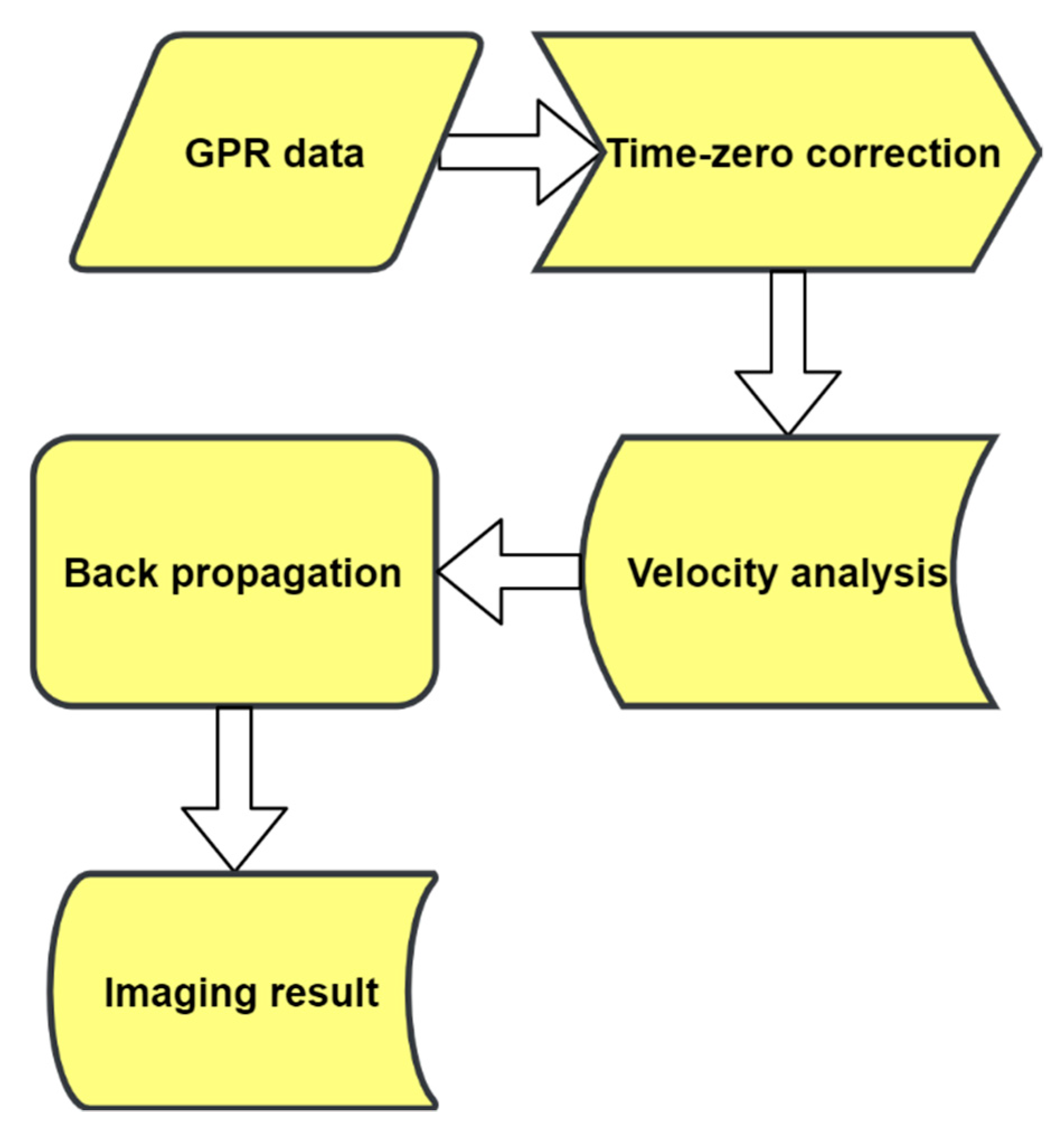
2.1.2. Workflow of RTM
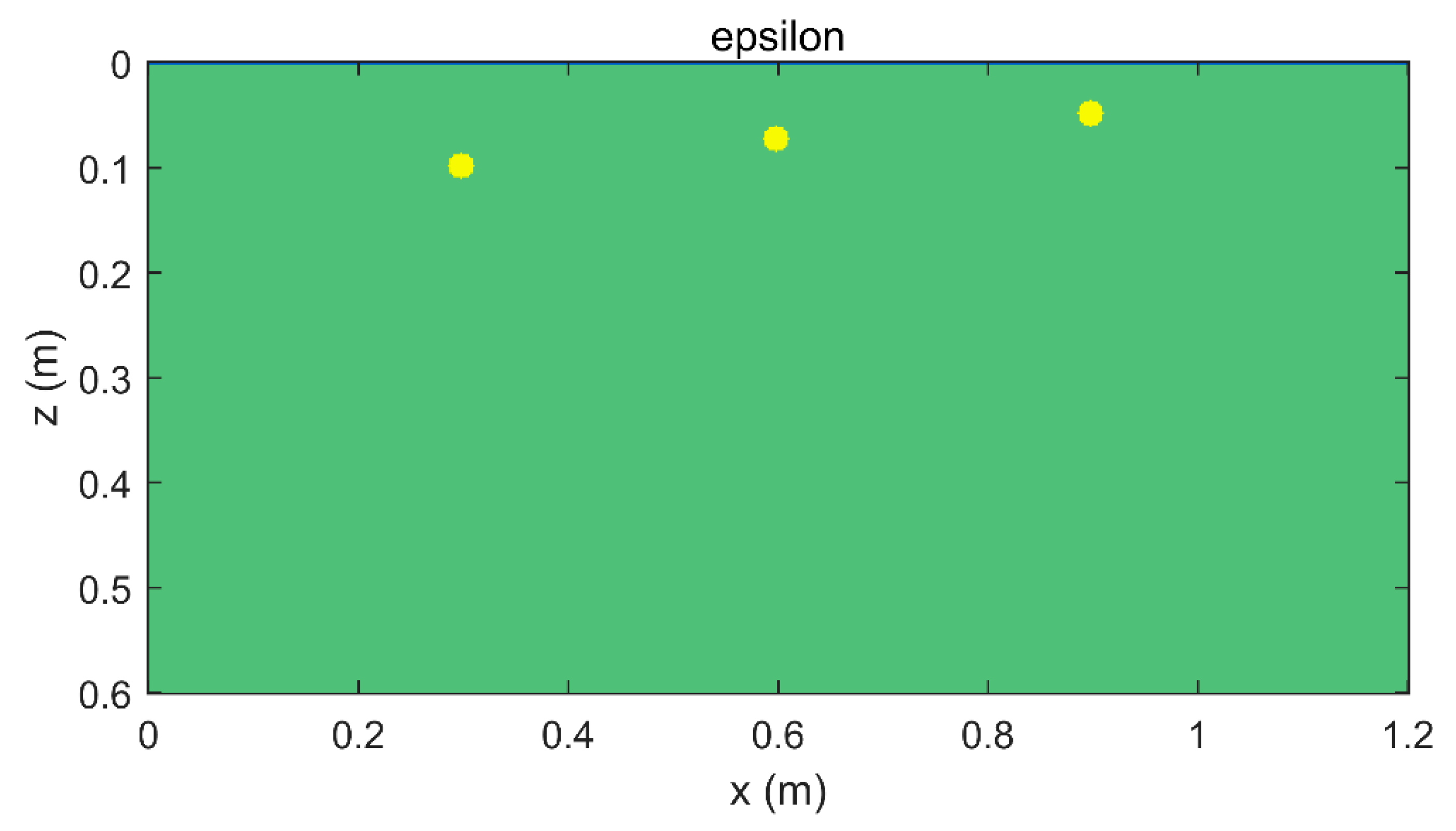
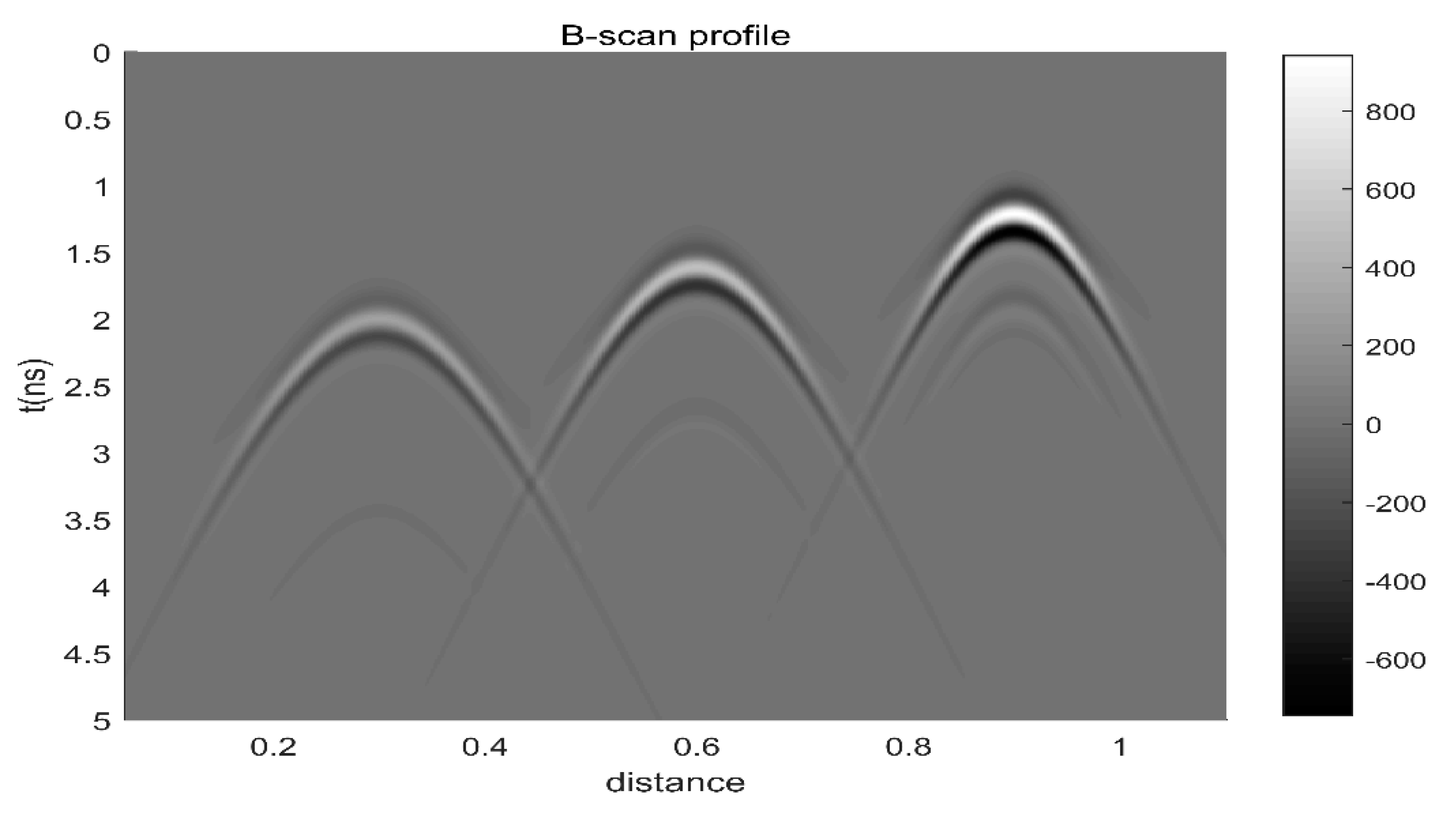
2.2. Synthetic Datasets
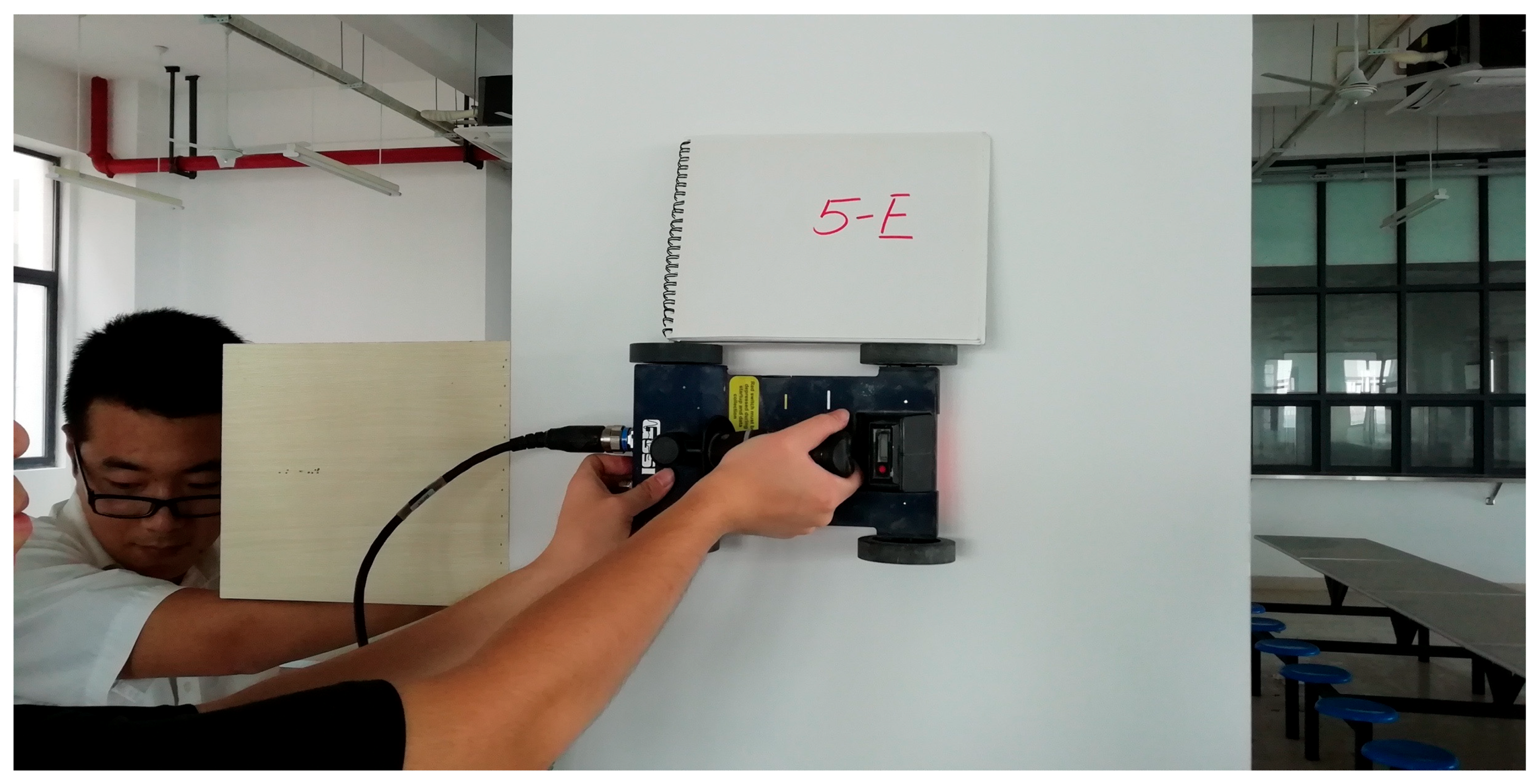
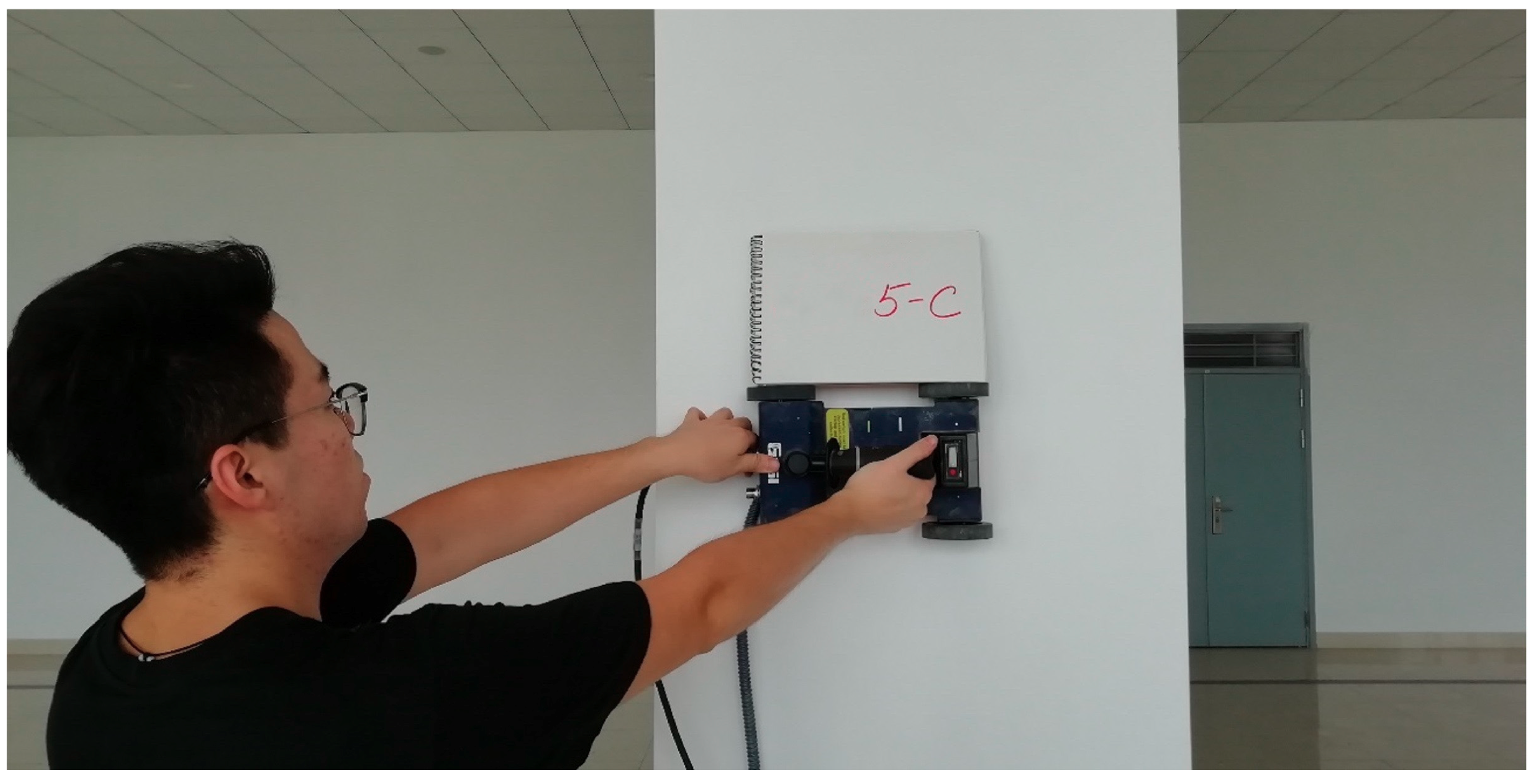
2.3. Real Case Datasets
3. Results
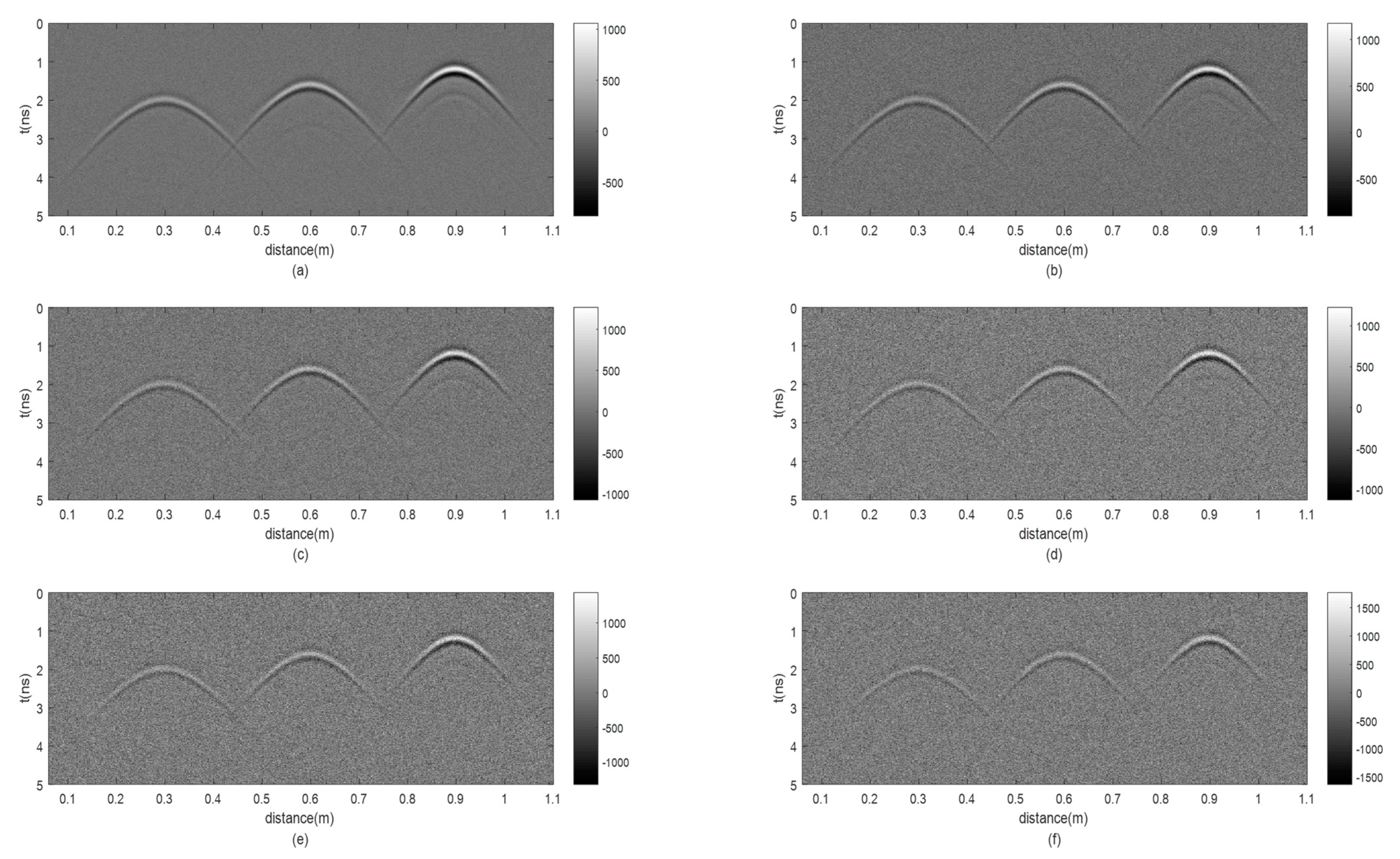
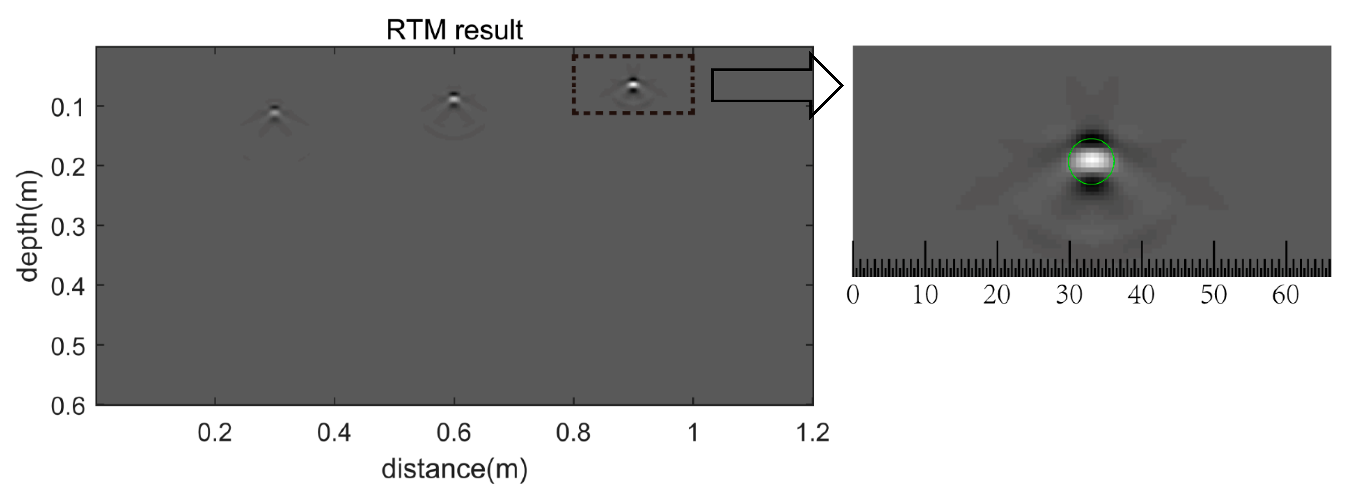
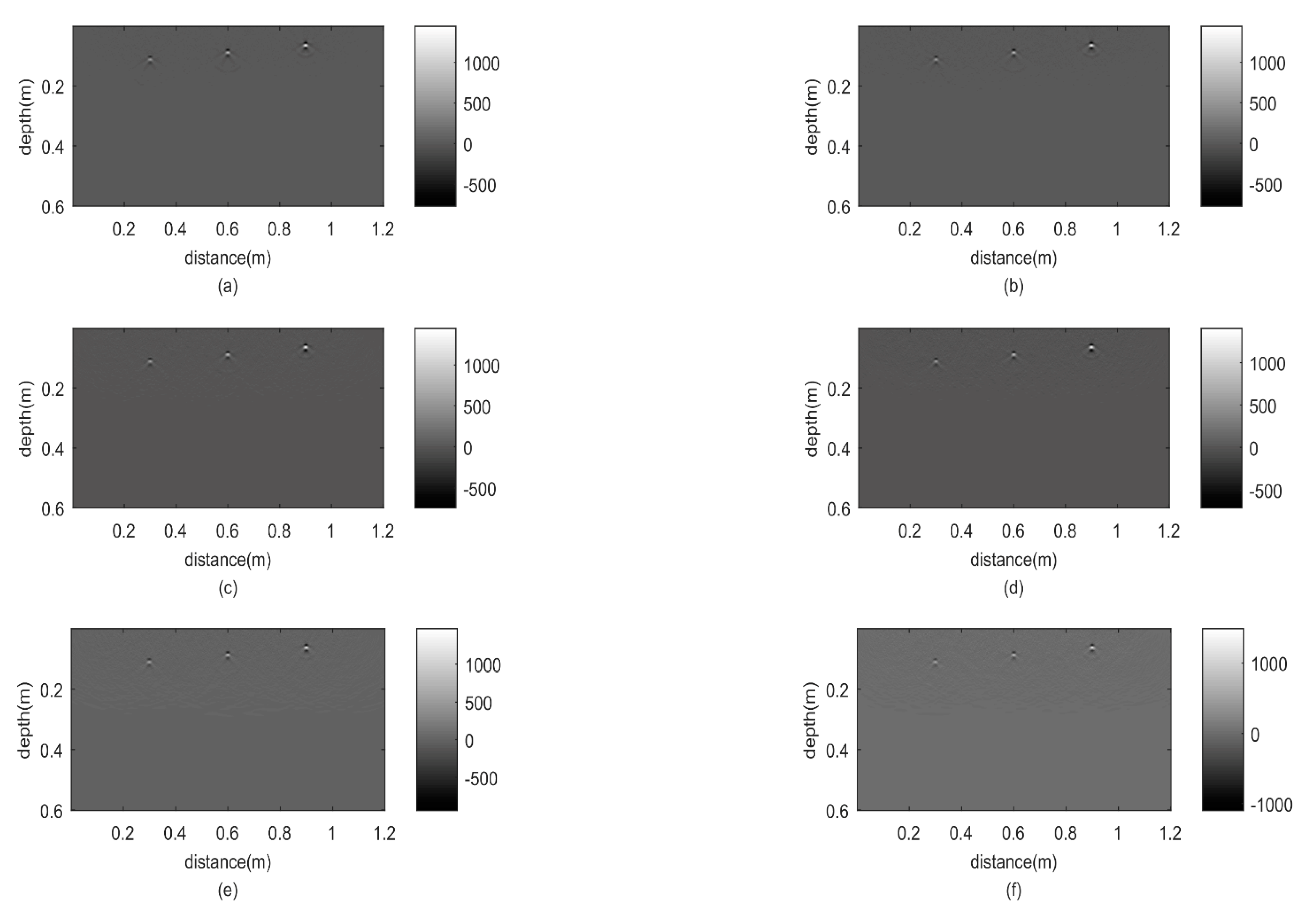
3.1. Synthetic Data Test
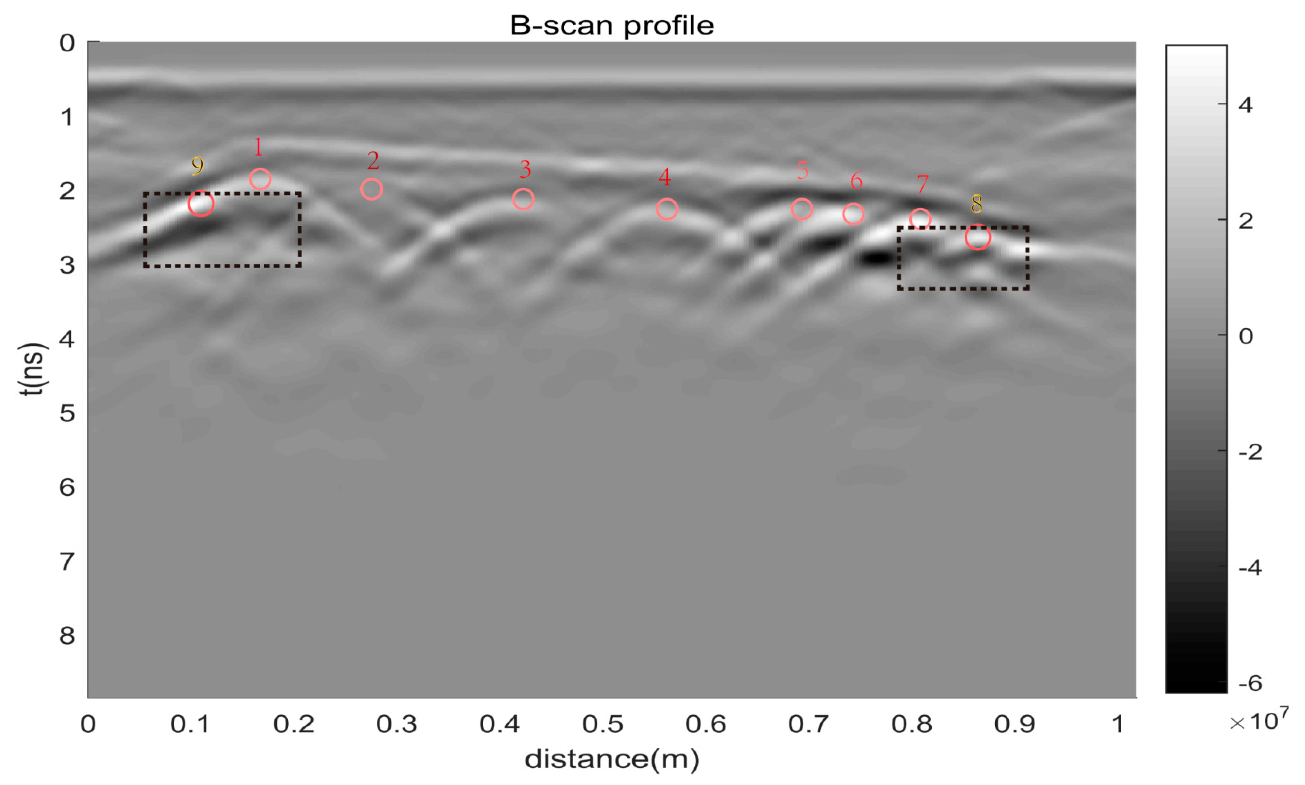
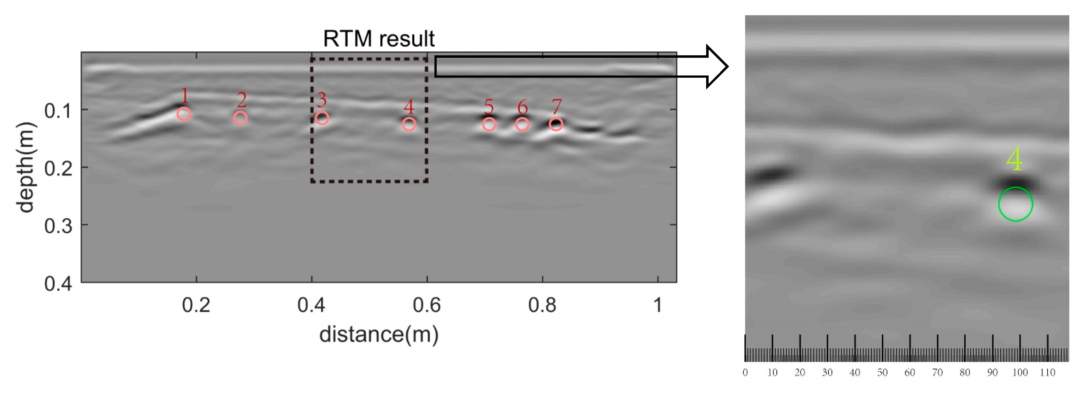
3.2. Real Field Data Test
4. Discussion
5. Conclusions
Author Contributions
Funding
Institutional Review Board Statement
Informed Consent Statement
Data Availability Statement
Conflicts of Interest
References
- Lambot, S.; Slob, E.C.; Van den Bosch, I.; Stockbroeckx, B.; Vanclooster, M. Modeling of ground-penetrating Radar for accurate characterization of subsurface electric properties. IEEE Trans. Geosci. Remote Sens. 2004, 42, 2555–2568. [Google Scholar] [CrossRef]
- Lunt, I.A.; Hubbard, S.S.; Rubin, Y. Soil moisture content estimation using ground-penetrating radar reflection data. J. Hydrol. 2005, 307, 254–269. [Google Scholar] [CrossRef]
- Loke, M.H.; Chambers, J.E.; Rucker, D.F.; Kuras, O.; Wilkinson, P.B. Recent developments in the direct-current geoelectrical imaging method. J. Appl. Geophys. 2013, 95, 135–156. [Google Scholar] [CrossRef]
- Gader, P.D.; Mystkowski, M.; Zhao, Y.X. Landmine detection with ground penetrating radar using hidden Markov models. IEEE Trans. Geosci. Remote Sens. 2001, 39, 1231–1244. [Google Scholar] [CrossRef]
- Torrione, P.A.; Morton, K.D.; Sakaguchi, R.; Collins, L.M. Histograms of Oriented Gradients for Landmine Detection in Ground-Penetrating Radar Data. IEEE Trans. Geosci. Remote Sens. 2014, 52, 1539–1550. [Google Scholar] [CrossRef]
- Wilson, J.N.; Gader, P.; Lee, W.; Frigui, H.; Ho, K.C. A Large-Scale Systematic Evaluation of Algorithms Using Ground-Penetrating Radar for Landmine Detection and Discrimination. IEEE Trans. Geosci. Remote Sens. 2007, 45, 2560–2572. [Google Scholar] [CrossRef]
- Demanet, D.; Renardy, F.; Vanneste, K.; Jongmans, D.; Camelbeeck, T.; Meghraoui, M. The use of geophysical prospecting for imaging active faults in the Roer Graben, Belgium. Geophysics 2001, 66, 78–89. [Google Scholar] [CrossRef]
- Vasco, D.W.; Peterson, J.E.; Lee, K.H. Ground-penetrating radar velocity tomography in heterogeneous and anisotropic media. Geophysics 1997, 62, 1758–1773. [Google Scholar] [CrossRef]
- Lai, J.L.; Xu, Y.; Zhang, X.P.; Xiao, L.; Yan, Q.; Meng, X.; Zhou, B.; Dong, Z.H.; Zhao, D. Comparison of dielectric properties and structure of lunar regolith at Chang’e-3 and Chang’e-4 landing sites revealed by ground-penetrating radar. Geophys. Res. Lett. 2019, 46, 12783–12793. [Google Scholar] [CrossRef]
- Zhang, L.; Zeng, Z.F.; Li, J.; Lin, J.Y.; Hu, Y.S.; Wang, X.G.; Sun, X.D. Simulation of the Lunar Regolith and Lunar-Penetrating Radar Data Processing. IEEE J. Sel. Top. Appl. Earth Obs. Remote Sens. 2018, 11, 655–663. [Google Scholar] [CrossRef]
- Grandjean, G.; Gourry, J.C.; Bitri, A. Evaluation of GPR techniques for civil-engineering applications: Study on a test site. J. Appl. Geophys. 2000, 45, 141–156. [Google Scholar] [CrossRef]
- Lai, W.W.L.; Derobert, X.; Annan, P. A review of Ground Penetrating Radar application in civil engineering: A 30-year journey from Locating and Testing to Imaging and Diagnosis. NDT E Int. 2018, 96, 58–78. [Google Scholar] [CrossRef]
- Hugenschmidt, J. Concrete bridge inspection with a mobile GPR system. Constr. Build. Mater. 2002, 16, 147–154. [Google Scholar] [CrossRef]
- Leucci, G. Ground Penetrating Radar: An Application to Estimate Volumetric Water Content and Reinforced Bar Diameter in Concrete Structures. J. Adv. Concr. Technol. 2012, 10, 411–422. [Google Scholar] [CrossRef] [Green Version]
- Tosti, F.; Ferrante, C. Using Ground Penetrating Radar Methods to Investigate Reinforced Concrete Structures. Surv. Geophys. 2020, 41, 485–530. [Google Scholar] [CrossRef]
- Zhou, F.; Chen, Z.C.; Liu, H.; Cui, J.; Spencer, B.E.; Fang, G.Y. Simultaneous Estimation of Rebar Diameter and Cover Thickness by a GPR-EMI Dual Sensor. Sensors 2018, 18, 2969. [Google Scholar] [CrossRef] [PubMed] [Green Version]
- Chang, C.W.; Lin, C.H.; Lien, H.S. Measurement radius of reinforcing steel bar in concrete using digital image GPR. Constr. Build. Mater. 2009, 23, 1057–1063. [Google Scholar] [CrossRef]
- Shaw, M.R.; Molyneaux, T.C.K.; Millard, S.G.; Taylor, M.J.; Bungey, J.H. Assessing bar size of steel reinforcement in concrete using ground penetrating radar and neural networks. Insight Non Destruct. Test. Cond. Monit. 2003, 45, 813–816. [Google Scholar] [CrossRef]
- Tesic, K.; Baricevic, A.; Serdar, M. Non-Destructive Corrosion Inspection of Reinforced Concrete Using Ground-Penetrating Radar: A Review. Materials 2021, 14, 975. [Google Scholar] [CrossRef] [PubMed]
- Tarussov, A.; Vandry, M.; De La Haza, A. Condition assessment of concrete structures using a new analysis method: Ground-penetrating radar computer-assisted visual interpretation. Constr. Build. Mater. 2013, 38, 1246–1254. [Google Scholar] [CrossRef]
- Liu, H.; Lin, C.X.; Cui, J.; Fan, L.S.; Xie, X.Y.; Spencer, B.F. Detection and localization of rebar in concrete by deep learning using ground penetrating radar. Autom. Constr. 2020, 118, 103279. [Google Scholar] [CrossRef]
- Giannakis, I.; Giannopoulos, A.; Warren, C. A Machine Learning Scheme for Estimating the Diameter of Reinforcing Bars Using Ground Penetrating Radar. IEEE Geosci. Remote Sens. Lett. 2021, 18, 461–465. [Google Scholar] [CrossRef] [Green Version]
- Zadhouse, H.; Giannopoulos, A.; Giannakis, I. Optimising the Complex Refractive Index Model for Estimating the Permittivity of Heterogeneous Concrete Models. Remote Sens. 2021, 13, 723. [Google Scholar] [CrossRef]
- Kalogeropoulos, A.; Van der Kruk, J.; Hugenschmidt, J.; Bikowski, J.; Bruhwiler, E. Full-waveform GPR inversion to assess chloride gradients in concrete. NDT E Int. 2013, 57, 74–84. [Google Scholar] [CrossRef]
- Alani, A.M.; Giannakis, I.; Zou, L.L.; Lantini, L.; Tosti, F. Reverse-time migration for evaluating the internal structure of tree-trunks using ground-penetrating radar. NDT E Int. 2020, 115, 102294. [Google Scholar] [CrossRef]
- Ozdemir, C.; Demirci, S.; Yigit, E.; Yilmaz, B. A Review on Migration Methods in B-Scan Ground Penetrating Radar Imaging. Math. Probl. Eng. 2014, 2014, 280738. [Google Scholar] [CrossRef] [Green Version]
- Bitri, A.; Grandjean, G. Frequency–wavenumber modelling and migration of 2D GPR data in moderately heterogeneous dispersive Media. Geophys. Prospect. 1998, 46, 287–301. [Google Scholar] [CrossRef]
- Moran, M.L.; Greenfield, R.J.; Arcone, S.A.; Delaney, A.J. Multidimensional GPR array processing using Kirchhoff migration. J. Appl. Geophys. 2000, 43, 281–295. [Google Scholar] [CrossRef]
- Bradford, J.H. Reverse-time prestack depth migration of GPR data from topography for amplitude reconstruction in complex environments. J. Earth Sci. 2015, 26, 791–798. [Google Scholar] [CrossRef]
- Fisher, E.; Mcmechan, G.A.; Annan, A.P.; Cosway, S.W. Examples of reverse-time migration of single-channel, ground-penetrating radar profiles. Geophysics 1992, 57, 577–586. [Google Scholar] [CrossRef]
- Zhou, H.; Sato, M.; Liu, H.J. Migration velocity analysis and prestack migration of common-transmitter GPR data. IEEE Trans. Geosci. Remote Sens. 2005, 43, 86–91. [Google Scholar] [CrossRef]
- Liu, S.X.; Lei, L.L.; Fu, L.; Wu, J.J. Application of pre-stack reverse time migration based on FWI velocity estimation to ground penetrating radar data. J. Appl. Geophys. 2014, 107, 1–7. [Google Scholar] [CrossRef]
- Liu, H.; Long, Z.J.; Han, F.; Fang, G.Y.; Liu, Q.H. Frequency-Domain Reverse-Time Migration of Ground Penetrating Radar Based on Layered Medium Green’s Functions. IEEE J. Sel. Top. Appl. Earth Obs. Remote Sens. 2018, 11, 2957–2965. [Google Scholar] [CrossRef]
- Huo, J.J.; Zhao, Q.; Zhao, B.Z.; Liu, L.B.; Ma, C.G.; Guo, J.Y.; Xie, L.H. Energy Flow Domain Reverse-Time Migration for Borehole Radar. IEEE Trans. Geosci. Remote Sens. 2019, 57, 7221–7231. [Google Scholar] [CrossRef]
- Irving, J.; Knight, R. Numerical modeling of ground-penetrating radar in 2-D using MATLAB. Comput. Geosci. 2006, 32, 1247–1258. [Google Scholar] [CrossRef]


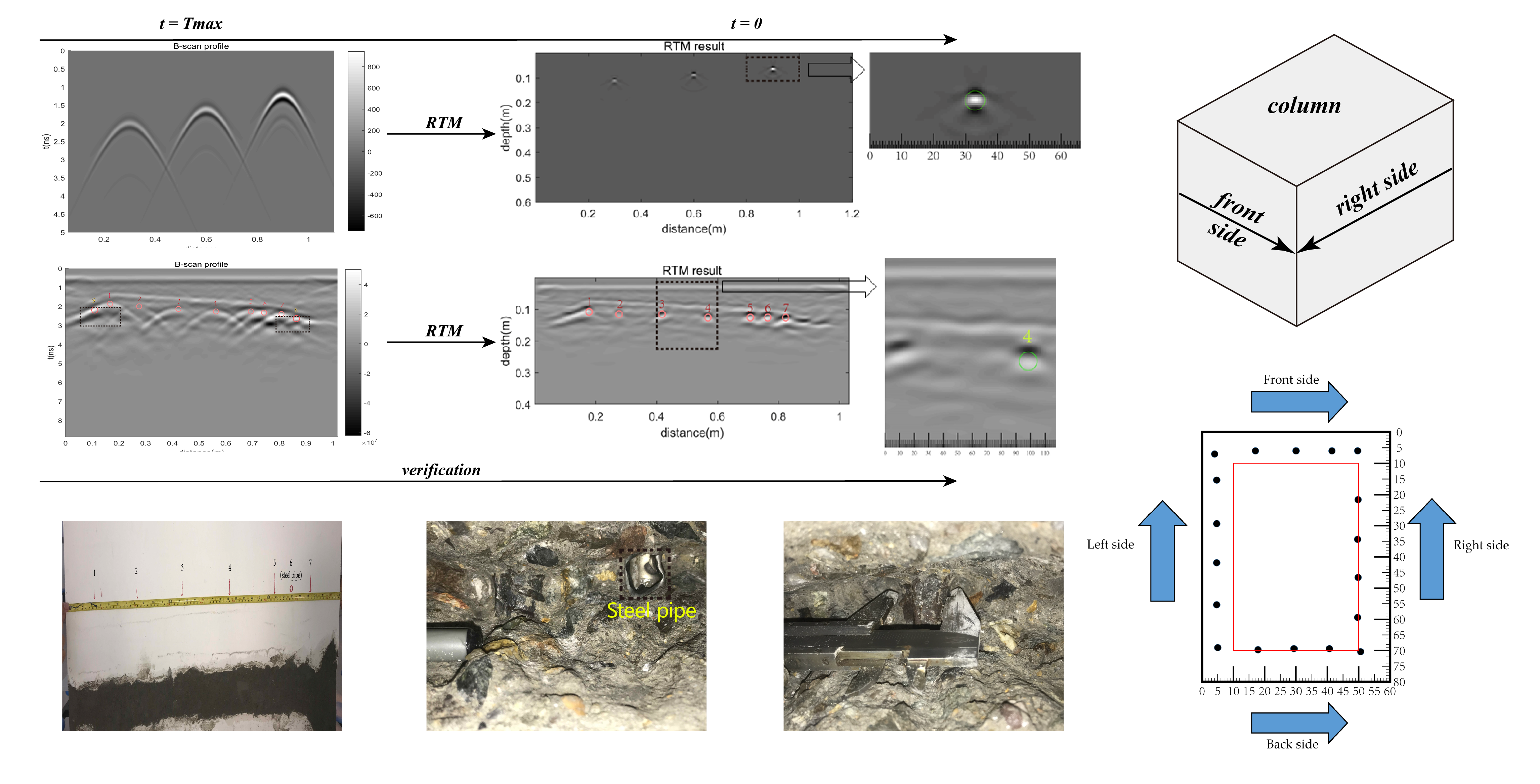
| Hyperbola | Position | Feature |
|---|---|---|
| 1 | (0.17 m, 1.9 ns) | Normal 1 |
| 2 | (0.24 m, 2 ns) | Normal but weak |
| 3 | (0.42 m, 2.1 ns) | Normal 1 |
| 4 | (0.56 m, 2.2 ns) | Normal 1 |
| 5 | (0.7 m, 2.2 ns) | Overlapped |
| 6 | (0.74 m, 2.25 ns) | Overlapped |
| 7 | (0.81 m, 2.3 ns) | Overlapped |
| 8 (in doubt) | (0.86 m, 2.6 ns) | Incomplete and small |
| 9 (in doubt) | (0.11 m, 2.15 ns) | Overlapped and weak |
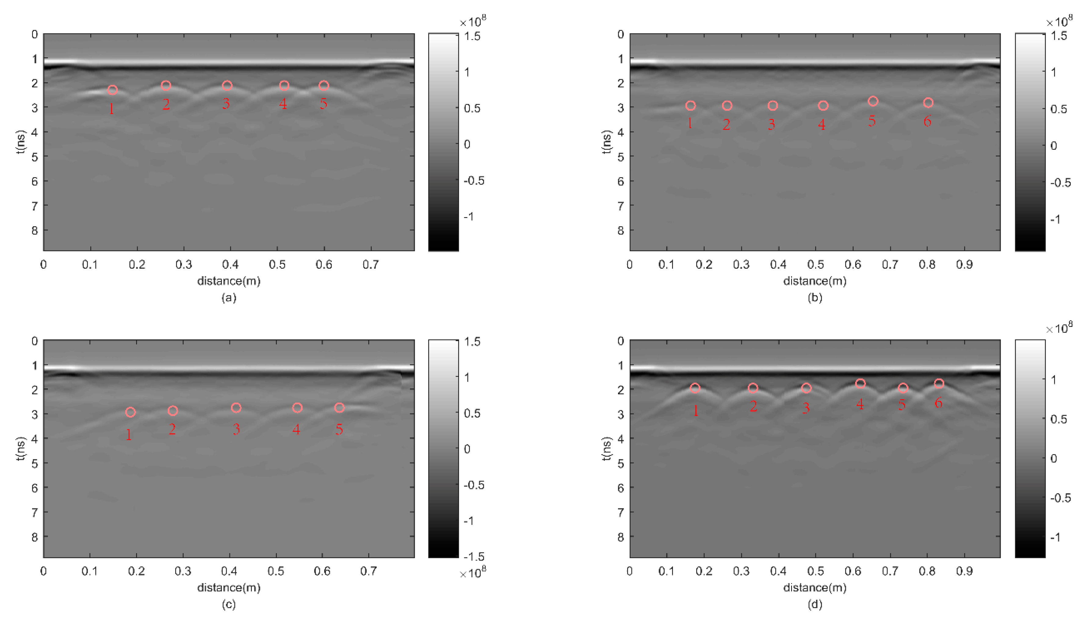
| B-Scan Profile | Hyperbola | Position | Feature |
|---|---|---|---|
| Front-side | 1 | (0.14 m, 2.4 ns) | Normal 1 |
| 2 | (0.26 m, 2.3 ns) | Normal 1 | |
| 3 | (0.38 m, 2.3 ns) | Normal 1 | |
| 4 | (0.52 m, 2.3 ns) | Normal 1 | |
| 5 | (0.6 m, 2.3 ns) | Normal 1 | |
| Right-side | 1 | (0.16 m, 3 ns) | Straight |
| 2 | (0.25 m, 3 ns) | Normal 1 | |
| 3 | (0.38 m, 3 ns) | Normal 1 | |
| 4 | (0.52 m, 3 ns) | Normal 1 | |
| 5 | (0.65 m, 2.9 ns) | Normal 1 | |
| 6 | (0.8 m, 2.95 ns) | Normal 1 | |
| Back-side | 1 | (0.19 m, 3 ns) | Normal 1 |
| 2 | (0.28 m, 3 ns) | Normal 1 | |
| 3 | (0.41 m, 2.9 ns) | Normal 1 | |
| 4 | (0.54 m, 2.9 ns) | Normal 1 | |
| 5 | (0.65 m, 2.9 ns) | Straight | |
| Left-side | 1 | (0.18 m, 2 ns) | Normal 1 |
| 2 | (0.33 m, 2 ns) | Normal 1 | |
| 3 | (0.48 m, 2 ns) | Normal 1 | |
| 4 | (0.62 m, 2 ns) | Normal 1 | |
| 5 | (0.73 m, 2 ns) | Normal 1 | |
| 6 | (0.84 m, 2 ns) | Normal 1 |
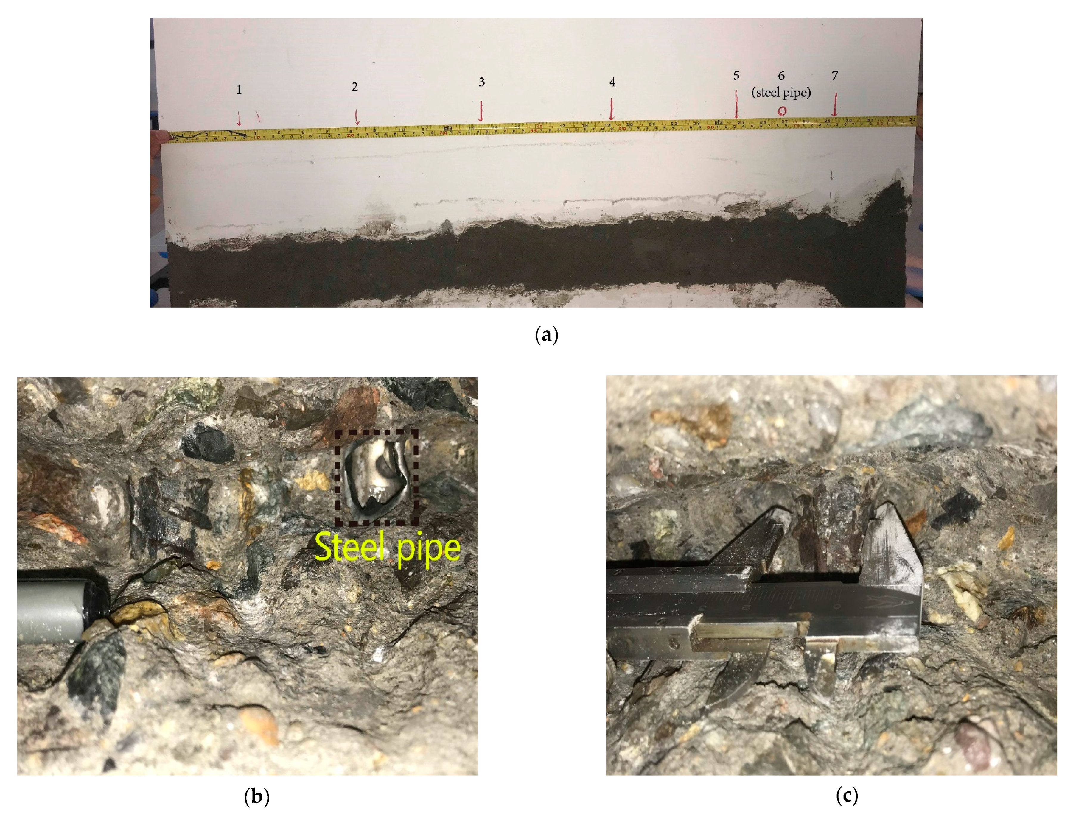
| Rebar | Position | Feature |
|---|---|---|
| 1 | (0.16 m, 0.11 m) | Striped |
| 2 | (0.28 m, 0.12 m) | Dotted and weak |
| 3 | (0.42 m, 0.12 m) | Dotted |
| 4 | (0.56 m, 0.13 m) | Dotted |
| 5 | (0.7 m, 0.13 m) | Dotted |
| 6 | (0.75 m, 0.13 m) | Dotted |
| 7 | (0.81 m, 0.13 m) | Striped |
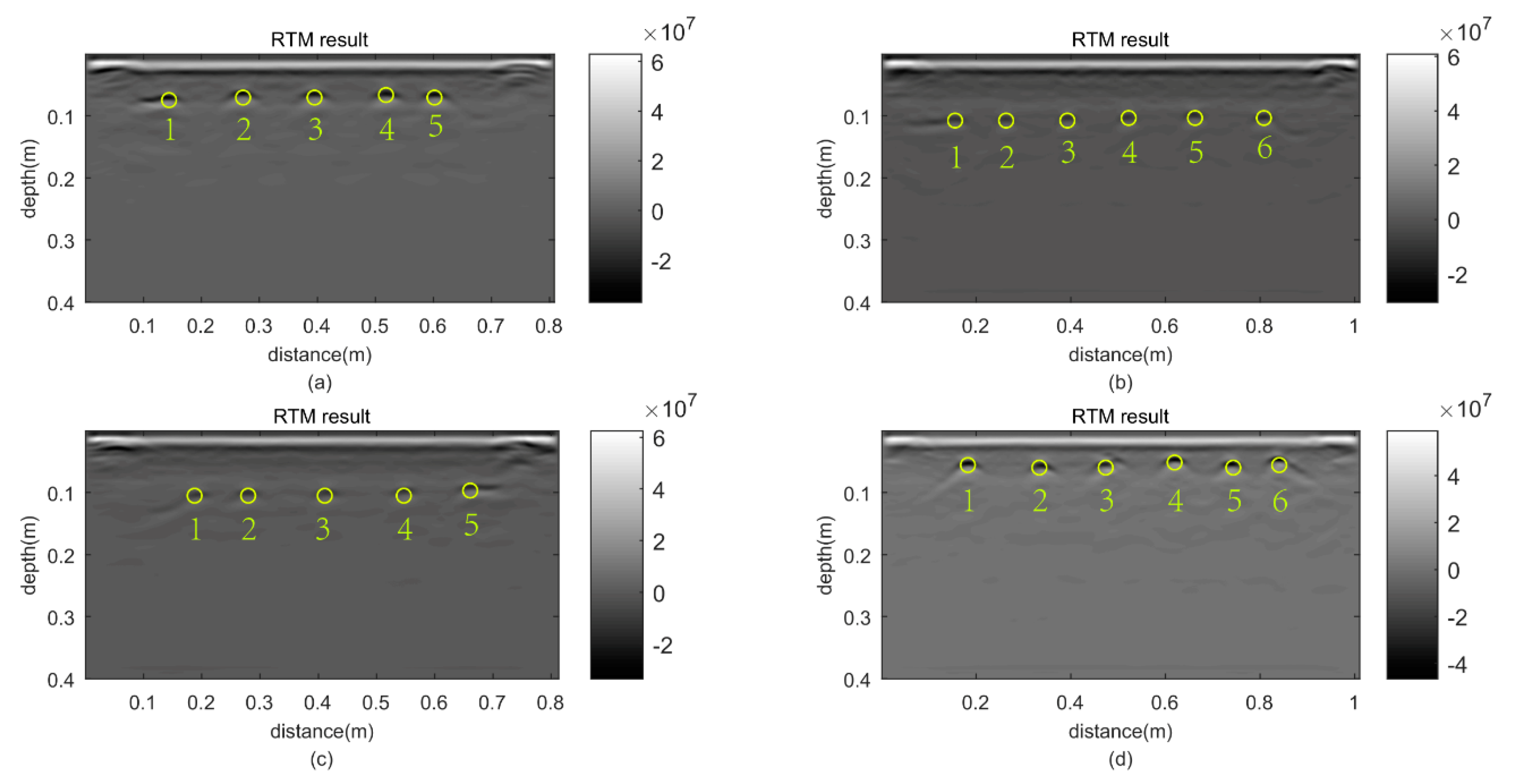
| Migration Image | Rebar | Position | Feature |
|---|---|---|---|
| Front-side | 1 | (0.14 m, 0.07 m) | Striped |
| 2 | (0.27 m, 0.06 m) | Curved | |
| 3 | (0.4 m, 0.06 m) | Curved | |
| 4 | (0.52 m, 0.06 m) | Curved | |
| 5 | (0.6 m, 0.06 m) | Curved | |
| Right-side | 1 | (0.15 m, 0.11 m) | Striped |
| 2 | (0.25 m, 0.11 m) | Dotted | |
| 3 | (0.4 m, 0.11 m) | Dotted | |
| 4 | (0.52 m, 0.11 m) | Dotted | |
| 5 | (0.65 m, 0.1 m) | Dotted | |
| 6 | (0.82 m, 0.11 m) | Dotted | |
| Back-side | 1 | (0.2 m, 0.11 m) | (Dotted with a concave downward tail) |
| 2 | (0.28 m, 0.11 m) | Dotted | |
| 3 | (0.41 m, 0.11 m) | Dotted | |
| 4 | (0.55 m, 0.1 m) | Dotted | |
| 5 | (0.65 m, 0.1 m) | Striped | |
| Left-side | 1 | (0.18 m, 0.05 m) | (Curved with a downward tail) |
| 2 | (0.33 m, 0.05 m) | Curved | |
| 3 | (0.47 m, 0.05 m) | Curved | |
| 4 | (0.61 m, 0.04 m) | Curved | |
| 5 | (0.75 m, 0.06 m) | Curved | |
| 6 | (0.84 m, 0.05 m) | (Curved with a downward tail) |
Publisher’s Note: MDPI stays neutral with regard to jurisdictional claims in published maps and institutional affiliations. |
© 2021 by the authors. Licensee MDPI, Basel, Switzerland. This article is an open access article distributed under the terms and conditions of the Creative Commons Attribution (CC BY) license (https://creativecommons.org/licenses/by/4.0/).
Share and Cite
Shen, R.; Zhao, Y.; Hu, S.; Li, B.; Bi, W. Reverse-Time Migration Imaging of Ground-Penetrating Radar in NDT of Reinforced Concrete Structures. Remote Sens. 2021, 13, 2020. https://doi.org/10.3390/rs13102020
Shen R, Zhao Y, Hu S, Li B, Bi W. Reverse-Time Migration Imaging of Ground-Penetrating Radar in NDT of Reinforced Concrete Structures. Remote Sensing. 2021; 13(10):2020. https://doi.org/10.3390/rs13102020
Chicago/Turabian StyleShen, Ruiqing, Yonghui Zhao, Shufan Hu, Bo Li, and Wenda Bi. 2021. "Reverse-Time Migration Imaging of Ground-Penetrating Radar in NDT of Reinforced Concrete Structures" Remote Sensing 13, no. 10: 2020. https://doi.org/10.3390/rs13102020
APA StyleShen, R., Zhao, Y., Hu, S., Li, B., & Bi, W. (2021). Reverse-Time Migration Imaging of Ground-Penetrating Radar in NDT of Reinforced Concrete Structures. Remote Sensing, 13(10), 2020. https://doi.org/10.3390/rs13102020