Abstract
The evaluation and inspection of steel bars in reinforced concrete structures are critical for prolonging the service life of buildings. In this regard, ground-penetrating radar (GPR) has been a crucial alternative due to its non-invasiveness and convenience. This paper reports the experimental activities on a test-site area inside a camp in Shanghai, China. To assess the concrete structures of the building, GPR was employed for the detection and localization of rebars in columns, beams, and floors. From the GPR B-scan profiles acquired using a high-frequency antenna, the exact quantity of reinforcements was identified according to the hyperbola responses. Considering the difficulty of inferring the exact position and the scale of the rebars, we applied reverse time migration (RTM) to collapse the hyperbolic response and retrieve the target in a migrated image. To verify the effectiveness of the RTM algorithm, we carried out an experiment on a concrete model with three reinforced bars. We also utilized the RTM algorithm to process the B-scan profiles collected in a column that was later excavated. The imaging results validated the capacity of RTM in localizing and shaping rebars. Then, we employed the RTM algorithm for the GPR B-scan data collected from the other column. Based on the imaging profile, the quantity and positions of the rebars were correctly determined. Moreover, the thickness of the protective layer was evaluated according to the migrated result. These results demonstrate that GPR combined with RTM could provide useful foundation data for structural evaluation.
1. Introduction
Ground-penetrating radar (GPR) has been a high-efficiency near-surface geophysical method widely applied in many application fields, such as hydrological monitoring [1,2,3], landmine detection [4,5,6], geological exploration [7,8], lunar exploration [9,10] and civil engineering [11,12]. As an effective tool in non-destructive testing (NDT), GPR is commonly adopted to evaluate concrete structures and detect reinforcements in civil engineering [13,14]. Specifically, the main applications of GPR in reinforced concrete materials and structures are [15]: (1) the location of reinforcing bars; (2) the detection of rebar corrosion; (3) the estimation of the rebar size; (4) the evaluation of the concrete cover; (5) the structural detailing of anchorages and joints in major structures/infrastructures; (6) the assessment of concrete characteristics by analyzing the material dielectric properties.
Zhou et al. [16] used GPR in combination with the electromagnetic induction (EMI) method to accurately locate reinforcing bars. Chang et al. [17] reported a physical model based on the use of digital image GPR for measuring the radius of reinforcing steel bars in concrete. Shaw et al. [18] developed a neural network approach to automate the estimation of the rebar size diameter from data collected with the transducer axis parallel and orthogonal to the bar orientation. Tesic et al. summarized corrosion inspection of reinforced concrete using GPR over the past two decades [19]. Tarussov et al. adopted computer-assisted visual interpretation to eliminate the anomalies unrelated to structural defects and filter out random noise [20]. For detection and localization of reinforced bars, Liu et al. [21] and Giannakis et al. [22] utilized machine-learning methods to estimate the diameter of reinforcements. Moreover, the evaluation of concrete parameters is an essential research subject. Zadhoush et al. [23] optimized the Complex Refractive Index Model (CRIM) to estimate the permittivity of heterogeneous mixtures. Kalogeropoulos et al. used full-waveform inversion (FWI) to assess chloride gradients in concrete [24].
However, the raw GPR B-scan profile is not sufficient for detection and localization of steel bars. As an effective strategy of obtaining accurate underground structure, migration has been a prevalent method [25]. Currently, three of the most popular migration methods are frequency-wavenumber (F-K) migration, Kirchhoff migration, and reverse-time migration, respectively. Ozdemir et al. [26] reviewed some popular migration methods of B-scan GPR imaging, including F-K migration, Kirchhoff migration, and phase-shifted migration. Since the ability of the frequency-wavenumber domain migration relies on the given velocity model, an apparent illusion will appear in the migration results if the velocity model has low accuracy [27]. For the Kirchhoff migration, it is difficult to deal with the situation when lateral variations are presented [28]. On the other hand, reverse-time migration has few drawbacks since it is based on a two-way wave equation [29].
According to different data acquisitions, GPR reverse time migration is divided into common-offset migration and multi-offset migration. In 1992, Fisher et al. first carried out reverse time migration for common-offset GPR data [30]. Zhou et al. [31] applied a velocity analysis method based on a genetic algorithm (GA) before migration to obtain the distribution of dielectric constants. Liu et al. applied FWI to estimate subsurface velocity structure, which was later used in RTM [32]. To solve the problem of multi-offset GPR reverse time migration in rugged terrain, Bradford proposed a reverse time migration algorithm considering electromagnetic wave amplitude compensation and applied it to synthetic and measured GPR data processing [29]. Liu et al. proposed a frequency-domain reverse-time migration (RTM) algorithm based on the layered medium dyadic Green’s function (DGF) and applied the algorithm to image potential larva rocks under the lunar surface [33]. Huo et al. [34] proposed an energy-flow domain reverse time migration, which inherits the advantages of traditional RTM and improves the lateral resolution and the ability to characterize the anomaly boundary.
In this paper, we apply the RTM method to process the synthetic datasets and the real field datasets for retrieving the shape and localizing positions of rebars. To validate the effectiveness of the RTM algorithm, we cut a column. Based on the verified result, we process the datasets of the other column.
2. Materials and Methods
2.1. Reverse-Time Migration
2.1.1. Theory
In 2D situation, the propagation of the TM mode electromagnetic wave follows the equations as:
where Hx and Hy represent the magnetic field in the X and Y directions, respectively; Ez is the electric field in the Z direction; is the conductivity, is the equivalent specific reluctance; is the dielectric constant; is the magnetic conductivity.
The solution of Equations (1)–(3) is usually obtained by the finite-difference-time-domain (FDTD) method, which can be expressed as:
where
Assuming that the travel-times of reflections are twice that of the reflector-to-receiver times, the energy of reflections received by receivers can back-propagate to locations of reflectors with half the real velocity. The expression of the inverse time extrapolation formula of the electromagnetic field is as follows:
where
The wavefield is propagated through Equations (8)–(10) from the maximum time to time = 0. The wavefield at time = 0 is the migrated wavefield, that is:
where I and E denote wave fields at zero time and between zero time and the maximum, respectively.
2.1.2. Workflow of RTM
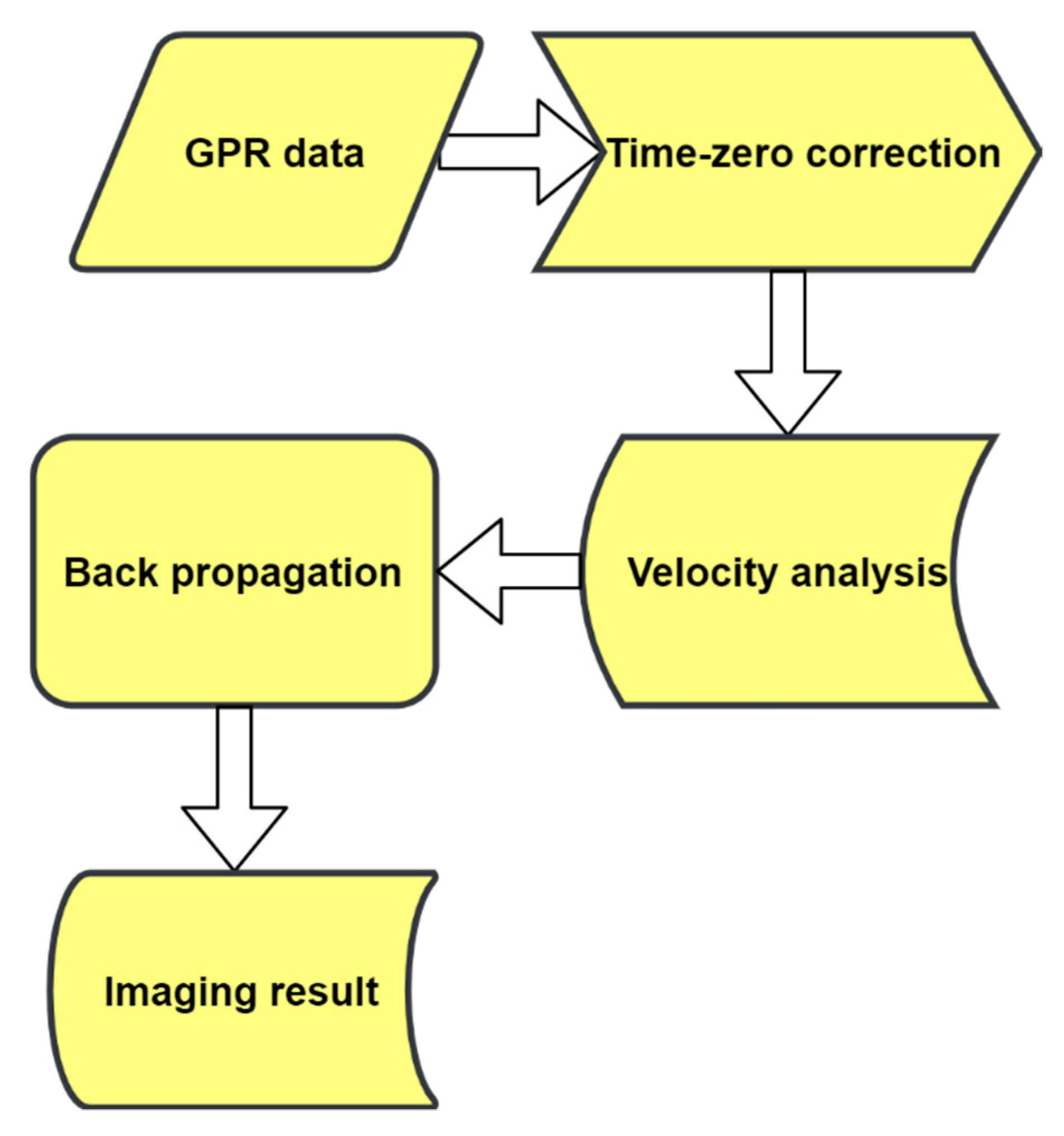
The flowchart of RTM is shown in Figure 1.

Figure 1.
Flowchart of RTM for rebar detection and localization.
First, a time-zero correction is applied to the recorded GPR data. After that, the migration velocity is estimated based on prior knowledge or hyperbola fitting. The migration velocity is an essential parameter, which affects the focusing result of hyperbolas. Here, we adopt the iterative velocity estimation method, i.e., an estimation method by a trial-and-error process, to determine the migrated velocity [21,30]. Then, the recorded data is inserted at each receiver position as boundary conditions for constant-time iteration. With this extrapolation, all energy converges back to the positions of the reflectors. Finally, we obtain the migrated result to estimate the depths and diameters of the reinforced steel bars.
2.2. Synthetic Datasets
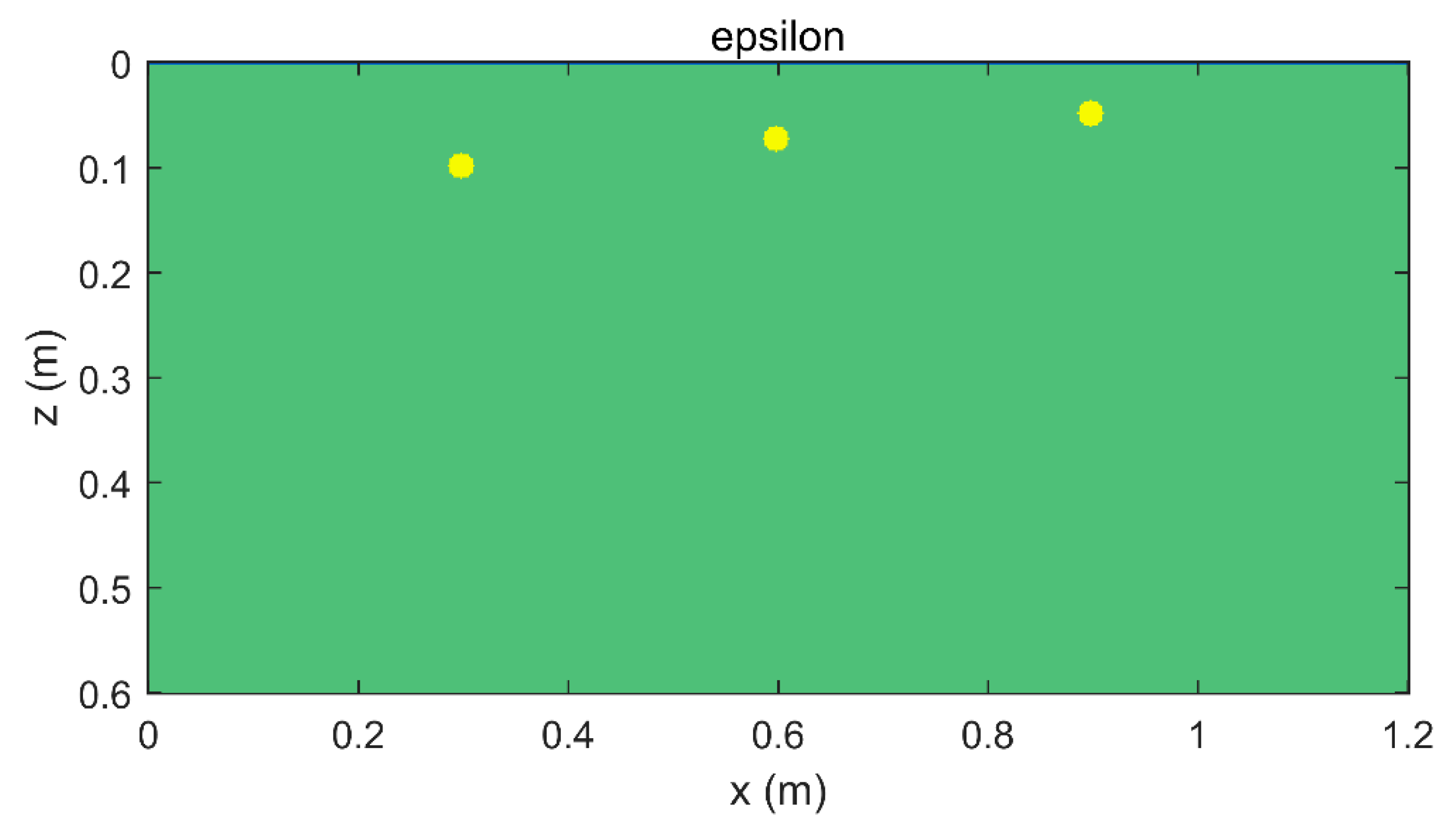
A synthetic data test is carried out to validate the ability of RTM in detecting and localizing reinforcements in concrete. Figure 2 shows the dielectric constant of reinforcement and concrete model, which is discretized into 600 × 300 grids with a grid size of 1.2 m × 0.6 m. The model contains three reinforced steel bars, which are respectively located at (0.3 m, 0.1 m), (0.6 m, 0.075 m), (0.9 m, 0.05 m). The diameter of each reinforced steel bar is 24 mm which is based on factual circumstance consideration. The relative dielectric constant of the concrete material is 6.

Figure 2.
Permittivity model.
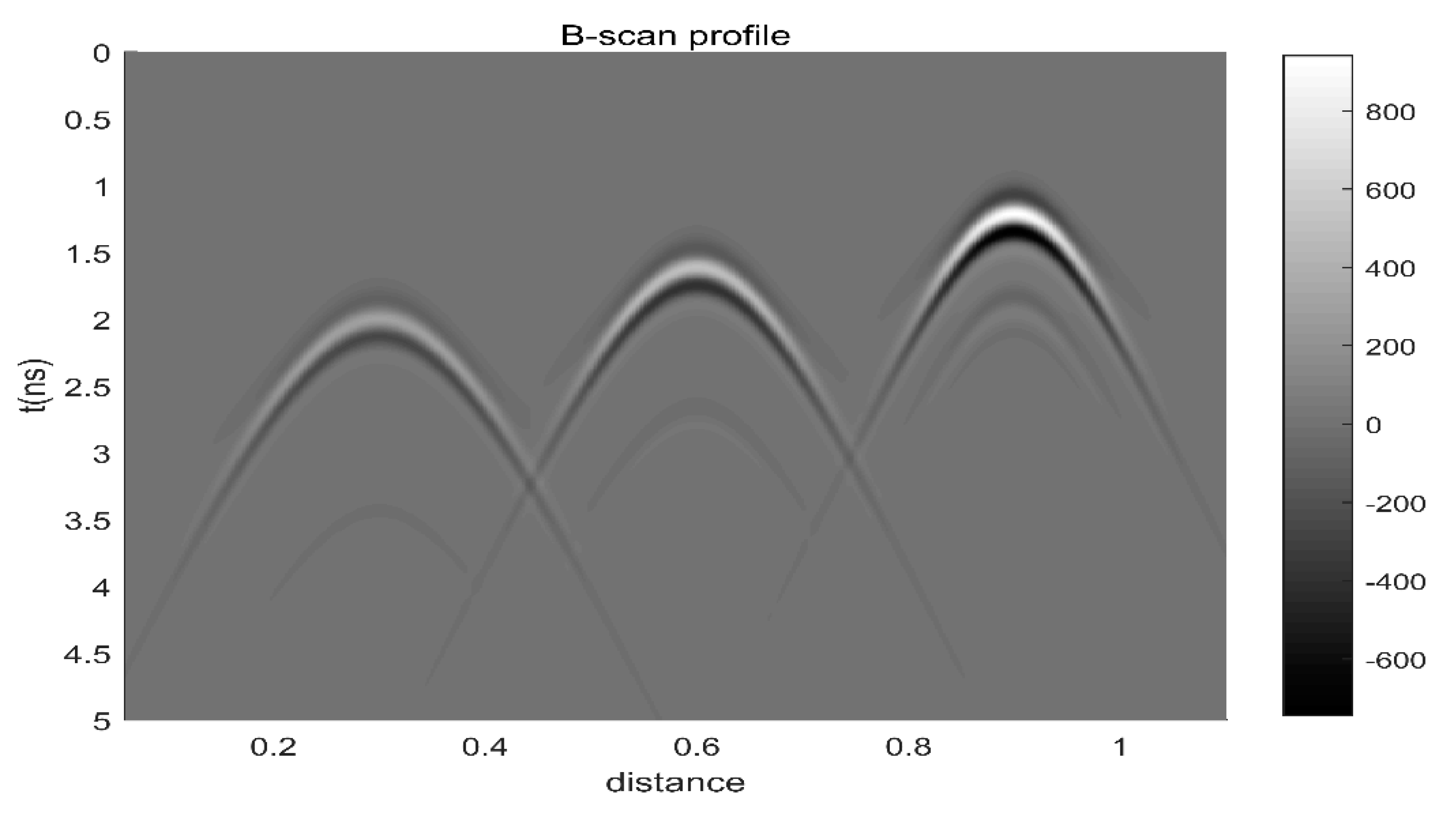
We used an FDTD algorithm [35] to model the propagation of the electromagnetic wave. The offset between the transmitter and receiver is 0.04 m, and the location of the first excitation is at (0.04 m, 0 m). A Ricker wavelet with a center frequency of 2.6 GHz is used for the source excitation. The time window is 5 ns and the number of sampling points in each trace is 1061. A total of 521 times of excitations is conducted, and the horizontal step is 2 mm. In this way, a GPR B-scan profile with 521 traces is simulated. Figure 3 shows the simulated B-scan profile, in which the direct wave has been muted and the unit is V/m. From this profile, three hyperbolas with different widths and depths are identified.

Figure 3.
B-scan profile of the synthetic data.
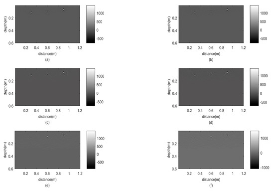
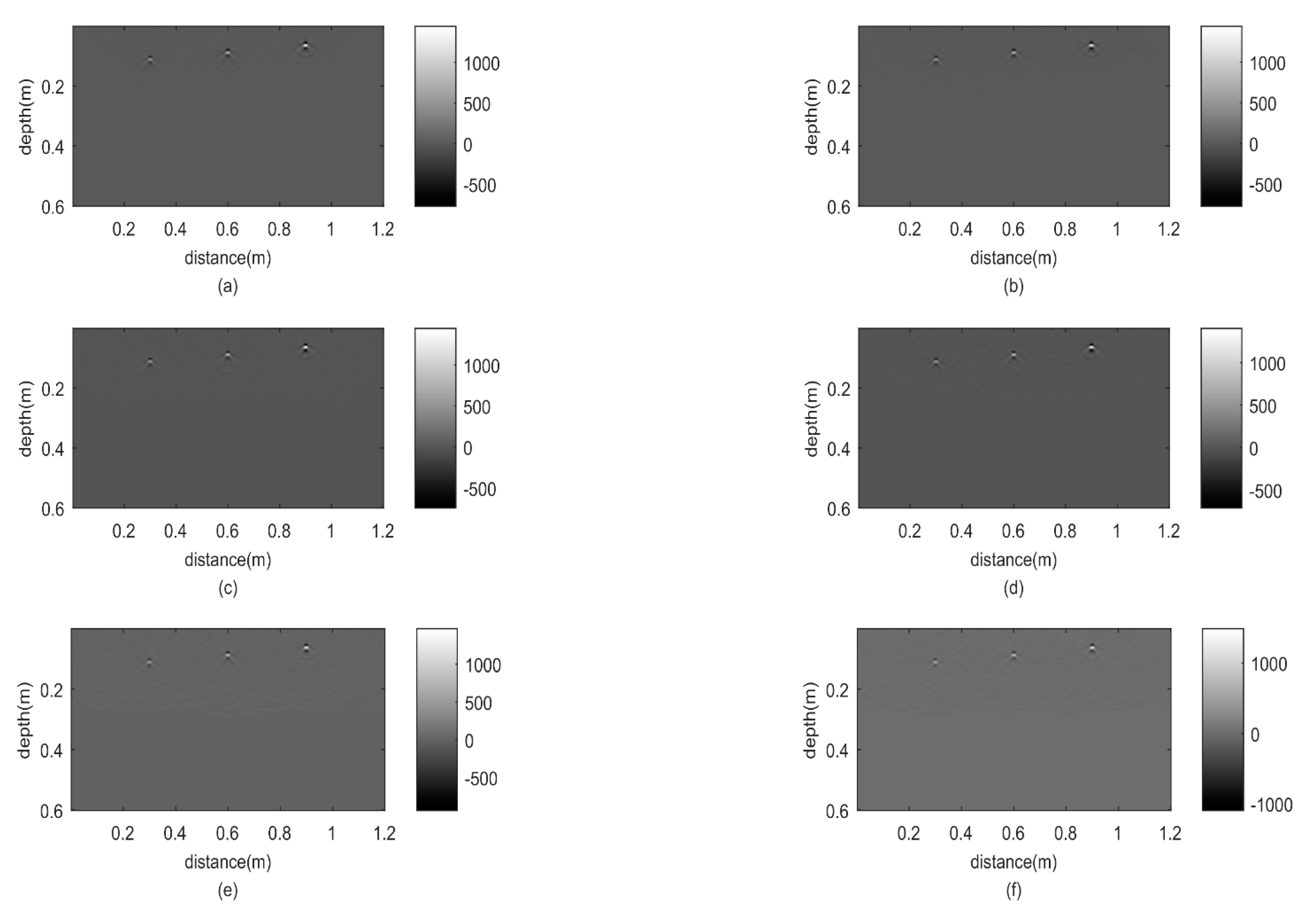
To test the ability of the RTM algorithm for noisy data, we added random noise with a value of 5–30% (with an increment of 5% each time) of the maximum amplitude in the simulated signal to the synthetic data. The B-scan with added noise at a different level is shown in Figure 4. From Figure 4a, the random noise of 5% has little effect on the recognition of hyperbolas. When the degree of random noise reaches 20%, there is no crossing between the adjacent hyperbolas. As the random noise increases further to 30%, the left hyperbola is almost invisible; the lengths of the other two hyperbolas are reduced to nearly half of that in the original image (Figure 3). Nevertheless, the apexes of the three hyperbolas are still clearly visible.
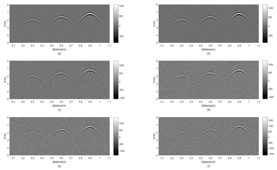
Figure 4.
Forward results with random noise: (a) add 5% random noise; (b) add 10% random noise; (c) add 15% random noise; (d) add 20% random noise; (e) add 25% random noise; (f) add 30% random noise.
2.3. Real Case Datasets
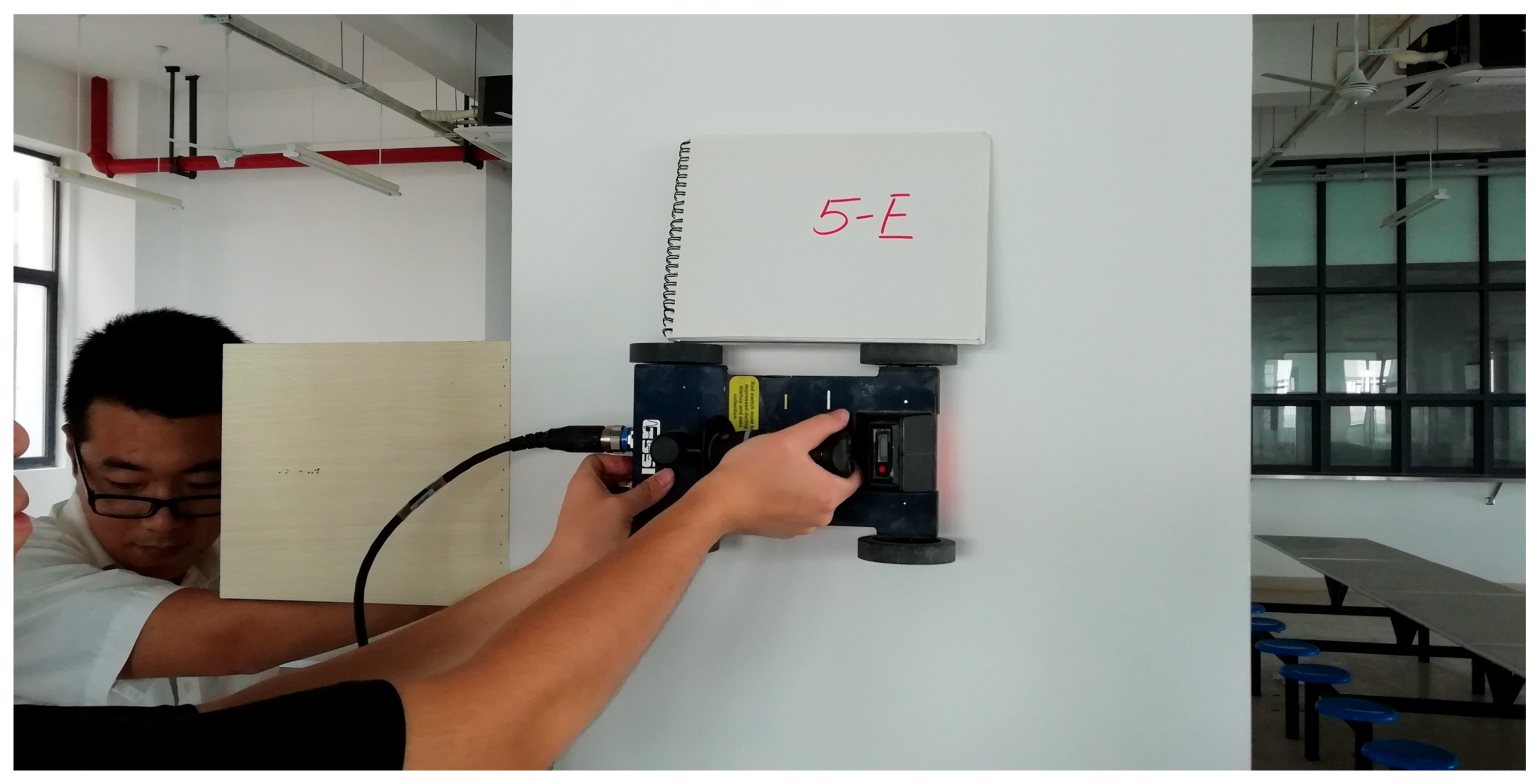
The site is located in a new camp on Changxing Island, Shanghai. To investigate the quality and scale of the reinforcement in the column or beam, GPR measurements were performed. The data was collected using GSSI sir-4000 GPR and an antenna with a center frequency of 2.6 GHZ. In particular, a small wooden bench was used to ensure that the measurements could be conducted from the column’s edge, as shown in Figure 5.

Figure 5.
Photo of the inspection using a wooden bench.
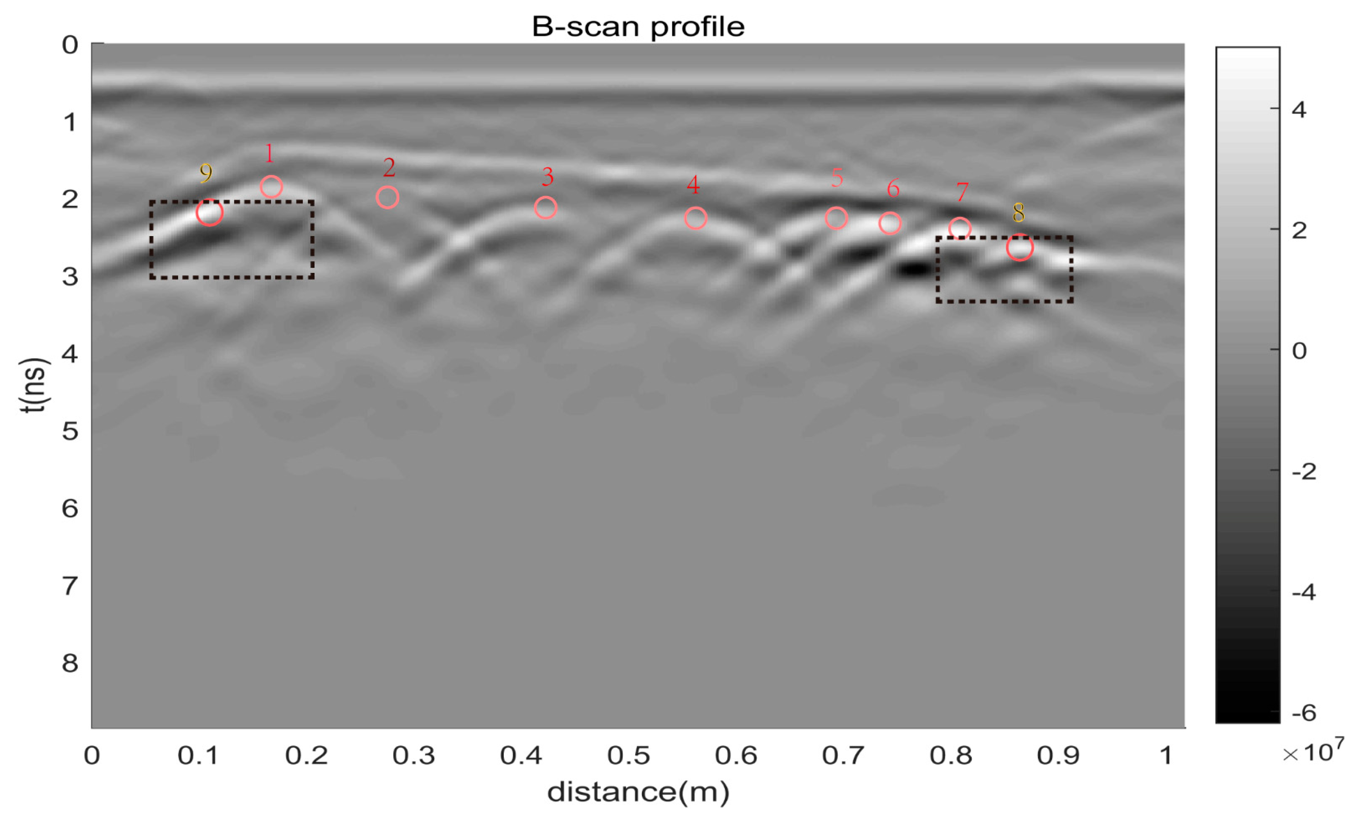
The specifications of all columns are the same, i.e., 0.8 m × 0.6 m. Column A was cut to verify the imaging result before testing. In data acquisition, the time window was set to 8.8541 ns; the samples per trace was 512; There were 408 traces in total, and the horizontal step was 2.5 mm. Figure 6 shows the B-scan profile of column A, in which the unit is V/m. The length of the survey line is 1.018 m. In this profile, nine hyperbolas (marked by red cycles and numbers) are identified, of which hyperbola 8 and hyperbola 9 are in doubt.
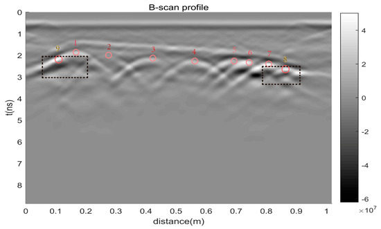
Figure 6.
The B-scan profile of the cut side.
At the same time, two black dotted boxes were utilized to identify hyperbola 8 and 9. Table 1 shows the locations and features of the identified hyperbolas. The four hyperbolas (number 1–4) are normal which denotes the typical hyperbola; the three hyperbolas (number 5–7) are almost overlapped; the hyperbola (number 8) is incomplete and smaller near to 0.9 m; the hyperbolas (number 1 and 9) are overlapped, moreover, the hyperbola (number 9) is hardly identifiable.

Table 1.
Hyperbolas of the B-scan profile of the cut side.
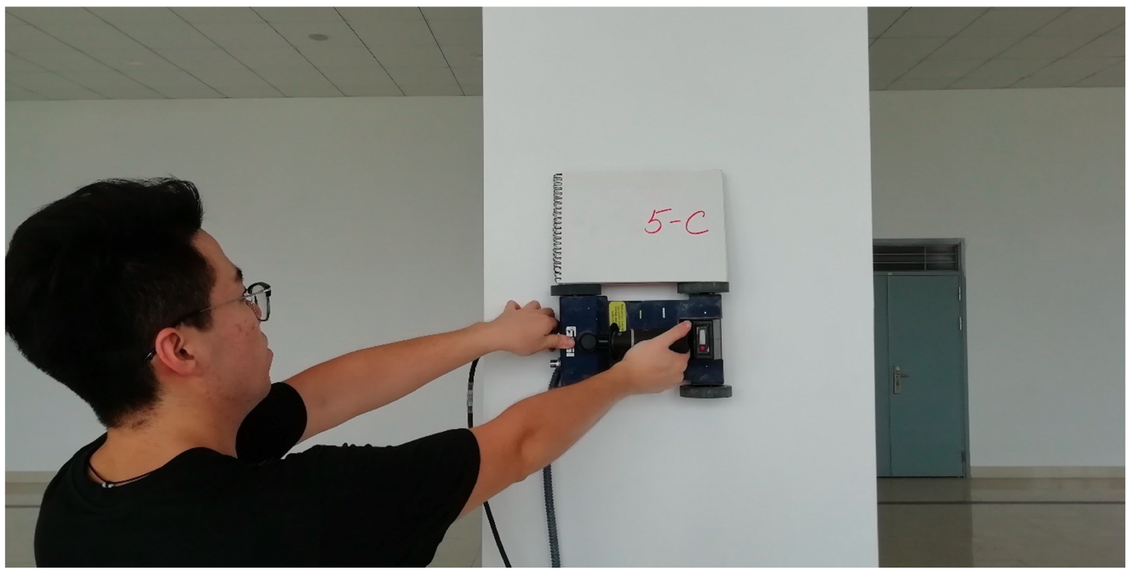
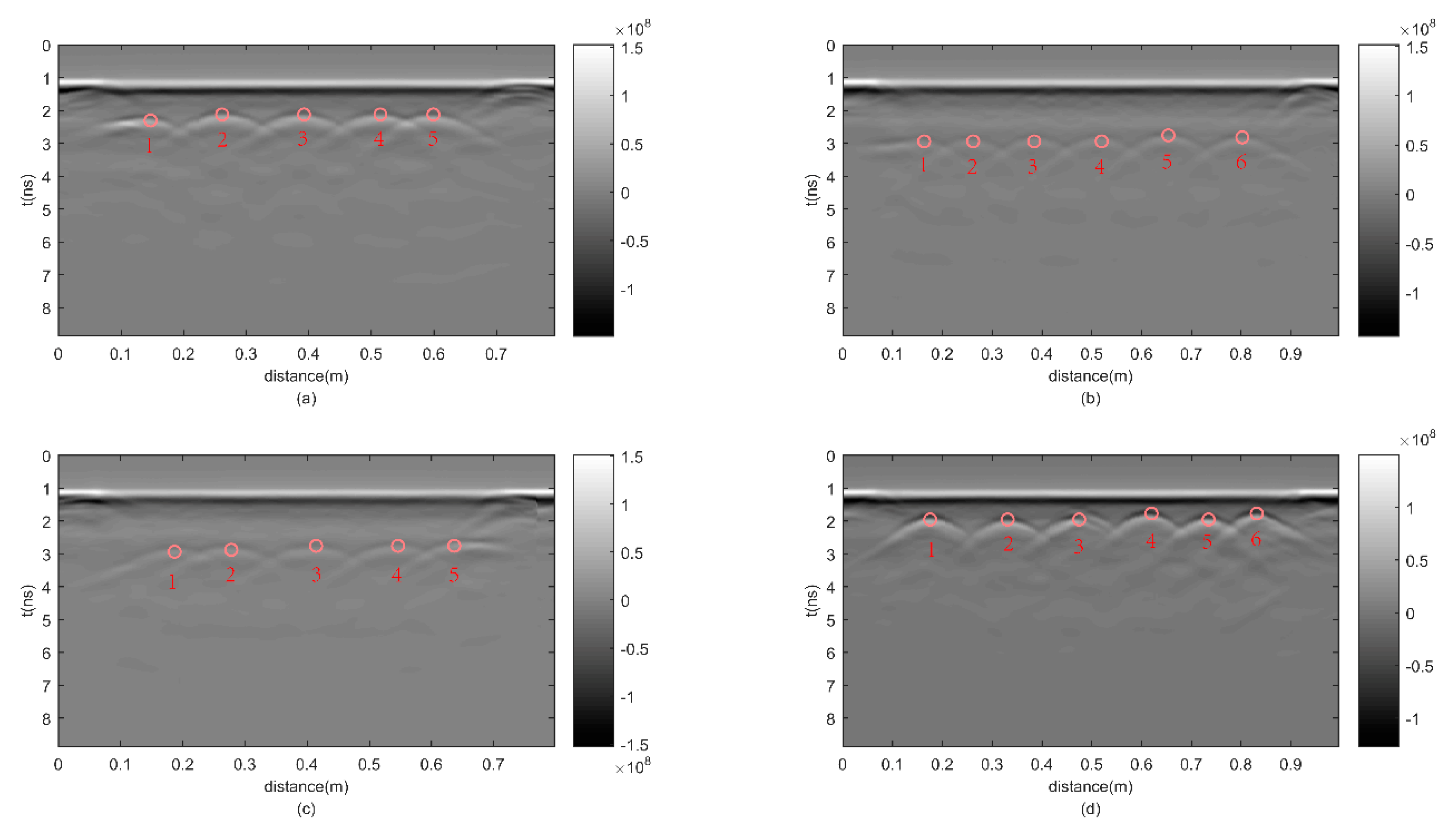
Figure 7 shows column B. The front side is 0.6 m as long as the backside. The left side, as well as the right side, is 0.8 m long. Figure 8 displays four clear B-scan profiles, of which the apexes of the hyperbolas have indications of red circles and numbers. The time window is 8.8541 ns, and the samples per trace are 512. Both the front and back profiles (Figure 8a,c) contain five hyperbolas, and both the left and right profiles (Figure 8b,d) include six hyperbolas. Table 2 shows the positions and features of the identified hyperbolas.

Figure 7.
Photo of column B.
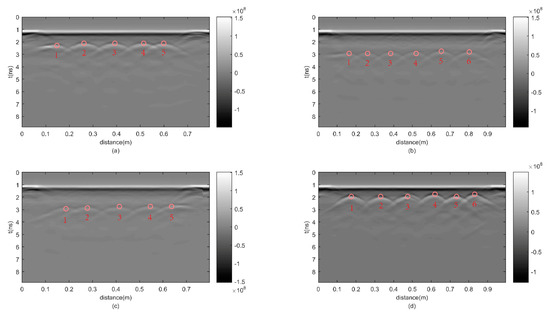
Figure 8.
Four B-scan profiles of column B: (a) the front side B-scan profile; (b) the right side B-scan profile; (c) the back side B-scan profile; (d) the left side B-scan profile.

Table 2.
Four B-scan profiles of column B.
In Figure 8a, the survey line is 0.7925 m long and consists of 318 traces. Note that the front side makes up the profile from 0.1 m to 0.7 m. The first hyperbola (number 1) is 0.1 m long horizontally from 0.1 m to 0.2 m. The second hyperbola (number 2) is 0.08 m longer, from 0.15 m to 0.33 m. Both hyperbolas (number 3 and 4) are as long as 0.15 m, ranging from 0.3 m to 0.45 m and from 0.4 m to 0.55 m, respectively. The fifth hyperbola (number 5) has a distance between 0.5 m and 0.7 m.
In Figure 8b, the survey line contains 399 traces, of which the length is 0.995 m. The right side is 0.8 m long from 0.1 m to 0.9 m. The first hyperbola (number 1) is 0.15 m long horizontally from 0.1 m to 0.25 m, which is straight from 0.1 m to 0.16 m. The second hyperbola (number 2) is almost as long as in Figure 8a and ranges from 0.16 m to 0.33 m. The third hyperbola (number 3) has a horizontal length of 0.15 m from 0.3 m to 0.45 m. The fourth hyperbola (number 4) and the fifth hyperbola (number 5) have a horizontal distribution from 0.4 m to 0.57 m and from 0.55 m to 0.72 m, respectively. The rightmost hyperbola (number 6) has the longest length ranging from 0.7 m to 0.9 m.
In Figure 8c, there are 320 traces in total, and the length of the survey line is 0.7975 m. The first hyperbola (number 1) is 0.15 m long from 0.08 m to 0.23 m. The second hyperbola (number 2), which is from 0.2 m to 0.35 m, has the same horizontal length as the previous one. The third hyperbola (number 3) is 0.17 m long horizontally from 0.3 m to 0.47 m. The fourth hyperbola (number 4) is 0.15 m long horizontally from 0.45 m to 0.6 m. The length of the fifth hyperbola (number 5) is equal to the last one from 0.55 m to 0.7 m, of which the hyperbola is straight between 0.65 m and the end.
In Figure 8d, there are 399 traces in total, and the survey line is 0.995 m as long as in Figure 8b. Six hyperbolas (number 1–6) have an identical horizontal length of 0.15 m, which range from 0.1 m to 0.25 m, 0.25 m to 0.4 m, 0.4 m to 0.55 m, 0.52 m to 0.67 m, 0.65 m to 0.8 m and 0.75 m to 0.9 m, respectively.
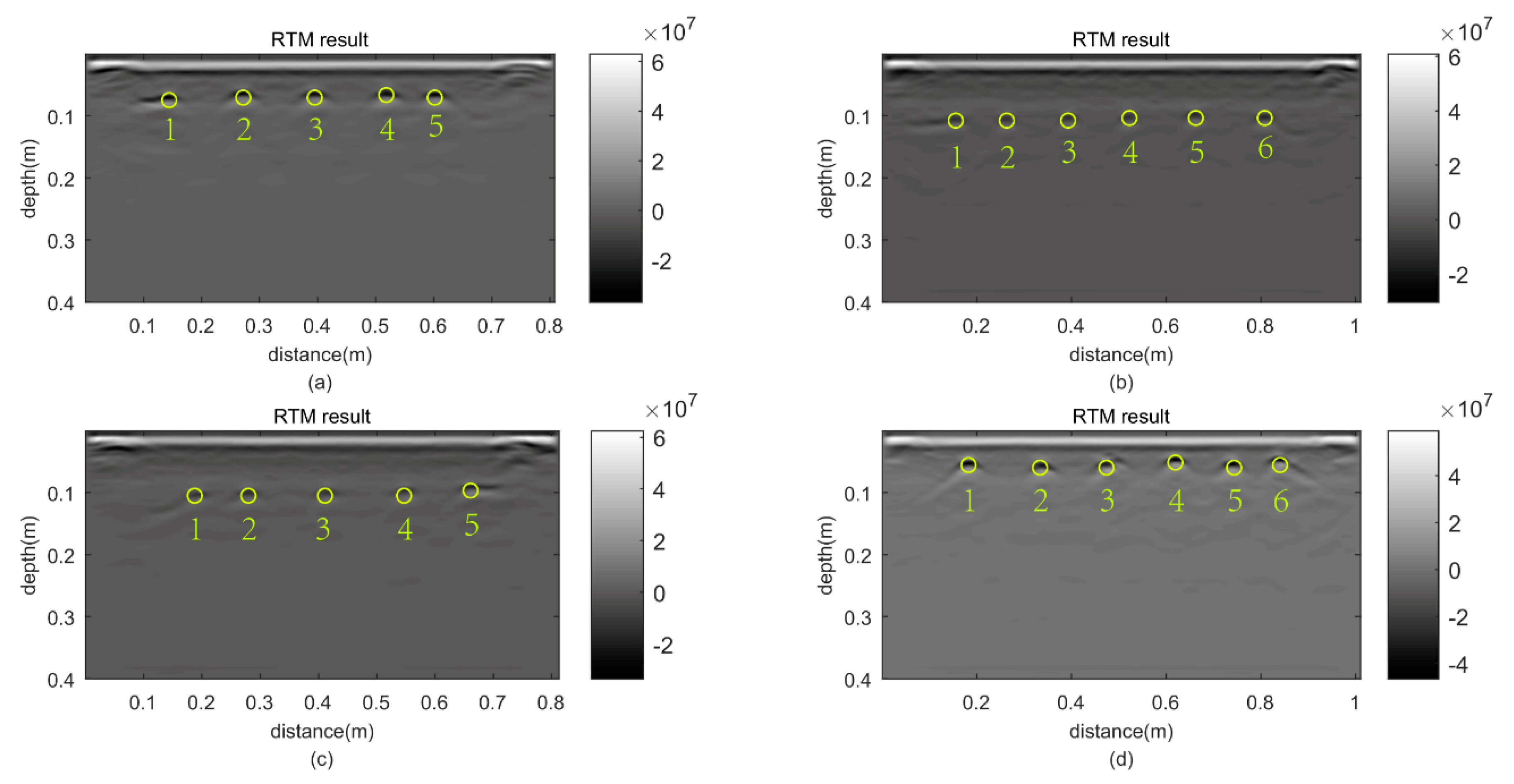
Figure 8 shows the accurate amount of the column and the approximate location of each steel bar. However, the precise depth of each reinforced bar is necessary for the determination of the reinforced structure. For the determination and localization of the reinforced bars, we adopted the RTM algorithm to process the data of the four B-scan profiles.
3. Results
3.1. Synthetic Data Test
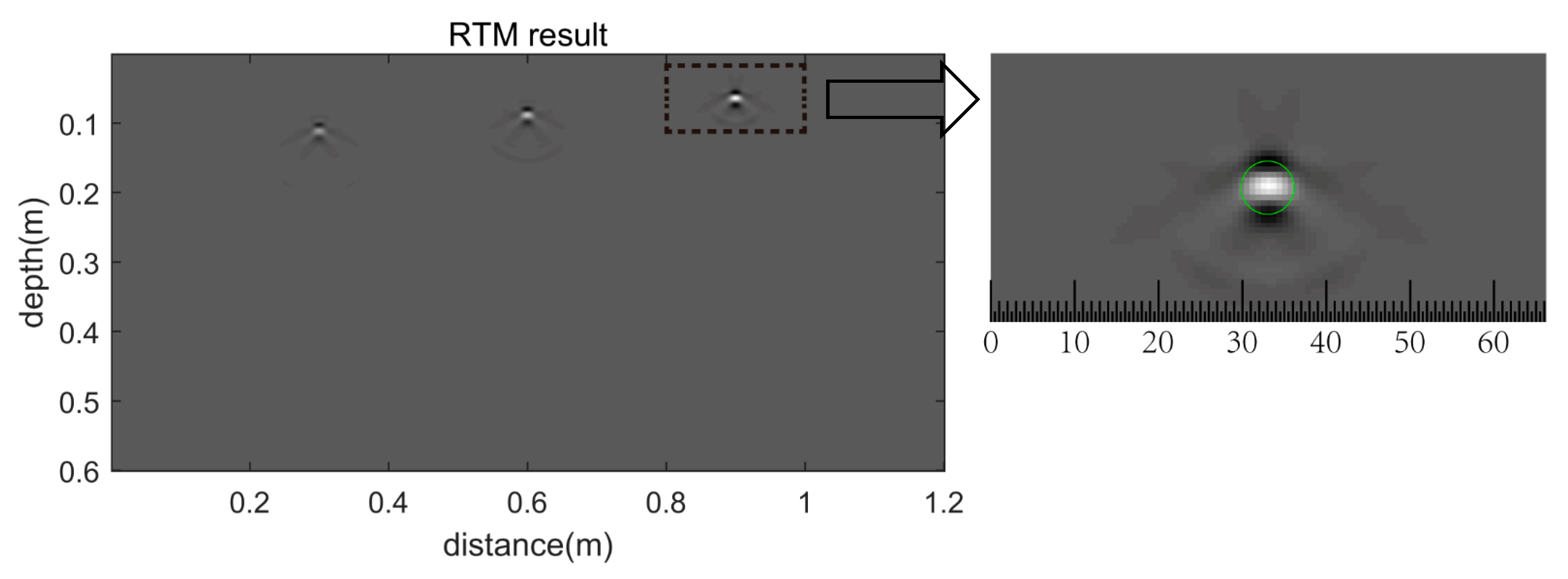
Figure 9 shows the imaging results of the synthetic GPR profile presented in Figure 3. We can see that the energy of the hyperbola converges precisely to a region consistent with the scale of the reinforced steel bars. The depth and horizontal position of the left point are 0.1 m and 0.3 m, respectively; the depth and horizontal position of the middle one are 0.075 m and 0.6 m, respectively; the depth and horizontal position of the right one are 0.5 m and 0.9 m. For quantifying the diameters of rebars, an area inside the black-dotted box was enlarged. As the arrow points out, the image inside the box was enlarged into the detail window. We used a circle to mark the identified rebar. Moreover, we scaled the length of the detail window to estimate the diameter.
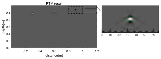
Figure 9.
The imaging result of the synthetic data.
The corresponding imaging results of Figure 4a,f are shown in Figure 10a–f, respectively. The unit in all results is V/m. The depths and horizontal positions of the identified points are (0.1 m, 0.3 m), (0.075 m, 0.6 m), and (0.05 m, 0.9 m) from left to right, respectively, which are identical to those in the real model.
3.2. Real Field Data Test
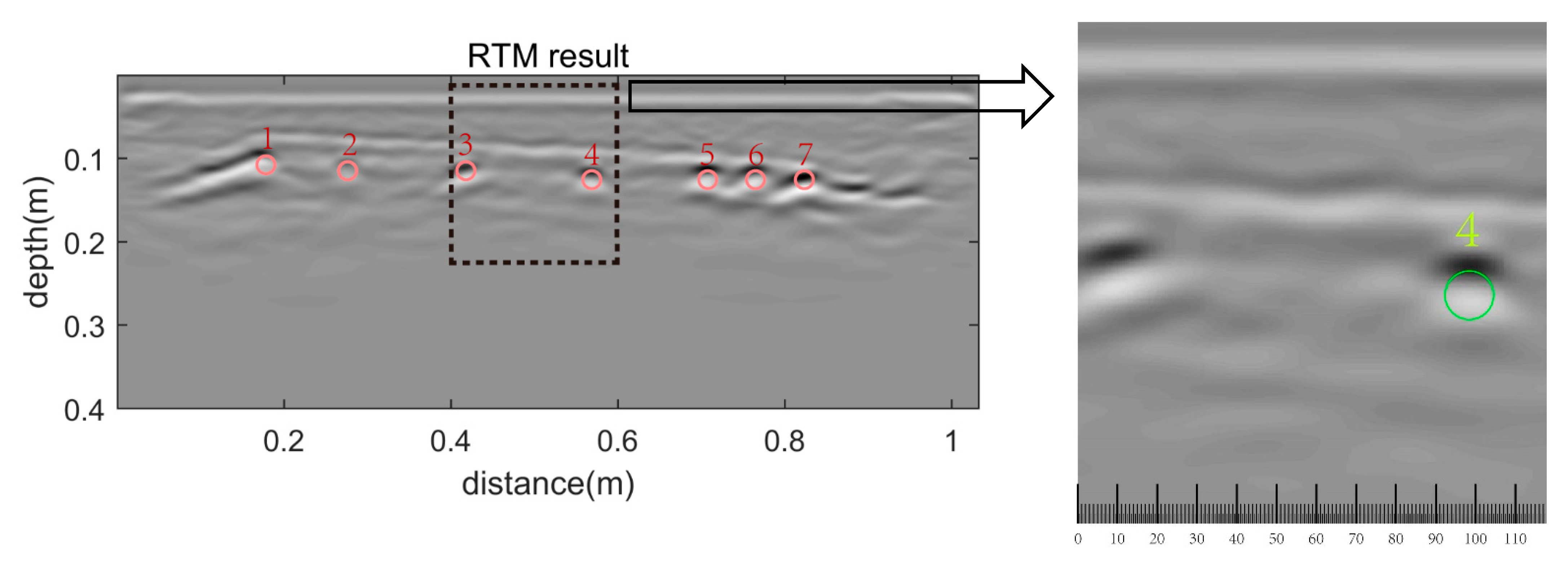
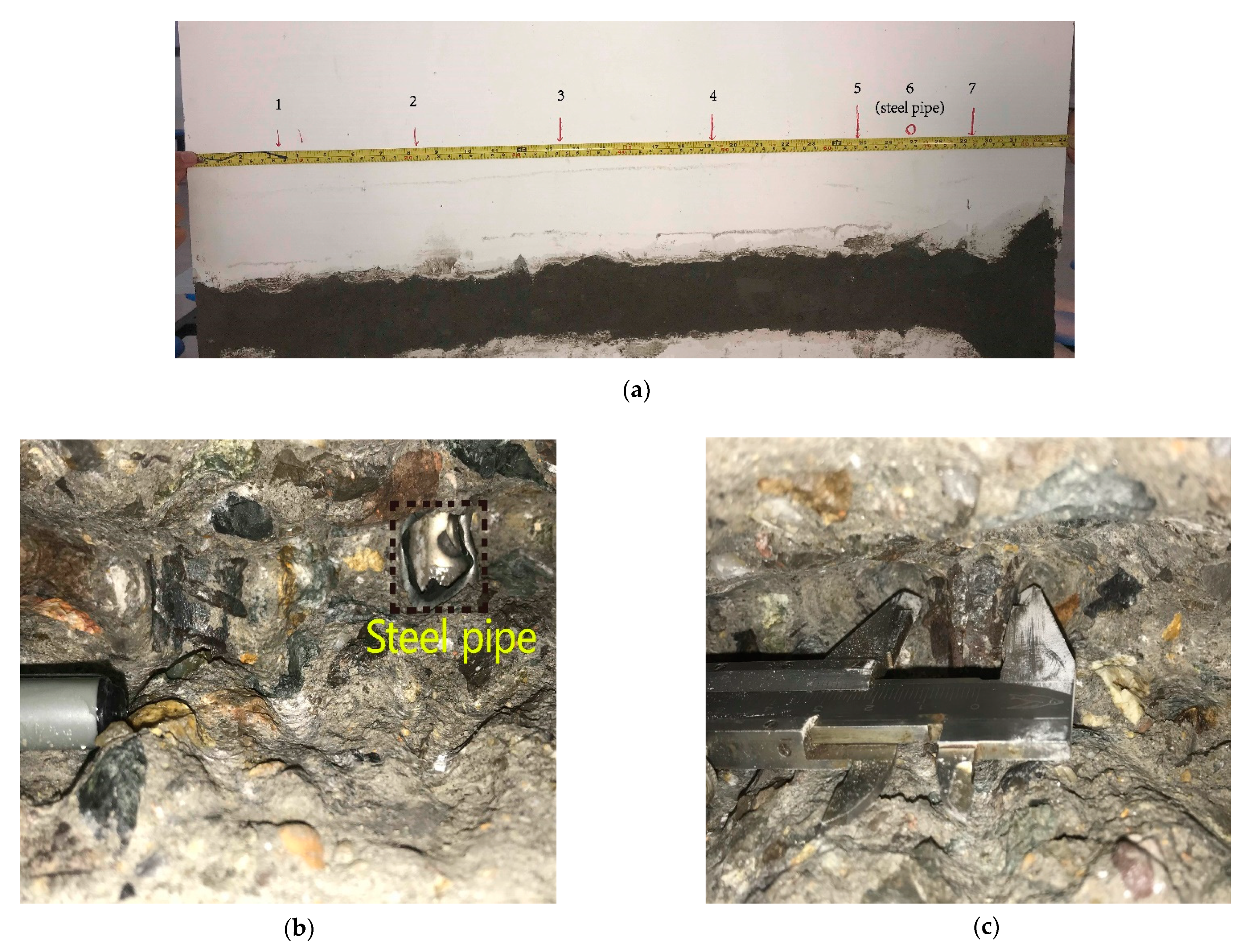
In this paper, the horizontal axes of all imaging results are 0.01 m longer, and the maximum depth is 0.4 m. The size of the grid is 0.5 mm x 0.5 mm, and the sampling interval is reduced to one-hundredth of the original to satisfy the time stability condition. Figure 11 shows the imaging result of the cut column. We identified and marked seven reinforcements (number 1–7) by red circles, of which the positions are (0.16 m, 0.11 m), (0.28 m, 0.12 m), (0.42 m, 0.12 m), (0.56 m, 0.13 m), (0.7 m, 0.13 m), (0.75 m, 0.13 m) and (0.81 m, 0.13 m), respectively. Middle hyperbolas (number 2–6 in Figure 6) collapsed into clouds (number 2–6 in Figure 11) except that the leftmost one, as well as the rightmost one, converged to a striped shape. For quantifying the diameter, we selected an area, i.e., the area inside a black-dotted box. Rebar 4 is marked by a green circle. Table 3 shows the positions and features of the identified rebars. As shown in Figure 12a, the cut side is 0.8 m long. The cut column in Figure 12a demonstrates that the positions of rebars in the imaging result are well retrieved. Notably, as shown in Figure 12b, the black-dotted box surrounds the steel pipe, and the right hyperbola (number 6) is generated by a steel pipe. Figure 12c shows that the real diameter of the rebar is approximately 22 mm.

Figure 11.
The imaging result of the cut side.

Table 3.
Identified reinforcements of the imaging result of the cut side.
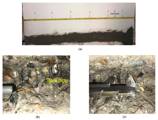
Figure 12.
Photo of column A: (a) The appearance of the cut side; (b) the steel pipe; (c) the diameter of one reinforcement.
Figure 13a–d show the imaging results of the profiles in Figure 8a–d, respectively. Similarly, the unit is V/m. We marked all identified rebars by circles and numbers. Table 4 shows the quantity, positions, and features of the identified rebars. Figure 13a,c contain one less reinforcement than that in Figure 13b,d. The depths of the identified reinforced bars in Figure 13a,d are less than 10 cm, which are mainly 0.6 m and 0.5 m, respectively. Conversely, the depths of rebars in Figure 13b,c are more than 10 cm, which are mainly 0.11 m. In Figure 13 b,c, the collapsed energy is mainly dotted except that the first one in Figure 13b and the fifth one in Figure 13c are striped. The focused hyperbolas are mainly curved in Figure 13a,d except for the first one in Figure 13a which is striped.
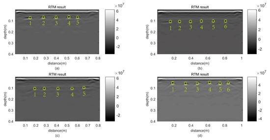
Figure 13.
The four imaging results of column B: (a) the front side; (b) the right side; (c) the back side; (d) the left side.

Table 4.
Identified reinforcements of the imaging result of column B.
4. Discussion
In the synthetic data test, the locations of identified rebars are (0.3 m, 0.1 m), (0.6 m, 0.75 m), and (0.9 m, 0.5 m), respectively, which are consistent with the real ones. For quantifying the diameter, we enlarged an area inside a black-dotted box. As shown in Figure 9, the rebar is marked. Notably, the box is 0.2 m wide, i.e., the real diameter must be from conversion. By conversion, the diameter of the identified rebar is approximately 24.2 mm and the error is 0.2 mm. This result validates the ability of the RTM algorithm. By noisy experiment, we find that the positions of identified rebars are equal to the previous ones. This result proves the stability of the RTM algorithm.
In the paper, the dataset of the cut column A is provided first. We identified nine hyperbolas of which hyperbola 1–7 are clear. Hyperbola 8 is small but curved so that it, as well as hyperbola 9, is in doubt. The hyperbolic energy (number 9) is very weak and overlapped with hyperbola 1. Specially, we made use of black-dotted boxes to identify hyperbola 8 and 9. However, the migration image shows seven identified rebars that correspond to hyperbola 1–7, i.e., we identified disturbing energy in mistake for hyperbolas. To verify the capability of the RTM algorithm on the real case dataset, we cut the column. As shown in Figure 12, the horizontal distance of the seven bars are 8.3 cm, 21 cm, 34 cm, 48.8 cm, 63 cm, 68.5 cm, and 74.5 cm, respectively. Table 3 shows that the relative locations of the identified rebars are consistent with those of the real ones. Moreover, the identified rebar (number 6) is a steel pipe. To quantify the diameter, we selected one black-dotted box that surrounded the identified rebar 3 and 4. Obviously, rebar 4 has been retrieved better. By conversion, the interpreted diameter is about 20.4 mm. The error is 1.6 mm. Nevertheless, the other rebars are retrieved worse, i.e., there exists some degree of error that has an influence on the interpretation. On the other hand, the diffraction wave is suppressed well.
Based on the imaging result of column A, we utilized the RTM algorithm to process the real case datasets of column B which included four sides. From the B-scan profiles, the hyperbolic energy in Figure 8a,d are stronger. Clearly, the energy of the diffraction wave is more powerful with less depth of the rebar. In Figure 13b,c, the hyperbolas collapse better. The results prove the ability of suppressing the diffraction wave of the RTM algorithm.
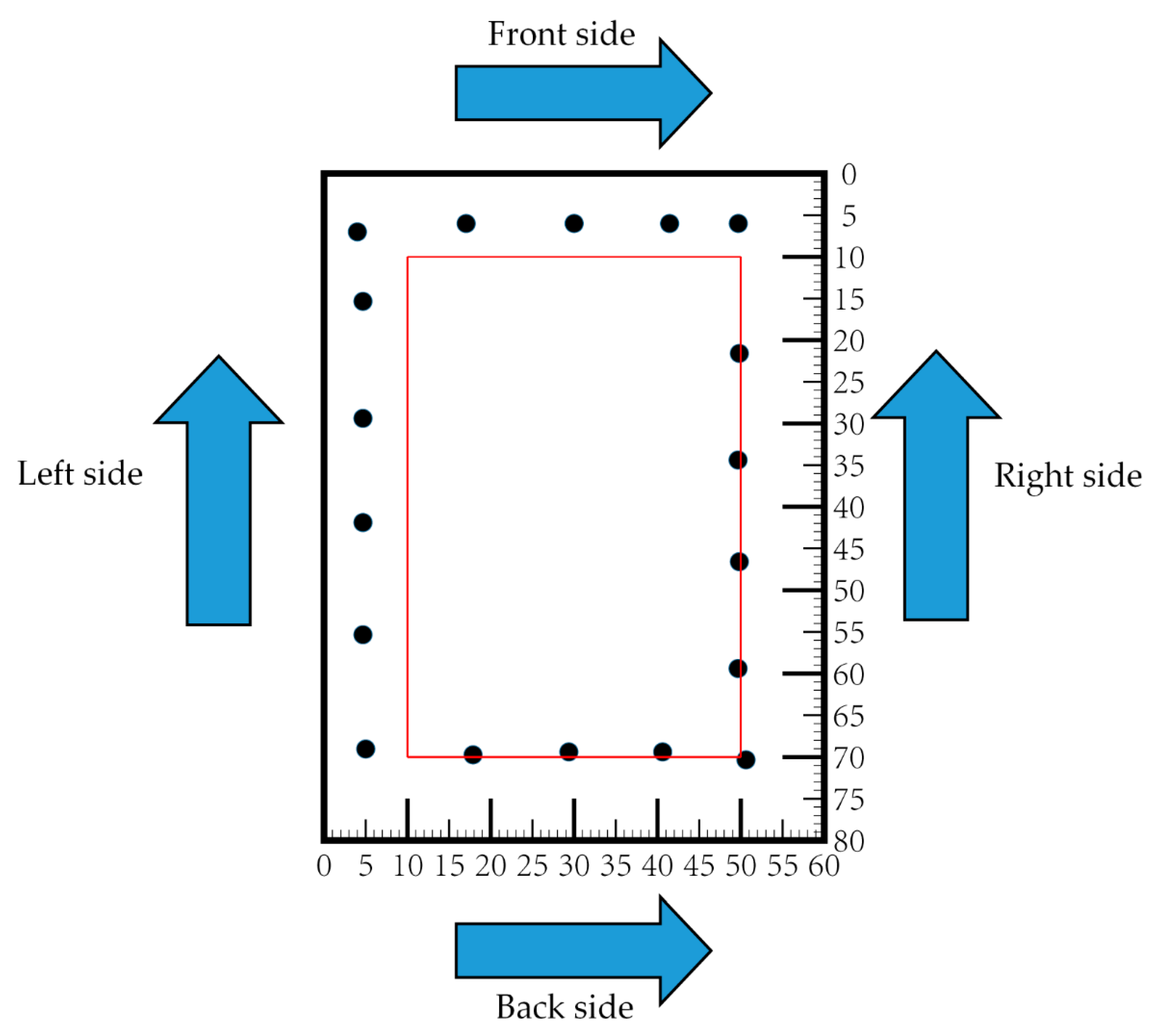
Figure 14 shows the reinforced concrete structure inferred from the imaging results shown in Figure 13. The arrow denotes the direction of the survey line and the red rectangle represents the position of 10 cm below the column surface; the black circles represent the steel bar. As shown in Figure 14, the left and front thicknesses of the protective layer are less than 10 cm; the right and back thicknesses are more than 10 cm. However, the cover thickness of reinforcements in a concrete structure is required to be less than 10 cm.
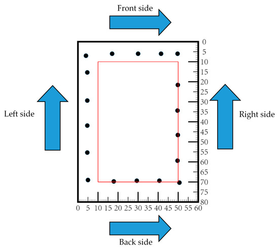
Figure 14.
The interpreted reinforced concrete structure.
5. Conclusions
Here, we carried out GPR measurements combined with the RTM algorithm in the localization of reinforcements. We first used a synthetic example to test the ability of the proposed strategy. After the RTM processing, the hyperbolas converged to the region consistent with the real model. Even for noisy data, whose signal-to-noise ratio is too low to identify the response of the hyperbolas, the diffraction energy was collapsed correctly to the positions of the rebars. In addition, the error between the estimated diameter and the real diameter was less than 1 mm. These results demonstrate the capability of the RTM algorithm in reinforcement detection.
Following this, we performed an on-site test to determine the quantity and locations of reinforced steel bars of buildings. Before measurements, we tested the proposed strategy again on a cut column. The migration image shows that the hyperbolic reflections are well focused. The interpreted quantity and positions of the rebars were verified by the real result on column A. The consistency between the migrated result and the fundamental structure of the column further shows the effectiveness of the strategy. However, the error of diameters reaches 1.6 mm, i.e., 7.2%. Finally, we used the RTM algorithm to process the GPR data measured from column B. The results show that the diffraction wave is well suppressed. According to the imaging result of the four sides, we retrieved a reinforced concrete structure, which illustrates that the protective layer thickness of the column is partly qualified.
In summary, the proposed RTM algorithm can help with suppressing the hyperbolic reflections to localize and detect concrete reinforced bars. However, the accuracy of estimation of diameters on real case datasets is a problem. We will investigate other methods to improve the accuracy.
On the other hand, the reinforced concrete structural problem is related to the prevention and the solution of construction safety hazards. When the signal attenuation is significant, energy compensation should be incorporated with the RTM to better resolve the concrete structure.
Author Contributions
Conceptualization, R.S. and Y.Z.; methodology, R.S.; software, R.S.; validation, R.S., S.H., and W.B.; formal analysis, R.S. and B.L.; investigation, R.S., W.B., and B.L.; resources, R.S.; data curation, R.S.; writing—original draft preparation, R.S.; writing—review and editing, S.H. and Y.Z.; visualization, R.S.; supervision, Y.Z.; project administration, Y.Z.; funding acquisition, Y.Z. All authors have read and agreed to the published version of the manuscript.
Funding
This research was sponsored by the Natural Science Foundation of China (No. 41774124).
Institutional Review Board Statement
Not applicable.
Informed Consent Statement
Not applicable.
Data Availability Statement
The data presented in this study are available on request from the corresponding author. The data are not publicly available due to some special reasons.
Conflicts of Interest
The authors declare no conflict of interest.
References
- Lambot, S.; Slob, E.C.; Van den Bosch, I.; Stockbroeckx, B.; Vanclooster, M. Modeling of ground-penetrating Radar for accurate characterization of subsurface electric properties. IEEE Trans. Geosci. Remote Sens. 2004, 42, 2555–2568. [Google Scholar] [CrossRef]
- Lunt, I.A.; Hubbard, S.S.; Rubin, Y. Soil moisture content estimation using ground-penetrating radar reflection data. J. Hydrol. 2005, 307, 254–269. [Google Scholar] [CrossRef]
- Loke, M.H.; Chambers, J.E.; Rucker, D.F.; Kuras, O.; Wilkinson, P.B. Recent developments in the direct-current geoelectrical imaging method. J. Appl. Geophys. 2013, 95, 135–156. [Google Scholar] [CrossRef]
- Gader, P.D.; Mystkowski, M.; Zhao, Y.X. Landmine detection with ground penetrating radar using hidden Markov models. IEEE Trans. Geosci. Remote Sens. 2001, 39, 1231–1244. [Google Scholar] [CrossRef]
- Torrione, P.A.; Morton, K.D.; Sakaguchi, R.; Collins, L.M. Histograms of Oriented Gradients for Landmine Detection in Ground-Penetrating Radar Data. IEEE Trans. Geosci. Remote Sens. 2014, 52, 1539–1550. [Google Scholar] [CrossRef]
- Wilson, J.N.; Gader, P.; Lee, W.; Frigui, H.; Ho, K.C. A Large-Scale Systematic Evaluation of Algorithms Using Ground-Penetrating Radar for Landmine Detection and Discrimination. IEEE Trans. Geosci. Remote Sens. 2007, 45, 2560–2572. [Google Scholar] [CrossRef]
- Demanet, D.; Renardy, F.; Vanneste, K.; Jongmans, D.; Camelbeeck, T.; Meghraoui, M. The use of geophysical prospecting for imaging active faults in the Roer Graben, Belgium. Geophysics 2001, 66, 78–89. [Google Scholar] [CrossRef]
- Vasco, D.W.; Peterson, J.E.; Lee, K.H. Ground-penetrating radar velocity tomography in heterogeneous and anisotropic media. Geophysics 1997, 62, 1758–1773. [Google Scholar] [CrossRef]
- Lai, J.L.; Xu, Y.; Zhang, X.P.; Xiao, L.; Yan, Q.; Meng, X.; Zhou, B.; Dong, Z.H.; Zhao, D. Comparison of dielectric properties and structure of lunar regolith at Chang’e-3 and Chang’e-4 landing sites revealed by ground-penetrating radar. Geophys. Res. Lett. 2019, 46, 12783–12793. [Google Scholar] [CrossRef]
- Zhang, L.; Zeng, Z.F.; Li, J.; Lin, J.Y.; Hu, Y.S.; Wang, X.G.; Sun, X.D. Simulation of the Lunar Regolith and Lunar-Penetrating Radar Data Processing. IEEE J. Sel. Top. Appl. Earth Obs. Remote Sens. 2018, 11, 655–663. [Google Scholar] [CrossRef]
- Grandjean, G.; Gourry, J.C.; Bitri, A. Evaluation of GPR techniques for civil-engineering applications: Study on a test site. J. Appl. Geophys. 2000, 45, 141–156. [Google Scholar] [CrossRef]
- Lai, W.W.L.; Derobert, X.; Annan, P. A review of Ground Penetrating Radar application in civil engineering: A 30-year journey from Locating and Testing to Imaging and Diagnosis. NDT E Int. 2018, 96, 58–78. [Google Scholar] [CrossRef]
- Hugenschmidt, J. Concrete bridge inspection with a mobile GPR system. Constr. Build. Mater. 2002, 16, 147–154. [Google Scholar] [CrossRef]
- Leucci, G. Ground Penetrating Radar: An Application to Estimate Volumetric Water Content and Reinforced Bar Diameter in Concrete Structures. J. Adv. Concr. Technol. 2012, 10, 411–422. [Google Scholar] [CrossRef]
- Tosti, F.; Ferrante, C. Using Ground Penetrating Radar Methods to Investigate Reinforced Concrete Structures. Surv. Geophys. 2020, 41, 485–530. [Google Scholar] [CrossRef]
- Zhou, F.; Chen, Z.C.; Liu, H.; Cui, J.; Spencer, B.E.; Fang, G.Y. Simultaneous Estimation of Rebar Diameter and Cover Thickness by a GPR-EMI Dual Sensor. Sensors 2018, 18, 2969. [Google Scholar] [CrossRef] [PubMed]
- Chang, C.W.; Lin, C.H.; Lien, H.S. Measurement radius of reinforcing steel bar in concrete using digital image GPR. Constr. Build. Mater. 2009, 23, 1057–1063. [Google Scholar] [CrossRef]
- Shaw, M.R.; Molyneaux, T.C.K.; Millard, S.G.; Taylor, M.J.; Bungey, J.H. Assessing bar size of steel reinforcement in concrete using ground penetrating radar and neural networks. Insight Non Destruct. Test. Cond. Monit. 2003, 45, 813–816. [Google Scholar] [CrossRef]
- Tesic, K.; Baricevic, A.; Serdar, M. Non-Destructive Corrosion Inspection of Reinforced Concrete Using Ground-Penetrating Radar: A Review. Materials 2021, 14, 975. [Google Scholar] [CrossRef] [PubMed]
- Tarussov, A.; Vandry, M.; De La Haza, A. Condition assessment of concrete structures using a new analysis method: Ground-penetrating radar computer-assisted visual interpretation. Constr. Build. Mater. 2013, 38, 1246–1254. [Google Scholar] [CrossRef]
- Liu, H.; Lin, C.X.; Cui, J.; Fan, L.S.; Xie, X.Y.; Spencer, B.F. Detection and localization of rebar in concrete by deep learning using ground penetrating radar. Autom. Constr. 2020, 118, 103279. [Google Scholar] [CrossRef]
- Giannakis, I.; Giannopoulos, A.; Warren, C. A Machine Learning Scheme for Estimating the Diameter of Reinforcing Bars Using Ground Penetrating Radar. IEEE Geosci. Remote Sens. Lett. 2021, 18, 461–465. [Google Scholar] [CrossRef]
- Zadhouse, H.; Giannopoulos, A.; Giannakis, I. Optimising the Complex Refractive Index Model for Estimating the Permittivity of Heterogeneous Concrete Models. Remote Sens. 2021, 13, 723. [Google Scholar] [CrossRef]
- Kalogeropoulos, A.; Van der Kruk, J.; Hugenschmidt, J.; Bikowski, J.; Bruhwiler, E. Full-waveform GPR inversion to assess chloride gradients in concrete. NDT E Int. 2013, 57, 74–84. [Google Scholar] [CrossRef]
- Alani, A.M.; Giannakis, I.; Zou, L.L.; Lantini, L.; Tosti, F. Reverse-time migration for evaluating the internal structure of tree-trunks using ground-penetrating radar. NDT E Int. 2020, 115, 102294. [Google Scholar] [CrossRef]
- Ozdemir, C.; Demirci, S.; Yigit, E.; Yilmaz, B. A Review on Migration Methods in B-Scan Ground Penetrating Radar Imaging. Math. Probl. Eng. 2014, 2014, 280738. [Google Scholar] [CrossRef]
- Bitri, A.; Grandjean, G. Frequency–wavenumber modelling and migration of 2D GPR data in moderately heterogeneous dispersive Media. Geophys. Prospect. 1998, 46, 287–301. [Google Scholar] [CrossRef]
- Moran, M.L.; Greenfield, R.J.; Arcone, S.A.; Delaney, A.J. Multidimensional GPR array processing using Kirchhoff migration. J. Appl. Geophys. 2000, 43, 281–295. [Google Scholar] [CrossRef]
- Bradford, J.H. Reverse-time prestack depth migration of GPR data from topography for amplitude reconstruction in complex environments. J. Earth Sci. 2015, 26, 791–798. [Google Scholar] [CrossRef]
- Fisher, E.; Mcmechan, G.A.; Annan, A.P.; Cosway, S.W. Examples of reverse-time migration of single-channel, ground-penetrating radar profiles. Geophysics 1992, 57, 577–586. [Google Scholar] [CrossRef]
- Zhou, H.; Sato, M.; Liu, H.J. Migration velocity analysis and prestack migration of common-transmitter GPR data. IEEE Trans. Geosci. Remote Sens. 2005, 43, 86–91. [Google Scholar] [CrossRef]
- Liu, S.X.; Lei, L.L.; Fu, L.; Wu, J.J. Application of pre-stack reverse time migration based on FWI velocity estimation to ground penetrating radar data. J. Appl. Geophys. 2014, 107, 1–7. [Google Scholar] [CrossRef]
- Liu, H.; Long, Z.J.; Han, F.; Fang, G.Y.; Liu, Q.H. Frequency-Domain Reverse-Time Migration of Ground Penetrating Radar Based on Layered Medium Green’s Functions. IEEE J. Sel. Top. Appl. Earth Obs. Remote Sens. 2018, 11, 2957–2965. [Google Scholar] [CrossRef]
- Huo, J.J.; Zhao, Q.; Zhao, B.Z.; Liu, L.B.; Ma, C.G.; Guo, J.Y.; Xie, L.H. Energy Flow Domain Reverse-Time Migration for Borehole Radar. IEEE Trans. Geosci. Remote Sens. 2019, 57, 7221–7231. [Google Scholar] [CrossRef]
- Irving, J.; Knight, R. Numerical modeling of ground-penetrating radar in 2-D using MATLAB. Comput. Geosci. 2006, 32, 1247–1258. [Google Scholar] [CrossRef]
Publisher’s Note: MDPI stays neutral with regard to jurisdictional claims in published maps and institutional affiliations. |
© 2021 by the authors. Licensee MDPI, Basel, Switzerland. This article is an open access article distributed under the terms and conditions of the Creative Commons Attribution (CC BY) license (https://creativecommons.org/licenses/by/4.0/).

