Abstract
High-precision 3D maps play an important role in autonomous driving. The current mapping system performs well in most circumstances. However, it still encounters difficulties in the case of the Global Navigation Satellite System (GNSS) signal blockage, when surrounded by too many moving objects, or when mapping a featureless environment. In these challenging scenarios, either the global navigation approach or the local navigation approach will degenerate. With the aim of developing a degeneracy-aware robust mapping system, this paper analyzes the possible degeneration states for different navigation sources and proposes a new degeneration indicator for the point cloud registration algorithm. The proposed degeneracy indicator could then be seamlessly integrated into the factor graph-based mapping framework. Extensive experiments on real-world datasets demonstrate that the proposed 3D reconstruction system based on GNSS and Light Detection and Ranging (LiDAR) sensors can map challenging scenarios with high precision.
Keywords:
3D reconstruction; LiDAR; GNSS; scan matching; factor graph; degeneracy-aware factors; loop closure 1. Introduction
Rapid progress has been witnessed in the field of unmanned ground vehicles (UGVs) [1,2]. Autonomous driving is expected to address transportation problems such as road accidents and traffic congestion [3,4]. Among those enabling technologies, the creation and utilization of a high-precision map play an important role [5]. The high-precision map differs from the traditional map not only in its higher accuracy but also in that it contains much more environmental information, which will benefit other modules [6].
The high-precision map should be accurate both globally and locally. At the global scale, the map should be well aligned with the Global Navigation Satellite System (GNSS) trajectory [7]. Locally, the map should fully capture the local details of the surroundings, and the map’s accuracy should be at the centimeter level [8]. To meet these requirements, the mapping system should combine the global navigation approaches with local navigation approaches. Whilst the global navigation information could come from the GNSS system, the local navigation information could be obtained from the Inertial Measurement Unit (IMU), wheel odometer, or Light Detection and Ranging (LiDAR) odometry. However, both types of navigation information may become inaccurate in some circumstances [1,9].
For the global navigation information, the GNSS signal might become inaccurate due to the blockage of tall buildings or the well-known multi-path effect [10]. It may even become unavailable in certain scenarios, such as under bridges, in tunnels, in underground parking lots, etc. For the local navigation approaches, the wheel odometer may become inaccurate in the case of slippage [11]. The LiDAR odometry may also become inaccurate in a featureless environment or when surrounded by too many moving objects [9,12]. Therefore, an ideal mapping system should be capable of detecting the degeneracy state for both navigation approaches, and a robust fusion approach should be designed.
In this paper, we propose to use the factor graph as the fusion framework. The factor graph is a probabilistic framework that could capably handle the uncertainties of different navigation approaches and integrate the different sources of navigation information in a principled way [13].
We thoroughly analyze the different factors contained in the proposed factor graph and design approaches that could estimate the degeneracy state for each factor. The degeneracy state is then transformed to adjust the information matrix for each factor. Therefore, the proposed fusion framework automatically assigns high confidence to those highly confident factors and weakens the influence of those degenerate factors.
We test the proposed mapping system in several challenging scenarios with two types of vehicles equipped with two different kinds of LiDAR, as shown in Figure 1. The testing scenarios include over a high bridge with busy traffic, in an underground parking lot, and a featureless off-road environment. Experimental results show that the proposed mapping framework could overcome the influence of dynamic objects, the GNSS signal outage, and the scan matching degradation. All the testing scenarios are mapped with high precision. The maps built are also shown in Figure 1. To make the mapping system more complete, we also discuss problems regarding loop closure detection and automatic map update and extension.

Figure 1.
The fully automated 3D mapping system for self-driving vehicles in challenging scenarios. Two platforms equipped with two types of multi-channel LiDARs are shown on the left. The testing scenarios include busy urban environments with high bridges (a–c), underground parking lots (d), open scenarios (e), and featureless off-road scenarios (f). Maps are colored by altitude.
In summary, we have made the following contributions in this paper:
- A factor graph-based fusion framework is proposed which could suitably integrate the global navigation information with local navigation information in a probabilistic way.
- A comprehensive degeneration analysis is performed for both the global and the local navigation approach. A new robust degeneration indicator is proposed for the local navigation approach which could reliably estimate the degeneration state of the scan matching algorithm. The degeneration state is then incorporated into the factor graph, thus enabling a more robust, degeneration-aware fusion approach.
- An improved submap-to-submap matching method is used to estimate loop closure constraints. The loop closure constraint can be reliably estimated even with a large initial position offset or a limited overlap field of view.
- The proposed mapping system has been extensively tested on real-world datasets in several challenging scenarios, including busy urban scenarios, featureless off-road scenarios, high bridges, highways, and large-scale settings. Experimental results confirmed the effectiveness of the mapping system.
2. Related Work
LiDAR-based mapping has been extensively studied [1,14]. A complete mapping system includes at least the following modules: the front-end scan matching, the loop closure detection, and the back-end optimization. This paper reviews related works from the following aspects.
2.1. Scan Matching
As the basis of the LiDAR-based mapping system, scan matching methods can be generally divided into two categories: local approaches and global approaches [12]. Iterative Closest Point (ICP) and its variants [15,16] are widely used local scan matching approaches. Point-to-point, point-to-plane, or plane-to-plane distances are usually applied to measure spatial distances of local structures extracted from two scans. The local structure could also be approximated using the Gaussian model [17]. The transformation is then estimated by minimizing the distances of corresponding local structures. As a widely used approach in recent years, Lidar Odometry and Mapping (LOAM) [18] firstly extracts corner points and surface points based on the local geometric structures. The point-to-line distance and the point-to-plane distance are then separately applied to these corner points and surface points. Compared with these local approaches, the Correlative Scan Matching (CSM) [19] is a popular global scan matching approach that treats the scan as a whole. It enumerates all the possible transformations and selects the best one based on the global distance measure. Due to its heavy computational load, CSM is not suitable for 3D matching. Fu et al. [12] proposed to combine the global scan matching approaches with local scan matching approaches and obtained competitive results in off-road environments.
2.2. Loop Closure Detection
Loop closure is helpful for mapping, especially in large-scale environments or scenarios with inaccurate GNSS/Inertial Navigation System (INS) measurements. In Cartographer [20], a branch and bound-based algorithm is proposed to detect the loop closures. Ren et al. [21] improved the boosting-based approach to detect loop closures in a 2D Simultaneous Localization and Mapping (SLAM) system. Dube et al. [22] proposed a SegMatch-based approach where the descriptors of segments are used for place recognition. Based on RangeNet++ [23], Kong et al. [24] proposed a semantic graph-based method to recognize previously visited scenes.
2.3. Robust Mapping
As the back-end of the SLAM system, the constructed pose graph or the factor graph is usually optimized using off-the-shelf toolboxes, such as g2o [25], GTSAM [26], Ceres [27], or iSAM [13]. However, the factors involved in the factor graph might be outlier factors due to noisy observations or erroneous scan registrations. To eliminate the influence of these outliers, robust optimization algorithms have been designed, such as the Switchable Constraints [28], the Max-Mixture Model [29], etc. Although these approaches could downweight the influence of possible outliers, a robust, degeneracy-aware, front-end algorithm is still desired.
To improve the robustness of the front-end, the covariance matrix of the scan matching could be calculated to model the matching precision [19,30]. Zhang and Singh proposed a degeneracy indicator based on the geometric structure of the problem constraints in [31]. Aldera et al. [32] exploited the principal eigenvector of the scan matching to predict failures for introspective analysis. An end-to-end approach was proposed in [33] to learn the error model of the 2D LiDAR scan matching. Contrary to these works, we analyze the convergence of the optimization error of the scan matching algorithm and propose a new degeneration indicator based on it.
3. The Proposed Approach
3.1. System Overview
The framework of the proposed system is illustrated in Figure 2. It mainly consists of the following modules:
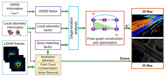
Figure 2.
Overview of the proposed mapping system. It combines navigation information from the GNSS, the wheel odometry, the IMU, and the LiDAR odometry. Degeneration analysis is performed for all these navigation sources. A pose graph is then constructed to calculate the optimal poses. The maps are then assembled based on the optimized poses.
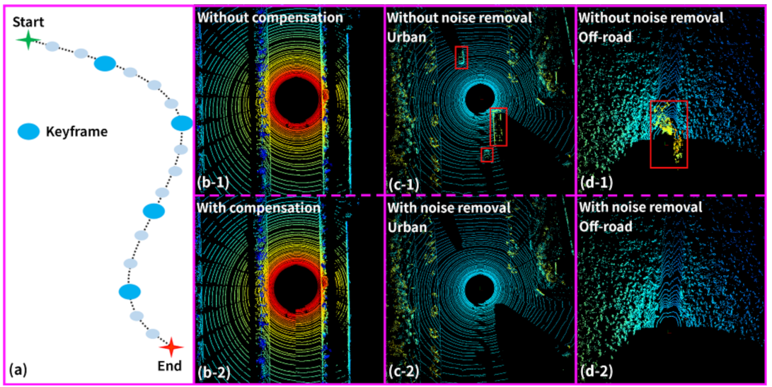
(I) Data preprocessing. This module is to preprocess the LiDAR point cloud, as shown in Figure 3. It includes three parts: keyframe selection, intra-frame compensation, and noise removal. Keyframes are selected based on the minimum odometric displacement (we set 1.0 m translation or 10 degree rotation). Distortion caused by LiDAR ego-motion is compensated through IMU/wheel encoder outputs [34,35]. We consider the moving objects as noise to the mapping system. They are filtered out by a multi-object detection and tracking method [36,37,38], as shown in Figure 3c. In the off-road environment, there might be floating dust as the wind blows, as shown in Figure 3d. These floating dust particles are removed by a specifically designed algorithm [39].
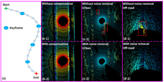
Figure 3.
The LiDAR data preprocessing includes three parts: the keyframe selection (a), the intra-frame compensation (b), and the noise removal (c,d). The noise either refers to the moving objects in the urban environment or the floating dust in the off-road environment.
(II) Factor graph-based pose optimization. As the core of the mapping system, a factor graph is then constructed to fuse the different kinds of navigation information. The factor graph consists of nodes and edges. Each node represents the pose of the keyframe to be estimated. The edges represent different kinds of constraints posed on the nodes. These include the GNSS factor produced by the GNSS information; the local odometry factor produced by the wheel odometer and IMU, and the scan matching factor generated by the preprocessed LiDAR scans. For each kind of factor, we need to set an appropriate information matrix for it, which represents its uncertainty. Estimating the uncertainty of each navigation source is one of the main contributions of this paper and will be described in the following subsections.
(III) Map construction and extension. The factor graph is then optimized using any off-the-shelf optimizers, including g2o, GTSAM, Ceres, etc. In this paper, we choose to use iSAM [13] as the optimizer. The optimized poses are then utilized to merge the keyframe point clouds into a consistent map. To ensure the scalability and the possible extension of the constructed map, we also design specific algorithms in Section 3.5.
3.2. Pose Graph Optimization
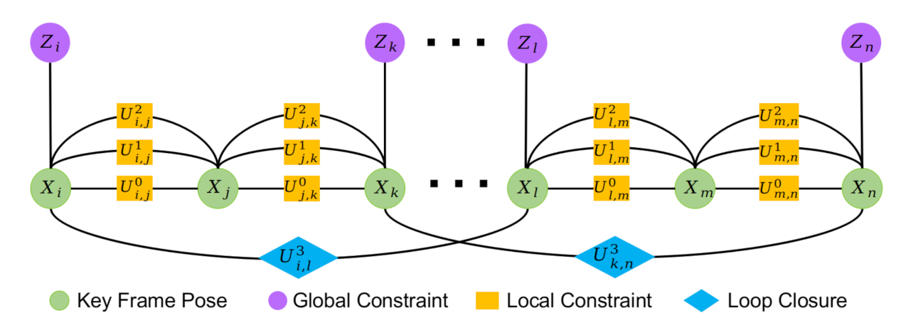
The pose graph that we constructed is shown in Figure 4. It integrates multiple sensor input data and outputs the optimized poses . Specifically, the following types of factors are involved: the motion prior factor from the IMU/wheel encoder [34,35], the scan-to-scan matching factor , the scan-to-submap matching factor , the loop closure factor , and the integrated GNSS/INS factor . For brevity, , , and are all named as the local constraints (as shown with orange squares in Figure 4).
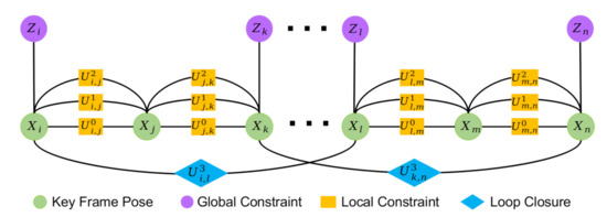
Figure 4.
Overview of the pose graph. There are mainly three types of factors: global constraints, local constraints, and loop closure constraints.
Based on Bayesian inference, the factor graph optimization is constructed as:
where X denotes the variable nodes, U represents the local constraints and loop closure constraints. Z denotes the GNSS/INS observations. As illustrated in [13], the motion model of can be described as:
where and denote the corresponding nodes connected by constraint , is the state transition process, is the process noise with covariance matrix , and is the constraint type. The observation model of can be expressed as:
where denotes the GNSS/INS observation over the node , is the observation function, and indicates the noise of the observation with covariance matrix .
We denote as . Then, and are the confidence matrices (also named information matrices), which reflect the reliability of the factors and can be calculated by the inverse of the standard deviation. To facilitate calculation, is usually represented as a diagonal matrix, which suggests that the six degrees of freedom of X (x, y, z, , , ) are independent of each other.
Quantitatively estimating the noise level of each factor is the key to improving the pose estimation accuracy. For the noise model of the IMU/wheel encoder factor, we use the approach proposed in [34]. The scan matching factor and the GNSS/INS factor are then analyzed as follows.
3.3. Scan Matching Factor
Mathematically, scan matching aims to estimate the relative transformation between the target point cloud and the reference point cloud . Based on the different types of , the scan matching factor involves three different forms: when is a neighboring keyframe, it forms a scan-to-scan matching factor; when represents a local sub-map, it generates a scan-to-submap matching factor. When is a scan of a revisited place, it generates a loop closure factor.
All three types of scan matching factors aim to minimize the following energy function:
where is a specifically designed energy function. This minimization function could be solved with the Levenberg–Marquardt algorithm through nonlinear iterations:
where and d is the residual error, which is usually represented as the geometric distance between two matching primitives.
It is noted in [31] that the eigenvalues of reflect the degeneracy state of the scan matching algorithm. Therefore, the authors of [31] defined the degeneration indicator as:
where is the smallest eigenvalue of . This method can detect degradation in some cases, but it might become unreliable, especially in the featureless off-road environment. Moreover, D has no probabilistic meanings, making it difficult to be integrated into the factor graph. To remedy this, we propose another degeneracy indicator in this paper. We firstly define as the update vector at each optimization iteration:
Then, by aggregating the from the last n iterations, we can calculate its covariance matrix:
Assuming that the six degrees of freedom are independent of each other, the diagonal matrix of is denoted as:
Intuitively, when the degeneration occurs, the corresponding elements of will increase. Therefore, we combine D with , and define its information matrix as:
where when ; otherwise, . is set to 300, and . is a normalization function. corresponds to the three types of scan matching constraints.
It is observed from Figure 4 that , , and are all used to calculate the local constraints between two neighboring keyframes. Among them, is directly obtainable from the hardware. is the most computationally expensive approach but provides the most accurate results in most circumstances. Generally, we have . Moreover, the proposed degeneration indicator could be applied to both and based on (11). When or degenerate, or will be automatically set to a lower value. has the lowest accuracy in most circumstances. When both and degenerate, will play a more important role.
For the loop closure constraint , it is usually more challenging than and due to the relatively large initial offset. Inspired by the work in [12], we adopt a combination of the global registration approach and the local registration approach, namely the CSM and LOAM. For LOAM, instead of performing the scan-to-scan registration or the scan-to-submap registration, we perform a submap-to-submap registration. Moreover, the degeneration analysis could also be applied to the local registration approach. Only those loop closure constraints with a low degeneration score are automatically added to the factor graph. For those possible degenerate loop closure candidates, either they are removed or a manual confirmation is performed.
3.4. GNSS/INS Factor
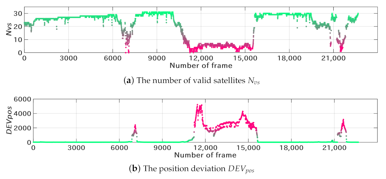
The integrated GNSS/INS device provides six-degrees-of-freedom global pose estimation over each node, which is expressed in (3). However, the GNSS signal might be blocked by tall buildings or trees, resulting in lower position accuracy. Besides the position output, the modern GNSS/INS devices also output affiliated information including the number of observed satellites , the position deviation , etc. Experimental results show that these values are strongly correlated with the GNSS/INS accuracy. Therefore, we use these values to adjust the information matrix in the factor graph. Let represent the information matrix of the GNSS/INS factor. It is a diagonal matrix and defined as:
where is set 10, and . is a normalization function. I is a diagonal matrix denoted as:
where is the translational weight factor and is the rotational weight factor. According to the units of the translation () and rotation () variables, we set .
3.5. Map Extension
The optimized poses are then used to stitch keyframes together to generate a global map. As shown in Figure 2, as the optimized poses are in 3D, we can generate both the 3D map and the 2D grayscale map. To facilitate the storage and the online usage of the map, the whole map is partitioned into small blocks by the global coordinate, and each small block is stored as a separate file. For the 3D map, each small block is stored using the Octree structure [40], whilst, for the 2D map, both the intensity and the height information are stored for each grid cell [6].
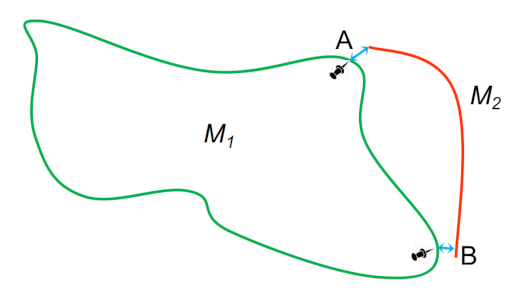
In general, maps cannot be built all at once and the map should be extendable to cover previously unseen areas. As an illustrative example shown in Figure 5, is a pre-built map, and is a new area that will be added to . To ensure the global consistency of the map, the following procedures are performed: (I) Generate the pose graph of and calculate the optimized poses of . (II) Find the keyframes in that are closest to , perform the submap-to-submap matching of these keyframes to , and obtain the relative poses of these keyframes against . (III) Assign high confidence to these optimized poses, and add them as extra constraints to the pose graph of . is then re-optimized and added to .
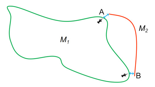
Figure 5.
An illustrative example of the map extension. The base map that has already been built is denoted as . represents the extended map. A and B represent two loop closure constraints that connect and .
4. Experimental Results
The experimental platforms are two modified self-driving vehicles shown in Figure 1. Each platform is equipped with a multi-channel LiDAR, an IMU, a wheel encoder, and a Novatel Propack 7 GNSS/INS system. Platform 2 is an industrial robot and the task loads have to be mounted on top of it. Therefore, the LiDAR has to be mounted in front of the vehicle and only has a limited FoV of around 200 degrees. The offline mapping system is run on a laptop with an Intel Core i7 CPU at 2.20 GHz.
4.1. Map Quality Assessment
To measure map quality and to facilitate quantitative comparisons of the results, the mean map entropy (MME) [41] is used. Given a map , the entropy of a point is calculated by:
where is the covariance matrix of the point set in a certain neighborhood of . The local radius is set to 0.5 m and is valid when the size of is larger than 5. The entropy is calculated for each point and the average is calculated as:
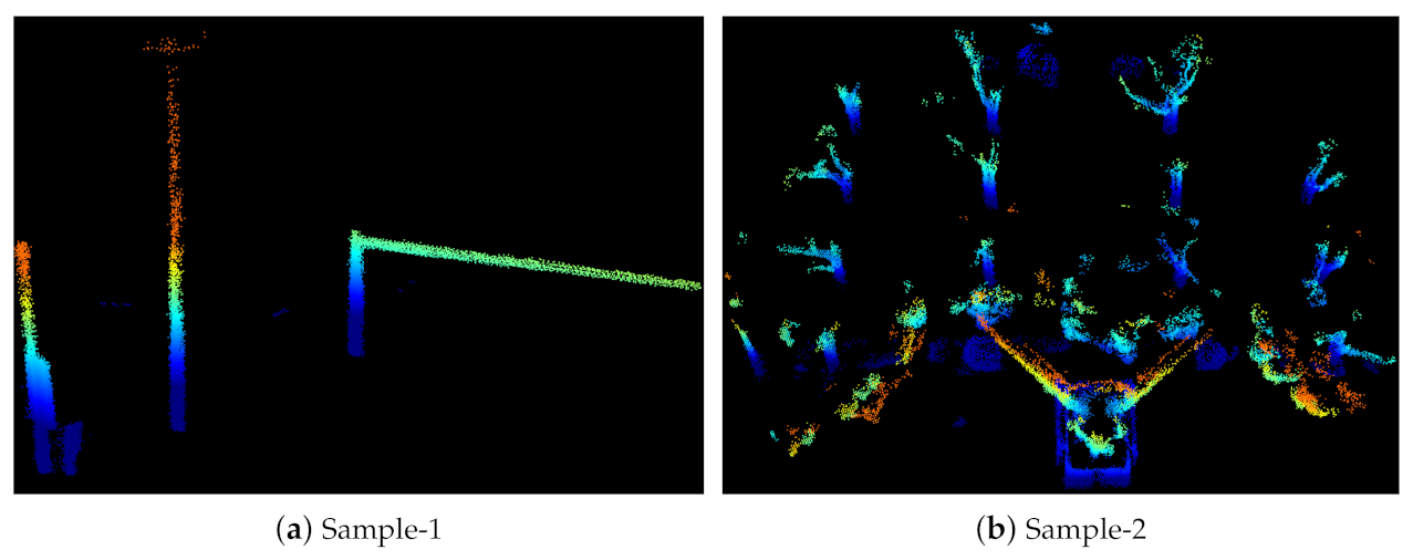
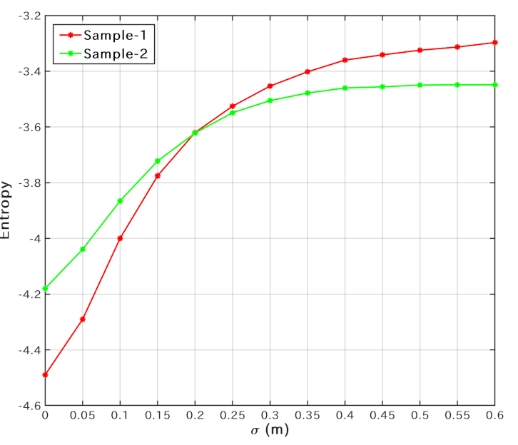
Generally, represents the sharpness of the map. Lower means higher map quality [41]. To verify the relationship between and the map quality, we add different levels of Gaussian noise (characterized by a standard deviation of ) to maps sampled from two scenes. The original maps with are shown in Figure 6. The resulting map entropy plotted against is shown in Figure 7. For both samples, is positively correlated with , indicating that higher entropy characterizes poorer map quality.
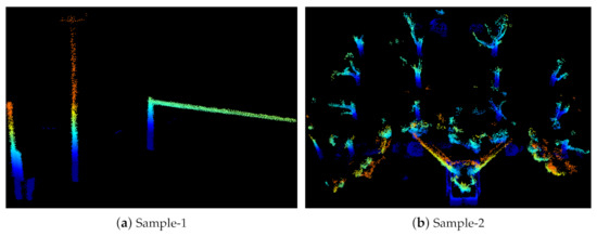
Figure 6.
Two samples for evaluating the mean map entropy. Sample-1 includes traffic signs and light poles. Sample-2 is mainly composed of trees, bushes, and a sculpture.
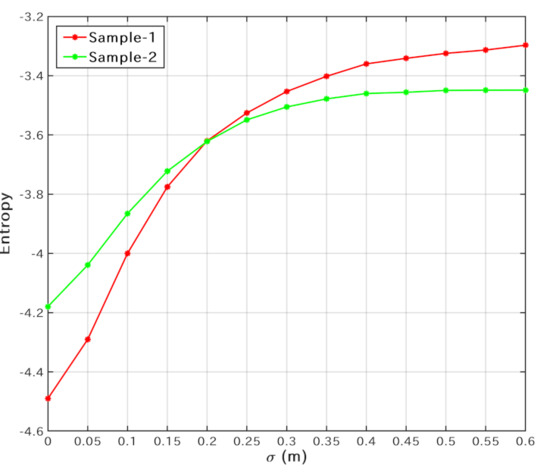
Figure 7.
The resulting map entropy against the standard deviation of Gaussian noise.
4.2. Results of Noise Removal
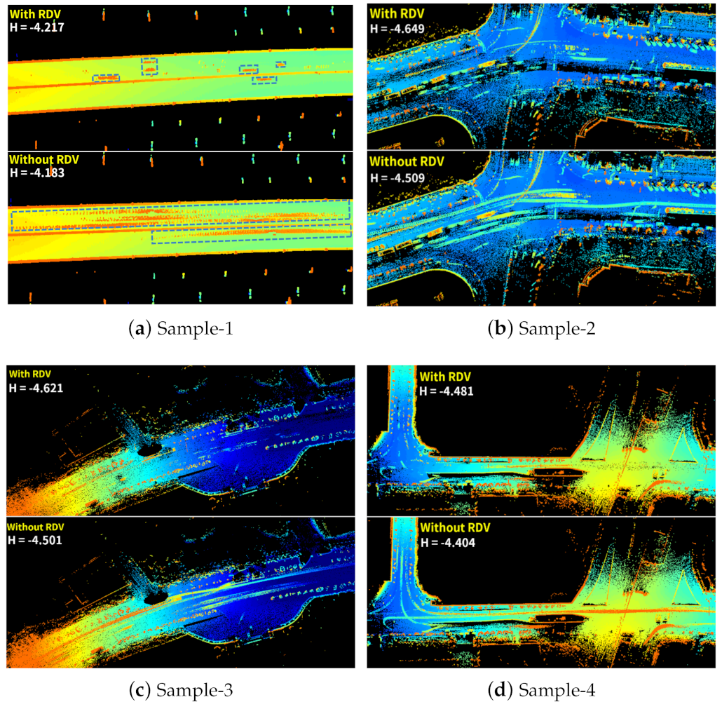
Removal of dynamic vehicles: The comparison results with and without the removal of dynamic vehicles (RDV) are shown in Figure 8. As shown in Figure 8, the ghost shadows caused by moving vehicles (highlighted with blue dotted boxes in Figure 8a) are mostly filtered out by the proposed mapping system. Furthermore, the decrease in after the removal of dynamic vehicles suggests that the map quality has been improved.
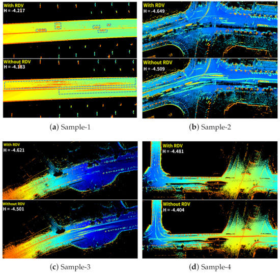
Figure 8.
Comparison of the mapping results and the MME values in four scenes with (top) and without (bottom) the removal of dynamic vehicles.
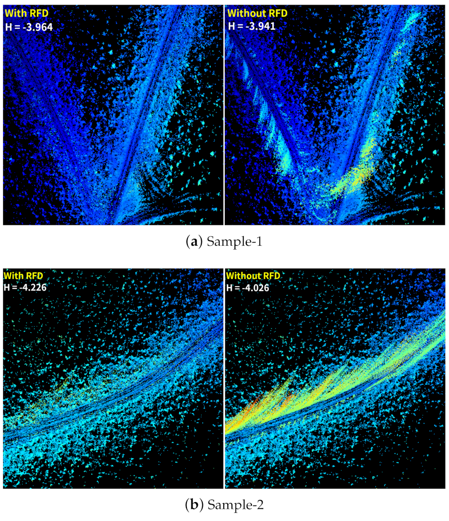
Removal of floating dust: Two comparative mapping results with and without the removal of floating dust (RFD) in off-road scenarios are shown in Figure 9. It is obvious that the map quality has been improved after the removal of floating dust.
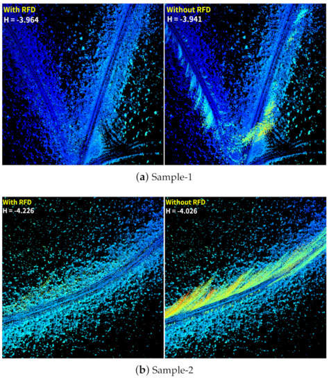
Figure 9.
The mapping results and the MME values with and without the removal of floating dust.
4.3. Analysis of Degeneracy-Aware Factors
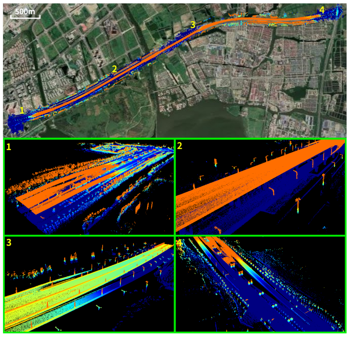
The degeneration analysis of the GNSS/INS factor and the scan matching factor is performed in this section. The first dataset was collected by Platform 1 in city environments with a total driving length of 19.3 km, as shown in Figure 10. The evaluation of the GNSS/INS status is shown in Figure 11. Intuitively, frames with lower or higher have worse GNSS/INS status. A manual confirmation indicates that these frames are mainly captured under high bridges.
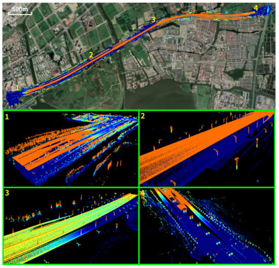
Figure 10.
The mapping results are overlaid on the satellite image. Four possible degenerate scenarios are shown at the bottom.

Figure 11.
Evaluation of the GNSS/INS status. Frames with well-conditioned GNSS/INS status are highlighted in green.
For the scan matching degeneration analysis, we evaluate the degeneracy indicators D and . For easy comparison with D, we define E based on :
where and are scale factors. The values of D and E are calculated for each scan-to-scan and scan-to-submap registration, and the results are shown in Figure 12a–d. Frames with lower D or higher E are more prone to degeneration and they are highlighted in pink. These frames are mostly captured on the highway, with less geometrical structures, or surrounded by many vehicles, as shown in sub-figures 2 and 3 in Figure 10. Furthermore, the scan-to-submap matching constraints have larger D and smaller E than the scan-to-scan matching constraints. Therefore, the scan-to-scan matching constraints are generally more prone to degeneration than the scan-to-submap constraints.
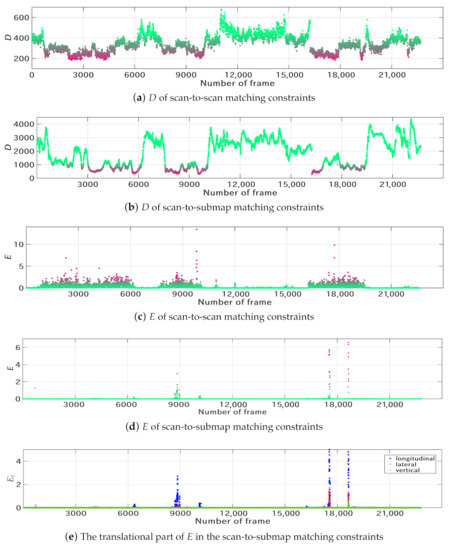
Figure 12.
Degeneracy indicators of the scan matching constraints. In (a–d), the non-degenerate cases are shown in green. Frames with lower D or higher E are more prone to degeneration (shown in pink). The translation components of of the scan-to-submap matching constraints are shown in (e).
Moreover, the degeneration direction can also be inferred from the six components of . Figure 12e shows the translational components of for the scan-to-submap matching constraints. It is observed that the longitudinal direction is more prone to degeneration, as shown by the blue dots. This is consistent with the feature distribution shown in close views 2 and 3 of Figure 10, where repeated features mostly appear along the longitudinal direction.
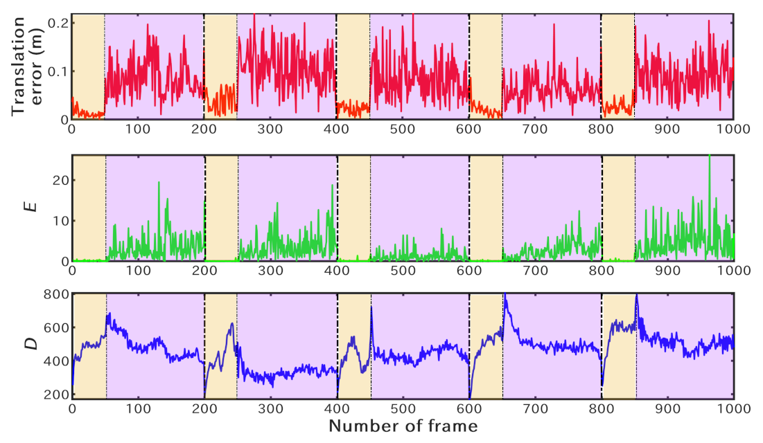
To further compare the performance of E and D, we conducted a test on the dataset collected by Platform 2 in the off-road scenario. We randomly selected five sets of data, each of which contained 200 keyframes. Zero-mean Gaussian noise was added to the last 150 scans for each set of data. Then, the scan matching algorithm was performed to compute the relative transformation between every two keyframes. We evaluated the translation errors and the degeneration indicators of the scan-to-submap matching factors. In Figure 13, the non-degenerate cases (without Gaussian noise) are shown in yellow and the degenerate cases (with Gaussian noise) are shown in pink. The translation error (shown in red) increases significantly for the last 150 keyframes of each group. Furthermore, the proposed degeneration indicator E (shown in green) shows a similar trend to the translation error, exhibiting better performance than the degeneration indicator D (shown in blue). Further comparison results between D and E will be described in Section 4.4.
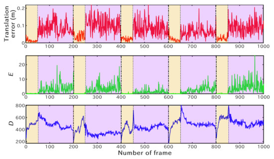
Figure 13.
Comparison results of the degeneration indicators. Five groups with a total of 1000 keyframes are tested. Gaussian noise is added to generate the degraded cases (marked in pink). The translation errors of the scan-to-submap matching constraints are shown in red. The degeneration indicators E and D are shown in green and blue, respectively.
4.4. Analysis of Loop Closures
In most scenarios, the GNSS/INS can provide a good initial value for loop closure detection. In the case of GNSS signal blockage, the loop closure has to be detected by the scan matching algorithm. In the featureless off-road environment, loop closure detection becomes more challenging.
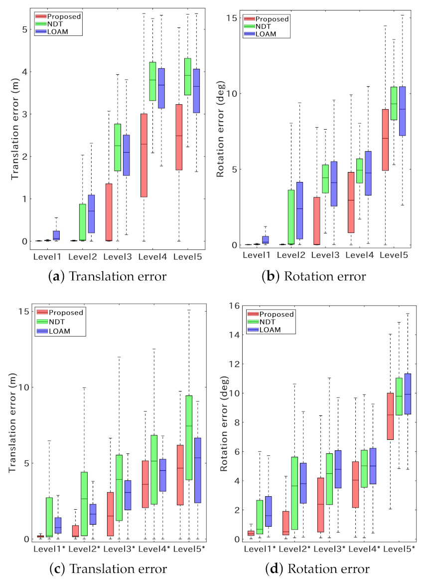
We collected three sets of data by Platform 2 in the off-road scenario. A total of 846 pairs of loop closure constraints were generated, including 423 pairs with small translational offsets (around 2 m) and 423 pairs with large offsets (around 15 m). Similar to [12], the ground-truth position of each keyframe was obtained using the graph SLAM algorithm. For each group, we added five levels of translational and rotational noise, obtaining a total number of 4230 loop closure pairs. The noise parameters are shown in Table 1. The number shown in this table represents the mean () of the added Gaussian noise and the standard deviation () is set to of .

Table 1.
Five levels of noise for loop closure registration.
We choose NDT and LOAM as the baseline approaches. Figure 14 shows the error statistics of loop closure registration. Overall, the proposed method obtains the best performance at all levels of difficulty for both two groups. Furthermore, Figure 15 shows the proportion of correct loop closure registrations. We compare the registration result with the ground truth. It is considered as a correct registration if the translation error is less than 0.2 m and the rotation error is less than 0.5 degrees. Based on Figure 14 and Figure 15, the proposed approach performs best in both the overall accuracy and the success rate.

Figure 14.
Boxplots of the registration error of the loop closure constraints. The box spans the first and third quartiles. (a,b) show the results of group one with small offsets. (c,d) show the results of group two with large offsets.

Figure 15.
Proportion of the correct loop closures obtained by three approaches. (a) shows the results of group one with small offsets, and (b) shows the results of group two with large offsets.
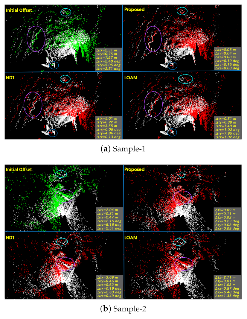
Two typical loop closure matching results are shown in Figure 16. The large position offset and the limited FoV of each LiDAR frame pose significant challenges to the loop closure registration algorithm. It is observed in Figure 16 that both NDT and LOAM failed to obtain the correct registration result. In contrast, the proposed approach uses a combination of the global registration approach (CSM) and local registration approach (LOAM-based submap-to-submap matching) and correctly computed the registration results.
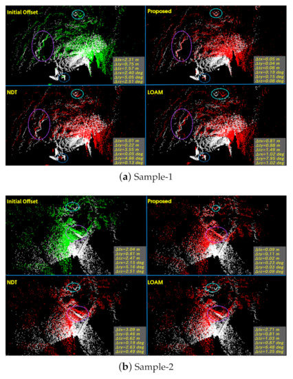
Figure 16.
Two typical loop closure matching results. The target scan is shown in white, the original source scan is shown in green, and the transformed source scan is shown in red. The registration errors are presented and some comparable details are marked by ellipses.
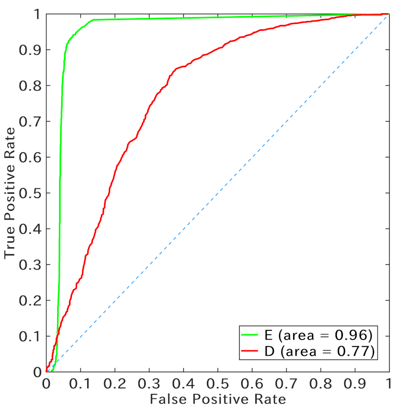
Moreover, the proposed degeneracy indicator E (simplified from (16)) is also evaluated for the loop closure registration algorithm. The performance of E and D is shown in Figure 17. The ROC curves are obtained by evaluating 4230 pairs of loop closures. The proposed indicator E obtains much better performance than the indicator D.

Figure 17.
ROC curves for the degeneracy indicators E and D. This evaluation is performed using a total of 4230 pairs of loop closures, including 2031 positive (matching) pairs and 2199 negative (non-matching) pairs.
4.5. Mapping Results
In addition to the mapping results described in Section 4.3, the proposed mapping system is also tested under several other challenging scenarios.
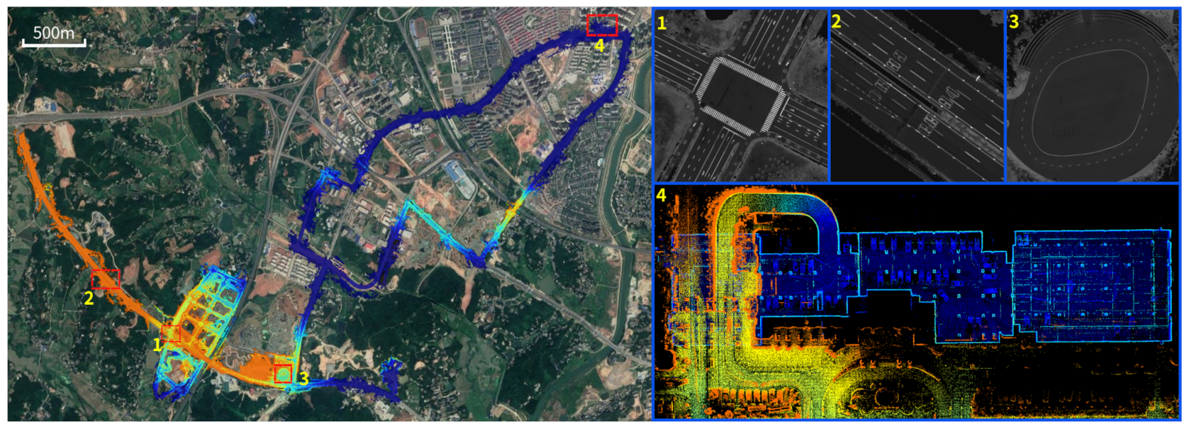
Mapping results in challenging city scenarios: The mapping system is tested in a complex city scenario, including the city road under a bridge, highways, and an underground parking garage, as shown in Figure 18. Moreover, the data were collected during a high-traffic period, when the vehicle was always surrounded by many other moving objects. It is observed that the lane markings on the ground are clearly visible in the enlarged 2D grayscale maps (as shown in close views 1–3 of Figure 18). The high-precision 3D point cloud map of the underground parking garage suggests that the mapping system could accurately map the area without the GNSS signal, and the built map could be seamlessly aligned to the area with the GNSS signal.
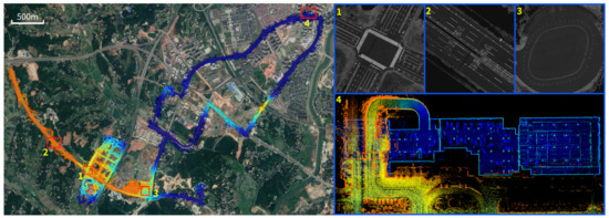
Figure 18.
Mapping results in challenging city scenarios. The map is overlaid on the satellite image. Four close views labeled 1–4 are shown on the right. Sub-figures 1–3 show the reflectance intensity map. The 3D map of an underground parking lot is shown in sub-figure 4.
The computational efficiency of the mapping system is also evaluated. In this test, the scan matching and the removal of dynamic objects can be processed in parallel at a frequency of 10 Hz. The route is around 34.5 km and consists of 31,189 keyframes. The detection and verification of loop closures take less than 15 min and the optimization can be performed in a few seconds. Finally, the rendering of maps takes around 20 min at a frequency of around 30 Hz. Overall, the construction of the map takes less than 90 min on a single CPU.
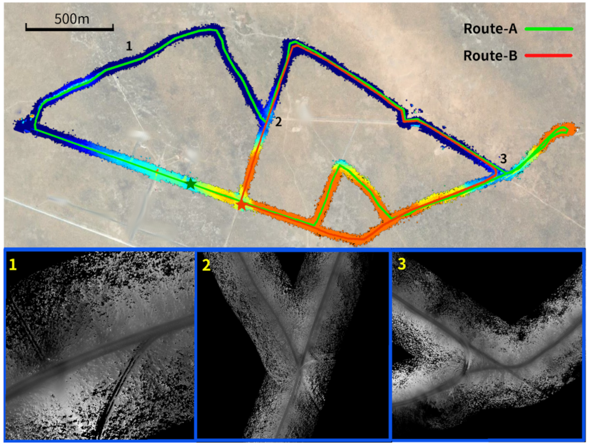
Mapping results in off-road scenarios:Figure 19 shows the mapping results tested on Platform 2 in the featureless off-road scenarios. Two sets of data with a total driving length of 10.859 km were collected. The driving route and the generated 3D map are overlaid on the satellite image. Three enlarged grayscale maps shown at the bottom of Figure 19 prove the effectiveness of the mapping system in the featureless off-road environment even with a LiDAR with limited FoV.

Figure 19.
Mapping results in off-road scenarios. Data were collected along two routes. The complete map overlaid on the satellite image is shown at the top. Three zoom-in views labeled 1–3 are shown at the bottom, where the grey value encodes the height information.
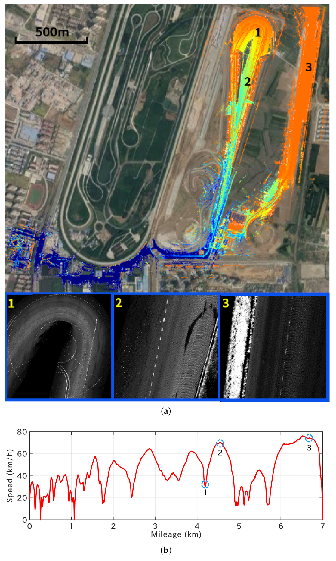
Mapping results at a high driving speed: In all the above experiments, the vehicle drives at a speed of around 30 km/h. In this test, we evaluate the mapping system at a higher driving speed. The mapping results are shown in Figure 20a. Some of the scenarios are relatively open with fewer feature points. The vehicle drives at an average speed of 38.2 km/h, and the maximum speed reaches 76.2 km/h (as shown in Figure 20b). Some of the mapping results are shown at the bottom of Figure 20a, where the lane markings on the ground are visible, demonstrating the effectiveness of the mapping system.

Figure 20.
Mapping results at a higher driving speed. Three zoom-in views of the corresponding 2D grayscale maps (rendered by the reflectance intensity values) are shown at the bottom in (a). The driving speed is shown in (b).
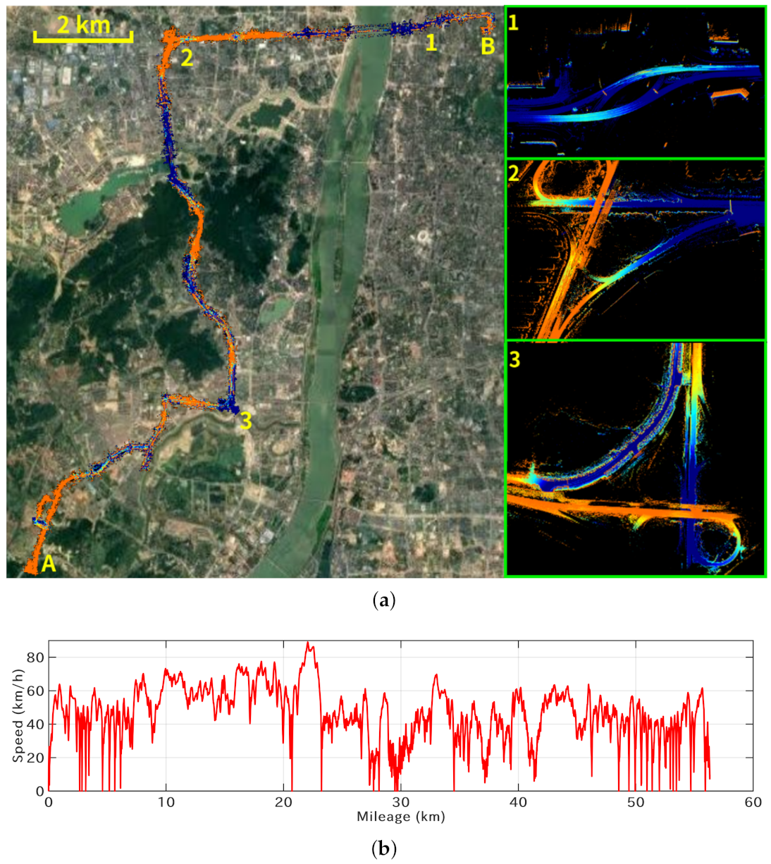
Large-scale mapping: Finally, the mapping system was also tested in a large-scale highly dynamic urban scenario. As shown in Figure 21, two sets of data were collected. The first dataset was collected from A to B on 3 September 2019 and the second dataset was collected from B to A on 28 July 2020. The total driving length is 56.3 km and the driving speed is shown in Figure 21b. A large number of dynamic vehicles make the scan matching tend to degenerate, especially over the high bridges. Moreover, GNSS signal blockage frequently occurs due to tall buildings. These problems are handled well by the degeneration analysis proposed in this paper.
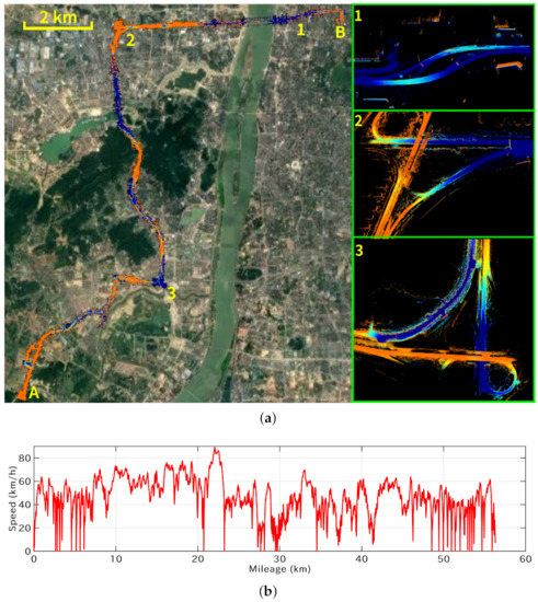
Figure 21.
Mapping results in large-scale settings. The total driving length is 56.3 km and the maximum elevation change is 37.2 m. The constructed 3D map overlaid on the satellite image is shown in (a). Three enlarged views are shown on the right. The driving speed is shown in (b) with a maximum speed of 88.92 km/h.
5. Conclusions
In this paper, we proposed a framework for LiDAR-based 3D mapping in challenging scenarios. A degeneracy-aware factor graph is constructed by fusing different kinds of navigation information to improve the mapping accuracy and robustness. The reliability of each factor is analyzed, and the degeneration state can be effectively detected. A new scan matching degeneracy indicator is proposed. This new indicator can be seamlessly integrated into the pose graph optimization framework. The loop closure constraint can be reliably estimated by an improved submap-to-submap matching method even with a large initial position offset or a limited overlap field of view. Extensive experiments in several challenging scenarios are performed. Results indicate that the proposed mapping system works well both in the highly dynamic urban scenarios and the featureless off-road scenarios, even with GNSS signal blockage or at a higher driving speed. In the future, we plan to augment the mapping system with more informative visual features captured from cameras.
Author Contributions
Conceptualization, R.R., H.F. and Z.S.; methodology, R.R., H.F. and H.X.; software, R.R., H.F. and H.X.; validation, R.R.; formal analysis, Z.S.; investigation, R.R.; resources, Z.S., K.D. and P.W.; data curation, R.R., H.F. and H.X.; writing—original draft preparation, R.R.; writing—review and editing, R.R. and H.F.; visualization, R.R.; supervision, Z.S., K.D. and P.W.; project administration, H.F. and Z.S.; funding acquisition, Z.S., K.D. and P.W. All authors have read and agreed to the published version of the manuscript.
Funding
This research was funded by the National Natural Science Foundation of China under No.61790565, the Natural Science Foundation of Hunan Province of China under Grant 2019JJ50738, the Foundation of Science and Technology on Near-Surface Detection Laboratory under No.6142414180207, and pre-research project 060601 of the Manned Space Flight.
Institutional Review Board Statement
Not applicable.
Informed Consent Statement
Not applicable.
Data Availability Statement
Data sharing not applicable.
Conflicts of Interest
The authors declare no conflict of interest.
References
- Cadena, C.; Carlone, L.; Carrillo, H.; Latif, Y.; Scaramuzza, D.; Neira, J.; Reid, I.; Leonard, J.J. Past, present, and future of simultaneous localization and mapping: Toward the robust-perception age. IEEE Trans. Robot. 2016, 32, 1309–1332. [Google Scholar] [CrossRef]
- Yang, S.; Zhu, X.; Nian, X.; Feng, L.; Qu, X.; Ma, T. A robust pose graph approach for city scale LiDAR mapping. In Proceedings of the IEEE/RSJ International Conference on Intelligent Robots and Systems (IROS 2018), Madrid, Spain, 1–5 October 2018; pp. 1175–1182. [Google Scholar]
- Ilçi, V.; Toth, C.K. High Definition 3D Map Creation Using GNSS/IMU/LiDAR Sensor Integration to Support Autonomous Vehicle Navigation. Sensors 2020, 20, 899. [Google Scholar] [CrossRef] [PubMed]
- Hirabayashi, M.; Sujiwo, A.; Monrroy, A.; Kato, S.; Edahiro, M. Traffic light recognition using high-definition map features. Robot. Auton. Syst. 2019, 111, 62–72. [Google Scholar] [CrossRef]
- Li, Q.; Queralta, J.P.; Gia, T.N.; Zou, Z.; Westerlund, T. Multi-Sensor Fusion for Navigation and Mapping in Autonomous Vehicles: Accurate Localization in Urban Environments. Unmanned Syst. 2020, 8, 229–237. [Google Scholar] [CrossRef]
- Fu, H.; Yu, R.; Ye, L.; Wu, T.; Xu, X. An Efficient Scan-to-Map Matching Approach Based on Multi-channel Lidar. J. Intell. Robot. Syst. 2018, 91, 501–513. [Google Scholar] [CrossRef]
- Zheng, L.; Zhu, Y.; Xue, B.; Liu, M.; Fan, R. Low-Cost GPS-Aided LiDAR State Estimation and Map Building. In Proceedings of the IEEE International Conference on Imaging Systems and Techniques (IST 2019), Abu Dhabi, United Arab Emirates, 9–10 December 2019; pp. 1–6. [Google Scholar]
- Kühner, T.; Kümmerle, J. Large-Scale Volumetric Scene Reconstruction using LiDAR. In Proceedings of the IEEE International Conference on Robotics and Automation (ICRA 2020), Paris, France, 31 May–31 August 2020; pp. 6261–6267. [Google Scholar]
- Zhang, J.; Singh, S. Laser-visual-inertial odometry and mapping with high robustness and low drift. J. Field Robot. 2018, 35, 1242–1264. [Google Scholar] [CrossRef]
- Maaref, M.; Kassas, Z.M. Ground Vehicle Navigation in GNSS-Challenged Environments Using Signals of Opportunity and a Closed-Loop Map-Matching Approach. IEEE Trans. Intell. Transp. Syst. 2020, 21, 2723–2738. [Google Scholar] [CrossRef]
- Kubelka, V.; Oswald, L.; Pomerleau, F.; Colas, F.; Svoboda, T.; Reinstein, M. Robust Data Fusion of Multimodal Sensory Information for Mobile Robots. J. Field Robot. 2015, 32, 447–473. [Google Scholar] [CrossRef]
- Fu, H.; Yu, R. LIDAR Scan Matching in Off-Road Environments. Robotics 2020, 9, 35. [Google Scholar] [CrossRef]
- Kaess, M.; Ranganathan, A.; Dellaert, F. iSAM: Incremental Smoothing and Mapping. IEEE Trans. Robot. 2008, 24, 1365–1378. [Google Scholar] [CrossRef]
- He, G.; Yuan, X.; Zhuang, Y.; Hu, H. An Integrated GNSS/LiDAR-SLAM Pose Estimation Framework for Large-Scale Map Building in Partially GNSS-Denied Environments. IEEE Trans. Instrum. Meas. 2021, 70, 1–9. [Google Scholar]
- Pomerleau, F.; Colas, F.; Siegwart, R.; Magnenat, S. Comparing ICP variants on real-world data sets - Open-source library and experimental protocol. Auton. Robot. 2013, 34, 133–148. [Google Scholar] [CrossRef]
- Segal, A.; Hähnel, D.; Thrun, S. Generalized-ICP. In Proceedings of the Robotics: Science and Systems V, Seattle, WA, USA, 28 June–1 July 2009. [Google Scholar]
- Magnusson, M.; Lilienthal, A.J.; Duckett, T. Scan registration for autonomous mining vehicles using 3D-NDT. J. Field Robot. 2007, 24, 803–827. [Google Scholar] [CrossRef]
- Zhang, J.; Singh, S. LOAM: Lidar Odometry and Mapping in Real-time. In Proceedings of the Robotics: Science and Systems X, Berkeley, CA, USA, 12–16 July 2014. [Google Scholar]
- Olson, E.B. Real-time correlative scan matching. In Proceedings of the IEEE International Conference on Robotics and Automation (ICRA 2009), Kobe, Japan, 12–17 May 2009; pp. 4387–4393. [Google Scholar]
- Hess, W.; Kohler, D.; Rapp, H.; Andor, D. Real-time loop closure in 2D LIDAR SLAM. In Proceedings of the IEEE International Conference on Robotics and Automation (ICRA 2016), Stockholm, Sweden, 16–21 May 2016; pp. 1271–1278. [Google Scholar]
- Ren, R.; Fu, H.; Wu, M. Large-Scale Outdoor SLAM Based on 2D Lidar. Electronics 2019, 8, 613. [Google Scholar] [CrossRef]
- Dubé, R.; Dugas, D.; Stumm, E.; Nieto, J.I.; Siegwart, R.; Cadena, C. SegMatch: Segment based place recognition in 3D point clouds. In Proceedings of the IEEE International Conference on Robotics and Automation (ICRA 2017), Singapore, 29 May–3 June 2017; pp. 5266–5272. [Google Scholar]
- Milioto, A.; Vizzo, I.; Behley, J.; Stachniss, C. RangeNet ++: Fast and Accurate LiDAR Semantic Segmentation. In Proceedings of the IEEE/RSJ International Conference on Intelligent Robots and Systems (IROS 2019), Macau, China, 3–8 November 2019; pp. 4213–4220. [Google Scholar]
- Kong, X.; Yang, X.; Zhai, G.; Zhao, X.; Zeng, X.; Wang, M.; Liu, Y.; Li, W.; Wen, F. Semantic Graph Based Place Recognition for 3D Point Clouds. In Proceedings of the IEEE/RSJ International Conference on Intelligent Robots and Systems (IROS 2020), Las Vegas, NV, USA, 24 October–24 January 2021; pp. 8216–8223. [Google Scholar]
- Kümmerle, R.; Grisetti, G.; Strasdat, H.; Konolige, K.; Burgard, W. G2o: A general framework for graph optimization. In Proceedings of the IEEE International Conference on Robotics and Automation (ICRA 2011), Shanghai, China, 9–13 May 2011; pp. 3607–3613. [Google Scholar]
- Kaess, M.; Johannsson, H.; Roberts, R.; Ila, V.; Leonard, J.J.; Dellaert, F. iSAM2: Incremental smoothing and mapping with fluid relinearization and incremental variable reordering. In Proceedings of the IEEE International Conference on Robotics and Automation (ICRA 2011), Shanghai, China, 9–13 May 2011; pp. 3281–3288. [Google Scholar]
- Agarwal, S.; Mierle, K. Ceres solver: Tutorial & reference. Google Inc. 2012, 2, 72. [Google Scholar]
- Sünderhauf, N.; Protzel, P. Towards a robust back-end for pose graph SLAM. In Proceedings of the IEEE International Conference on Robotics and Automation (ICRA 2012), St. Paul, MN, USA, 14–18 May 2012; pp. 1254–1261. [Google Scholar]
- Olson, E.; Agarwal, P. Inference on networks of mixtures for robust robot mapping. Int. J. Robot. Res. 2013, 32, 826–840. [Google Scholar] [CrossRef]
- Bonnabel, S.; Barczyk, M.; Goulette, F. On the covariance of ICP-based scan-matching techniques. In Proceedings of the IEEE American Control Conference (ACC 2016), Boston, MA, USA, 6–8 July 2016; pp. 5498–5503. [Google Scholar]
- Zhang, J.; Kaess, M.; Singh, S. On degeneracy of optimization-based state estimation problems. In Proceedings of the IEEE International Conference on Robotics and Automation (ICRA 2016), Stockholm, Sweden, 16–21 May 2016; pp. 809–816. [Google Scholar]
- Aldera, R.; Martini, D.D.; Gadd, M.; Newman, P. What Could Go Wrong? In Introspective Radar Odometry in Challenging Environments. In Proceedings of the IEEE Intelligent Transportation Systems Conference (ITSC 2019), Auckland, New Zealand, 27–30 October 2019; pp. 2835–2842. [Google Scholar]
- Ju, X.; Xu, D.; Zhao, X.; Yao, W.; Zhao, H. Learning Scene Adaptive Covariance Error Model of LiDAR Scan Matching for Fusion Based Localization. In Proceedings of the IEEE Intelligent Vehicles Symposium (IV 2019), Paris, France, 9–12 June 2019; pp. 1789–1796. [Google Scholar]
- Xue, H.; Fu, H.; Dai, B. IMU-Aided High-Frequency Lidar Odometry for Autonomous Driving. Appl. Sci. 2019, 9, 1506. [Google Scholar] [CrossRef]
- Lin, J.; Zhang, F. Loam livox: A fast, robust, high-precision LiDAR odometry and mapping package for LiDARs of small FoV. In Proceedings of the IEEE International Conference on Robotics and Automation (ICRA 2020), Paris, France, 31 May–31 August 2020; pp. 3126–3131. [Google Scholar]
- Chen, T.; Wang, R.; Dai, B.; Liu, D.; Song, J. Likelihood-Field-Model-Based Dynamic Vehicle Detection and Tracking for Self-Driving. IEEE Trans. Intell. Transp. Syst. 2016, 17, 3142–3158. [Google Scholar] [CrossRef]
- Ren, R.; Fu, H.; Hu, X.; Xue, H.; Li, X.; Wu, M. Towards Efficient and Robust LiDAR-based 3D Mapping in Urban Environments. In Proceedings of the IEEE International Conference on Unmanned Systems (ICUS 2020), Harbin, China, 27–28 November 2020; pp. 511–516. [Google Scholar]
- Pagad, S.; Agarwal, D.; Narayanan, S.; Rangan, K.; Kim, H.; Yalla, V.G. Robust Method for Removing Dynamic Objects from Point Clouds. In Proceedings of the IEEE International Conference on Robotics and Automation (ICRA 2020), Paris, France, 31 May–31 August 2020; pp. 10765–10771. [Google Scholar]
- Fu, H.; Xue, H.; Ren, R. Fast Implementation of 3D Occupancy Grid for Autonomous Driving. In Proceedings of the IEEE International Conference on Intelligent Human-Machine Systems and Cybernetics (IHMSC 2020), Hangzhou, China, 22–23 August 2020; Volume 2, pp. 217–220. [Google Scholar]
- Hornung, A.; Wurm, K.M.; Bennewitz, M.; Stachniss, C.; Burgard, W. OctoMap: An efficient probabilistic 3D mapping framework based on octrees. Auton. Robot. 2013, 34, 189–206. [Google Scholar] [CrossRef]
- Droeschel, D.; Behnke, S. Efficient Continuous-Time SLAM for 3D Lidar-Based Online Mapping. In Proceedings of the IEEE International Conference on Robotics and Automation (ICRA 2018), Brisbane, Australia, 21–25 May 2018; pp. 1–9. [Google Scholar]
Publisher’s Note: MDPI stays neutral with regard to jurisdictional claims in published maps and institutional affiliations. |
© 2021 by the authors. Licensee MDPI, Basel, Switzerland. This article is an open access article distributed under the terms and conditions of the Creative Commons Attribution (CC BY) license (https://creativecommons.org/licenses/by/4.0/).


