Abstract
Satellite-retrieved aerosol optical depth (AOD) data are extensively integrated with ground-level measurements to achieve spatially continuous fine particulate matters (PM2.5). Current satellite-based methods however face challenges in obtaining highly accurate and reasonable PM2.5 distributions due to the inability to handle both spatial non-stationarity and complex non-linearity in the PM2.5–AOD relationship. High-resolution (<1 km) PM2.5 products over the whole of China for fine exposure assessment and health research are also lacking. This study aimed to predict 750 m resolution ground-level PM2.5 in China with the high-resolution Visible Infrared Imaging Radiometer Suite (VIIRS) intermediate product (IP) AOD data using a newly developed geographically neural network weighted regression (GNNWR) model. The performance evaluations demonstrated that GNNWR achieved higher prediction accuracy than the widely used methods with cross-validation and predictive R2 of 0.86 and 0.85. Satellite-derived monthly 750 m resolution PM2.5 data in China were generated with robust prediction accuracy and almost complete coverage. The PM2.5 pollution was found to be greatly improved in 2018 in China with annual mean concentration of 31.07 ± 17.52 µg/m3. Nonetheless, fine-scale PM2.5 exposures at multiple administrative levels suggested that PM2.5 pollution in most urban areas needed further control, especially in southern Hebei Province. This work is the first to evaluate the potential of VIIRS IP AOD in modeling high-resolution PM2.5 over large-scale. The newly satellite-derived PM2.5 data with high spatial resolution and high prediction accuracy at the national scale are valuable to advance environmental and health researches in China.
1. Introduction
Fine particulate matters (e.g., PM2.5 with aerodynamic diameter below 2.5 μm) are directly adverse to the environment and human health [1,2]. With the continued development of the economy and industry in recent decades, China is currently experiencing heavily PM2.5 pollutions due to the mass emissions of air pollutants [3,4,5]. The ground-level monitoring network built in China supplies precise and stable observations, but limitations are inevitably encountered in evaluating pollution exposures and health effects due to the uneven and sparse measurements [6,7]. It is crucial to portray the complete space-time distributions of PM2.5 to facilitate environmental and health researches in China.
Unlike ground-level measurements, satellite-based derivatives provide wide coverage datasets. Considering the significant correlation between PM2.5 and aerosol optical depth (AOD), numerous studies have integrated satellite-retrieved AOD to map surface PM2.5 concentrations [7,8,9,10,11,12,13,14]. High-resolution satellite-retrieved AOD datasets are conducive to reveal detailed PM2.5 pollutions and benefit fine-scale researches. These accessible high-resolution (≤3 km) AOD products used in PM2.5 modeling mainly include 3 km Moderate Resolution Imaging Spectroradiometer (MODIS) AOD [15,16], 1 km Multi-Angle Implementation of Atmospheric Correction (MAIAC) AOD [13,14,17,18], and 750 m Visible Infrared Imaging Radiometer Suite (VIIRS) intermediate product (IP) AOD [19,20]. The data quality of VIIRS IP AOD have been fully verified by comparing with various satellite-based AOD datasets and the Aerosol Robotic Network (AERONET) [15,21,22,23]. Although its accuracy is somehow inferior to other widely used AOD products, the VIIRS IP AOD with unprecedented high-resolution is believed to have the potential to further enhance exposure assessments and pollution researches on fine-scale [20]. Nevertheless, its ability to estimate PM2.5 has only been evaluated in limited studies and its capacity of PM2.5 modeling over large-scale with complex dispersions has not been explored.
On the other hand, many statistical models are established to illustrate the relationship between PM2.5 and AOD (denoted as PM2.5–AOD) and spatially continuous PM2.5 concentrations are reconstructed with almost equivalent or superior accuracy compared to conventional simulation-based methods. Ordinary linear regression (OLR) was conducted by incorporating satellite-retrieved AOD and obtained acceptable PM2.5 estimates in various study areas [24,25]. Considering the spatial non-stationarity in the PM2.5–AOD relationship, geographically weighted regression (GWR) using local spatial regression was applied and achieved fairly reasonable results [6,26,27,28,29]. Although GWR can depict simple non-linear spatial relationship, PM2.5–AOD modeling is recognized as a complex non-linear multivariate problem due to its diverse dispersion mechanisms [30,31]. Artificial neural network (ANN) algorithms were subsequently implemented to accurately map PM2.5 concentrations and outperformed classical statistical methods [31,32,33,34,35,36]. Due to the easily local converge of the well-known back-propagation neural network, the general regression neural network (GRNN) with self-organizing and adaptive function was introduced to estimate PM2.5 and showed decent prediction accuracy [37,38,39]. ANNs have been increasingly confirmed to successfully address the complex non-linearity in PM2.5 modeling, but their spatial predictions may exhibit unreasonable patterns and their established relationships are spatially uninterpretable [40]. It is increasingly urgent to develop new models to deal with both spatial non-stationarity and complex non-linearity in the PM2.5–AOD relationship to achieve highly accurate and reasonable PM2.5 distributions.
In the meantime, many researchers have applied diverse satellite-retrieved AOD and PM2.5–AOD models to generate spatially continuous PM2.5 in China at both regional and national scales [6,7,14,16,17,26,39,41,42]. However, the PM2.5–AOD relationship across China is significantly complicated due to its complicated environmental variability and wide geographical range. It is still challenging to predict highly accurate and reasonable high-resolution (<1 km) PM2.5 across the entire China. In view of this, this study aims to estimate 750 m resolution surface PM2.5 in the whole of China using the high-resolution VIIRS IP AOD through a newly developed spatial neural network weighted regression model. Geographically neural network weighted regression (GNNWR) that integrates OLR and a spatial weighted neural network (SWNN) can simultaneously address non-stationarity and non-linearity in PM2.5 modeling and thus has the potential to further enhance the accuracy and rationality of PM2.5 prediction [43,44,45]. The newly generated high-resolution PM2.5 data provide new opportunities to precisely study the air pollution at urban city and county scales. To evaluate its effectiveness and applicability, we further assess the PM2.5 exposures for both urban and rural areas at multiple administrative levels in China.
2. Materials
Diverse datasets were utilized to establish the PM2.5–AOD relationship in China, including PM2.5 measurements, satellite retrievals, meteorological and geographical data. Gridded population count data were also included to assess the pollution exposures in China on fine-scale. Table S1 displayed the detailed information and sources of the datasets.
2.1. Monitoring PM2.5 Data
Hourly surface PM2.5 data from 1 June 2017 to 31 May 2018 in China were acquired from the China Environmental Monitoring Centre (CEMC). The data quality was calibrated through the national standard of GB3095-2012. The valid observations from 1465 monitoring stations in 338 cities of China are shown in Figure 1.
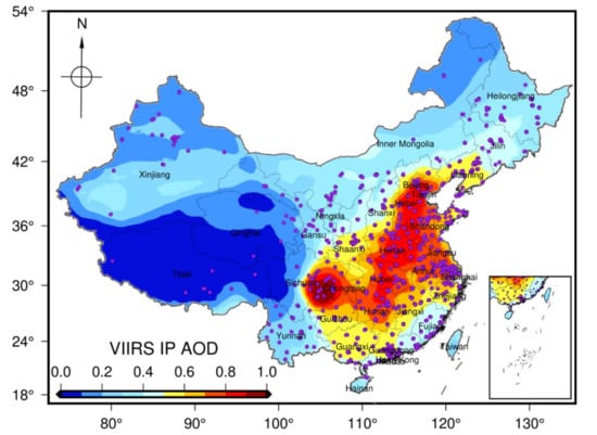
Figure 1.
Spatial distributions of the PM2.5 monitoring stations and annual mean VIIRS IP AOD data.
2.2. VIIRS IP AOD Data
The VIIRS instrument was designed to continue the heritage of MODIS and was equipped with a 13:30 ascending node to obtain global coverage on each day. The VIIRS IP AOD data at 550 nm were produced by using moderate bands and the AOD products during the period 2017–2018 were downloaded from the Comprehensive Large Array-data Stewardship System (CLASS). To reduce the impacts of data bias in VIIRS IP AOD for PM2.5 modeling, the AOD data with the best quality (flag = 0) were retained. The VIIRS IP AOD data retrieved on the same day were mosaicked and clipped to China extent with 750 m resolution using ArcGIS 10.3. Data Interpolating Empirical Orthogonal Functions (DINEOF) is a self-consistent and parameter-free interpolation method that can reconstruct missing data in both spatial fields and time series [46]. The DINEOF method has been widely used in various studies to fill data gaps [47,48]. Due to the low spatial coverage of daily VIIRS IP AOD data, we first used inverse distance weighted (IDW) to fill the small gaps in each day, and then applied the DINEOF method to reconstruct the full spatiotemporal coverage of VIIRS IP AOD data. Figure 1 depicts the annual mean values of VIIRS IP AOD, which indicates that the AOD values are higher in eastern China than in western China.
2.3. Meteorological Data
ERA5 is the fifth-generation atmospheric reanalysis model of global climate and provides hourly atmospheric estimates worldwide at a moderate resolution (0.1° or 0.25°). Meteorological data generated by ERA5 at the surface level during the period 2017–2018 were downloaded in this study, including 10 m wind components, 2 m air temperature (TEMP), total precipitation (TP), surface pressure (SP), boundary layer height (BLH), evaporation, and relative humidity (RH). We also computed the wind speed (WS) and wind direction (WD) based on the two wind components.
2.4. Geographical Data and Land Cover Data
Digital elevation model (DEM) with 90 m spatial resolution was obtained from the Shuttle Radar Topography Mission (SRTM). Normalized difference vegetation index (NDVI) indicating land cover, from 2017 to 2018 covering China with 500 m and 16 d resolutions retrieved from MODIS were achieved from the Level-1 and Atmospheric Archive and Distribution System (LAADS).
2.5. Population Data
Gridded population data of the world (GPWv4) with 5-year intervals during 1995–2020 are accessible at the National Aeronautics and Space Administration (NASA) Socioeconomic Data and Applications Center (SEDAC). The dataset of population count is produced as global grids at 30 arc-second resolution (~1 km). The annualized variation rate r is computed as:
where and are the population counts of the earlier and current censuses, and is the year span between two censuses. The population count in 2017 were then calculated by using the data in 2015 and 2020 as follows:
2.6. Data Preprocessing and Analysis
The experimental data included point datasets and raster datasets. The raster datasets were resampled to a 750 m grid (0.00625°) of China through bilinear interpolation. The PM2.5 measurements, VIIRS IP AOD data, and other auxiliary data were averaged to monthly scale for experiments. The pixel values of the raster datasets in the PM2.5 monitoring sites were then extracted to produce regression datasets of 12 months from 1 June 2017 to 31 May 2018. Correlation analysis and variance inflation factors (VIFs) were utilized to evaluate the statistical significance and collinearity among the parameters. Those variables with lower VIF values and higher Pearson’s r values were retained for spatial modeling. According to the results of explanatory analysis (Table S2), AOD, WS, TEMP, TP, BLH, RH, DEM, NDVI were used as explanatory variables since they were strongly correlated with PM2.5 and the VIF values suggested that their multicollinearity was rather weak.
3. Methods
The present work aims to map highly accurate and reasonable PM2.5 with 750 m resolution by using a newly developed GNNWR model. To evaluate its performance, the widely used GWR and GRNN were also performed for comparison and the OLR was used as a baseline model. Previous PM2.5 estimation researches evaluated model performance mainly using cross-validation (CV), which is not quite reliable to ensure its predictive ability [40]. Hence, a 10-fold CV and an external evaluation were adopted for the development of each model. In the modeling, the experimental data was spilt into a training dataset (85%) and a testing dataset (15%) for model calibration and evaluation. Each of the 10-fold CV models was implemented using 90% samples of the training dataset, with the rest 10% training samples for validation. The final model was built with the best parameters achieve by the 10-fold CV with all training samples. The testing dataset was used for the external evaluation of the final model. Model performance was evaluated using some metrics, including coefficient of determination (R2), root mean square error (RMSE), mean absolute error (MAE), mean absolute percentage error (MAPE) and mean error (Bias).
3.1. GNNWR Model
The structure of GNNWR for estimating the PM2.5–AOD relationship was built as follows:
were the coefficients of the OLR model, which reflected the average PM2.5–AOD relationship over China. The ordinary least squares (OLS) estimates of β were expressed as:
where
Then, the estimated value was calculated as:
where was a spatial weight matrix and was exactly calculated through the SWNN of GNNWR as follows [43]:
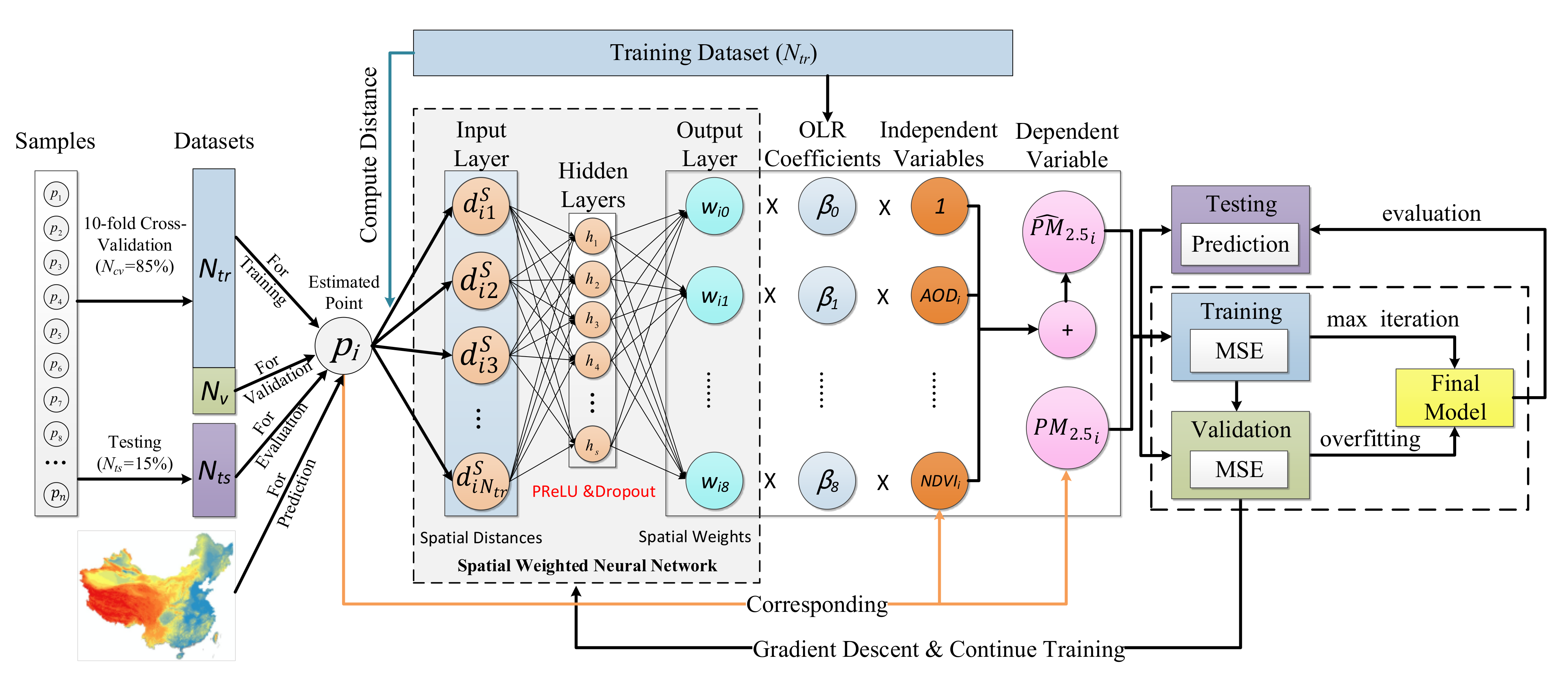
where denoted the spatial distance between point and all training points. Figure 2 illustrates the PM2.5 modeling process of GNNWR. The OLR coefficients representing the average PM2.5–AOD relationship in China were pre-calculated using the training dataset. The prediction accuracy of PM2.5 estimates was dependent on the non-linear fitting ability of SWNN, which was optimized through a grid search strategy (Supplementary Materials, SM). The neural network structure and hyper-parameters of GNNWR are shown in Table S3.

Figure 2.
The framework of the GNNWR model for PM2.5 estimations.
Moreover, we designed an adaptive learning rate strategy of stochastic gradient descent (SGD) for model training (Figure S1). First, a small learning rate was initialized and slowly increased to the maximum value with rate , which assured that the model gradually learns data features while avoided gradient explosion. Then, we accelerated the model training with the maximum learning rate. Finally, the learning rate exponentially declined by rate until the optimal model was achieved. In our experiments, , , , and were set to 0.1, 0.35, 0.05, and 0.98 as follows:
In addition, GNNWR used mean square error (MSE) as its loss function and was implemented based on Tensor Flow 1.6.0 and Python 3.7. The implementation details were described in SM and Figure S2.
3.2. GWR Model
The widely used GWR model was implemented to assess the performance of GNNWR with the following form:
where denoted the series coefficients of point . GWR captures the local effects through the spatially varying coefficients , which was calculated as follows:
where is an geographical weighting matrix with the diagonal elements representing non-stationary weights. A certain weight kernel of GWR should be specified to calculate the weight matrix. The widely used fixed Gaussian and adaptive bi-square weighting functions were adopted in our experiments. In addition, GWR used the corrected Akaike information criterion (AICc) value as its performance criterion to achieve the best model and was implemented in MATLAB 2013a.
3.3. GRNN Model
The GRNN contains four neural layers: input, hidden, summation and output layers. The input layer with neuron size equal to the length of independent variables is directly delivered to the hidden layer. The hidden layer has neurons equal to the count of training samples, and its transfer function is expressed as [49]:
where is the output of the hidden layer and is the parameter which should be optimized; is the input vector of point and is corresponding to the trainging sample. Then, two summations named and are calculated in the summation layer and the estimate in the output layer of GRNN is consequently represented as:
where and are the weighted and simple sums of the outputs from hidden layer, and is binding with the hidden neuron.
3.4. Population Weighted PM2.5
To explore the population exposures on fine-scale in China, the spatially population data were incorporated to calculate the population weighted PM2.5 (PPM2.5) at multiple administrative units (e.g., province, city and county):
where is the population-weighted PM2.5 at administrative unit i, and are the PM2.5 and population data of pixel j in administrative unit i.
4. Results
4.1. Descriptive Summary
Figure 3 displays the descriptive summaries and histograms of the monthly PM2.5 measurements and auxiliary datasets. The surface PM2.5 concentrations ranged from 2.45 to 339.00 μg/m3, with a mean value of 40.87 μg/m3 and a standard deviation (Std) of 22.56 μg/m3. The histogram of PM2.5 suggested that its value was mainly concentrated in the range of 0–50 μg/m3. The VIIRS IP AOD with a mean value of 0.61 was distributed in an extent of [0.01, 1.59]. It can be noted that the histograms of PM2.5 and AOD were somewhat dissimilar, mainly because their complex associations were significantly affected by geographical, meteorological, and seasonal conditions [6].
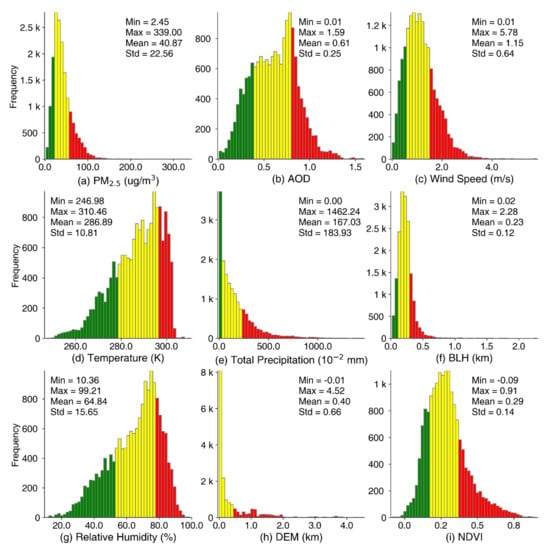
Figure 3.
Histograms and descriptive statistics of the experimental datasets. The green color represents the smaller 25% data, the yellow color represents the middle 50% data, and the red color represents the larger 25% data.
4.2. Model Performance
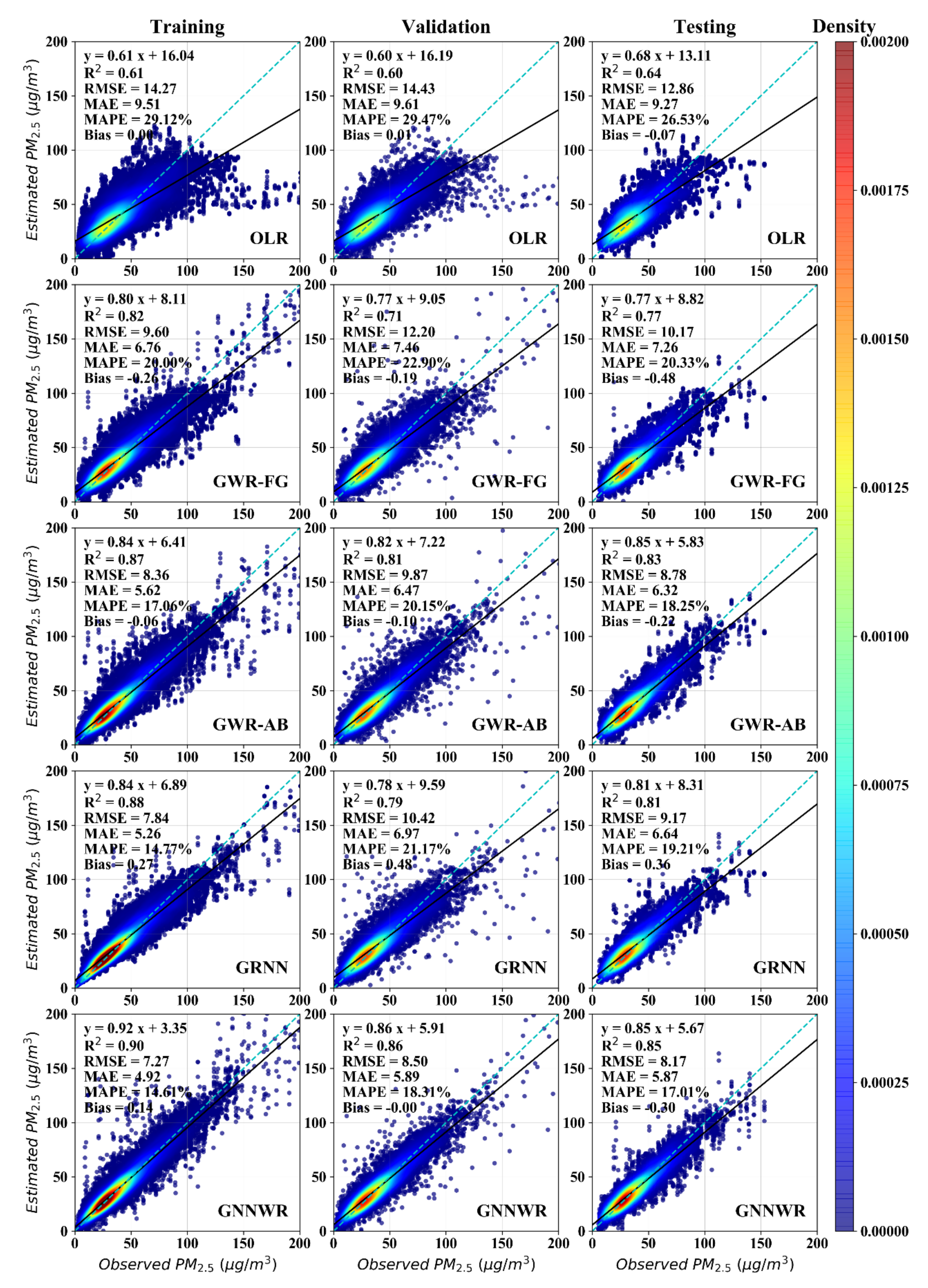
Table 1 displays the mean performance of PM2.5 estimations of monthly datasets for the OLR, GWR, GRNN and GNNWR models. Scatter plots of PM2.5 estimates versus observations among these methods are presented in Figure 4. We can see that GWR, GRNN and GNNWR models were far superior to the OLR model for all statistical indicators. Regarding the fitting performance of the 10-fold CV results, the training and validation accuracy of the GWR with adaptive bi-square kernel (GWR-AB) were better than the GWR with fixed Gaussian kernel (GWR-FG) according to the statistics of R2, RMSE, MAE and MAPE. This suggested that the adaptive kernel was more suitable than the fixed kernel to characterize the spatially non-stationary PM2.5–AOD relationship, which likely resulted from the uneven distribution of monitoring stations in China [50].

Table 1.
The 10-fold cross-validation and external evaluation performance of PM2.5 estimations for OLR, GWR, GRNN, and GNNWR.

Figure 4.
Scatter plots of the PM2.5 estimates versus the observations of different models: plots in the first, second and third columns are the fitting, validation and testing results, respectively.
Compared with the GWR-AB model, GRNN had higher training accuracy, but its validation performance was inferior. For example, GRNN increased the training R2 of GWR-AB from 0.87 to 0.88 and decreased the training RMSE and MAE values from 8.36 and 5.62 µg/m3 to 7.84 and 5.26 µg/m3. However, the CV R2 of GWR-AB (0.81) was higher than GRNN (0.79) and its CV RMSE and MAE (9.87 and 6.47 µg/m3) were lower than GRNN (10.42 and 6.97 µg/m3). It was worth noting that the training and validation accuracies of GNNWR were higher than GWR and GRNN. Comparing with the best comparison indicators, GNNWR improved the training R2 and RMSE of GRNN from 0.88 and 7.83 µg/m3 to 0.90 and 7.27 µg/m3, while the CV R2 and RMSE of GWR-AB were considerably enhanced from 0.81 and 9.87 µg/m3 to 0.86 and 8.50 µg/m3 of GNNWR.
The prediction performance assessed by the external evaluation of testing dataset illustrated good agreement with the results assessed by the 10-fold CV (Table 1). Although the predictive indicators of OLR was still the worst among the models, its prediction performance was better than its fitting performance. This suggests that OLR does not suffer from overfitting. Comparing the prediction accuracy between GWR and GRNN, GWR-AB achieved the highest prediction performance and GRNN ranked second better than GWR-FG. Table 1 also revealed that the prediction indicators of GNNWR were superior to GWR and GRNN. Compared with the best comparison model (i.e., GWR-AB), the predictive R2 was raised from 0.83 to 0.85 and the predictive RMSE, MAE and MAPE were declined at least 7%. Similar differences in model performance among the methods were noted in Figure 4. The scatter plots of OLR were most dispersive consistent with its worst performance. GWR and GRNN exhibited high estimation accuracy for low values but commonly underestimated high values. For the GNNWR model, its estimates showed the best fitting and prediction precision and less encountered unreasonable underestimation and overestimation.
In the meantime, it was unexpected that the mean estimated bias of OLR was very small and close to 0 (Table 1), which was much better than the other models. However, the scatter plots of OLR (Figure 4) indicated that its underestimation of high values was quite severe. To investigate the potential reason, we further evaluated model performance in the subsets of estimates, including PM2.5 concentration within 0–50 μg/m3, 50–100 μg/m3 and >100 μg/m3 as shown in Table 2. We can clearly observe that all models had a tendency of overestimating at low values while underestimating at high values. The mean bias of OLR showed that its biases at both low and high values were greater than other models, which verified its worst performance. We therefore speculated that the positive bias of OLR at low values and its negative bias at high values happened to cause its overall bias to be small. The estimation performance of GNNWR was the best for all subsets according to RMSE, MAE and MAPE values. Further, the estimated bias of GNNWR was also smaller than other models, especially for high values. Figures S3–S5 show the statistical indicators of model performance for OLR, GWR, GRNN and GNNWR in each month. It can be obviously noticed that the R2 values of GNNWR were the highest while its RMSE, MAE and MAPE values were lowest among the models for almost all months, demonstrating its excellent ability and robustness to capture spatial non-stationarity and complex non-linearity in the PM2.5–AOD relationship.

Table 2.
Model performance with PM2.5 concentrations in certain extents.
4.3. Annual Mapping and Seasonal Variations
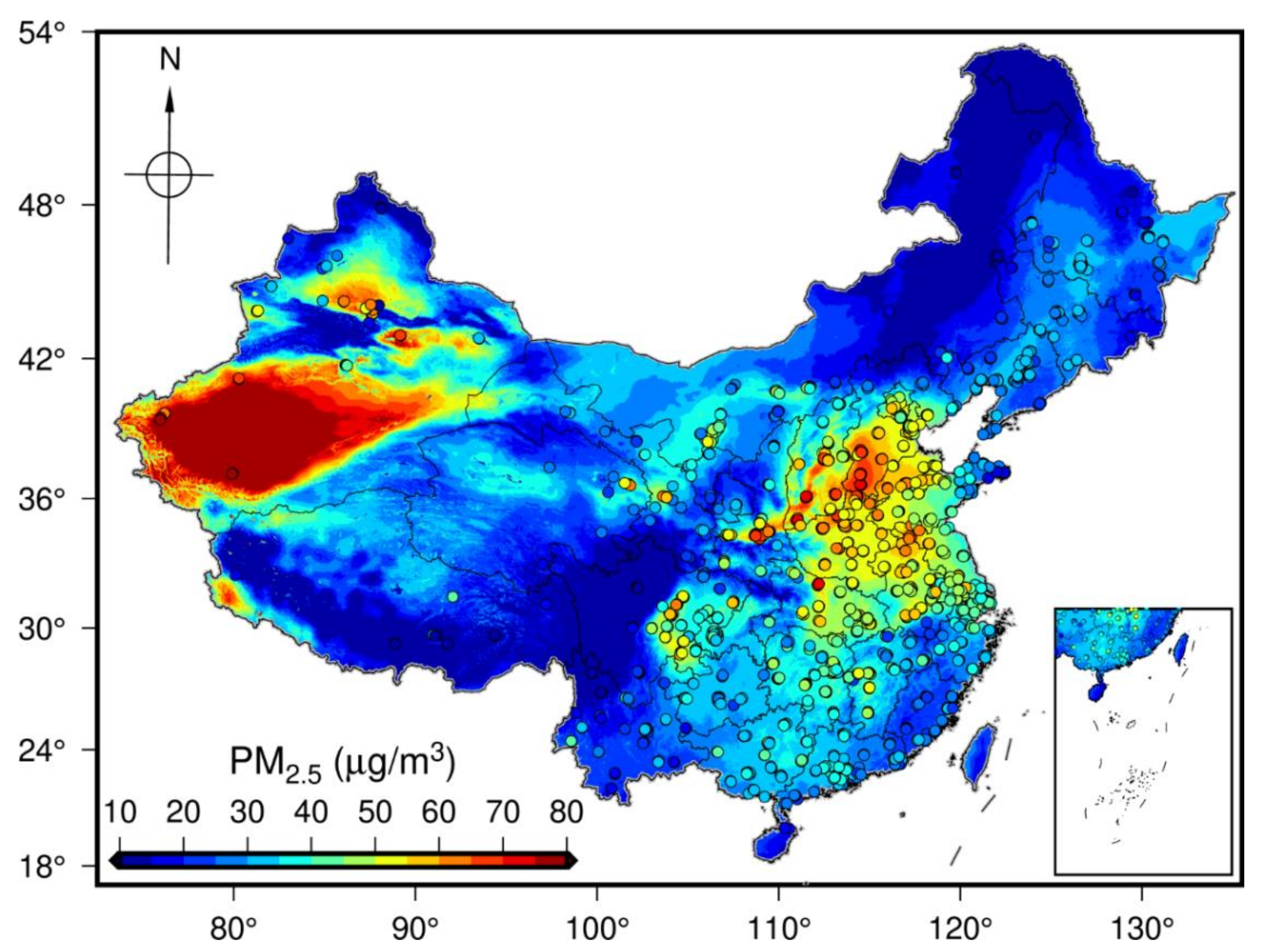
Figure 5 displays the spatial mappings of annual mean satellite-estimated PM2.5 obtained by GNNWR, and ground-measured PM2.5 in China. The spatial varying pattern of the satellite-derived PM2.5 estimates agreed well with ground-level observations, which was also consistent with the previous studies [16,17,51]. Notably, GNNWR has obtained almost complete spatial coverage of PM2.5 estimates thanks to the spatiotemporal interpolation of the missing data of VIIRS IP AOD. More specifically, the annual mean PM2.5 concentration was 31.07 ± 17.52 µg/m3 and heavy pollutions were mainly located in Hebei, Henan, and Shandong Provinces, which were thought to result from the rapidly economic development and highly accelerated urbanization [6]. The Taihang Mountains in Hebei Province also hampered the PM2.5 dispersions, further aggravating air pollutions in these areas [16]. High PM2.5 concentrations as well appeared in the Xinjiang Autonomous Region due to the great quantity of dust aerosols coming from the Taklimakan Desert [17,52,53]. By contrast, the southern and northern provinces exhibited much better air quality with PM2.5 concentrations basically below 30 µg/m3, such as Hainan, Guangdong, and Heilongjiang Provinces. In all, ~30% areas of China exceeded the Chinese air quality standard of Level II (35 µg/m3).

Figure 5.
Spatial mappings of annual mean ground-measured and satellite-estimated PM2.5 concentrations in China.
Figure 6 shows the maps of seasonal mean PM2.5 concentrations achieved by GNNWR, which also covered almost the entire range of China. Significant seasonal variations were observed with the heaviest pollution in winter and relatively low pollution in summer. The average PM2.5 in winter was 42.30 ± 25.21 µg/m3 with >55% areas exceeding the Chinese air quality standard of Level II. This was mainly caused by the coal burning of heating systems in northern China and the unfavorable weather for pollutant dispersion in eastern China [54,55,56]. In summer, China showed the best air quality (20.12 ± 11.54 µg/m3) with only 8.92% areas higher than the Chinese air quality standard of Level II. The primary explanation was that the abundant clean air and sufficient precipitation in summer greatly improved the air quality [16]. In addition, the high vegetation covers in summer helped the absorption of air pollutants, which also reduced the PM2.5 concentrations to a certain extent [6]. The PM2.5 in spring was higher than the annual mean with an average value of 35.77 ± 28.74 µg/m3 and the mean PM2.5 in autumn was 26.82 ± 16.78 µg/m3. Nevertheless, the PM2.5 pollutions in China have been considerable reduced compared to previous studies performed in early years [6,7,17,26].
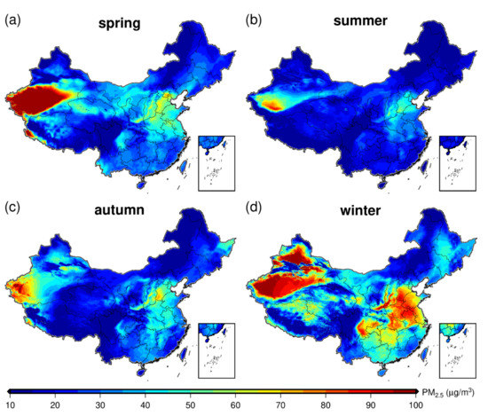
Figure 6.
Seasonal variation of satellite-estimated PM2.5 concentrations in China. (a) spring (b) summer (c) autumn (d) winter.
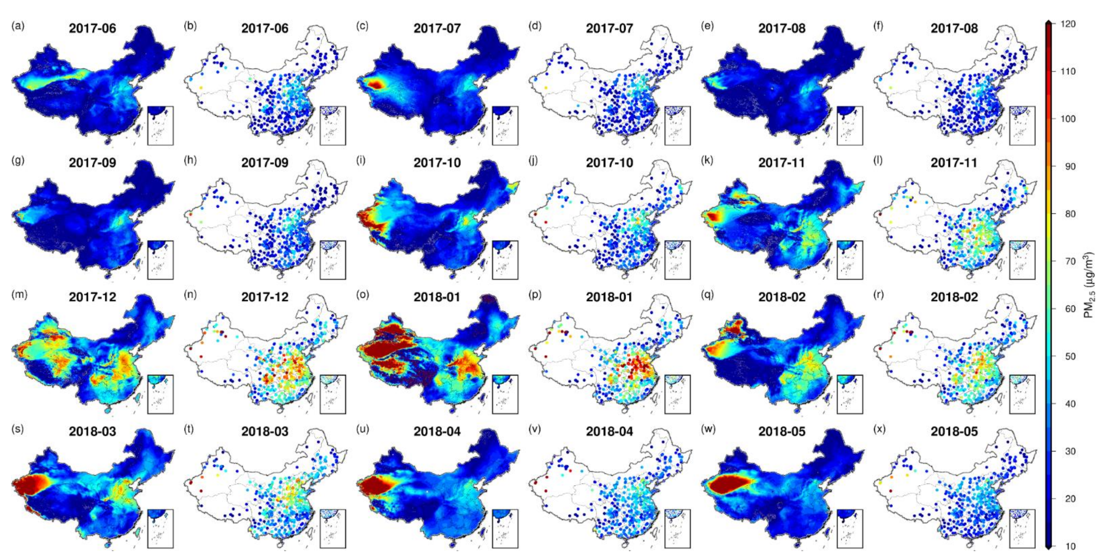
Since the GNNWR model was built on a monthly scale, the spatial mappings of monthly satellite-estimated and ground-measured PM2.5 in China are presented in Figure 7. The satellite-estimated PM2.5 agreed spatially well with the ground-measured observations in each month. Spatial discrepancies in PM2.5 pollutions were noticeable on monthly scale. The most severe PM2.5 pollution is in January of winter (52.38 ± 46.16 µg/m3) with ~60% of the country exceeding the Chinese air quality standard of Level II. By contrast, the August of summer experiences the lightest air pollution (15.68 ± 11.56 µg/m3) with only ~5% areas exceeding the air quality standard.

Figure 7.
Spatial mappings of monthly satellite-estimated and ground-measured PM2.5 concentrations in China.
5. Discussion
5.1. Applicability and Superiority of the GNNWR Model
Satellite-retrieved aerosol optical depth (AOD) data are extensively integrated with ground-level measurements to achieve spatially continuous fine PM2.5 distributions [7,8,9,10,11,12,13,14,15,16]. Current satellite-based methods however face challenges in obtaining highly accurate and reasonable PM2.5 distributions due to the inability to handle both spatial non-stationarity and complex non-linearity in the PM2.5–AOD relationship. This study therefore developed a satellite-based spatially neural network weighted regression model (i.e., GNNWR) to achieve highly accurate and reasonable satellite-derived PM2.5 mapping with fine resolution (<1 km) across the entire China.
Table 1 has shown that the performance of the GWR, GRNN and GNNWR models were far superior to the OLR model, which manifests significant non-stationarity and non-linearity indeed in the PM2.5 modelling. The GRNN model presented higher training accuracy than the GWR-AB model, but its validation performance was inferior, suggesting that although GRNN could enhance the training accuracy of PM2.5–AOD relationship through its non-linear fitting capability, it may encounter severe overfitting problem since it does not take spatial effects into account. At the meantime, the higher training and validation accuracies of GNNWR than GWR and GRNN, demonstrates that GNNWR is more powerful than GWR and GRNN in fitting PM2.5–AOD relationship. It also suggests that the SWNN in GNNWR is superior to the spatial kernel of GWR in constructing spatially non-stationary weights [43]. Furthermore, the validation and prediction accuracies of GNNWR were even comparable to the training accuracy of GWR-AB and much closer to its training performance than GRNN. This demonstrates that the newly developed GNNWR robustly captured spatial non-stationarity and complex non-linearity in the PM2.5–AOD relationship and obtained an excellent prediction capacity for PM2.5 modelling. The higher estimation accuracies and smaller estimated biases of GNNWR than other models for all subsets in Table 2 further indicates its broad applicability in PM2.5 modelling.
Compared to previous works that integrated MODIS and MAIAC AOD products to map high-resolution PM2.5 across the entire China, the prediction performance of our GNNWR model (CV and predictive R2 of 0.86 and 0.85) was superior to most earlier studies with CV R2 of 0.64-0.83 [6,12,16,27,57,58] and was also comparable to recent studies with CV R2 of 0.76-0.89 [17,36,42,59,60]. Since the data accuracy of VIIRS IP AOD was somehow inferior to the MODIS and MAIAC AOD products, these results also demonstrated the robust predictive power of GNNWR for modeling the PM2.5–AOD relationship.
5.2. Accuracy and Reasonability of Satellite-Derived PM2.5 Mappings
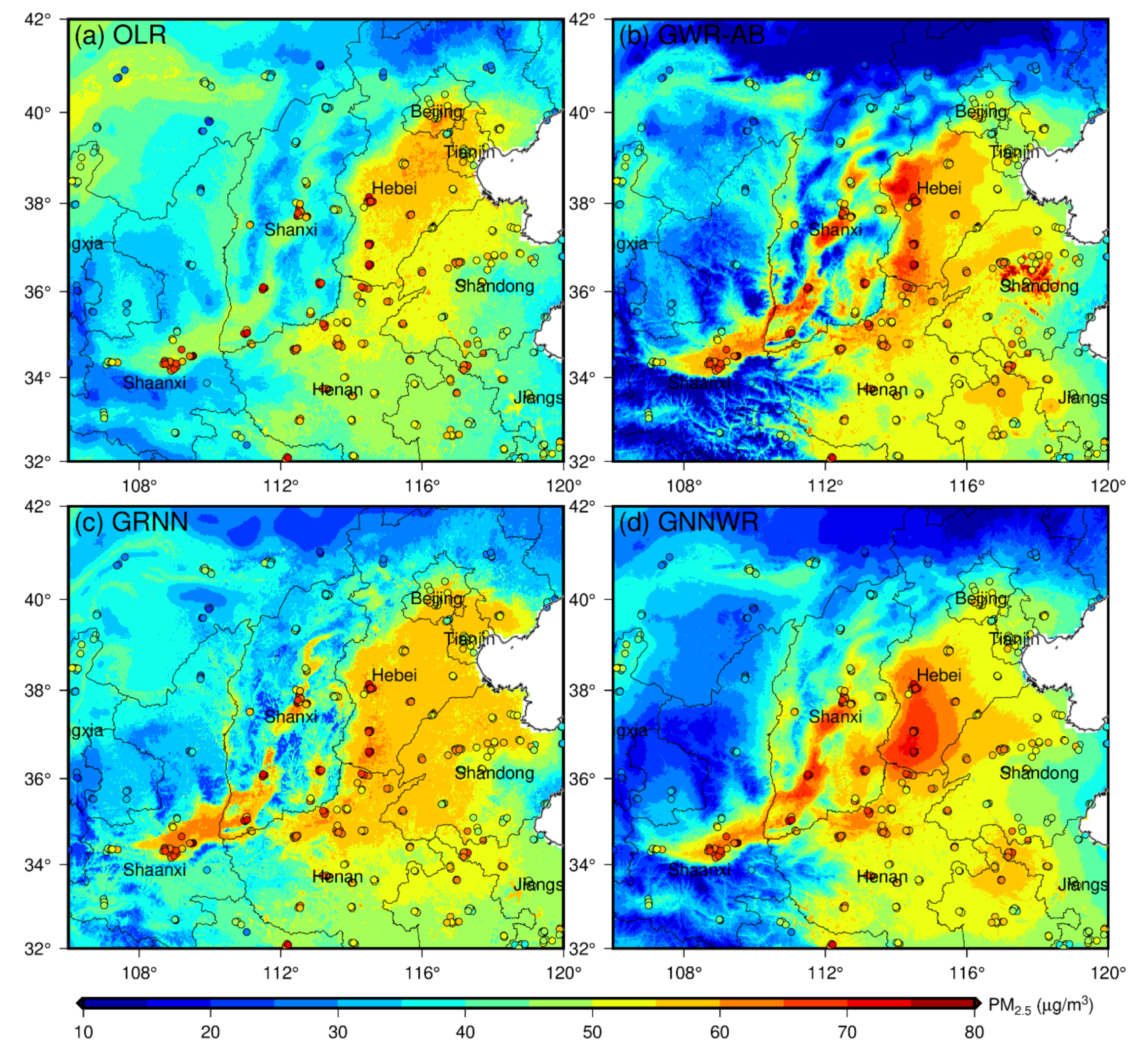
To assess the accuracy and reasonability of satellite-derived PM2.5 mappings of GNNWR, annual mean PM2.5 maps of China achieved by OLR, GWR, and GRNN are depicted for comparison (Figure S6). It can be noted that the spatial PM2.5 maps of these models were basically consistent. The OLR estimates exhibited homogenous trends in space due to its inconsideration of spatial non-stationarity while the GRNN estimates displayed some unreasonable variations in western China caused by its overfitting. Obviously, the maps of GWR-AB and GNNWR were more reasonable and coincident with the ground-level measurements. The North China Plain is a highly developed and polluted area in China and is of great concern to the public [15,61]. The satellite-derived PM2.5 estimates of these models in this area are amplified for detailed comparison (Figure 8). We can see that OLR and GRNN were unable to portray the high PM2.5 concentrations (>60 µg/m3) in heavily polluted areas due to their serious underestimation of high values. Although GWR-AB was capable of mapping high PM2.5 and displayed a better distribution than OLR and GRNN, its spatial varying pattern was too steep and showed some unreasonable distributions, such as the high-value aggregation in Shandong Province and the drastic mutation in Shanxi Province. It was clear that GNNWR has obtained highly accurate estimates and rarely exhibited unreasonable variations benefited from its excellent prediction ability.
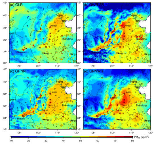
Figure 8.
Regional comparison of annual mean satellite-estimated PM2.5 of different models in the North China Plain.
5.3. Analysis of Fine-Scale Population Exposures at Multiple Levels
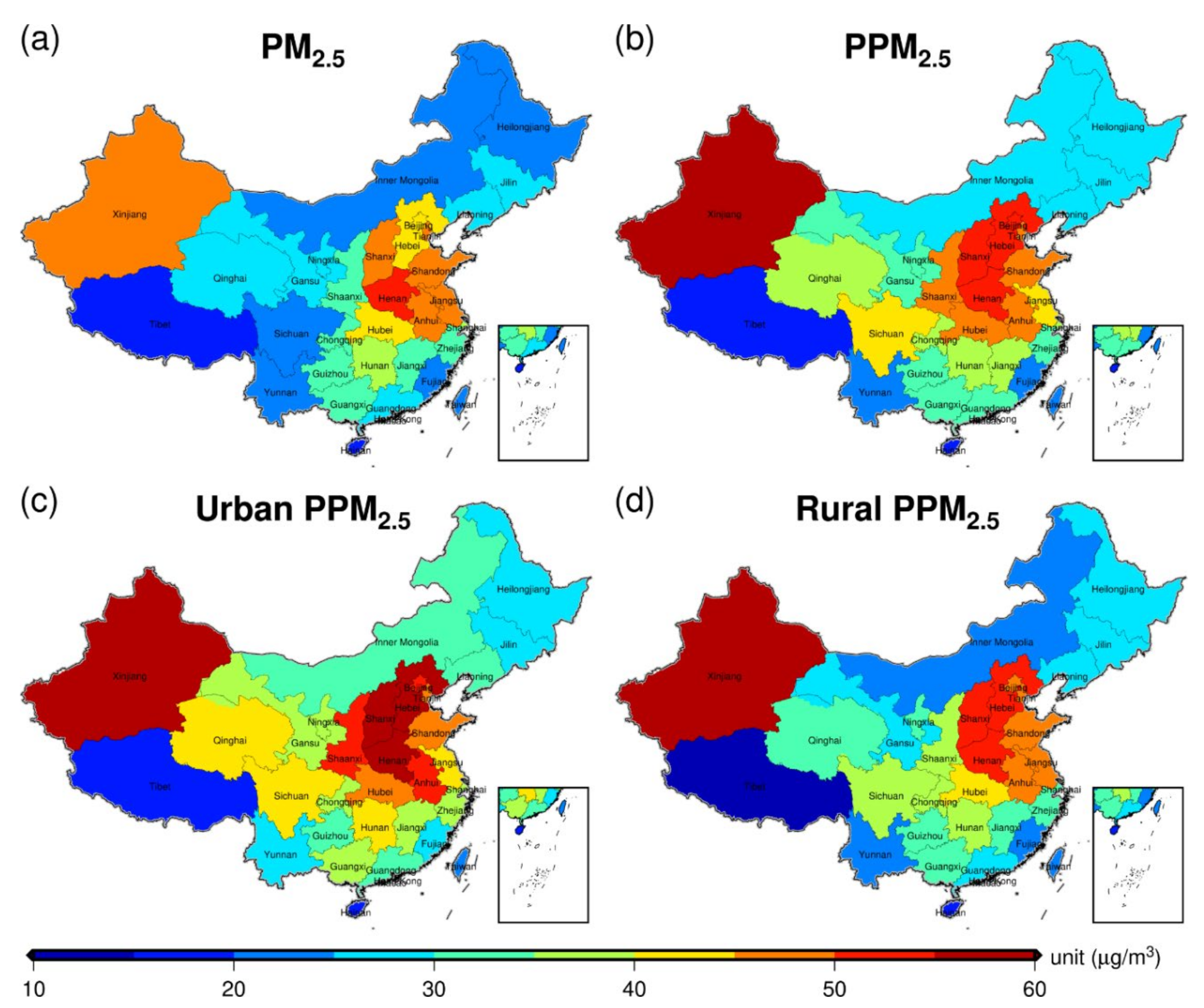
High spatial resolution PM2.5 datasets advance the full estimation of population exposure (i.e., PPM2.5) with smaller bias produced by the averaging within each pixel [62,63]. By resampling our 750 m resolution PM2.5 product to a 1 km grid and linking it with the GPWv4 population estimates, the annual mean PPM2.5 concentrations at province level were calculated (Figure 9 and Table S4). Based on the urbanization calculation method proposed by [62], the urban areas in China were measured by the population density exceeding 600 people/km² (Figure S7). Consequently, the PM2.5 exposures for both urban and rural areas were also estimated to comprehensively explore the air pollution levels in China.

Figure 9.
Spatial mappings of (a) annual mean PM2.5, (b) population weighted PM2.5 (PPM2.5), (c) urban PPM2.5 and (d) rural PPM2.5 concentrations at province level in China.
We can note that the annual mean PPM2.5 was higher than the PM2.5 in most provinces and the PPM2.5 in Xinjiang, Hebei, Shanxi, Henan and Beijing were more than 50 µg/m3. Surprisingly, although the mean population of Xinjiang Autonomous Region was quite small, its annual mean PPM2.5 was the highest of 63.27 µg/m3, suggesting that most people in the Xinjiang Autonomous Region were located in the high PM2.5 areas. In addition, Sichuan Province has greatly increased its PM2.5 from 20.09 µg/m3 to 40.08 µg/m3 of PPM2.5 with a growth rate of ~100%, which also demonstrated that the population in Sichuan Province was mainly concentrated in highly polluted areas. Although the urban areas were much smaller than rural areas in China (Figure S7), the urban PPM2.5 was significantly higher than the rural PPM2.5 for almost all provinces, except Xinjiang, Tianjin, and Jiangsu. The urban PPM2.5 in most provinces exceeded the Chinese air quality standard of Level II and the high PM2.5 exposures were primarily concentrated in the North China Plain (>55 µg/m3). This manifested that urban residents were facing severer PM2.5 pollutions and higher health risks than rural residents in China. More efforts are urgently needed to further control the PM2.5 emissions in Chinese urban areas.
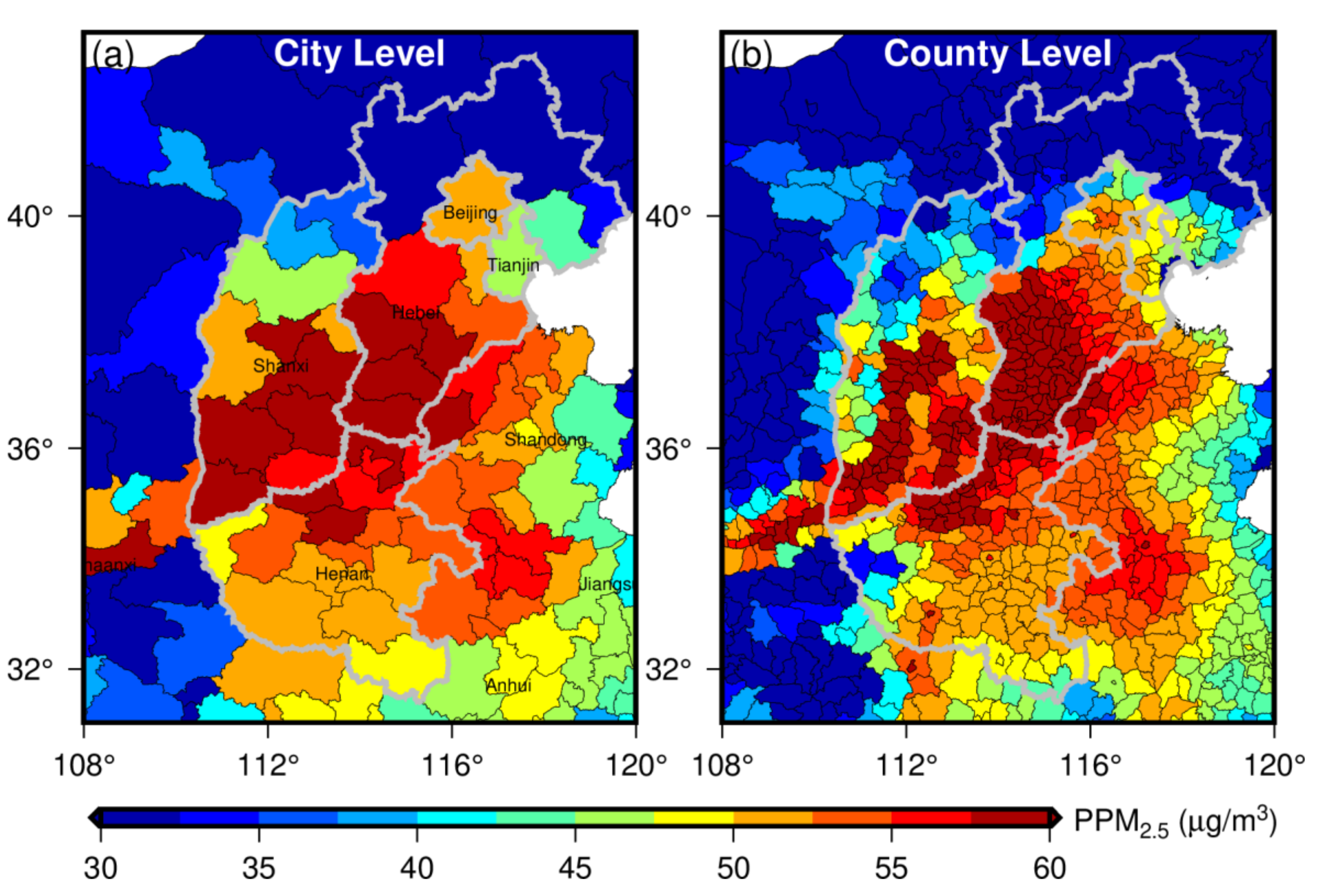
The high-resolution PM2.5 product enabled us to investigate air pollutions in urban cities on more fine-scale. The annual mean PPM2.5 concentrations at the city and county levels in the North China Plain were calculated to study the detailed exposures in highly polluted areas of China (Figure 10). From the view of the city level, the high PPM2.5 areas (>57.5 µg/m3) were aggregated and mainly located in southern Hebei, southern Shanxi and northern Henan. Beijing and Tianjin showed lower PPM2.5 than the southern Hebei, mainly attributed to the strict control policies of local governments in recent years. The PPM2.5 at the county level presented more detailed spatial patterns. Figure 10b illustrated that the high PPM2.5 areas in southern Hebei Province were more agglomerate than Shanxi and Henan Provinces, indicating the heaviest PM2.5 pollutions and highest health risks in these areas.
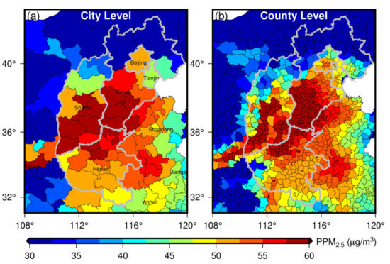
Figure 10.
Spatial distributions of population weighted PM2.5 (PPM2.5) concentrations at the city and county levels in the North China Plain.
6. Conclusions
To obtain highly accurate and reasonable satellite-derived PM2.5 mapping with fine resolution (<1 km) across the entire China, this study developed a satellite-based spatially neural network weighted regression model (i.e., GNNWR) to deal with both spatial non-stationarity and complex non-linearity in PM2.5–AOD modelling. Our work was the first to use the high-resolution VIIRS IP AOD to predict 750 m resolution PM2.5 concentrations over large-scale in China. The newly developed GNNWR model presented obvious advantages in PM2.5 estimations because it overcame the defect of GWR to address complex non-linear features and enabled the neural network to handle spatial effects in the PM2.5–AOD relationship.
The model performance of GNNWR was fully assessed through a 10-fold CV and an external evaluation by comparing it with the OLR, GWR and GRNN methods. The GNNWR model achieved the highest performance for both fitting (training R2 = 0.90, RMSE = 7.27 µg/m3 and CV R2 = 0.86, RMSE = 8.50 µg/m3) and prediction (R2 = 0.85, RMSE = 8.16 µg/m3). Detailed comparison of spatial mappings also indicated that GNNWR obtained superior prediction accuracy and rarely exhibited unreasonable variations. Although the data accuracy of VIIRS IP AOD was somehow inferior to the MODIS and MAIAC AOD, the prediction performance of GNNWR was comparable to most previous studies conducted across the entire China, further demonstrating its robust predictive power of PM2.5 modeling. The potential of VIIRS IP AOD to estimate PM2.5 with complex dispersions over large-scale has also been validated.
Our newly generated PM2.5 data in China had higher spatial resolution (750 m) than most existing products and provided almost complete spatial coverage, which are valuable to advance environmental and health research in China. The spatial mapping of our PM2.5 product showed that the PM2.5 pollutions in China has been greatly improved in 2018 with annual mean concentration of 31.07 ± 17.52 µg/m3. Nonetheless, the fine-scale PM2.5 exposures suggested that the PM2.5 pollutions in most urban areas were still severe, especially in southern Hebei Province. More efforts are therefore needed for controlling PM2.5 emissions in these populated and developed areas in the future.
Supplementary Materials
The following are available online at https://www.mdpi.com/article/10.3390/rs13101979/s1, Section S1: Neural network architecture optimization of GNNWR model, Section S2: Training and validation procedures of the GNNWR model, Figure S1: Adaptive learning rate strategy for the GNNWR model, Figure S2: Training and validation procedures of the GNNWR model for PM2.5–AOD modeling, Figure S3: Training performance of PM2.5 estimations in each month of the GNNWR model, Figure S4: Cross-validation performance of PM2.5 estimations in each month of the GNNWR model, Figure S5: Prediction performance of PM2.5 estimations in each month of the GNNWR model, Figure S6: Spatial distributions of annual mean ground-measured (a) PM2.5 concentrations and satellite-estimated (b–f) PM2.5 concentrations of different models in China, Figure S7: Spatial distributions of population count in 2017 and the urban and rural areas estimated from the population counts in China, Table S1: Data sources and descriptions of the datasets, Table S2: Exploratory analysis of PM2.5 and the explanatory variables, Table S3: Settings for the architectures and hyper-parameters for the GNNWR model, Table S4. Annual mean and population weighted PM2.5 (PPM2.5) concentrations at province level in China. The PPM2.5 includes the whole, urban and rural PPM2.5. Rate is the variation rate from the mean PM2.5 to the whole PPM2.5. U/R is the ratio of urban PPM2.5 and rural PPM2.5.
Author Contributions
Conceptualization, Y.C. and S.W.; methodology, Y.C.; validation, Y.C. and Y.W.; investigation, Y.C. and Y.W.; resources, S.W. and Z.D.; writing—original draft preparation, Y.C.; supervision, S.W. and Y.W.; project administration, S.W., F.Z., and Z.D.; funding acquisition, S.W., F.Z., R.L. and Z.D. All authors have read and agreed to the published version of the manuscript.
Funding
This research was supported by by the National Natural Science Foundation of China [No. 41922043, No. 41871287, No. 42001323], National Key Research and Development Program of China [No. 2018YFB0505000].
Data Availability Statement
The data presented in this study can be available at: https://figshare.com/s/2a52b41ebf9442fd5d1f accessed on 4 May 2021.
Conflicts of Interest
The authors declare no conflict of interest.
References
- Dominici, F.; Peng, R.D.; Bell, M.L.; Pham, L.; McDermott, A.; Zeger, S.L.; Samet, J.M. Fine particulate air pollution and hospital admission for cardiovascular and respiratory diseases. JAMA 2006, 295, 1127–1134. [Google Scholar] [CrossRef]
- Bartell, S.M.; Longhurst, J.; Tjoa, T.; Sioutas, C.; Delfino, R.J. Particulate air pollution, ambulatory heart rate variability, and cardiac arrhythmia in retirement community residents with coronary artery disease. Environ. Health Persp. 2013, 121, 1135–1141. [Google Scholar] [CrossRef]
- Peng, J.; Chen, S.; Lü, H.; Liu, Y.; Wu, J. Spatiotemporal patterns of remotely sensed PM2.5 concentration in China from 1999 to 2011. Remote Sens. Environ. 2016, 174, 109–121. [Google Scholar] [CrossRef]
- Chang, Y. China needs a tighter PM2.5 limit and a change in priorities. Environ. Sci. Technol. 2012, 46, 7069–7070. [Google Scholar] [CrossRef]
- Liu, M.; Zhou, G.; Saari, R.K.; Li, S.; Liu, X.; Li, J. Quantifying PM2.5 mass concentration and particle radius using satellite data and an optical-mass conversion algorithm. ISPRS J. Photogramm. Remote Sens. 2019, 158, 90–98. [Google Scholar] [CrossRef]
- Ma, Z.; Hu, X.; Huang, L.; Bi, J.; Liu, Y. Estimating ground-level PM2.5 in China using satellite remote sensing. Environ. Sci. Technol. 2014, 48, 7436–7444. [Google Scholar] [CrossRef] [PubMed]
- You, W.; Zang, Z.; Zhang, L.; Li, Y.; Wang, W. Estimating national-scale ground-level PM2.5 concentration in China using geographically weighted regression based on MODIS and MISR AOD. Environ. Sci. Pollut. Res. 2016, 23, 8327–8338. [Google Scholar] [CrossRef]
- Hu, Z. Spatial analysis of MODIS aerosol optical depth, PM2.5, and chronic coronary heart disease. Int. J. Health Geogr. 2009, 8, 27. [Google Scholar] [CrossRef] [PubMed]
- Song, W.; Jia, H.; Huang, J.; Zhang, Y. A satellite-based geographically weighted regression model for regional PM2.5 estimation over the Pearl River Delta region in China. Remote Sens. Environ. 2014, 154, 1–7. [Google Scholar] [CrossRef]
- Lv, B.; Hu, Y.; Chang, H.H.; Russell, A.G.; Bai, Y. Improving the Accuracy of Daily PM2.5 Distributions Derived from the Fusion of Ground-Level Measurements with Aerosol Optical Depth Observations, a Case Study in North China. Environ. Sci. Technol. 2016, 50, 4752–4759. [Google Scholar] [CrossRef] [PubMed]
- Guo, Y.; Tang, Q.; Gong, D.; Zhang, Z. Estimating ground-level PM2.5 concentrations in Beijing using a satellite-based geographically and temporally weighted regression model. Remote Sens. Environ. 2017, 198, 140–149. [Google Scholar] [CrossRef]
- Yu, W.; Liu, Y.; Ma, Z.; Bi, J. Improving satellite-based PM2.5 estimates in China using Gaussian processes modeling in a Bayesian hierarchical setting. Sci. Rep. 2017, 7, 7048. [Google Scholar] [CrossRef] [PubMed]
- Li, L.; Zhang, J.; Meng, X.; Fang, Y.; Ge, Y.; Wang, J.; Wang, C.; Wu, J.; Kan, H. Estimation of PM2.5 concentrations at a high spatiotemporal resolution using constrained mixed-effect bagging models with MAIAC aerosol optical depth. Remote Sens. Environ. 2018, 217, 573–586. [Google Scholar] [CrossRef]
- Chen, W.; Ran, H.; Cao, X.; Wang, J.; Teng, D.; Chen, J.; Zheng, X. Estimating PM2. 5 with high-resolution 1-km AOD data and an improved machine learning model over Shenzhen, China. Sci. Total Environ. 2020, 746, 141093. [Google Scholar] [CrossRef]
- Yao, F.; Si, M.; Li, W.; Wu, J. A multidimensional comparison between MODIS and VIIRS AOD in estimating ground-level PM2.5 concentrations over a heavily polluted region in China. Sci. Total Environ. 2018, 618, 819–828. [Google Scholar] [CrossRef] [PubMed]
- He, Q.; Huang, B. Satellite-based mapping of daily high-resolution ground PM2.5 in China via space-time regression modeling. Remote Sens. Environ. 2018, 206, 72–83. [Google Scholar] [CrossRef]
- Wei, J.; Huang, W.; Li, Z.; Xue, W.; Peng, Y.; Sun, L.; Cribb, M. Estimating 1-km-resolution PM2.5 concentrations across China using the space-time random forest approach. Remote Sens. Environ. 2019, 231, 111221. [Google Scholar] [CrossRef]
- Li, L. A robust deep learning approach for spatiotemporal estimation of satellite AOD and PM2.5. Remote Sens. 2020, 12, 264. [Google Scholar] [CrossRef]
- Cao, C.; De Luccia, F.J.; Xiong, X.; Wolfe, R.; Weng, F. Early on-orbit performance of the visible infrared imaging radiometer suite onboard the Suomi National Polar-Orbiting Partnership (S-NPP) satellite. Geosci. Remote 2013, 52, 1142–1156. [Google Scholar] [CrossRef]
- Yao, F.; Wu, J.; Li, W.; Peng, J. Estimating Daily PM2. 5 Concentrations in Beijing Using 750-M VIIRS IP AOD Retrievals and a Nested Spatiotemporal Statistical Model. Remote Sens. 2019, 11, 841. [Google Scholar] [CrossRef]
- Cao, C.; Xiong, J.; Blonski, S.; Liu, Q.; Uprety, S.; Shao, X.; Bai, Y.; Weng, F. Suomi NPP VIIRS sensor data record verification, validation, and long-term performance monitoring. J. Geophys. Res. Atmos. 2013, 118, 664–678. [Google Scholar] [CrossRef]
- Ma, Y.; Liu, B.; Gong, W.; Shi, Y.; Jin, S. Impact of environmental pollution on the retrieval of AOD products from Visible Infrared Imaging Radiometer Suite (VIIRS) over wuhan. Atmos. Pollut. Res. 2019, 10, 2063–2071. [Google Scholar] [CrossRef]
- Xiao, Q.; Zhang, H.; Choi, M.; Li, S.; Kondragunta, S.; Kim, J.; Holben, B.; Levy, R.C.; Liu, Y. Evaluation of VIIRS, GOCI, and MODIS Collection 6 AOD retrievals against ground sunphotometer observations over East Asia. Atmos. Chem. Phys. 2016, 16, 1255. [Google Scholar] [CrossRef]
- Gupta, P.; Christopher, S.A. Particulate matter air quality assessment using integrated surface, satellite, and meteorological products: Multiple regression approach. J. Geophys. Res. Atmos. 2009, 114, D14. [Google Scholar] [CrossRef]
- Benas, N.; Beloconi, A.; Chrysoulakis, N. Estimation of urban PM10 concentration, based on MODIS and MERIS/AATSR synergistic observations. Atmos. Environ. 2013, 79, 448–454. [Google Scholar] [CrossRef]
- Xiao, L.; Lang, Y.; Christakos, G. High-resolution spatiotemporal mapping of PM2.5 concentrations at Mainland China using a combined BME-GWR technique. Atmos. Environ. 2018, 173, 295–305. [Google Scholar] [CrossRef]
- You, W.; Zang, Z.; Zhang, L.; Li, Y.; Pan, X.; Wang, W. National-scale estimates of ground-level PM2.5 concentration in China using geographically weighted regression based on 3 km resolution MODIS AOD. Remote Sens. 2016, 8, 184. [Google Scholar] [CrossRef]
- Hu, X.; Waller, L.A.; Al-Hamdan, M.Z.; Crosson, W.L.; Estes, M.G.; Estes, S.M.; Quattrochi, D.A.; Sarnat, J.A.; Liu, Y. Estimating ground-level PM2.5 concentrations in the southeastern US using geographically weighted regression. Environ. Res. 2013, 121, 1–10. [Google Scholar] [CrossRef] [PubMed]
- Zhai, L.; Li, S.; Zou, B.; Sang, H.; Fang, X.; Xu, S. An improved geographically weighted regression model for PM2.5 concentration estimation in large areas. Atmos. Environ. 2018, 181, 145–154. [Google Scholar] [CrossRef]
- Memarianfard, M.; Hatami, A.M.; Memarianfard, M. Artificial neural network forecast application for fine particulate matter concentration using meteorological data. Glob. J. Environ. Sci. Manag. 2017, 3, 333–340. [Google Scholar]
- Shen, H.; Li, T.; Yuan, Q.; Zhang, L. Estimating regional ground-Level PM2.5 directly from satellite top-of-atmosphere reflectance using deep belief networks. J. Geophys. Res. Atmos. 2018, 123, 13875–13886. [Google Scholar] [CrossRef]
- Ceylan, Z.; Bulkan, S. Forecasting PM10 levels using ANN and MLR: A case study for Sakarya City. Glob. NEST J. 2018, 20, 281–290. [Google Scholar]
- Chen, Y. Prediction algorithm of PM2.5 mass concentration based on adaptive BP neural network. Computing 2018, 100, 825–838. [Google Scholar] [CrossRef]
- Lyu, H.; Dai, T.; Zheng, Y.; Shi, G.; Nakajima, T. Estimation of PM2.5 concentrations over Beijing with MODIS AODs using an artificial neural network. Sola 2018, 14, 14–18. [Google Scholar] [CrossRef]
- Li, J.; Jin, M.; Li, H. Exploring spatial influence of remotely sensed PM2.5 concentration using a developed deep convolutional neural network model. Int. J. Environ. Res. Public Health 2019, 16, 454. [Google Scholar] [CrossRef]
- Wang, W.; Zhao, S.; Jiao, L.; Taylor, M.; Zhang, B.; Xu, G.; Hou, H. Estimation of PM2.5 Concentrations in China Using a Spatial Back Propagation Neural Network. Sci. Rep. 2019, 9, 13788. [Google Scholar]
- Mirzaei, M.; Amanollahi, J.; Tzanis, C.G. Evaluation of linear, nonlinear, and hybrid models for predicting PM2.5 based on a GTWR model and MODIS AOD data. Air Qual. Atmos. Health 2019, 12, 1215–1224. [Google Scholar] [CrossRef]
- Zang, L.; Mao, F.; Guo, J.; Gong, W.; Wang, W.; Pan, Z. Estimating hourly PM1 concentrations from Himawari-8 aerosol optical depth in China. Environ. Pollut. 2018, 241, 654–663. [Google Scholar] [CrossRef] [PubMed]
- Li, T.; Shen, H.; Zeng, C.; Yuan, Q.; Zhang, L. Point-surface fusion of station measurements and satellite observations for mapping PM2.5 distribution in China: Methods and assessment. Atmos. Environ. 2017, 152, 477–489. [Google Scholar] [CrossRef]
- Chen, J.; de Hoogh, K.; Gulliver, J.; Hoffmann, B.; Hertel, O.; Ketzel, M.; Bauwelinck, M.; van Donkelaar, A.; Hvidtfeldt, U.A.; Katsouyanni, K.; et al. A comparison of linear regression, regularization, and machine learning algorithms to develop Europe-wide spatial models of fine particles and nitrogen dioxide. Environ. Int. 2019, 130, 104934. [Google Scholar] [CrossRef]
- Xue, T.; Zheng, Y.; Tong, D.; Zheng, B.; Li, X.; Zhu, T.; Zhang, Q. Spatiotemporal continuous estimates of PM2.5 concentrations in China, 2000–2016: A machine learning method with inputs from satellites, chemical transport model, and ground observations. Environ. Int. 2019, 123, 345–357. [Google Scholar] [CrossRef]
- Xue, W.; Zhang, J.; Zhong, C.; Ji, D.; Huang, W. Satellite-derived spatiotemporal PM2.5 concentrations and variations from 2006 to 2017 in China. Sci. Total Environ. 2020, 712, 134577. [Google Scholar] [CrossRef]
- Du, Z.; Wang, Z.; Wu, S.; Zhang, F.; Liu, R. Geographically neural network weighted regression for the accurate estimation of spatial non-stationarity. Int. J. Geogr. Inf. Sci. 2020, 34, 1353–1377. [Google Scholar] [CrossRef]
- Wu, S.; Du, Z.; Wang, Y.; Lin, T.; Zhang, F.; Liu, R. Modeling spatially anisotropic nonstationary processes in coastal environments based on a directional geographically neural network weighted regression. Sci. Total Environ. 2020, 709, 136097. [Google Scholar] [CrossRef] [PubMed]
- Du, Z.; Qi, J.; Wu, S.; Zhang, F.; Liu, R. A Spatially Weighted Neural Network Based Water Quality Assessment Method for Large-Scale Coastal Areas. Environ. Sci. Technol. 2021, 55, 2553–2563. [Google Scholar] [CrossRef] [PubMed]
- Beckers, J.; Rixen, M. EOF calculations and data filling from incomplete oceanographic datasets. J. Atmos. Ocean. Technol. 2003, 20, 1839–1856. [Google Scholar] [CrossRef]
- Zhou, W.; Peng, B.; Shi, J.; Wang, T.; Dhital, Y.P.; Yao, R.; Yu, Y.; Lei, Z.; Zhao, R. Estimating high resolution daily air temperature based on remote sensing products and climate reanalysis datasets over glacierized basins: A case study in the Langtang Valley, Nepal. Remote Sens. 2017, 9, 959. [Google Scholar] [CrossRef]
- Wang, D.; Liang, S. Integrating MODIS and CYCLOPES leaf area index products using empirical orthogonal functions. IEEE Trans. Geosci. Remote 2010, 49, 1513–1519. [Google Scholar] [CrossRef]
- Specht, D.F. A general regression neural network. IEEE Trans. Neural Netw. 1991, 2, 568–576. [Google Scholar] [CrossRef]
- Fotheringham, A.S.; Brunsdon, C.; Charlton, M. Geographically Weighted Regression: The Analysis of Spatially Varying Relationships; John Wiley & Sons: Hoboken, NJ, USA, 2002. [Google Scholar]
- Wu, J.; Yao, F.; Li, W.; Si, M. VIIRS-based remote sensing estimation of ground-level PM2.5 concentrations in Beijing-Tianjin-Hebei: A spatiotemporal statistical model. Remote Sens. Environ. 2016, 184, 316–328. [Google Scholar] [CrossRef]
- Wang, X.; Dong, Z.; Zhang, J.; Liu, L. Modern dust storms in China: An overview. J. Arid Environ. 2004, 58, 559–574. [Google Scholar] [CrossRef]
- Han, Y.; Fang, X.; Zhao, T.; Bai, H.; Kang, S.; Song, L. Suppression of precipitation by dust particles originated in the Tibetan Plateau. Atmos. Environ. 2009, 43, 568–574. [Google Scholar] [CrossRef]
- Zhu, J.; Liao, H.; Li, J. Increases in aerosol concentrations over eastern China due to the decadal-scale weakening of the East Asian summer monsoon. Geophys. Res. Lett. 2012, 39, 39. [Google Scholar] [CrossRef]
- Zhao, C.; Tie, X.; Lin, Y. A possible positive feedback of reduction of precipitation and increase in aerosols over eastern central China. Geophys. Res. Lett. 2006, 33, 33. [Google Scholar] [CrossRef]
- Yu, Y.; Schleicher, N.; Norra, S.; Fricker, M.; Dietze, V.; Kaminski, U.; Cen, K.; Stüben, D. Dynamics and origin of PM2.5 during a three-year sampling period in Beijing, China. J. Environ. Monit. 2011, 13, 334–346. [Google Scholar] [CrossRef] [PubMed]
- Chen, G.; Li, S.; Knibbs, L.D.; Hamm, N.A.S.; Cao, W.; Li, T.; Guo, J.; Ren, H.; Abramson, M.J.; Guo, Y. A machine learning method to estimate PM2.5 concentrations across China with remote sensing, meteorological and land use information. Sci. Total Environ. 2018, 636, 52–60. [Google Scholar] [CrossRef]
- Chen, L.; Gao, S.; Zhang, H.; Sun, Y.; Ma, Z.; Vedal, S.; Mao, J.; Bai, Z. Spatiotemporal modeling of PM2.5 concentrations at the national scale combining land use regression and Bayesian maximum entropy in China. Environ. Int. 2018, 116, 300–307. [Google Scholar] [CrossRef]
- Yao, F.; Wu, J.; Li, W.; Peng, J. A spatially structured adaptive two-stage model for retrieving ground-level PM2.5 concentrations from VIIRS AOD in China. ISPRS J. Photogramm. 2019, 151, 263–276. [Google Scholar] [CrossRef]
- Wei, J.; Li, Z.; Cribb, M.; Huang, W.; Xue, W.; Sun, L.; Guo, J.; Peng, Y.; Li, J.; Lyapustin, A.; et al. Improved 1 km resolution PM2.5 estimates across China using enhanced space-time extremely randomized trees. Atmos. Chem. Phys. 2020, 20, 3273–3289. [Google Scholar] [CrossRef]
- He, Q.; Huang, B. Satellite-based high-resolution PM2.5 estimation over the Beijing-Tianjin-Hebei region of China using an improved geographically and temporally weighted regression model. Environ. Pollut. 2018, 236, 1027–1037. [Google Scholar] [CrossRef] [PubMed]
- Brauer, M.; Amann, M.; Burnett, R.T.; Cohen, A.; Dentener, F.; Ezzati, M.; Henderson, S.B.; Krzyzanowski, M.; Martin, R.V.; Van Dingenen, R. Exposure assessment for estimation of the global burden of disease attributable to outdoor air pollution. Environ. Sci. Technol. 2012, 46, 652–660. [Google Scholar] [CrossRef] [PubMed]
- Lin, C.; Li, Y.; Lau, A.K.H.; Deng, X.; Tse, T.K.T.; Fung, J.C.H.; Li, C.; Li, Z.; Lu, X.; Zhang, X.; et al. Estimation of long-term population exposure to PM2.5 for dense urban areas using 1-km MODIS data. Remote Sens. Environ. 2016, 179, 13–22. [Google Scholar] [CrossRef]
Publisher’s Note: MDPI stays neutral with regard to jurisdictional claims in published maps and institutional affiliations. |
© 2021 by the authors. Licensee MDPI, Basel, Switzerland. This article is an open access article distributed under the terms and conditions of the Creative Commons Attribution (CC BY) license (https://creativecommons.org/licenses/by/4.0/).


