On-Site Global Calibration of Mobile Vision Measurement System Based on Virtual Omnidirectional Camera Model

Abstract

The mobile vision measurement system (MVMS) is widely used for location and attitude measurement in aircraft takeoff and landing, and its on-site global calibration is crucial to obtaining high-accuracy measurement aimed at obtaining the transformation relationship between the MVMS coordinate system and the local-tangent-plane coordinate system. In this paper, several new ideas are proposed to realize the global calibration of the MVMS effectively. First, the MVMS is regarded as azimuth and pitch measurement equipment with a virtual single image plane at focal length 1. Second, a new virtual omnidirectional camera model constructed by three mutual orthogonal image planes is put forward, which effectively resolves the problem of global calibration error magnification when the angle between the virtual single image plane and view axis of the system becomes small. Meanwhile, an expanded factorial linear method is proposed to solve the global calibration equations, which effectively restrains the influence of calibration data error. Experimental results with synthetic data verify the validity of the proposed method.

1. Introduction

The location and attitude of aircraft play an important role in airborne remote sensing for motion parameter estimation, performance evaluation, verification of aircraft design theory, flight safety assurance, and so on [1]. The mobile vision measurement system (MVMS) is a piece of effective equipment for the dynamic measurement of location and attitude. Usually, the MVMS mainly consists of a zoom-lens camera with long-range focus length and a pan/tilt servo unit, which is usually mounted on a carrier vehicle that could be laid out flexibly on the spot according to measurement requirements. Transforming aircraft location and attitude in the coordinate system of MVMS to the local-tangent-plane (LTP) coordinate system is a primary mission that leads to obtaining the direct physical meaning parameters for users, and this is called the global calibration of MVMS.

The existing global calibration methods can be divided into two categories: indoor and outdoor global calibration methods.

The indoor global calibration methods mainly include the following four categories. (1) Methods based on large-range measuring devices [2,3,4,5,6]. Lu and Li [7] proposed a high-accuracy global calibration method in which the target is placed in the camera’s field of view (FOV), and the three-dimensional (3D) coordinates of the marking points on the target are measured by a large-scale 3D coordinates measurement system consisting of two electronic theodolites called TCMS. Then, the transformation matrix between camera and TCMS is obtained by solving the relationship between camera and target. A new global calibration method using a laser tracker is described by Zhao et al. [8]. In this method, a laser tracker is applied for getting two planes to fit using the built-in software by scanning the screens at both sides of the measuring operation site. The ground coordinate is established and the coordinates of planar calibration points are obtained by the laser tracker. This method achieves a measurement accuracy of 0.45 mm in the 8000 mm × 6000 mm working range. Although this method is of high accuracy for global calibration, the laser tracker is both expensive and less able to be manipulated in small-scale space. (2) Methods based on auxiliary markers and supported cameras. Zhao et al. [9] described a non-overlapping camera calibration method to find the transformations between the AR (Augmented Reality) markers and the calibrated cameras using a supported camera and chessboard, and then the transformations between the target cameras were obtained by estimating the transformations between the auxiliary markers. However, this type of method usually requires the supported camera to have a sufficiently wide FOV to capture all the auxiliary markers in the scene, and the calibration accuracy will become poor when two cameras to be calibrated are far apart from each other, because of the limited resolution of the supported camera. (3) Methods based on laser projection [10,11,12,13,14,15,16]. Liu et al. [10] proposed a multi-vision system calibration method based on a laser projector that projects a straight laser line received by a planar target across the FOV of all cameras, and then the cameras’ external parameters are calculated according to the collinear or co-planar constraints of the laser line after the planar target is moved several times. Zou et al. [11,12] installed a laser pointer on a calibration target and proposed a method of calibrating a camera by pointing toward and away from the camera. It is possible to achieve large-scale global calibration since the laser has a considerable projection distance, but the laser linearity error will affect the calibration accuracy because of the difficulty of maintaining the straightness or flatness of the laser when the operating distance is large.

Outdoor global calibration methods mainly include the following four categories. (1) Methods based on geometry model [17,18]. Location and attitude are determined by angle measurement and transferred known points. The geometry model is constructed by the measured data, and the error equation is established by linearizing the model errors. Then, iterative computation is adopted to obtain location and attitude in the fixed coordinate system. (2) Methods based on a celestial body. In these types of methods, location and attitude are obtained by celestial body observation [19,20,21,22,23]. For high positioning accuracy and reliability, these methods are applied widely in navigation, aviation, aerospace, deep-space exploration, and so on. Furthermore, orientation refers to obtaining the true azimuth of the direction line by astronomical observation. These include the method of Sun altitude, method of solar hour angle, and method of Polaris’ hour angle. However, the deficiency is that such methods are susceptible to climatic variations, such as overcast or rainy days. (3) Methods based on satellites [24,25,26]. These methods possess the advantage of high location accuracy. Centimeter-level positioning accuracy can be achieved by using the Real Time Kinematic (RTK) measurement technology [27,28,29]. Sometimes, however, it is impossible to work when the GPS signals are masked. (4) Methods based on inertial navigation [30,31,32,33,34,35]. These methods are the most popular used for navigation, especially in the aerospace field. They have special advantages in working autonomously. However, they also have the inevitable shortcomings of accumulative errors. Both global-calibration-based satellite and global-calibration-based inertial navigation must be mounted on the MVMS, and it is not easy to carry out because that their location and attitude in the base coordinate system of MVMS need to be calibrated in advance.

Owing to the long distance and large range of on-site measurements, to achieve high-precision global calibration, the MVMS must obtain enough control points measured in the local geodetic coordinate system in a long distance and large space. If a calibration target is adopted as the aid device, it requires a large calibration target, which leads to difficulty in fabrication at the pre-condition of maintaining precision and layout in the field. Meanwhile, it increases the time overhead of global calibration. Precision measurement devices and laser projectors are not appropriate for working in the field. Although the principle of the above-mentioned indoor global calibration methods is similar, they are not suitable for long-distance and large-scale usage in the outdoors. However, the shortcomings of the global calibration methods of fixing a GPS device or inertial navigation device on MVMS have been pointed out. Therefore, in this paper, the MVMS system is regarded as a virtual camera with a virtual single image plane by azimuth and pitch. By wide-range-angle scanning and zoom imaging, it can accurately aim to the control point in the field, and then obtain the azimuth and pitch angles and convert them to the virtual image coordinates on the single virtual image plane, normalizing the focal length. Compared with the method that relies on image extraction of natural scenery control points through the wide-range zoom of the camera, this method has two outstanding advantages: first, it can make full use of the characteristics of small distortion and high quality in the camera center area to improve the acquisition accuracy of control points; second, because of the normalization of the focal length, it can effectively avoid the problem that the zoom focal length is difficult to obtain in high precision caused by zoom imaging due to the change of the feature-point distance. It is thus beneficial to improve the calibration accuracy. Here, the generation of on-site control points is formed by measuring the feature points of natural scenery within the appropriate space range in the field by the Real Time Kinematic (RTK) measurement of GPS [36,37], and their coordinates are three-dimensional coordinates in the Earth-centered, Earth-fixed (ECEF) coordinate system. On this basis, the virtual normalized image coordinates of the control points can be obtained by manipulating MVMS, aiming at the control points measured by GPS. However, there are some issues when the MVMS is regarded as a virtual camera with a virtual image plane. To be specific, when the angle between the virtual single image plane and the view axis of the system becomes small, the virtual normalized image coordinate error will enlarge sharply. To solve this problem, the MVMS system is further regarded as a virtual omnidirectional camera with a focal length of 1, which is composed of three mutual orthogonal virtual image planes. This model can solve the problem that the angle measurement error of the virtual single image plane camera model increases sharply with the increase of scanning range. Simultaneously, the coefficient matrix of linear homogeneous equations group (usually called the measurement matrix) is a nonlinear function of measurement data in the conventional linear method [38], so the measurement matrix is easily affected by minor errors. To solve the problem, an expanded factorization linear method is proposed to effectively suppress the influence of calibration data error on the global calibration accuracy of the new virtual omnidirectional camera model. A new measurement matrix is constructed in this method whose elements are control point coordinates, virtual image coordinates, or constants. The obtained improvement is that no error amplification of measurement data is introduced. Finally, the results in the LTP coordinate system are solved by the inherent geometric strain expressed by the longitude and latitude.

The rest of this paper is organized as follows. In Section 2, the notations of the coordinate systems used are described. In Section 3, the detailed calibration method is presented. In Section 4, the experimental results are given. Both simulations and outdoor experiments are used to validate the proposed method. Finally, Section 5 concludes the paper.

2. Materials and Methods

2.1. Coordinate System Notation

Several coordinate systems are involved in the paper. The 3D coordinate systems are listed as follows.

● $o_e-x_e{y}_e{z}_e$

$o-x_e{y}_e{z}_e$ is an ECEF coordinate system denoted by 3D rectangular coordinates [39].

● $o_p-x_p{y}_p{z}_p$

The order of magnitude of the control point coordinate located in $o_e-x_e{y}_e{z}_e$ is enormous compared to the corresponding virtual image coordinate. The centroid coordinate $o_p$ of all control points in $o_e-x_e{y}_e{z}_e$ is obtained, then the $o_e-x_e{y}_e{z}_e$ is a translation from $o_e$ to $o_p$. It could effectively lower the order of magnitude of the control point coordinate.

● $o-L_g{B}_g{H}_g$

$o-L_g{B}_g{H}_g$ is the geodetic coordinate system denoted by longitude, latitude, and ellipsoid height [39].

● $o-x_T{y}_T{z}_T$

$o-x_T{y}_T{z}_T$ is a LTP coordinate system. Right-handed variants denoted by East, North, and Up (ENU) coordinates are used [40]. 3D coordinate axes $x$,$y$, and $z$ are separately defined by the directions of East, North, and upward vertically to the local level. They serve for representing the state of location and attitude that is commonly used in the aviation domain.

● $o-x_c{y}_c{z}_c$

$o-x_c{y}_c{z}_c$ is the virtual omnidirectional camera coordinate system.

There are three 2D image coordinate systems, i.e., $O_z-XY$, $O_x-YZ$, and $O_y-ZX$, located in the $o-x_c{y}_c{z}_c$ coordinate system.

● $O_x-YZ$, $O_x-YZ$, $O_y-ZX$

$O_z-XY$,$O_x-YZ$, and $O_y-ZX$ are three 2D image coordinate systems. They are located separately in the three virtual image planes: ${\pi }_z$, ${\pi }_x$, and ${\pi }_y$.

2.2. Method Overview

The 3D control point coordinates in $o_e-x_e{y}_e{z}_e$ are measured by GPS and then transferred to $o_p-x_p{y}_p{z}_p$. The MVMS is regarded as a virtual omnidirectional camera, which records the azimuth and pitch of the two-degree-of-freedom turntable while aiming to the 3D control point. The azimuth and pitch are transferred to the virtual image coordinate by the virtual omnidirectional camera model. The expanded factorial linear equation set is constructed between the virtual image coordinates and the 3D control point coordinates in $o_p-x_p{y}_p{z}_p$. The solution, which is the location and attitude of the MVMS in $o_p-x_p{y}_p{z}_p$, can be solved by the expanded factorial linear method.

Finally, there is an inherent geometric constraint between $o_p-x_p{y}_p{z}_p$ and $o-x_T{y}_T{z}_T$, which is expressed by the longitude and latitude in $o_e-x_e{y}_e{z}_e$. The location and attitude of the MVMS in $o-x_T{y}_T{z}_T$ are obtained by this constraint.

The method flowchart is shown in Figure 1.

2.3. Virtual Omnidirectional Camera Model

The system comprises a two-degree-of-freedom turntable and an auto-long-zoom camera, and the measuring distance of which is in the range 50–5000 m. The zoom camera is mounted in the turntable’s inner frame, and its optical axis is collinear with the direction of the pitch. The system is considered a virtual omnidirectional camera with three mutual orthogonal image planes ${\pi }_z$, ${\pi }_x$, and ${\pi }_y$ that transfer the realistic azimuth $\alpha$ and pitch $\beta$ to the virtual image coordinates, as shown in Figure 2.

The virtual image coordinate is used in the form of homogeneous coordinate, so the virtual image coordinate is free from multiplying a non-zero scale factor. In particular, in our virtual omnidirectional camera, when the homogenous coordinate is multiplied by −1, it is equivalent to imaging in the virtual image plane with “focal length −1”. Therefore, there are other three virtual imaging planes separately with focal length ${\pi }_x{}^{\prime }$ with $f_x=-1$, ${\pi }_y{}^{\prime }$ with $f_y=-1$, and ${\pi }_z{}^{\prime }$ with $f_z=-1$. Therefore, there are actually six virtual mutual orthogonal image planes, and they are constructed as a cube.

Moreover, ${\pi }_x$ and ${\pi }_x{}^{\prime }$, ${\pi }_y$ and ${\pi }_y{}^{\prime }$, ${\pi }_z$ and ${\pi }_z{}^{\prime }$ are equivalent in virtual imaging processing in projective geometry in the form of homogeneous coordinate.

Take ${\pi }_z$ and ${\pi }_z{}^{\prime }$ as an instance to illustrate. In Figure 3, the control point $p={(x_c,y_c,z_c)}^T$ is projected on the virtual image plane ${\pi }_z$ and ${\pi }_z{}^{\prime }$ separately to obtain virtual image coordinate $P_{{\pi }_z}={(X_z,Y_z)}^T$ and $P_{{\pi }_z{}^{\prime }}={(-X_z,-Y_z)}^T$. The homogenous coordinate of $P_{{\pi }_z}$ and $P_{{\pi }_z{}^{\prime }}$ are separately ${\tilde{P}}_{{\pi }_z}={(X_z,Y_z,1)}^T$ and ${{\tilde{P}}^{\prime }}_{{\pi }_z}={(-X_z,-Y_z,-1)}^T$. They are identical in the meaning of homogenous coordinate, so we could use either ${\tilde{P}}_{{\pi }_z}={(X_z,Y_z,1)}^T$ or ${{\tilde{P}}^{\prime }}_{{\pi }_z}={(-X_z,-Y_z,-1)}^T$ to compute for global calibration. In other words, ${\pi }_z$ and ${\pi }_z{}^{\prime }$ are equivalent virtual image planes in the virtual omnidirectional camera. Likewise, Three mutual orthogonal virtual image planes ${\pi }_x$, ${\pi }_y$ and ${\pi }_z$ could be equivalent to the six mutual orthogonal virtual image planes ${\pi }_x$ and ${\pi }_x{}^{\prime }$, ${\pi }_y$ and ${\pi }_y{}^{\prime }$, ${\pi }_z$ and ${\pi }_z{}^{\prime }$.

The $o-x_c{y}_c{z}_c$ coordinate system is fixed in the turntable. Its origin $o$ is the rotation center of the turntable. The plane $x_{c}o{z}_c$ is parallel to the horizontal angle encoder. The $x_c$ axis is pointed to the zero position of the horizontal angle encoder. The $y_c$ axis is aligned with the vertical axis’s direction downwards and then perpendicular to the horizontal angle encoder. The $z_c$ axis is determined by the right-hand rule. A hypothesis is taken as virtual image planes ${\pi }_x$,${\pi }_y$, and ${\pi }_z$, which are located separately in the planes, i.e., $x_c=f_x$,$y_c=f_y$,$z_c=f_z$. Without loss of generality, $f_x=f_y=f_z=1$ is set.

A 2D rectangular coordinate system $O_z-XY$ is established on the plane ${\pi }_z$. The origin $O_z$ is the intersection of the $z_c$ axis and ${\pi }_z$ plane. The $X$ and $Y$ axes are aligned separately with the $x_c$ and $y_c$ axes. The relationship between the virtual image point $P_{{\pi }_z}={(X_z,Y_z)}^T$ and the 3D point $p_{}={(x_c,y_c,z_c)}^T$ in $o-x_c{y}_c{z}_c$ is expressed as

$$X_z=f_z\frac{x_c}{z_c},Y_z=f_z\frac{y_c}{z_c}$$

(1)

The direction of the azimuth $\alpha =0$ is aligned with the direction of the positive direction of the axis $x_c$. Looking down from the top, the increasing direction of the azimuth $\alpha \in [0,360)$ is clockwise. The direction determined by the arbitrary azimuth and the pitch $\beta =0$ is vertical with the normal vector of the horizontal angle encoder. The pitch $\beta$ varies in the range $(-90,90)$, and the direction of aiming at the control point down the horizontal angle encoder is positive for pitch $\beta$. The system obtains the azimuth $\alpha$ and pitch $\beta$ aiming at the control point. It is not convenient to calculate location and attitude with azimuth $\alpha$, pitch $\beta$, and 3D control point, so azimuth $\alpha$ and pitch $\beta$ are transferred to the virtual image coordinate by the virtual image plane ${\pi }_z$ by Equation (2), as shown in Figure 4:

$$\{\begin{array}{c}{X}_z=f_z\cot \alpha \\ Y_z=f_z\frac{\tan \beta }{\sin \alpha }\end{array}$$

(2)

A 2D rectangular coordinate system $O_x-YZ$ is established on the plane ${\pi }_x$. Analogously, azimuth $\alpha$ and pitch $\beta$ are transferred to the virtual image coordinate by the virtual image plane ${\pi }_x$:

$$\{\begin{array}{c}{Y}_x=f_x\frac{\tan \beta }{\sin \alpha }\\ Z_x=f_x\cot \alpha \end{array}$$

(3)

A 2D rectangular coordinate system $O_y-XZ$ is established on the plane ${\pi }_y$. Analogously, azimuth $\alpha$ and pitch $\beta$ are transferred to the virtual image coordinate by the virtual image plane ${\pi }_y$:

$$\{\begin{array}{c}{X}_y=f_y\cos \alpha \cot \beta \\ Z_y=f_y\sin \alpha \cot \beta \end{array}$$

(4)

2.4. Expanded Factorial Linear Transform

2.4.1. Direct Linear Transform of Single Image Plane ${\pi }_z$

$X_w^{}={(x_{wi},y_{wi},z_{wi},1)}^{\mathsf{T}}$ is the homogeneous coordinate of the $i\mathrm{th}$ 3D control point, ${(X_{zi},Y_{zi},1)}^{\mathsf{T}}$ the $i\mathrm{th}$ virtual image homogeneous coordinate located in the ${\pi }_z$, and $P_{ij}$ the $i\mathrm{th}$ row and $j\mathrm{th}$ column element of the virtual camera projection matrix $P$. Then, the projection equation of the virtual single image plane ${\pi }_z$ camera model is established:

$$\left[\begin{array}{c}{X}_z{}_i\\ Y_z{}_i\\ 1\end{array}\right]\simeq \left[\begin{array}{cccc}{P}_{11}& P_{12}& P_{13}& P_{14}\\ P_{21}& P_{22}& P_{23}& P_{24}\\ P_{31}& P_{32}& P_{33}& P_{34}\end{array}\right]X_{wi}^{}$$

(5)

Let $p$ the vector containing the entries of the matrix $P$.

$$p={(P_{11},P_{12},P_{13},P_{14},P_{21},P_{22},P_{23},P_{24},P_{31},P_{32},P_{33},P_{34})}^T$$

(6)

The vector $p$ is computed by the equations as:

$$M_{2n\times 12}p=0$$

(7)

M is constructed as:

$$M_{2n\times 12}=\left[\begin{array}{ccc}{X}_{w1}^T& 0^T& -X_1{X}_{w1}^T\\ 0^T& X_{w1}^T& -Y_1{X}_{w1}^T\\ ⋮& ⋮& ⋮\\ X_{wn}^T& 0^T& -X_n{X}_{wn}^T\\ 0^T& X_{wn}^T& -Y_n{X}_{wn}^T\end{array}\right]$$

(8)

The SVD decomposition is used to solve the least-squares solution of the Equation (7).

2.4.2. Factorial Linear Transform of Virtual Camera Model of Virtual Single Image Plane ${\pi }_z$

The deficiency of the direct linear transform is the bad estimation resulting from the minor error of measurement matrix M. The cause leading to this symptom is that the measurement matrix M is the nonlinear function of measurement data amplifying the measurement error. It results in the measurement matrix M being seriously biased against the real measurement matrix.

The nonlinearity of measurement data is decreased by using the factorial linear method, which restrains the bad influence on the estimation result. Instead of solving the estimation problem by the measurement matrix directly, the measurement matrix is decomposed into the product of the two factorial matrices, the elements of which are the 3D control point coordinate, virtual image coordinate, or constant. Then, the intermediate variables are introduced to construct the new measurement matrix, which is constructed only by the measurement data or constant. Finally, the estimation results are obtained by solving the least-squares solution of the equation set constructed by the new measurement matrix. The number of the factorial matrices is equal to the multiplicity of the linear estimation. The factorial linear method is not merely a linear method that reduces the nonlinearity with respect to the measurement data in the measurement matrix. The method restrains the influence effectively from the measurement data error to the estimation result.

The factorial linear transform of the projection matrix $P$ of the virtual single image plane ${\pi }_z$ camera model is undertaken in three steps.

• The measurement matrix of the projection matrix $P$ is deduced by the virtual single image plane ${\pi }_z$ camera model. It is decomposed into two factorial matrixes:

  $$\underset{2n\times 12}{M_{{\pi }_z}}=\left[\begin{array}{ccccc}{X}_{w1}^{\mathrm{T}}& & & & \\ & X_{w1}^{\mathrm{T}}& & & \\ & & \ddots & & \\ & & & X_{wn}^{\mathrm{T}}& \\ & & & & X_{wn}^{\mathrm{T}}\end{array}\right]\left[\begin{array}{ccc}{I}_4& 0& -X_{z1}{I}_4\\ 0& I_4& -Y_{z1}{I}_4\\ ⋮& ⋮& ⋮\\ I_4& 0& -X_{zn}{I}_4\\ 0& I_4& -Y_{zn}{I}_4\end{array}\right]=\underset{2n\times 8n}{A_{{\pi }_z}} \underset{8n\times 12}{B_{{\pi }_z}}$$

  (9)
• The intermediate variable $g=B_{8n\times 12}p$ is introduced to build the new measurement matrix:

  $$M_{{\pi }_z}{}^{\prime }=\left[\begin{array}{cc}\underset{8n\times 12}{B_{{\pi }_z}}& -\underset{8n}{I}\\ \underset{2n\times 12}{0}& \underset{2n\times 8n}{A_{{\pi }_z}}\end{array}\right]$$

  (10)
• In the condition of $\Vert \tilde{h}\Vert =1$, the least-squares solution of the equation set is solved:

  $$M_{{\pi }_z}{}^{\prime }\tilde{h}=0\hspace{0.17em}\hspace{0.17em}\hspace{0.17em}\hspace{0.17em}\hspace{0.17em}(\tilde{h}=\left[\begin{array}{c}p\\ g\end{array}\right])$$

  (11)

2.4.3. Expanded Factorial Linear Transform of Virtual Omnidirectional Camera Model

By setting up three virtual mutual orthogonal image planes, the virtual omnidirectional camera model is constructed. The projection equation of the virtual single image plane ${\pi }_x$ projection model is

$$\left[\begin{array}{c}1\\ Y_{xi}\\ Z_{xi}\end{array}\right]\simeq \left[\begin{array}{cccc}{P}_{11}& P_{12}& P_{13}& P_{14}\\ P_{21}& P_{22}& P_{23}& P_{24}\\ P_{31}& P_{32}& P_{33}& P_{34}\end{array}\right]X_{wi}$$

(12)

p is computed by the equations as

$$M_{{\pi }_x}p=0$$

(13)

$M_{{\pi }_x}$ is constructed as

$$M_{{\pi }_x}=\left[\begin{array}{ccc}{Y}_{x1}{X}_{w1}^T& -X_{w1}^T& 0^T\\ Z_{x1}{X}_{w1}^T& 0^T& X_{w1}^T\\ ⋮& ⋮& ⋮\\ Y_{xn}{X}_{wn}^T& -X_{wn}^T& 0^T\\ Z_{xn}{X}_{wn}^T& 0^T& X_{wn}^T\end{array}\right]$$

(14)

The measurement matrix of the projection matrix P is decomposed into two factorial matrixes as

$$M_{{\pi }_x}=\left[\begin{array}{ccccc}{X}_{1w}^T& & & & \\ & X_{1w}^T& & & \\ & & \ddots & & \\ & & & X_{nw}^T& \\ & & & & X_{nw}^T\end{array}\right]\left[\begin{array}{ccc}-Y_{x1}{I}_4& I_4& 0\\ -Z_{x1}{I}_4& 0& I_4\\ ⋮& ⋮& ⋮\\ -Y_{xn}{I}_4& I_4& 0\\ -Z_{xn}{I}_4& 0& I_4\end{array}\right]=A_{{\pi }_x}{B}_{{\pi }_x}$$

(15)

The projection equation of the virtual single image plane ${\pi }_y$ camera model is

$$\left[\begin{array}{c}{X}_{yi}\\ 1\\ Z_{yi}\end{array}\right]\simeq \left[\begin{array}{cccc}{P}_{11}& P_{12}& P_{13}& P_{14}\\ P_{21}& P_{22}& P_{23}& P_{24}\\ P_{31}& P_{32}& P_{33}& P_{34}\end{array}\right]X_{wi}$$

(16)

p is computed by the equations as

$$M_{{\pi }_x}p=0$$

(17)

$M_{{\pi }_y}$ is constructed as

$$M_{{\pi }_y}=\left[\begin{array}{ccc}-X_{w1}^T& X_{y1}{X}_{w1}^T& 0^T\\ 0^T& Z_{y1}{X}_{w1}^T& X_{w1}^T\\ ⋮& ⋮& ⋮\\ -X_{wn}^T& X_{yn}{X}_{wn}^T& 0^T\\ 0^T& Z_{yn}{X}_{wn}^T& X_{wn}^T\end{array}\right]$$

(18)

The measurement matrix of the projection matrix P is decomposed into two factorial matrixes as

$$M_{{\pi }_y}=\left[\begin{array}{ccccc}{X}_{1w}^T& & & & \\ & X_{1w}^T& & & \\ & & \ddots & & \\ & & & X_{nw}^T& \\ & & & & X_{nw}^T\end{array}\right]\left[\begin{array}{ccc}{I}_4& -X_{y1}{I}_4& 0\\ 0& -Z_{y1}{I}_4& I_4\\ ⋮& ⋮& ⋮\\ I_4& -X_{yn}{I}_4& 0\\ 0& -Z_{yn}{I}_4& I_4\end{array}\right]=A_{{\pi }_y}{B}_{{\pi }_y}$$

(19)

Because the projection matrix of each virtual single image plane is identical, the virtual single image plane ${\pi }_x$ projection equation, virtual single image plane ${\pi }_y$ projection equation, and virtual single image plane ${\pi }_z$ projection equation are taken together as the projection equation of the virtual omnidirectional camera.

By introducing the intermediate variable $g_{{\pi }_x}=B_{{\pi }_x}p$, the new measurement sub-matrix of the image plane ${\pi }_x$ is built in the virtual omnidirectional camera model projection equation:

$$M_{new,{\pi }_x}=\left[\begin{array}{cc}{B}_{{\pi }_x}& -\underset{8n}{I}\\ \underset{2n\times 12}{0}& A_{{\pi }_x}\end{array}\begin{array}{cc}\underset{8n\times 8n}{0}& \underset{8n\times 8n}{0}\\ \underset{2n\times 8n}{0}& \underset{2n\times 8n}{0}\end{array}\right]$$

(20)

Analogously, by introducing the intermediate variable $g_{{\pi }_y}=B_{{\pi }_y}p$, the new measurement sub-matrix of the image plane ${\pi }_y$ is built in the virtual omnidirectional camera model projection equation:

$$M_{new,{\pi }_y}=\left[\begin{array}{cc}{B}_{{\pi }_y}& \underset{8n\times 8n}{0}\\ \underset{2n\times 12}{0}& \underset{2n\times 8n}{0}\end{array}\begin{array}{cc}-\underset{8n}{I}& \underset{8n\times 8n}{0}\\ A_{{\pi }_y}& \underset{2n\times 8n}{0}\end{array}\right]$$

(21)

Analogously, by introducing the intermediate variable $g_{{\pi }_z}=B_{{\pi }_z}p$, the new measurement sub-matrix of the image plane ${\pi }_z$ is built in the virtual omnidirectional camera model projection equation:

$$M_{new,{\pi }_z}=\left[\begin{array}{cc}{B}_{{\pi }_z}& \underset{8n\times 8n}{0}\\ \underset{2n\times 12}{0}& \underset{2n\times 8n}{0}\end{array}\begin{array}{cc}\underset{8n\times 8n}{0}& -\underset{8n}{I}\\ \underset{2n\times 8n}{0}& A_{{\pi }_z}\end{array}\right]$$

(22)

The measurement matrix $M_{new,x,y,z}$ is constructed by three measurement sub-matrices:

$$M_{new,{\pi }_x,{\pi }_y,{\pi }_z}= [M_{new,{\pi }_x},M_{new,{\pi }_y},M_{new,{\pi }_z}{]}^T$$

(23)

In the condition of $\Vert \tilde{h}\Vert =1$, the least-squares solution of the equation set is solved as

$$M_{new,{\pi }_x,{\pi }_y,{\pi }_z}{\tilde{h}}_{{\pi }_x,{\pi }_y,{\pi }_z}=0\hspace{0.17em}\hspace{0.17em}\hspace{0.17em}\hspace{0.17em}\hspace{0.17em},{\tilde{h}}_{{\pi }_x,{\pi }_y,{\pi }_z}=\left[\begin{array}{c}p\\ g_{{\pi }_x}\\ g_{{\pi }_y}\\ g_{{\pi }_z}\end{array}\right]$$

(24)

2.5. Linear Solution of Location and Attitude

The projection matrix $P$ is acquired by the vector $p$. The projection matrix $P$ is the product of the intrinsic matrix and extrinsic matrix as

$$P=A\left[R|-RC\right]$$

(25)

The intrinsic matrix $A$ is an upper triangular matrix. $R$ is the rotation matrix from the camera coordinate system to $o_p-x_p{y}_p{z}_p$. $C$ is the origin of the camera coordinate system in $o_p-x_p{y}_p{z}_p$.

1.

Solution of the camera location C

Letting $P_1=AR$ and $P_2=-ARC$, Equation (25) could be expressed as

$$P=\left[P_1|P_2\right]$$

(26)

$C$ is obtained by the equation

$$C=-P_1^{-1}{P}_2$$

(27)

2.

Solution of $A$ and $R$

Since the intrinsic matrix $A$ is an upper triangular matrix and the matrix $R$ is orthogonal, $A$ and $R$ could be obtained by RQ decomposition:

$$P_1=AR$$

(28)

2.6. Nonlinear Optimization

Nonlinear optimization is undertaken to obtain a more accurate solution using the linear solution as the initial value. The estimated control point ${\widehat{X}}_C$ in $o-x_c{y}_c{z}_c$ is computed by $C$, azimuth $\alpha$, and pitch $\beta$. The estimated control point ${\widehat{X}}_C{}^{\prime }$ in $o-x_c{y}_c{z}_c$ is calculated by $X_w$ and $R$. The Levenberg-Marquardt optimization is adopted to the optimal objective function, which minimizes the mean-square error between ${\widehat{X}}_C$ and ${\widehat{X}}_C{}^{\prime }$:

$${\mathrm{f}}_{\min }={\displaystyle \sum _{i=1}^n{\left[{\widehat{X}}_C\left(C,\alpha ,\beta \right)-{\widehat{X}}_C{}^{\prime }\left(X_W,R\right)\right]}^2}$$

(29)

2.7. Location and Attitude Transformation

After the abovementioned procedures, the location and attitude in $o-x_g{y}_g{z}_g$ are obtained, but they are not convenient for demonstration and application in practice. Our approach is to transform them into the local coordinate system $o-x_T{y}_T{z}_T$, which is situated in the local level and shown in Figure 5.

1.

Computation of geodetic coordinate from 3D coordinates

The transformation from spatial rectangular coordinate ${(x_{wo},y_{wo},z_{wo})}^T$ in $o_e-x_e{y}_e{z}_e$ to geodetic coordinate ${(L,B)}^T$ in $o_e-x_e{y}_e{z}_e$. ${(L,B)}^T$ is composed of the longitude and latitude of the origin of $o-x_c{y}_c{z}_c$, and it is obtained from its 3D coordinate ${(x_{wo},y_{wo},z_{wo})}^T=C$ in $o_e-x_e{y}_e{z}_e$ [39]:

$$\{\begin{array}{c}\begin{array}{l}L=\arctan (y_{wo}/x_{wo})\\ \theta =\arctan (\frac{z_{wo}a}{b\sqrt{x_{wo}{}^2+y_{wo}{}^2}})\end{array}\\ B=\arctan (\frac{z_{wo}+{e^{\prime }}^{2}b{\sin }^3\theta }{\sqrt{x_{wo}{}^2+y_{wo}{}^2-e^{2}a{\cos }^3\theta }})\end{array}$$

(30)

where $a$ is the semi-major axis of the ellipsoid reference WGS84, and b is the semi-minor axis of the ellipsoid reference WGS84. $e=\frac{\sqrt{a^2-b^2}}{a}$ is the first eccentricity of the ellipsoid reference WGS84, and $e^{\prime }=\frac{\sqrt{a^2-b^2}}{b}$ is the second eccentricity of the ellipsoid reference WGS84.

2.

Rotation to ENU coordinate system

There is an inherent geometric constraint between $o-x_T{y}_T{z}_T$ and $o_e-x_e{y}_e{z}_e$, that is, the local water level in $o-x_T{y}_T{z}_T$ is the tangent plane of the terrestrial sphere, which is shown in Figure 6.

$o-x_T{y}_T{z}_T$ could be achieved by two rotations, which is expressed by longitude $L$ and latitude $B$ from $o_e-x_e{y}_e{z}_e$:

$$\{\begin{array}{c}{\theta }_x=-({90}^{°}-B)\\ R_x=\left[\begin{array}{ccc}1& 0& 0\\ 0& \cos {\theta }_x& \sin {\theta }_x\\ 0& -\sin {\theta }_x& \cos {\theta }_x\end{array}\right]\\ {\theta }_z=-(L+90)\\ R_z=\left[\begin{array}{ccc}\cos {\theta }_z& \sin {\theta }_z& 0\\ -\sin {\theta }_z& \cos {\theta }_z& 0\\ 0& 0& 1\end{array}\right]\\ R_{eT}={(R_z{R}_x)}^{-1}\end{array}$$

(31)

$R_{eT}$ is the rotation matrix from $o_e-x_e{y}_e{z}_e$ to $o-x_T{y}_T{z}_T$.

Combining the transformation from $o-x_c{y}_c{z}_c$ to $o_e-x_e{y}_e{z}_e$ and the transformation from $o_e-x_e{y}_e{z}_e$ to $o-x_T{y}_T{z}_T$, the rotation matrix $R_{cT}$ from $o-x_c{y}_c{z}_c$ to $o-x_T{y}_T{z}_T$ is obtained:

$$R_{cT}=R_{eT}{R}_{ce}$$

(32)

3. Simulation of Synthetic Data and Outdoor Experiment

Error analysis of virtual imaging was conducted, and the proposed method was then tested on synthetic simulations and outdoor experiments.

First, an error analysis of imaging in the virtual single image plane camera model was conducted, which discloses the deficiency of the virtual single image plane camera model, based on which the virtual omnidirectional camera model is proposed.

Second, the global calibration of the virtual omnidirectional camera model using the expanded factorial linear method and virtual single image plane camera model using the expanded factorial linear method were compared and analyzed. The results verify the superiority of the virtual omnidirectional camera model.

Finally, using real-time-kinematic (RTK) GPS and MVMS, an outdoor experiment is performed to verify the accuracy and effectiveness.

3.1. Error Analysis of Imaging in Virtual Single Image Camera Model

The virtual single image plane camera model transforms azimuth and pitch to virtual image coordinates. The error transfer function is nonlinear with respect to azimuth, pitch, and virtual image point, so error analysis was performed on the virtual single image plane camera model.

The virtual image plane ${\pi }_z$ camera model was chosen for error analysis, and the virtual imaging is denoted by Equation (2). Since virtual image coordinate $X$ is a periodic function of azimuth with a period of 90°, the range of azimuth is set as $\alpha \in [0,90]$°. The error of $\alpha$ is denoted by $\mathsf{\Delta }\alpha$ and is equal to 0.05° which is an accuracy easy to obtain for a common turntable. The error of virtual image coordinate $X$ is denoted by ${\mathsf{\Delta }}_X$, which is imported by azimuth $\alpha$, and it is a derivative of Equation (2):

$${\mathsf{\Delta }}_X=\left|-{\sec }^2\alpha \mathsf{\Delta }\alpha \right|$$

(33)

The plot of ${\mathsf{\Delta }}_X$ variation with respect to azimuth $\alpha$ is shown in Figure 7.

When $\alpha$ is small, it leads to large ${\mathsf{\Delta }}_X$, so the reliable measuring range is narrower than [0, 90]°. When $\alpha =20$° and ${\mathsf{\Delta }}_X=0.0008289$ m, ${\mathsf{\Delta }}_X$ increases intensively with the decrease of $\alpha$ within the range $\alpha \in (0,20]$, which is more sensitive to a minor value of $\alpha$. ${\mathsf{\Delta }}_X$ changes little within the range $\alpha \in [20,90]$.

The error of virtual image coordinate $Y$ is denoted by ${\mathsf{\Delta }}_Y$, which is imported by azimuth $\alpha$ and pitch $\beta$. First, the influence on ${\mathsf{\Delta }}_Y$, which is introduced by $\alpha \in [0,90]$, was analyzed. $\mathsf{\Delta }\alpha$ is equal to 0.05°, and the pitch is set as $\beta =45°$. The error of virtual image coordinate $Y$ imported by azimuth $\alpha$ is denoted by ${\mathsf{\Delta }}_{Y,\alpha }$, and it is a derivative of Equation (2):

$${\mathsf{\Delta }}_{Y,\alpha }=\left|-\tan \beta \cos \alpha {\csc }^{2}a\mathsf{\Delta }\alpha \right|$$

(34)

The plot of ${\mathsf{\Delta }}_{Y,\alpha }$ variation with respect to azimuth $\alpha$ is shown in Figure 8.

When $\alpha$ is small, it leads to large ${\mathsf{\Delta }}_{Y,\alpha }$, so the reliable measuring range is narrower than [0, 90]°. When $\alpha =20$° and ${\mathsf{\Delta }}_{Y,\alpha }=0.1402$ m, ${\mathsf{\Delta }}_{Y,\alpha }$ is more sensitive than ${\mathsf{\Delta }}_X$ to the same $\alpha$. ${\mathsf{\Delta }}_{Y,\alpha }$ increases intensively with the decrease of $\alpha$ within the range $\alpha \in (0,10]$°, which is more sensitive with a minor value of $\alpha$. ${\mathsf{\Delta }}_{Y,\alpha }$ changes little within the range $\alpha \in [20,90]$°.

Second, the influence to ${\mathsf{\Delta }}_Y$, which is introduced by $\beta \in [0,90]$, was analyzed. $\mathsf{\Delta }\beta$ is equal to 0.05°, and the azimuth is set as $\alpha =45°$. The error of virtual image coordinate $Y$ imported by pitch $\beta$ is denoted by ${\mathsf{\Delta }}_{Y,\beta }$, and it is a derivative of Equation (2):

$${\mathsf{\Delta }}_{Y,\beta }=\left|\csc \alpha {\sec }^2\beta \mathsf{\Delta }\beta \right|$$

(35)

${\mathsf{\Delta }}_{Y,\beta }$ variation with respect to pitch $\beta$ is shown in Figure 9.

When $\beta$ is large, it leads to large ${\mathsf{\Delta }}_{Y,\beta }$, so the reliable measuring range is narrower than [0, 90]. When $\beta =60$° and ${\mathsf{\Delta }}_{Y,\beta }=0.09874$ m, ${\mathsf{\Delta }}_{Y,\beta }$ increases intensively with the increase of $\alpha$ in the range $\alpha \in [60,90)$, which is more sensitive with larger $\beta$. ${\mathsf{\Delta }}_{Y,\beta }$ changes little in the range $\alpha \in [0,60]$.

When the azimuth is too small or the pitch is too large, it introduces a large error in the virtual single image plane camera model, which leads to a narrow reliable measuring range. Then, the virtual omnidirectional camera model is put forward to overcome the deficiency.

3.2. Simulations

Simulations were conducted separately in the virtual omnidirectional camera and virtual single image plane camera models, and the global calibration was obtained by the expanded factorial linear method. The number of control points is 50. The depth range of control points in $o-x_c{y}_c{z}_c$ is 50–100 m. The azimuth and pitch are both in the range $[20,70]$. Gaussian noise with 0 mean and standard deviation 0.05($°$) is added to $\alpha$ and $\beta$. Gaussian noise with 0 mean and standard deviation 1.5 × 10⁻² (m) is added to control point $X_w={\left(x_w,y_w,z_w\right)}^T$. For each number of control points, 1000 independent trials were performed. The results are shown in

Table 1. Location errors in different virtual camera models.

Virtual Camera Model	${\mathit{\epsilon }}_{\mathit{m}\mathit{x}}$ (m)	${\mathit{\epsilon }}_{\mathit{m}\mathit{y}}$ (m)	${\mathit{\epsilon }}_{\mathit{m}\mathit{z}}$ (m)
Virtual single image plane camera model	0.977	0.336	0.490
Virtual omnidirectional camera model	0.254	0.132	0.173

and

Table 2. Angle errors in different virtual camera models.

Virtual Camera Model	${\mathit{\epsilon }}_{\mathit{p}\mathit{\alpha }}$ (°)	${\mathit{\epsilon }}_{\mathit{p}\mathit{\beta }}$ (°)	${\mathit{\epsilon }}_{\mathit{p}\mathit{\gamma }}$ (°)
Virtual single image plane camera model	0.188	0.062	0.221
Virtual omnidirectional camera model	0.084	0.029	0.085

.

${\epsilon }_{mx}$, ${\epsilon }_{my}$ and ${\epsilon }_{mz}$ are the RMS errors of the MVMS’s location. ${\epsilon }_{m\alpha }$, ${\epsilon }_{m\beta }$ and ${\epsilon }_{m\gamma }$ are the RMS errors of the attitude angle error. ${\epsilon }_{mx}$, ${\epsilon }_{my}$ and ${\epsilon }_{mz}$, ${\epsilon }_{m\alpha }$, ${\epsilon }_{m\beta }$ and ${\epsilon }_{m\gamma }$ in the virtual omnidirectional camera model are both less than those in the virtual single image plane camera model.

3.3. Outdoor Experiment

The proposed virtual omnidirectional camera model and expanded factorial linear method were also tested outdoors. The dynamic angle accuracy of MVMS is 0.005°, and the location accuracy of RTK GPS (Model Number HY-212) is 0.01 m+1 ppm (root mean square). The number of control points is 10. The MVMS is shown in Figure 10 and RTK GPS in Figure 11. The experimental data are shown in

Table 3. Experimental data.

Serial Number	3D Coordinates of Control Point			Azimuth and Pitch
	$\mathit{x}$ (m)	$\mathit{y}$ (m)	$\mathit{z}$ (m)	$\mathit{\alpha }$ (°)	$\mathit{\beta }$ (°)
1	−2,111,731.43	4,650,038.09	3,808,082.93	101.780	−0.364
2	−2,111,623.25	4,650,128.17	3,808,035.33	58.333	0.115
3	−2,111,615.66	4,650,229.64	3,807,916.79	4.739	−0.018
4	−2,111,638.23	4,650,247.04	3,807,883.35	348.565	−0.132
5	−2,111,660.48	4,650,264.24	3,807,850.40	332.347	−0.216
6	−2,111,682.46	4,650,281.25	3,807,817.91	318.308	−0.273
7	−2,111,679.49	4,650,299.64	3,807,802.63	316.095	0.700
8	−2,111,746.73	4,650,330.73	3,807,722.77	292.785	−0.376
9	−2,111,837.99	4,650,215.37	3,807,824.48	251.707	2.416
10	−2,111,824.46	4,650,224.93	3,807,820.37	259.246	2.464

.

${\epsilon }_x$, ${\epsilon }_y$ and ${\epsilon }_z$ are the residual errors of 3D control points in the $o-x_c{y}_c{z}_c$ coordinate system. ${\epsilon }_{\alpha }$ and ${\epsilon }_{\beta }$ are residual errors of azimuth and pitch. The results are shown in

Table 4. Location and attitude errors.

Serial Number	Residual Error of 3D Control Point			Residual Error of Azimuth and Pitch
	${\mathit{\epsilon }}_{\mathit{x}}$ (m)	${\mathit{\epsilon }}_{\mathit{y}}$ (m)	${\mathit{\epsilon }}_{\mathit{z}}$ (m)	${\mathit{\epsilon }}_{\mathit{\alpha }}$ (°)	${\mathit{\epsilon }}_{\mathit{\beta }}$ (°)
1	0.004	0.441	0.008	−0.002	0.120
2	0.001	–0.635	–0.002	0.001	−0.197
3	–0.012	–1.189	–0.004	−0.004	−0.432
4	0.010	–1.144	–0.005	0.003	−0.436
5	0.002	–1.105	–0.008	−0.001	−0.409
6	0.010	–1.027	–0.002	0.002	−0.344
7	–0.015	–1.147	0.001	−0.003	−0.339
8	0.016	–0.877	0.020	0.005	−0.197
9	0.008	0.236	0.008	0.002	0.104
10	0.023	0.110	–0.096	−0.043	0.048
RMSE	0.012	0.644	0.032	0.014	0.297

. ${\epsilon }_x$ and ${\epsilon }_z$ are better than ${\epsilon }_y$ because the number of control points in the height range is less than the number in other axis directions, and ${\epsilon }_{\alpha }$ is better than ${\epsilon }_{\beta }$ because the pitch range is smaller than the azimuth range.

4. Discussion

Simulations and analyses of the factors impacting accuracies, such as the number of control points and the noise of azimuth and pitch, were conducted to verify the robustness of the virtual omnidirectional camera model and the expanded factorial linear method.

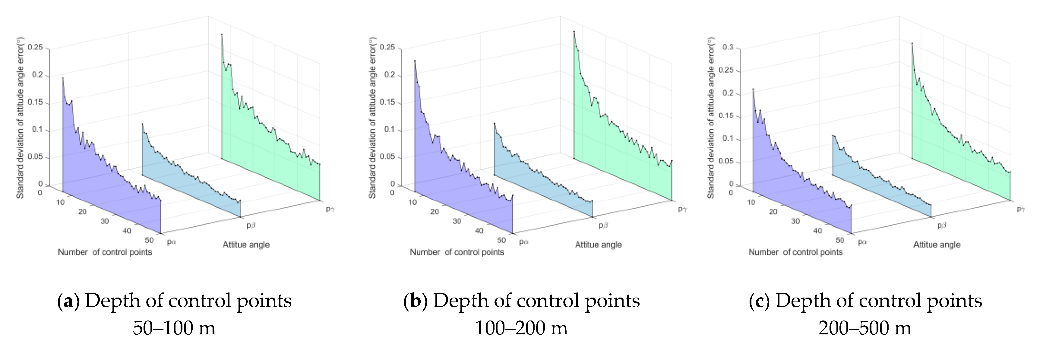
4.1. Performance with Respect to Number of Control Points

An experiment was conducted to evaluate the method’s accuracy with respect to a different number of control points, $n\in [6,50]$. The control points’ depths $o-x_c{y}_c{z}_c$ vary in the different ranges, i.e., 50–100, 100–200, and 200–500 m. Both the azimuth $\alpha$ and pitch $\beta$ are in the range $[20,70]$. Gaussian noise with 0 mean and standard deviation 0.05 ($°$) is added to azimuth $\alpha$ and pitch $\beta$. Gaussian noise with 0 mean and standard deviation 1.5 × 10⁻² (m) is added to control point $X_w={\left(x_w,y_w,z_w\right)}^T$. For each number of control points, 1000 independent trials were performed. The standard deviation of location error (SDLE) is the metric for location accuracy, and the standard deviation of attitude angle error (SDAAE) is the metric for attitude accuracy. The results are shown in Figure 12 and Figure 13, respectively. When the number of control points increases, both SDLE and SDAAE decrease. In case (a), when $n=40$, ${\sigma }_{p\alpha }=0.057°$, ${\sigma }_{p\beta }=0.029°$, ${\sigma }_{p\gamma }=0.062°$, ${\sigma }_x$= 0.22 m, ${\sigma }_y$ = 0.11 m, and ${\sigma }_z$ = 0.16 m.

4.2. Performance with Respect to Angle Noise Level

An experiment was conducted to evaluate the accuracy with respect to different angle noises. The number of control points is 50. The depth of the control points is 50–100, 100–200, and 200–500 m. Both azimuth $\alpha$ and pitch $\beta$ are in the range $[20,70]$. Gaussian noise with 0 mean and standard deviation ${\sigma }_{angle}\in [0.005,0.05]$ ($°$) is added to azimuth $\alpha$ and pitch $\beta$. Gaussian noise with mean 0 and standard deviation ${\sigma }_{3d}=1.5\times {10}^{{}^{-}2}$ (m) is added to the control point $X_w={\left(x_w,y_w,z_w\right)}^T$. For each noise level, 1000 independent trials were performed. The SDAAE and SDLE results are shown in Figure 14 and Figure 15, SDLE vs. angle noise ${\sigma }_{angle}$, respectively.

It can be seen from Figure 14 and Figure 15 that SDLE and SDAAE, respectively, both decrease with increasing ${\sigma }_{angle}$. In case (a), ${\sigma }_{angle}=0.05$, which is easy to carry out using the MVMS, and ${\sigma }_{p\alpha }=0.051°$, ${\sigma }_{p\beta }=0.024°$, ${\sigma }_{p\gamma }=0.054°$, ${\sigma }_x$= 0.17 m, ${\sigma }_y$ = 0.09 m, and ${\sigma }_z$= 0.13 m.

5. Conclusions

In this paper, a virtual omnidirectional camera model of the MVMS is established to globally calibrate the location and attitude in the field. Moreover, this model enlarges the distribution range of the control points in 3D space and improves the transforming accuracy from the turntable angles of azimuth and pitch to the virtual image coordinates in contrast to the virtual camera model with a virtual single image plane. Furthermore, an expanded factorial linear method is proposed to obtain the linear solutions of the location and attitude, which effectively restrains the measurement matrix errors from the angles of azimuth, pitch, and the control points. Finally, the location and attitude are transformed from the $o-x_g{y}_g{z}_g$ coordinate system to the $o-x_T{y}_T{z}_T$ coordinate system with the inherent geometric constraint of the tangent plane of the terrestrial sphere expressed by longitude and latitude. Simulations were conducted separately relating to the number of the control points and the noises of the turntable angles of azimuth and pitch to verify the accuracy and robustness of the method. In addition, an outdoor experiment was conducted to verify the accuracy and effectiveness of the proposed method.

References

1. Chai, B.; Liu, F.; Huang, Z.; Tan, K.; Wei, Z. An outdoor accuracy evaluation method of aircraft flight attitude dynamic vison measure system. In Proceedings of the Optical Sensing and Imaging Technologies and Applications, Beijing, China, 22–24 May 2018; p. 1084635. [Google Scholar]
2. Liu, Y.; Lin, J.R. Multi-sensor global calibration technology of vision sensor in car body-in-white visual measurement system. Acta Metrol. Sin. 2014, 5, 204–209. [Google Scholar]
3. Kitahara, I.; Saito, H.; Akimichi, S.; Onno, T.; Ohta, Y.; Kanade, T. Large-scale virtualized reality. In Proceedings of the IEEE Computer Vision & Pattern Recognition (CVPR), Technical Sketches, Kauai, HI, USA, 8–14 December 2001. [Google Scholar]
4. Cheng, J.H.; Ren, S.N.; Wang, G.L.; Yang, X.D.; Chen, K. Calibration and compensation to large-scale multi-robot motion platform using laser tracker. In Proceedings of the IEEE International Conference on Cyber Technology in Automation, Control, and Intelligent Systems (CYBER), Shenyang, China, 8–12 June 2015; pp. 163–168. [Google Scholar]
5. Liu, Z.; Li, F.J.; Zhang, G.J. An external parameter calibration method for multiple cameras based on laser rangefinder. Measurement 2014, 47, 954–962. [Google Scholar] [CrossRef]
6. Chen, G.; Guo, Y.; Wang, H.; Ye, D.; Gu, Y.J.O. Stereo vision sensor calibration based on random spatial points given by CMM. Optik 2012, 123, 731–734. [Google Scholar] [CrossRef]
7. Lu, R.S.; Li, Y.F. A global calibration method for large-scale multi-sensor visual measurement systems. Sens. Actuators A 2004, 116, 384–393. [Google Scholar] [CrossRef]
8. Zhao, Y.H.; Yuan, F.; Ding, Z.L.; Li, J. Global calibration method for multi-vision measurement system under the conditions of large field of view. J. Basic Sci. Eng. 2011, 19, 679–688. [Google Scholar]
9. Zhao, F.; Tamaki, T.; Kurita, T. Marker based simple non-overlapping camera calibration. In Proceedings of the IEEE International Conference on Image Processing (ICIP), Phoenix, AZ, USA, 25–28 September 2016; pp. 1180–1184. [Google Scholar]
10. Liu, Z.; Wei, X.G.; Zhang, G.J. External parameter calibration of widely distributed vision sensors with non-overlapping fields of view. Opt. Lasers Eng. 2013, 51, 643–650. [Google Scholar] [CrossRef]
11. Zou, W.; Li, S. Calibration of nonoverlapping in-vehicle cameras with laser pointers. IEEE Trans. Intell. Trans. Syst. 2015, 16, 1348–1359. [Google Scholar] [CrossRef]
12. Zou, W. Calibration Non-Overlapping Camera with a Laser Ray; Tottori University: Tottori, Japan, 2015. [Google Scholar]
13. Liu, Q.Z.; Sun, J.H.; Zhao, Y.T.; Liu, Z. Calibration method for geometry relationships of nonoverlapping cameras using light planes. Opt. Eng. 2013, 52. [Google Scholar] [CrossRef] [Green Version]
14. Liu, Q.; Sun, J.; Liu, Z.; Zhang, G. Global calibration method of multi-sensor vision system using skew laser lines. Chin. J. Mech. Eng. 2012, 25, 405–410. [Google Scholar] [CrossRef]
15. Nischt, M.; Swaminathan, R. Self-calibration of asynchronized camera networks. In Proceedings of the 2009 IEEE 12th International Conference on Computer Vision Workshops, ICCV Workshops, Kyoto, Japan, 27 September–4 October 2009; pp. 2164–2171. [Google Scholar]
16. Svoboda, T.J.E. Swiss Federal Institute of Technology, Zurich, Tech. Rep. BiWi-TR-263. Quick Guide to Multi-Camera Self-Calibration. 2003. Available online: http://www.vision.ee.ethz.ch/svoboda/SelfCal (accessed on 3 June 2020).
17. Kraynov, A.; Suchopar, A.; D’Souza, L.; Richards, R. Determination of geometric orientation of adsorbed cinchonidine on Pt and Fe and quiphos on Pt nanoclusters via DRIFTS. Phys. Chem. Chem. Phys. 2006, 8, 1321–1328. [Google Scholar] [CrossRef]
18. Khare, S.; Kodambaka, S.; Johnson, D.; Petrov, I.; Greene, J.J. Determining absolute orientation-dependent step energies: A general theory for the Wulff-construction and for anisotropic two-dimensional island shape fluctuations. Surf. Sci. 2003, 522, 75–83. [Google Scholar] [CrossRef]
19. Yu, F.; Xiong, Z.; Qu, Q. Multiple circle intersection-based celestial positioning and integrated navigation algorithm. J. Astronaut. 2011, 32, 88–92. [Google Scholar]
20. Yang, P.; Xie, L.; Liu, J. Simultaneous celestial positioning and orientation for the lunar rover. Aerosp. Sci. Technol. 2014, 34, 45–54. [Google Scholar] [CrossRef]
21. Meier, F.; Zakharchenya, B.P. Optical Orientation; Elsevier: Amsterdam, The Netherlands, 2012. [Google Scholar]
22. Bairi, A.J.S. Method of quick determination of the angle of slope and the orientation of solar collectors without a sun tracking system. Sol. Wind Technol. 1990, 7, 327–330. [Google Scholar] [CrossRef]
23. Lambrou, E.; Pantazis, G. Astronomical azimuth determination by the hour angle of Polaris using ordinary total stations. Surv. Rev. 2008, 40, 164–172. [Google Scholar] [CrossRef]
24. Ishikawa, T. Satellite navigation and geospatial awareness: Long-term effects of using navigation tools on wayfinding and spatial orientation. Prof. Geogr. 2019, 71, 197–209. [Google Scholar] [CrossRef]
25. Chen, Y.; Ding, X.; Huang, D.; Zhu, J. A multi-antenna GPS system for local area deformation monitoring. Earth Planets Space 2000, 52, 873–876. [Google Scholar] [CrossRef] [Green Version]
26. Bertiger, W.; Bar-Sever, Y.; Haines, B.; Iijima, B.; Lichten, S.; Lindqwister, U.; Mannucci, A.; Muellerschoen, R.; Munson, T.; Moore, A.W.; et al. A Real-Time Wide Area Differential GPS System. Navigation 1997, 44, 433–447. [Google Scholar] [CrossRef]
27. Bakuła, M.; Przestrzelski, P.; Kaźmierczak, R. Reliable technology of centimeter GPS/GLONASS surveying in forest environments. IEEE Trans. Geosci. Remote Sens. 2014, 53, 1029–1038. [Google Scholar] [CrossRef]
28. Siejka, Z.J.S. Validation of the accuracy and convergence time of real time kinematic results using a single galileo navigation system. Sensors 2018, 18, 2412. [Google Scholar] [CrossRef] [Green Version]
29. Specht, M.; Specht, C.; Wilk, A.; Koc, W.; Smolarek, L.; Czaplewski, K.; Karwowski, K.; Dąbrowski, P.S.; Skibicki, J.; Chrostowski, P.; et al. Testing the Positioning Accuracy of GNSS Solutions during the Tramway Track Mobile Satellite Measurements in Diverse Urban Signal Reception Conditions. Energies 2020, 13, 3646. [Google Scholar] [CrossRef]
30. Lai, L.; Wei, W.; Li, G.; Wu, D.; Zhao, Y. Design of Gimbal Control System for Miniature Control Moment Gyroscope. In Proceedings of the 2018 Chinese Automation Congress (CAC), Xi’an, China, 30 November–2 December 2018; pp. 3529–3533. [Google Scholar]
31. Belfi, J.; Beverini, N.; Bosi, F.; Carelli, G.; Cuccato, D.; De Luca, G.; Di Virgilio, A.; Gebauer, A.; Maccioni, E.; Ortolan, A.; et al. Deep underground rotation measurements: GINGERino ring laser gyroscope in Gran Sasso. Rev. Sci. Instrum. 2017, 88, 034502. [Google Scholar] [CrossRef] [PubMed] [Green Version]
32. Zhou, Z.; Tan, Z.; Wang, X.; Wang, Z. Experimental analysis of the dynamic north-finding method based on a fiber optic gyroscope. Appl. Opt. 2017, 56, 6504–6510. [Google Scholar] [CrossRef]
33. Liu, Y.; Shi, M.; Wang, X. Progress on atomic gyroscope. In Proceedings of the 2017 24th Saint Petersburg International Conference on Integrated Navigation Systems (ICINS), Saint Petersburg, Russia, 29–31 May 2017. [Google Scholar]
34. Schwartz, S.; Feugnet, G.; Morbieu, B.; El Badaoui, N.; Humbert, G.; Benabid, F.; Fsaifes, I.; Bretenaker, F. New approaches in optical rotation sensing. In Proceedings of the International Conference on Space Optics—ICSO 2014, Tenerife, Spain, 7–10 October 2014; p. 105633Y. [Google Scholar]
35. Kok, M.; Hol, J.D.; Schön, T.B. Using inertial sensors for position and orientation estimation. arXiv 2017, arXiv:1704.06053. [Google Scholar]
36. Krasuski, K.; Savchuk, S. Determination of the Precise Coordinates of the GPS Reference Station in of a GBAS System in the Air Transport. Commun. Sci. Lett. Univ. Zilina 2020, 22, 11–18. [Google Scholar] [CrossRef]
37. Paziewski, J.; Sieradzki, R.; Baryla, R. Multi-GNSS high-rate RTK, PPP and novel direct phase observation processing method: Application to precise dynamic displacement detection. Meas. Sci. Technol. 2018, 29, 035002. [Google Scholar] [CrossRef]
38. Wu, F.; Hu, Z.; Duan, F. 8-point algorithm revisited: Factorized 8-point algorithm. In Proceedings of the Tenth IEEE International Conference on Computer Vision (ICCV’05), Kyoto, Japan, 27 September–4 October 2009; Volume 1, pp. 488–494. [Google Scholar]
39. Li, Y. The Design and Implementation of Coordinate Conversion System; China University of Geosciences: Wuhan, China, 2010. [Google Scholar]
40. Yan, M.; Du, P.; Wang, H.-L.; Gao, X.-J.; Zhang, Z.; Liu, D. Ground multi-target positioning algorithm for airborne optoelectronic system. J. Appl. Opt. 2012, 33, 717–720. [Google Scholar]
Figure 1. Method flowchart.
Remotesensing 13 01982 g001
Figure 2. Virtual omnidirectional camera model of MVMS.
Remotesensing 13 01982 g002
Figure 3. Virtual imaging illustration in π z and π z .
Remotesensing 13 01982 g003
Figure 4. Virtual camera model on π z .
Remotesensing 13 01982 g004
Figure 5. Location and attitude transform.
Remotesensing 13 01982 g005
Figure 6. Inherent geometry constraint between o x T y T z T and o e x e y e z e .
Remotesensing 13 01982 g006
Figure 7. Δ X vs. azimuth α .
Remotesensing 13 01982 g007
Figure 8. Δ Y , α vs. azimuth α .
Remotesensing 13 01982 g008
Figure 9. Δ Y , β vs. azimuth β .
Remotesensing 13 01982 g009
Figure 10. MVMS in the field.
Remotesensing 13 01982 g010
Figure 11. RTK GPS in the field.
Remotesensing 13 01982 g011
Figure 12. SDAAE vs. number of control points.
Remotesensing 13 01982 g012
Figure 13. SDLE vs. number of control points.
Remotesensing 13 01982 g013
Figure 14. SDAAE vs. angle noise σ a n g l e .
Remotesensing 13 01982 g014
Figure 15. SDLE vs. angle noise σ a n g l e .
Remotesensing 13 01982 g015