Group Target Tracking Based on MS-MeMBer Filters

Abstract

This paper presents a new group target tracking method based on the standard multi-sensor multi-target multi-Bernoulli (MS-MeMBer) filter. In the prediction step, the group structure is used to constrain the movement of the constituent members within the respective groups. Specifically, the group of members is considered as an undirected random graph. Combined with the virtual leader-follower model, the motion equation of the members within groups is formulated. In the update step, the partitioning problem of multiple sensors is transformed into a multi-dimensional assignment (MDA) problem. Compared with the original two-step greedy partitioning mechanism, the MDA algorithm achieves better measurement partitions in group target tracking scenarios. To evaluate the performance of the proposed method, a simulation scenario including group splitting and merging is established. Results show that, compared with the standard MS-MeMBer filter, our method can effectively estimate the cardinality of members and groups at the cost of increasing computational load. The filtering accuracy of the proposed method outperforms that of the MS-MeMBer filter.

1. Introduction

Group targets [1] can be considered as the formation of cooperative members whose locations obey special structures, such as unmanned aerial vehicle (UAV) formations, vehicle convoys, and flocks of birds, which are densely distributed and maintain certain patterns of movement. For tracking such targets, if a standard point target tracking method e.g., [2] was adopted, performance degradation would occur. On the one hand, the high density of measurement may lead to complex computations by standard tracking methods. On the other hand, the interaction between the members within the group is ignored, which is not conducive for improving the tracking accuracy and stability. In general, there are mainly two methods for tracking group targets: The “holistic” tracking method based on the group shape and centroid [3,4,5,6], and the “internal” tracking method based on group structures [7,8,9].

It is difficult to establish a stable trajectory for densely clustered targets with poor measurement resolution and severe echo crossing. A “holistic” tracking strategy [3] has been proposed to handle such targets, which focuses on the group shape and centroid state instead of focusing on targets within the group. Similar to the extended target tracking method [10,11,12,13,14], this strategy models the group shape, such as the elliptical model [15], the random hypersurface model (RHM) [16], and the star-convex model [17].

Tracking members within the group is of great significance in certain cases. For instance, by estimating the members’ states, one can distinguish friendly objects from enemies or predict the intention of the groups. In a high-resolution sensor system, the measurements of different members within the group are located in different resolution units and maintain a special distribution structure. Modelling the group structure is the basis for tracking internal members. By combining the group structure with the member’s state, the integrity and stability of target tracking can be improved. Several models of group structures have been proposed and widely used, such as the virtual leader-follower model [7], the Markov random field (MRF) model [8], and the evolving network model [9].

The filter based on random finite set (RFS) [18] avoids the complicated data association process and introduces a complete theoretical framework for target tracking. In the single-sensor field, the probability hypothesis density (PHD) [19], multi-target multi-Bernoulli (MeMBer) [20], generalized labelled multi-Bernoulli (GLMB) filters [21], and their variants [22,23,24] for group target tracking have been proposed. Moreover, the multi-sensor PHD (MS-PHD) [25], multi-sensor MeMBer (MS-MeMBer) [26], and multi-sensor GLMB (MS-GLMB) filters [27] have shown promising performance in handling multi-sensor measurements. Besides, several particle filters [28,29,30] have been proposed to improve the accuracy of the target state estimation. However, very few “internal” tracking methods have been considered in the literature for multi-sensor RFS filtering.

The MS-MeMBer filter inherits the advantages of the multi-Bernoulli filters with straightforward particle implementations and state estimation [20]. Although it cannot obtain target trajectories, it has a lower computational cost than that of the labelled versions [27]. Inspired by the idea of [23], we propose a group target tracking method using the virtual leader–follower model and the MS-MeMBer filter. Specifically, in the prediction step of the MS-MeMBer filter, we consider the group of individuals as an undirected random graph. Furthermore, the motion equation of targets within groups is introduced, combined with the virtual leader–follower model. Then, in the update step, the partition of multi-sensor measurements is transformed into a multi-dimensional assignment (MDA) problem. Using the MDA algorithm proposed in [31], better measurement partitions can be achieved in conditions for tracking targets within groups.

The rest of this paper is organized as follows. Section 2 briefly reviews the RFS and the original MS-MeMBer filter. Section 3 describes the group target tracking method proposed in this paper. Simulation results are given in Section 4. Finally, discussions are given in Section 5.

2. Background

2.1. The Random Finite Set

In the random finite set (RFS), the number of elements is random and finite, and the elements themselves are random and unordered. Thus, in the multi-target tracking field, the multi-target state and the measurements of targets can be intuitively represented by the RFS. Some examples of RFSs with special distributions are given next.

A Bernoulli RFS ${\widehat{X}}^{(i)}$ has a probability $1-r^{(i)}$ of being empty, and a probability $r^{(i)}$ of being a singleton ${\widehat{X}}^{(i)}=\{\mathrm{x}\}$ whose element is distributed with a function $p^{(i)}(\mathrm{x})$. The probability density of a Bernoulli RFS is given by

$$\pi ({\widehat{X}}^{(i)})=\{\begin{array}{cc}1-r^{(i)},& {\widehat{X}}^{(i)}=\varnothing \\ r^{(i)}\cdot p^{(i)}(\mathrm{x}),& {\widehat{X}}^{(i)}=\{\mathrm{x}\}\end{array},$$

(1)

which can be simplified to $\pi =(r^{(i)},p^{(i)}(\mathrm{x}))$.

A Multi-Bernoulli RFS $X$ is a union of a fixed number of independent Bernoulli RFSs, i.e., $\mathrm{X}={\displaystyle \underset{i=1}{\overset{M}{\cup }}{\widehat{X}}^{(i)}}$. $M$ is the number of Bernoulli RFSs in $X$, and the probability density of a multi-Bernoulli RFS is given by

$$\pi (\{{\mathrm{x}}_1,\dots ,{\mathrm{x}}_n\})={\displaystyle \prod _{j=1}^M(1-r^{(j)}){\displaystyle \sum _{1\le i_1\ne \cdots \ne i_n\le M}{\displaystyle \prod _{j=1}^n\frac{r^{(i_j)}{p}^{(i_j)}({\mathrm{x}}_j)}{1-r^{(i_j)}}}}},$$

(2)

which can be further simplified to $\pi ={\{(r_{}^{(i)},p_{}^{(i)}(\mathrm{x}))\}}_{i=1}^M$.

2.2. The MS-MeMBer Filter

In the established MS-MeMBer filter [26], the multi-target state at time $k-1$ is modelled as a multi-Bernoulli RFS $X_{k-1|k-1}$ and characterized by a posterior density ${\pi }_{k-1|k-1}$. The target is observed by S sensors, which generate independent measurements. The MS-MeMBer filter aims to estimate the density ${\pi }_{k|k}$ of the RFS $X_{k|k}$ given the set of all the measurements up to time k. The measurement partition is finished in the update step. Therefore, the multi-target state can be obtained in a Bayesian recursion [32] via prediction and update:

$$\cdot \cdot \cdot \to {\pi }_{k-1|k-1}\stackrel{prediction}{\to }{\pi }_{k|k-1}\stackrel{update}{\to }{\pi }_{k|k}\to \cdot \cdot \cdot$$

We summarize each step in the following sections.

2.2.1. The Prediction Step

Consider a multi-Bernoulli RFS $X_{k-1|k-1}$ composed of $M_{k-1|k-1}$ independent Bernoulli RFSs. The density of $X_{k-1|k-1}$ is

$${\pi }_{k-1|k-1}={\{(r_{k-1|k-1}^{(i)},p_{k-1|k-1}^{(i)}(\mathrm{x}))\}}_{i=1}^{M_{k-1|k-1}},$$

(3)

where each $(r_{k-1|k-1}^{(i)},p_{k-1|k-1}^{(i)}(\mathrm{x}))$ represents the independent Bernoulli density with probability $r_{k-1|k-1}^{(i)}$ and distribution function $p_{k-1|k-1}^{(i)}(\mathrm{x})$. Intuitively, $r_{k-1|k-1}^{(i)}$ indicates how likely the i-th Bernoulli RFS in $X_{k-1|k-1}$ is generated by a true target and $p_{k-1|k-1}^{(i)}(\mathrm{x})$ describes the estimated current state $\mathrm{x}$ of the target [33]. Therefore, we can obtain the multi-target state estimation by calculating the corresponding multi-Bernoulli density.

Given the birth multi-Bernoulli RFS with density ${\pi }_{B,k}={\{(r_{B,k}^{(i)},p_{B,k}^{(i)}(\mathrm{x}))\}}_{i=1}^{M_{B,k}}$, the predicted density ${\pi }_{k|k-1}$ is also a multi-Bernoulli with

$${\pi }_{k|k-1}={\{(r_{s,k-1|k-1}^{(i)},p_{s,k-1|k-1}^{(i)}(\mathrm{x}))\}}_{i=1}^{M_{k-1|k-1}}\cup {\{(r_{B,k}^{(i)},p_{B,k}^{(i)}(\mathrm{x}))\}}_{i=1}^{M_{B,k}},$$

(4)

where $M_{B,k}$ is the number of birth Bernoulli RFSs.

Additionally, the survival Bernoulli density follows

$$r_{s,k|k-1}^{(i)}=r_{k-1|k-1}^{(i)}\langle p_{k-1|k-1}^{(i)},{\rho }_{sv}\rangle ,$$

(5)

$$p_{s,k|k-1}^{(i)}(\mathrm{x})=\frac{\langle f_{k|k-1}(\mathrm{x}|\cdot ),{\rho }_{sv}{p}_{k-1|k-1}^{(i)}\rangle }{\langle p_{k-1|k-1}^{(i)},{\rho }_{sv}\rangle },$$

(6)

where ${\rho }_{sv}(\mathrm{x})$ represents the probability that a target with state x can survive to the next moment and $\langle f_1(\mathrm{x}),f_2(\mathrm{x})\rangle ={\displaystyle \int f_1(\mathrm{x})\cdot f_2(\mathrm{x})d\mathrm{x}}$ is the inner product function. $f_{k|k-1}(\mathrm{x}|\xi )$ is the state transfer function at time k, given previous state $\xi$.

2.2.2. Multi-Sensor Measurement Partition

In the update step of the MS-MeMBer filter, multi-sensor measurement partitions need to be produced. Measurement partition aims to divide the multi-sensor measurement set into target-originated subsets, which can be employed to associate the predicted Bernoulli RFSs.

Given a multi-sensor measurement set $Z_{1:S,k}=\{Z_{1,k},\dots ,Z_{S,k}\}$, each $Z_{j,k}(1\le j\le S)$ contains all measurements from sensor j at time k. For a number of $M_{k|k-1}$ predicted Bernoulli RFSs, we define a partition of set $Z_{1:S,k}$ as $\mathrm{P}=\{W_{1:S}^{(\mathrm{P},0)},W_{1:S}^{(\mathrm{P},1)},\dots ,W_{1:S}^{(\mathrm{P},M_{k|k-1})}\}$, where

$${\displaystyle \underset{i=0}{\overset{M_{k|k-1}}{\cup }}{W}_{1:S}^{(\mathrm{P},i)}}=Z_{1:S,k},$$

(7)

$$W_{1:S}^{(\mathrm{P},i)}=\{W_1^{(\mathrm{P},i)},\dots ,W_S^{(\mathrm{P},i)}\},\forall 0\le i\le M_{k|k-1},$$

(8)

$$W_{1:S}^{(\mathrm{P},i)}\cap W_{1:S}^{(\mathrm{P},l)}=\varnothing ,\forall 0\le i\ne l\le M_{k|k-1},$$

(9)

In partition $\mathrm{P}$, each $W_{1:S}^{(\mathrm{P},i)}(i>0)$ denotes the measurement set of target i generated by all S sensors and $W_{1:S}^{(\mathrm{P},0)}$ is the clutter measurement set. Each $W_j^{(\mathrm{P},i)}(1\le j\le S,i>0)$ in (8) contains the measurement of target i generated by sensor j. $W_j^{(\mathrm{P},0)}(1\le j\le S)$ is the collection of all clutter measurements on sensor j.

$𝒫$ is defined as the collection of all possible measurement partitions P. Finally, we define the mapping function $T_{W_{1:S}^{(\mathrm{P},i)}}=\{(j,l)|z_j^l\in W_{1:S}^{(\mathrm{P},i)}\}$, where j is the sensor number and $z_j^l$ is the l-th measurement in set $Z_{j,k}$.

It is difficult to obtain the exact implementation of the MS-MeMBer filter because of the complexity of obtaining all the measurement partitions. Partitions with low scores can be ignored because they have little effect on the update step. For this, a two-step greedy partitioning mechanism is proposed in [25], which can obtain several high-scoring measurement partitions.

In the two-step greedy partitioning mechanism, the global problem to obtain $𝒫$ is decomposed into independent sub-problems. We consider a measurement partitioning process with four sensors and three predicted Bernoulli components. First, local optimal solutions are achieved for each Bernoulli component, as shown in Figure 1. $z_j^0$ indicates that there is no measurement of sensor j associated with the Bernoulli component. Second, local optimal solutions of each Bernoulli component are combined to obtain several high-scoring partitions, as seen in Figure 2. The empty set $\varnothing$ means that all the measurements of S sensors are not associated with the Bernoulli component.

2.2.3. The Update Step

Given the predicted multi-target density with

$${\pi }_{k|k-1}={\{(r_{k|k-1}^{(i)},p_{k|k-1}^{(i)}(\mathrm{x}))\}}_{i=1}^{M_{k|k-1}},$$

(10)

and the updated multi-target density ${\pi }_{k|k}$ can be approximately expressed as

$${\pi }_{k|k}=\underset{\mathrm{P}\in \mathcal{P}}{\cup }\underset{i=1}{\overset{M_{k|k-1}}{\cup }}\{(r_{k|k}^{(\mathrm{P},i)},p_{k|k}^{(\mathrm{P},i)}(\mathrm{x}))\},$$

(11)

where $M_{k|k-1}=M_{k-1|k-1}+M_{B,k}$. For a given partition $\mathrm{P}$ in set $𝒫$, we can get the updated Bernoulli density $(r_{k|k}^{(\mathrm{P},i)},p_{k|k}^{(\mathrm{P},i)}(\mathrm{x}))$ with

$$r_{k|k}^{(\mathrm{P},i)}=\{\begin{array}{cc}{\alpha }_{\mathrm{P}}\frac{r_{k|k-1}^{(i)}\langle p_{k|k-1}^{(i)},\gamma \rangle }{1-r_{k|k-1}^{(i)}+r_{k|k-1}^{(i)}\langle p_{k|k-1}^{(i)},\gamma \rangle },& W_{1:S}^{(\mathrm{P},i)}=\varnothing \\ {\alpha }_{\mathrm{P}},& W_{1:S}^{(\mathrm{P},i)}\ne \varnothing \end{array},$$

(12)

$$p_{k|k}^{(\mathrm{P},i)}(\mathrm{x})=\{\begin{array}{cc}\frac{p_{k|k-1}^{(i)}(\mathrm{x})\gamma (\mathrm{x})}{\langle p_{k|k-1}^{(i)},\gamma \rangle },& W_{1:S}^{(\mathrm{P},i)}=\varnothing \\ \frac{p_{k|k-1}^{(i)}(\mathrm{x})f(W_{1:S}^{(\mathrm{P},i)}|\mathrm{x})}{{\displaystyle \int p_{k|k-1}^{(i)}(\mathrm{x})f(W_{1:S}^{(\mathrm{P},i)}|\mathrm{x})d\mathrm{x}}},& W_{1:S}^{(\mathrm{P},i)}\ne \varnothing \end{array}.$$

(13)

As can be seen from (12) and (13), each updated Bernoulli component $(r_{k|k}^{(\mathrm{P},i)},p_{k|k}^{(\mathrm{P},i)}(\mathrm{x}))$ is obtained only by the corresponding set $W_{1:S}^{(\mathrm{P},i)}$. $\gamma (\mathrm{x})={\displaystyle {\prod }_{j=1}^S(1-p_{j,D}(\mathrm{x}))}$ is the probability that a target is detected by no sensor. $p_{j,D}(\mathrm{x})$ is the target detection probability of sensor j. $f(W_{1:S}^{(\mathrm{P},i)}|\mathrm{x})$ is the single-target multi-sensor likelihood function under clutter conditions, and follows

$$f(W_{1:S}^{(\mathrm{P},i)}|\mathrm{x})={\displaystyle \prod _{(j,l)\in T_{W_{1:S}^{(\mathrm{P},i)}}}\frac{p_{j,D}(\mathrm{x})g_j(z_j^l|\mathrm{x})}{c_j(z_j^l)}\cdot {\displaystyle \prod _{(j,*)\notin T_{W_{1:S}^{(\mathrm{P},i)}}}(1-p_{j,D}(\mathrm{x}))}}.$$

(14)

$g_j(\cdot |\mathrm{x})$ and $c_j(\cdot )$ are the measurement likelihood and the clutter density of sensor j, respectively.

The coefficient ${\alpha }_{\mathrm{P}}$ is given by

$${\alpha }_{\mathrm{P}}=\frac{K_{\mathrm{P}}{\displaystyle {\prod }_{i=1}^{M_{k|k-1}}}{\phi }_{W_{1:S}^{(\mathrm{P},i)}}^i\{1\}}{{\displaystyle \sum _{\mathrm{M}\in \mathcal{P}}}{K}_{\mathrm{M}}{\displaystyle {\prod }_{i=1}^{M_{k|k-1}}}{\phi }_{W_{1:S}^{(\mathrm{M},i)}}^i\{1\}},$$

(15)

where

$${\phi }_{W_{1:S}^{(\mathrm{P},i)}}^i[u]=\{\begin{array}{cc}1-r_{k|k-1}^{(i)}+r_{k|k-1}^{(i)}\langle p_{k|k-1}^{(i)},u\gamma \rangle ,& W_{1:S}^{(\mathrm{P},i)}=\varnothing \\ r_{k|k-1}^{(i)}{\displaystyle \int u(\mathrm{x})}{p}_{k|k-1}^{(i)}(\mathrm{x})f(W_{1:S}^{(\mathrm{P},i)}|\mathrm{x})d\mathrm{x},& W_{1:S}^{(\mathrm{P},i)}\ne \varnothing \end{array}.$$

(16)

In (15), ${\phi }_{W_{1:S}^{(\mathrm{P},i)}}^i\{1\}$ represents the value of function ${\phi }_{W_{1:S}^{(\mathrm{P},i)}}^i[u]$ evaluated at $u=1$. Intuitively, ${\phi }_{W_{1:S}^{(\mathrm{P},i)}}^i\{1\}$ scores the association of the measurement set $W_{1:S}^{(\mathrm{P},i)}$ with the i-th Bernoulli component $(r_{k|k-1}^{(i)},p_{k|k-1}^{(i)}(\mathrm{x}))$, while $K_{\mathrm{P}}{\displaystyle {\prod }_{i=1}^{M_{k|k-1}}{\phi }_{W_{1:S}^{(\mathrm{P},i)}}^i\{1\}}$ represents a score of the partition $\mathrm{P}$. ${\alpha }_{\mathrm{P}}$ represents the weight of $\mathrm{P}$ in collection $𝒫$, which can be calculated by dividing the score of $\mathrm{P}$ by the sum of all the partitioning scores in $𝒫$. $K_{\mathrm{P}}={\displaystyle {\prod }_{j=1}^S{C}_j{}^{(|W_j^{(\mathrm{P},0)}|)}}(0)$ denotes the constraint of the clutter set, where $\left|W_j^{(\mathrm{P},0)}\right|$ is the cardinality of set $W_j^{(\mathrm{P},0)}$, and $C_j{}^{(n)}(\cdot )$ is the n-th derivative of the clutter probability generating function.

3. The Group Target Tracking

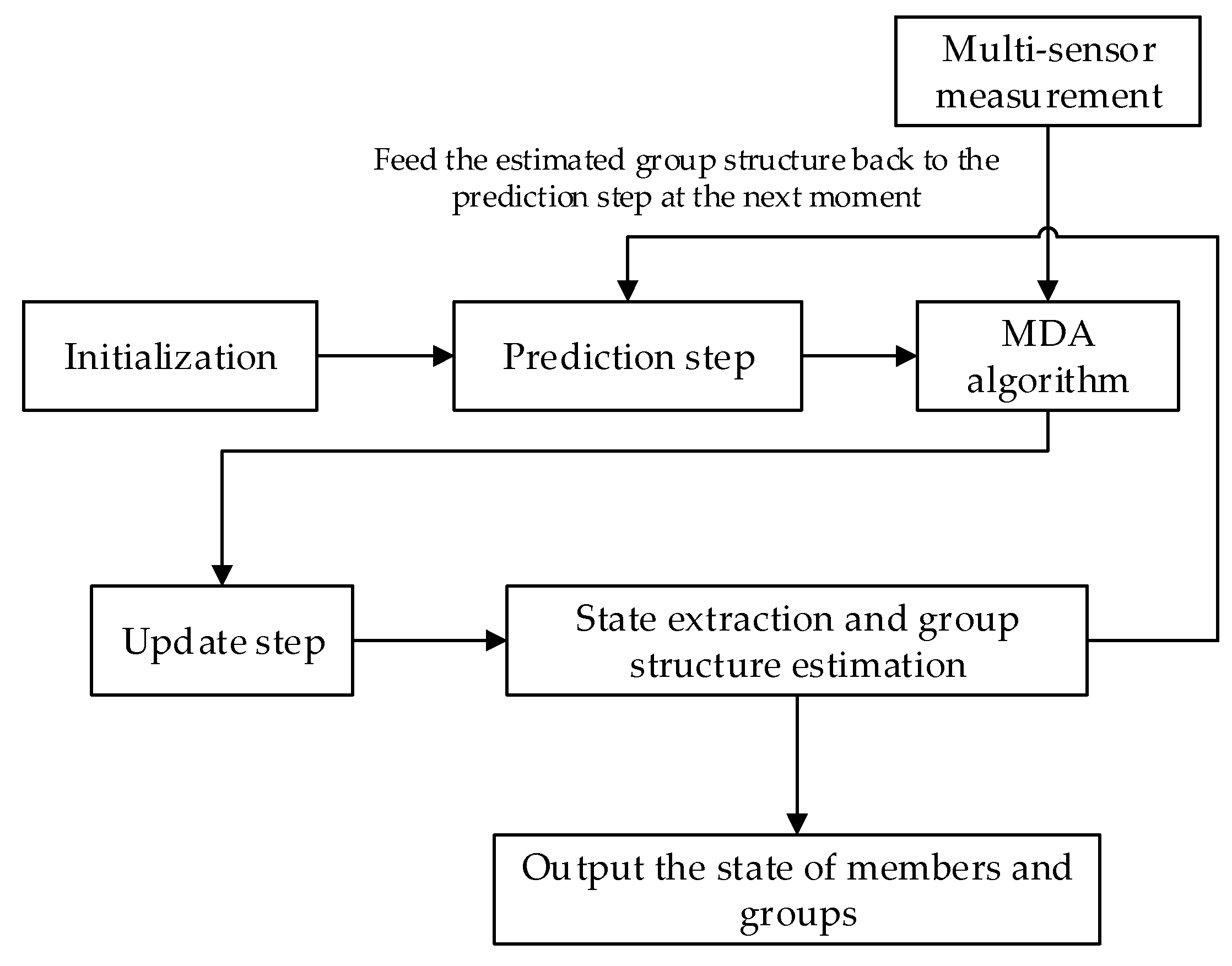
Based on the MS-MeMBer filter, a new group target tracking method is proposed. First, the filter parameters and the group structure are initialized according to the initial state of members. Then, in the prediction step, the movement of the members within a group is constrained by the group structure. Furthermore, in the update step, the partition of multi-sensor measurements is transformed into a multi-dimensional assignment (MDA) problem. Compared with the original two-step greedy partitioning mechanism [26], the MDA algorithm [31] can obtain better measurement partitions in group target tracking scenarios. Finally, the group structure is estimated through the current state of internal members and is fed back to the prediction step at the next moment. Also, the current state of members and groups is output. The flowchart of the proposed method is shown in Figure 3.

3.1. Graphical Representation of the Group

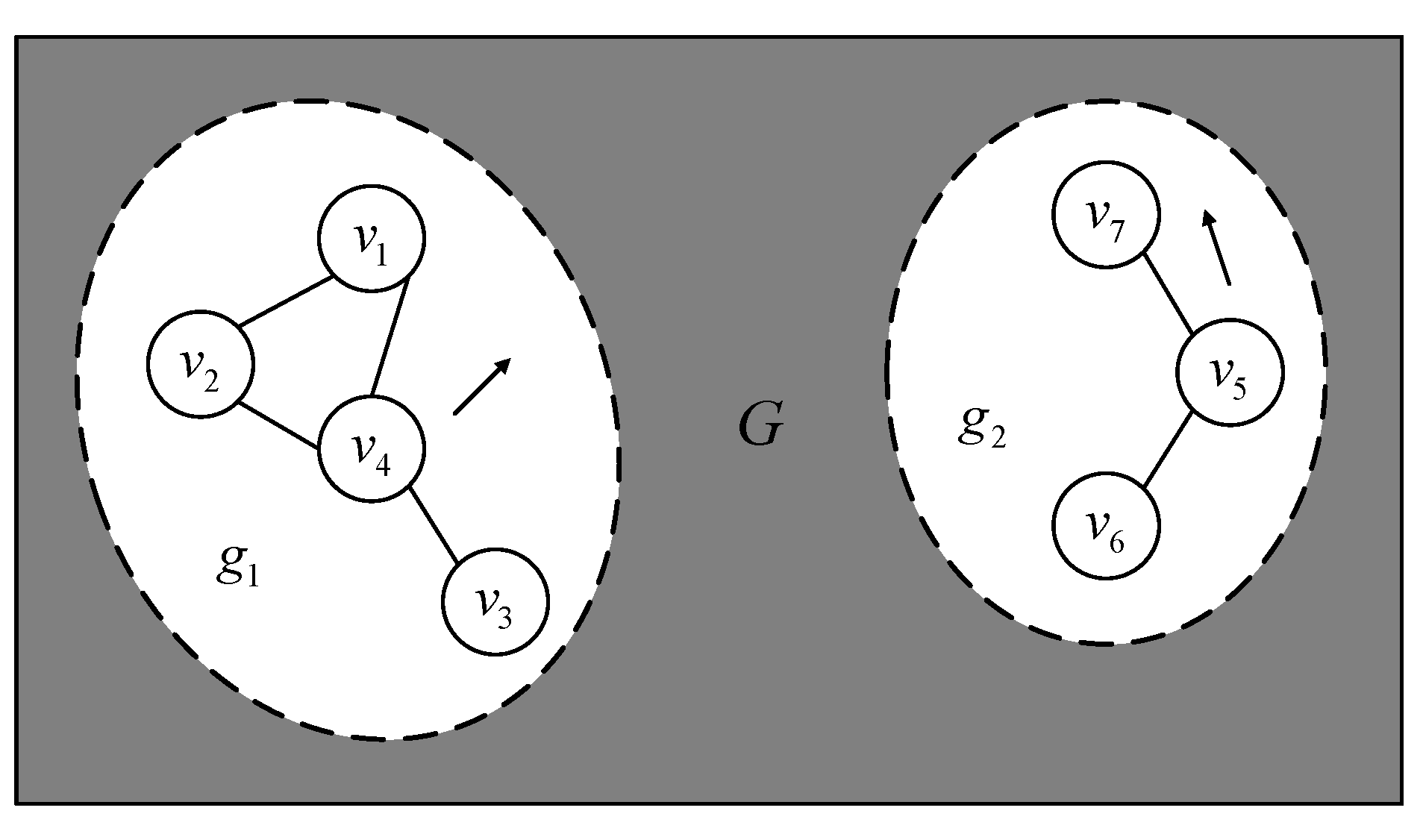
Graph theory [22] provides a convenient tool for describing groups, in which the relations between members are reflected by the edges between the related graph vertices. In this section, we consider the group of members as an undirected graph.

Given an undirected graph, $g_m=(V,E)$ of group m at time $k-1$. $V=(v_1,\dots ,v_n)$ is the vertex set composed of n individuals within group m, and each vertex $v_i$ contains the state and covariance of target i. For two different vertices $v_i$ and $v_j$, if the Mahalanobis distance $d_{ij}$ is less than the threshold $T_{\eta }$, it is determined that there is an edge connection between them. In other words, targets i and j are in the same group. $E$ is the collection of all edges between vertices in $V$. $\Gamma g(i)=\{j|j\ne i;v_i,v_j\in V\}$ is a mapping function that points to other members in the same group with target i. $G=(g_1,\dots ,g_m)$ represents a set of undirected graphs for each group. Figure 4 is a graphical representation of group targets, which shows seven moving targets belonging to two groups.

3.2. The System Model of Group Movement

The virtual leader–follower model [7] assumes that the state of any member is the translational offset of the group centroid. Consider a group with $n_g$ members at time $k-1$. We represent the member state as $\mathrm{x}={[p\mathrm{x},py,v\mathrm{x},vy]}^T$. $p\mathrm{x}$ and $py$ are the target positions. $v\mathrm{x}$ and $vy$ represent the target velocities along respective axes. According to the leader–follower model, the motion equation of the i-th member is given by

$$\begin{array}{ll}{\mathrm{x}}_{i,k}& ={\mathit{I}}_4{\mathrm{x}}_{i,k-1}+{\mathit{B}}_{k-1}\frac{1}{n_g}{\displaystyle \sum _{j=1}^{n_g}{\mathrm{x}}_{j,k-1}}+q_{i,k-1}\\ & ={\mathit{F}}_{k-1}{\mathrm{x}}_{i,k-1}+{\mathit{B}}_{k-1}{u}_{i,k-1}+q_{i,k-1}\end{array},$$

(17)

where

$$u_{i,k-1}={\displaystyle \sum _{j\in \Gamma g(i)}{\mathrm{x}}_{j,k-1}},$$

(18)

$${\mathit{F}}_{k-1}=\left[\begin{array}{cc}{\mathit{I}}_2& \mathit{C}\\ {\mathbf{0}}_2& {\mathit{I}}_2\end{array}\right],{\mathit{B}}_{k-1}=\left[\begin{array}{cc}{\mathbf{0}}_2& \mathit{C}\\ {\mathbf{0}}_2& {\mathbf{0}}_2\end{array}\right],\mathit{C}=\left[\begin{array}{cc}\frac{\Delta t}{n_g}& 0\\ 0& \frac{\Delta t}{n_g}\end{array}\right].$$

(19)

${\mathit{I}}_d$ and ${\mathbf{0}}_d$ are the unit matrix and zero matrix of size d, respectively. The process noise $q_{i,k-1}$ is considered as the zero-mean white Gaussian noise with variance ${\mathit{Q}}_{k-1}$. We can see from (17) that the movement of the members is not only related to its own state at the previous moment, but also restricted by other members in the same group. If $\Gamma g(i)$ is an empty set, then (17) can be simplified to the standard motion equation [2].

The observation equation of group members is given by

$$z_{i,k}={\mathit{H}}_k{\mathrm{x}}_{i,k}+r_{i,k},$$

(20)

where $z_{i,k}$ is the observation of ${\mathrm{x}}_{i,k}$, and $r_{i,k}$ is the measurement noise, which is usually assumed to be the zero-mean white Gaussian noise with variance ${\mathit{R}}_k$. ${\mathit{H}}_k$ is the observation matrix at time k.

3.3. Multi-Sensor Measurement Partition and MDA

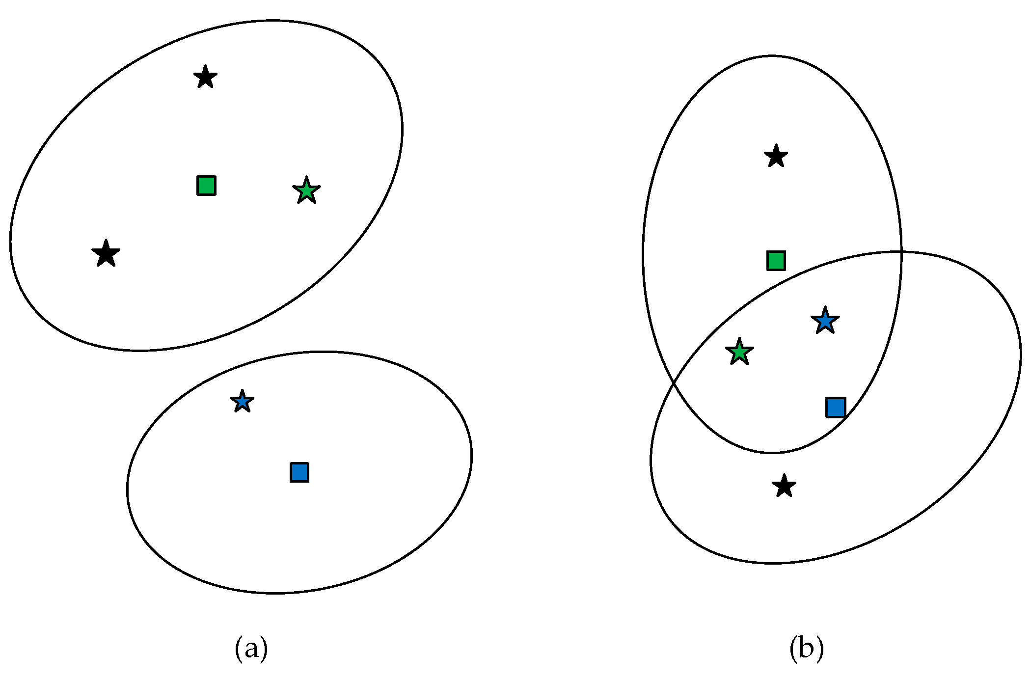
In the two-step greedy partitioning algorithm, each Bernoulli RFS (target) is assumed to be independent. Then, the target measurement set $W_{1:S}^{(P,i)}(i>0)$ of each Bernoulli RFS can be obtained separately. Also, the clutter measurement set $W_{1:S}^{(\mathrm{P},0)}$ is assumed to be independent of the target. Therefore, measurement partitions can be formed by combining each independent measurement set. As a divide-and-conquer strategy, this algorithm breaks the partitioning problem up into several independent sub-problems, which improves the efficiency of measurement partition. However, due to the dense distribution of individuals within groups, the association between measurements and targets is more complex. As can be seen from Figure 5, the measurement of a member would fall within the correlation threshold of other members in the same group. In this case, it is hard to maintain independence between the sub-problems in the two-step greedy partitioning mechanism. If the divide-and-conquer strategy is still adopted in group target tracking scenarios, the quality of the measurement partitions would deteriorate.

In this section, by eliminating the constraint of the clutter measurement set, the multi-sensor measurement partition can be interpreted as a multi-dimensional allocation problem, which can be solved by the MDA algorithm [27]. Compared with the two-step greedy partitioning mechanism, the MDA algorithm is implemented from the whole perspective, which improves the quality of multi-sensor measurement partitions. The derivation detail is given as follows.

From [25], the n-th derivative of function $C_j(\mathrm{x})$ obeys

$$C_j{}^{(n)}(\mathrm{x})={\lambda }_j{}^n{e}^{{\lambda }_j(\mathrm{x}-1)},$$

(21)

where ${\lambda }_j$ is the clutter intensity of sensor j.

Then the coefficient ${\alpha }_{\mathrm{P}}$ in (15) can be written as

$$\begin{array}{ll}{\alpha }_{\mathrm{P}}& =\frac{\frac{K_{\mathrm{P}}}{{\displaystyle {\prod }_{j=1}^S{C}_j{}^{(|Z_{j,k}|)}(0)}}\cdot {\displaystyle {\prod }_{i=1}^{M_{k|k-1}}{\phi }_{W_{1:S}^{(\mathrm{P},i)}}^i\{1\}}}{{\displaystyle \sum _{\mathrm{M}\in \mathcal{P}}}(\frac{K_{\mathrm{M}}}{{\displaystyle {\prod }_{j=1}^S{C}_j{}^{(|Z_{j,k}|)}(0)}}{\displaystyle {\prod }_{i=1}^{M_{k|k-1}}{\phi }_{W_{1:S}^{(\mathrm{M},i)}}^i\{1\})}}\\ & =\frac{\frac{1}{{\displaystyle {\prod }_{j=1}^S{\lambda }_j{}^{|Z_{j,k}\backslash W_j^{(\mathrm{P},0)}|}}}\cdot {\displaystyle {\prod }_{i=1}^{M_{k|k-1}}({\phi }_{W_{1:S}^{(\mathrm{P},i)}}^i\{1\})}}{{\displaystyle \sum _{\mathrm{M}\in \mathcal{P}}}(\frac{1}{{\displaystyle {\prod }_{j=1}^S{\lambda }_j{}^{|Z_{j,k}\backslash W_j^{(\mathrm{M},0)}|}}}\cdot {\displaystyle {\prod }_{i=1}^{M_{k|k-1}}{\phi }_{W_{1:S}^{(\mathrm{M},i)}}^i\{1\})}}\\ & =\frac{{\displaystyle {\prod }_{i=1}^{M_{k|k-1}}\left({\phi }_{W_{1:S}^{(\mathrm{P},i)}}^i\{1\}\cdot \frac{1}{{\displaystyle {\prod }_{j=1}^S{\lambda }_j{}^{\left|W_j^{(\mathrm{P},i)}\right|}}}\right)}}{{\displaystyle \sum _{\mathrm{M}\in \mathcal{P}}}{\displaystyle {\prod }_{i=1}^{M_{k|k-1}}\left({\phi }_{W_{1:S}^{(\mathrm{M},i)}}^i\{1\}\cdot \frac{1}{{\displaystyle {\prod }_{j=1}^S{\lambda }_j{}^{\left|W_j^{(\mathrm{M},i)}\right|}}}\right)}}\\ & =\frac{{\displaystyle {\prod }_{i=1}^{M_{k|k-1}}{\tilde{\phi }}_{W_{1:S}^{(\mathrm{P},i)}}^i\{1\}}}{{\displaystyle \sum _{\mathrm{M}\in \mathcal{P}}}{\displaystyle {\prod }_{i=1}^{M_{k|k-1}}{\tilde{\phi }}_{W_{1:S}^{(\mathrm{M},i)}}^i\{1\}}},\end{array}$$

(22)

where

$${\tilde{\phi }}_{W_{1:S}^{(\mathrm{P},i)}}^i\{1\}=\{\begin{array}{cc}1-r_{k|k-1}^{(i)}+r_{k|k-1}^{(i)}\langle p_{k|k-1}^{(i)},\gamma \rangle ,& W_{1:S}^{(\mathrm{P},i)}=\varnothing \\ r_{k|k-1}^{(i)}{\displaystyle \int p_{k|k-1}^{(i)}(\mathrm{x})\tilde{f}(W_{1:S}^{(\mathrm{P},i)}|\mathrm{x})d\mathrm{x}},& W_{1:S}^{(\mathrm{P},i)}\ne \varnothing \end{array},$$

(23)

$$\tilde{f}(W_{1:S}^{(\mathrm{P},i)}|\mathrm{x})={\displaystyle \prod _{(j,l)\in T_{W_{1:S}^{(\mathrm{P},i)}}}\frac{p_{j,D}(\mathrm{x})g_j(z_j^l|\mathrm{x})}{{\lambda }_{\mathrm{j}}{c}_j(z_j^l)}\cdot {\displaystyle \prod _{(j,*)\notin T_{W_{1:S}^{(\mathrm{P},i)}}}(1-p_{j,D}(\mathrm{x}))}}.$$

(24)

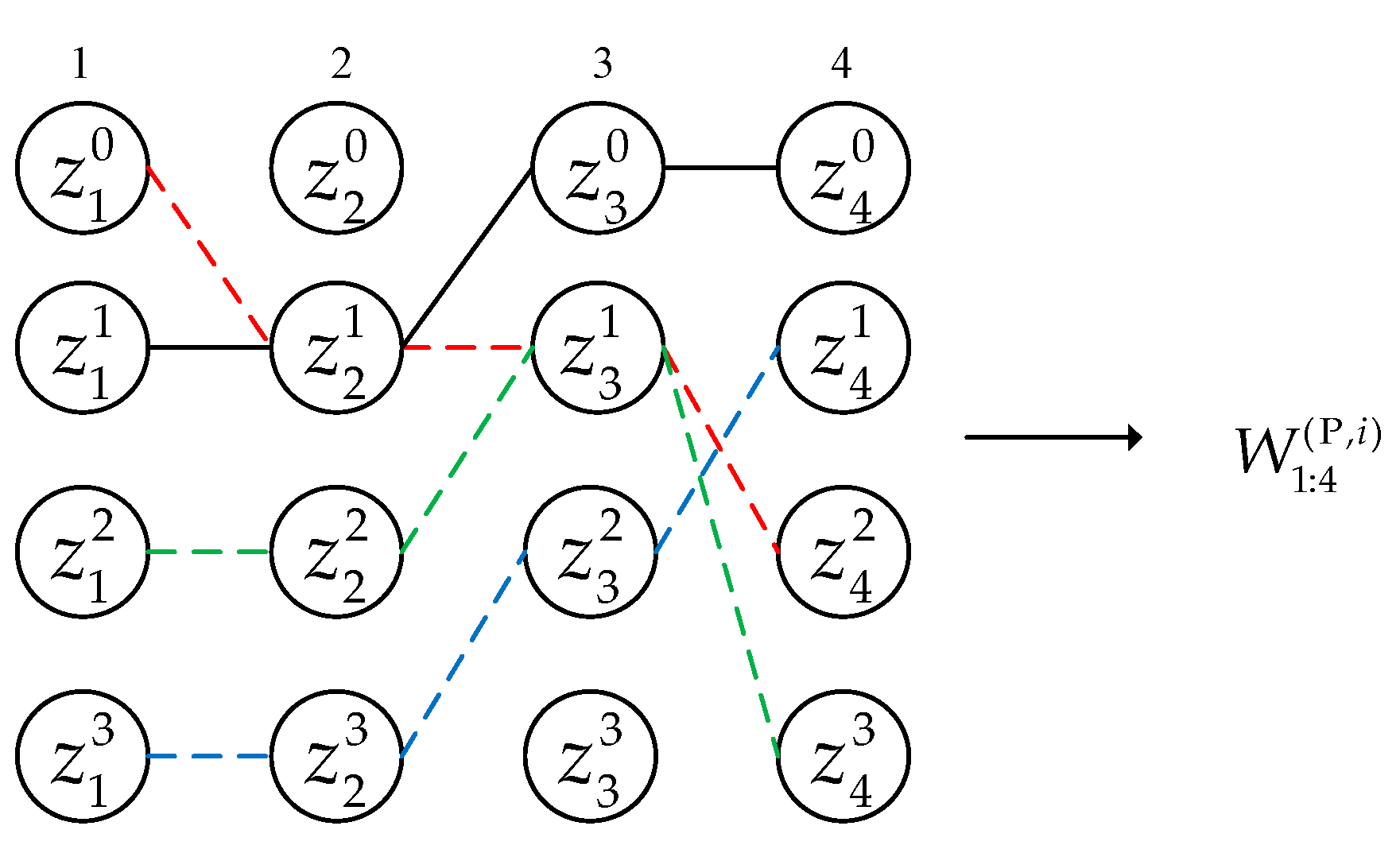
We employ ${\tilde{\phi }}_{W_{1:S}^{(\mathrm{P},i)}}^i\{1\}$ as a ratio of the likelihood that $W_{1:S}^{(\mathrm{P},i)}$ is generated by target i to the likelihood that $W_{1:S}^{(\mathrm{P},i)}$ is the clutter set. As can be seen from (22), the constraint of the clutter set $K_{\mathrm{P}}$ is eliminated. Therefore, we can obtain the partition $\mathrm{P}$ by associating $M_{k|k-1}$ Bernoulli RFSs with the measurements of S sensors.

In order to get the best association between multi-sensor measurements and Bernoulli components, the maximum score of $\mathrm{P}$ is required:

$$\underset{(W_{1:S}^{(\mathrm{P},1)},\dots ,W_{1:S}^{(\mathrm{P},M_{k|k-1})})}{\max }{\displaystyle {\prod }_{i=1}^{M_{k|k-1}}{\tilde{\phi }}_{W_{1:S}^{(\mathrm{P},i)}}^i\{1\}}.$$

(25)

The maximization problem shown in (25) is equivalent to the negative logarithmic minimization problem:

$$\begin{array}{ll}J& =\underset{(W_{1:S}^{(\mathrm{P},1)},\dots ,W_{1:S}^{(\mathrm{P},M_{k|k-1})})}{\min }{\displaystyle \sum _{i=1}^{M_{k|k-1}}-\ln ({\tilde{\phi }}_{W_{1:S}^{(\mathrm{P},i)}}^i\{1\})}\\ & =\underset{{\mu }_{j_1\cdots j_{S}i}}{\min }{\displaystyle \sum _{i=1}^{M_{k|k-1}}{\displaystyle \sum _{j_1=0}^{\left|Z_{1,k}\right|}\cdots {\displaystyle \sum _{j_S=0}^{\left|Z_{S,k}\right|}{c}_{j_1\cdots j_{S}i}{\mu }_{j_1\cdots j_{S}i}}}}\end{array}$$

(26)

where

$${\mu }_{j_1\cdots j_{S}i}=\{\begin{array}{cc}1,& W_{1:S}^{(\mathrm{P},i)}\subset Z_{1:S,k}\\ 0,& W_{1:S}^{(\mathrm{P},i)}\not\subset Z_{1:S,k}\end{array},$$

(27)

$$c_{j_1\cdots j_{S}i}=\{\begin{array}{cc}-\ln \left(1-r_{k|k-1}^{(i)}+r_{k|k-1}^{(i)}\langle p_{k|k-1}^{(i)},\gamma \rangle \right),& W_{1:S}^{(\mathrm{P},i)}=\varnothing \\ -\ln \left(r_{k|k-1}^{(i)}\right)-\ln \left({\displaystyle \int p_{k|k-1}^{(i)}(\mathrm{x})\tilde{f}(W_{1:S}^{(\mathrm{P},i)}|\mathrm{x})d\mathrm{x}}\right),& W_{1:S}^{(\mathrm{P},i)}\ne \varnothing \end{array}.$$

(28)

In (27), the decision variable ${\mu }_{j_1\cdots j_{S}i}=1$ denotes that the measurement set $W_{1:S}^{(\mathrm{P},i)}=\{z_1^{j_1},\dots ,z_S^{j_S}\}$ is associated with the i-th Bernoulli RFS. The number of predicted Bernoulli RFSs is given by $M_{k|k-1}$ and the number of measurements from sensor j at time k is $\left|Z_{j,k}\right|$. The constraint condition can be expressed as

$$\{\begin{array}{l}{\displaystyle \sum _{i=1}^{M_{k|k-1}}{\displaystyle \sum _{j_2=0}^{\left|Z_{2,k}\right|}\cdots {\displaystyle \sum _{j_S=0}^{\left|Z_{S,k}\right|}{\mu }_{j_1\cdots j_{S}i}=1,j_1=1,\dots ,\left|Z_{1,k}\right|}}}\hfill \\ {\displaystyle \sum _{i=1}^{M_{k|k-1}}{\displaystyle \sum _{j_1=0}^{\left|Z_{1,k}\right|}{\displaystyle \sum _{j_3=0}^{\left|Z_{3,k}\right|}\cdots {\displaystyle \sum _{j_S=0}^{\left|Z_{S,k}\right|}{\mu }_{j_1\cdots j_{S}i}=1,j_2=1,\dots ,\left|Z_{2,k}\right|}}}}\hfill \\ ⋮\\ {\displaystyle \sum _{i=1}^{M_{k|k-1}}{\displaystyle \sum _{j_1=0}^{\left|Z_{1,k}\right|}\cdots {\displaystyle \sum _{j_{S-1}=0}^{\left|Z_{S-1,k}\right|}{\mu }_{j_1\cdots j_{S}i}=1,j_S=1,\dots ,\left|Z_{S,k}\right|}}}\hfill \\ {\displaystyle \sum _{j_1=0}^{\left|Z_{1,k}\right|}\dots {\displaystyle \sum _{j_S=0}^{\left|Z_{S,k}\right|}{\mu }_{j_1\cdots j_{S}i}}=1,i=1,\dots ,M_{k|k-1}}\hfill \end{array},$$

(29)

which guarantees that two different Bernoulli RFSs cannot share the same real measurement, and that a Bernoulli RFS can be associated with an empty set $\varnothing$.

The minimization problem shown in (26) can be solved by the MDA algorithm [27]. Also, multiple high-scoring partitions are needed in the update step. Therefore, a list can be created that ranks feasible solutions in the order of cost factors.

3.4. Gaussian Mixture Implementation

It is very intractable to calculate multiple integrals in the prediction step and update step of the MS-MeMBer filter. Therefore, a Gaussian mixture (GM) implementation is adopted, in which the distribution function of each Bernoulli component is assumed to follow a GM form.

3.4.1. Prediction Step

Assume that at time $k-1$, the distribution function of each Bernoulli component has the following GM form:

$$p_{k-1|k-1}^{(i)}(\mathrm{x})={\displaystyle \sum _{n=1}^{J_{k-1|k-1}^{(i)}}{w}_{n,k-1|k-1}^{(i)}\mathcal{N}(\mathrm{x};{\mathit{m}}_{n,k-1|k-1}^{(i)},{\mathit{P}}_{n,k-1|k-1}^{(i)})},$$

(30)

where $\mathcal{N}(\mathrm{x};{\mathit{m}}_{n,k-1|k-1}^{(i)},{\mathit{P}}_{n,k-1|k-1}^{(i)})$ is a Gaussian function with mean ${\mathit{m}}_{n,k-1|k-1}^{(i)}$ and variance ${\mathit{P}}_{n,k-1|k-1}^{(i)}$. $J_{k-1|k-1}^{(i)}$ is the number of the Gaussian components. $w_{n,k-1|k-1}^{(i)}$ is the weight of the corresponding component.

Using (17), the transfer function $f_{k|k-1}({\mathrm{x}}_{i,k}|{\mathrm{x}}_{i,k-1})$ follows

$$f_{k|k-1}({\mathrm{x}}_{i,k}|{\mathrm{x}}_{i,k-1})=\mathcal{N}({\mathrm{x}}_{i,k};{\mathit{F}}_{k-1}{\mathrm{x}}_{i,k-1}+{\mathit{B}}_{k-1}{u}_{i,k-1},{\mathit{Q}}_{k-1}).$$

(31)

Define the target survival probability as ${\rho }_{sv}(\mathrm{x})={\rho }_{sv}$, and the distribution function of newborn targets as a GM form with $p_{B,k}^{(i)}(\mathrm{x})={\displaystyle \sum _{n=1}^{J_{B,k}^{(i)}}{w}_{B,n,k}^{(i)}\mathcal{N}(\mathrm{x};{\mathit{m}}_{B,n,k}^{(i)},{\mathit{P}}_{B,n,k}^{(i)})}$.Then the distribution function of each survival Bernoulli component also has a GM form:

$$p_{s,k|k-1}^{(i)}(\mathrm{x})={\displaystyle \sum _{n=1}^{J_{k-1|k-1}^{(i)}}{w}_{n,k-1|k-1}^{(i)}\mathcal{N}(\mathrm{x};{\mathit{m}}_{n,k|k-1}^{(i)},{\mathit{P}}_{n,k|k-1}^{(i)})},$$

(32)

where

$${\mathit{m}}_{n,k|k-1}^{(i)}={\mathit{F}}_{k-1}{\mathit{m}}_{n,k-1|k-1}^{(i)}+{\mathit{B}}_{k-1}{u}_{i,k-1},$$

(33)

$${\mathit{P}}_{n,k|k-1}^{(i)}={\mathit{F}}_{k-1}{\mathit{P}}_{n,k-1|k-1}^{(i)}{\mathit{F}}_{k-1}{}^T+{\mathit{Q}}_{k-1}.$$

(34)

Furthermore, the probability $r_{s,k|k-1}^{(i)}$ of each survival Bernoulli follows

$$r_{s,k|k-1}^{(i)}=r_{k-1|k-1}^{(i)}{\rho }_{sv}.$$

(35)

3.4.2. Update Step

Assume that the distribution of each predicted Bernoulli component has the following GM form:

$$p_{k|k-1}^{(i)}(\mathrm{x})={\displaystyle \sum _{n=1}^{J_{k|k-1}^{(i)}}{w}_{n,k|k-1}^{(i)}\mathcal{N}(\mathrm{x};{\mathit{m}}_{n,k|k-1}^{(i)},{\mathit{P}}_{n,k|k-1}^{(i)})}.$$

(36)

Given the measurement likelihood function of each sensor $g_j(\cdot |\mathrm{x})=\mathcal{N}(\cdot ;{\mathit{H}}_k\mathrm{x},{\mathit{R}}_k)$, and the detection probability of each sensor $p_{j,D}(\mathrm{x})=p_{j,D}$, the distribution function of each updated Bernoulli component also has a GM form:

$$p_{k|k}^{(\mathrm{P},i)}(\mathrm{x})={\displaystyle \sum _{n=1}^{J_{k|k-1}^{(i)}}{w}_{n,k|k}^{(\mathrm{P},i)}\mathcal{N}(\mathrm{x};{\mathit{m}}_{n,k|k}^{(\mathrm{P},i)},{\mathit{P}}_{n,k|k}^{(\mathrm{P},i)})},$$

(37)

where

$$w_{n,k|k}^{(\mathrm{P},i)}=\{\begin{array}{c}\frac{w_{n,k|k-1}^{(i)}}{{\displaystyle \sum _{m=1}^{J_{k|k-1}^{(i)}}{w}_{m,k|k-1}^{(i)}}},W_{1:S}^{(\mathrm{P},i)}=\varnothing \\ \frac{w_{n,k|k-1}^{(i)}{\displaystyle \prod _{(j,l)\in T_{W_{1:S}^{(\mathrm{P},i)}}}\frac{p_{j,D}{q}_z(z_j^l)}{{\lambda }_{\mathrm{j}}{c}_j(z_j^l)}\cdot {\displaystyle \prod _{(j,*)\notin T_{W_{1:S}^{(\mathrm{P},i)}}}(1-p_{j,D})}}}{{\displaystyle \sum _{m=1}^{J_{k|k-1}^{(i)}}\left(w_{n,k|k-1}^{(i)}{\displaystyle \prod _{(j,l)\in T_{W_{1:S}^{(\mathrm{P},i)}}}\frac{p_{j,D}{q}_z(z_j^l)}{{\lambda }_{\mathrm{j}}{c}_j(z_j^l)}\cdot {\displaystyle \prod _{(j,*)\notin T_{W_{1:S}^{(\mathrm{P},i)}}}(1-p_{j,D})}}\right)}},W_{1:S}^{(\mathrm{P},i)}\ne \varnothing \end{array},$$

(38)

$$q_z(z_j^l)=\mathcal{N}(z_j^l;{\mathit{m}}_{n,k|k-1}^{(i)},{\mathit{R}}_k+{\mathit{H}}_k{\mathit{P}}_{n,k|k-1}^{(i)}{\mathit{H}}_k{}^T),$$

(39)

and

$$\mathcal{N}(\mathrm{x};{\mathit{m}}_{n,k|k}^{(\mathrm{P},i)},{\mathit{P}}_{n,k|k}^{(\mathrm{P},i)})\propto \{\begin{array}{cc}\mathcal{N}(\mathrm{x};{\mathit{m}}_{n,k|k-1}^{(i)},{\mathit{P}}_{n,k|k-1}^{(i)}),& W_{1:S}^{(\mathrm{P},i)}=\varnothing \\ \mathcal{N}(\mathrm{x};{\mathit{m}}_{n,k|k-1}^{(i)},{\mathit{P}}_{n,k|k-1}^{(i)})\cdot {\displaystyle \prod _{(j,l)\in T_{W_{1:S}^{(\mathrm{P},i)}}}{g}_j(z_j^l|\mathrm{x})},& W_{1:S}^{(\mathrm{P},i)}\ne \varnothing \end{array},$$

(40)

The updated probability $r_{k|k}^{(\mathrm{P},i)}$ satisfies

$$r_{k|k}^{(\mathrm{P},i)}=\{\begin{array}{cc}{\alpha }_{\mathrm{P}}\frac{r_{k|k-1}^{(i)}{\displaystyle \sum _{n=1}^{J_{k|k-1}^{(i)}}{\displaystyle {\prod }_{j=1}^S(1-p_{j,D})w_{n,k|k-1}^{(i)}}}}{1-r_{k|k-1}^{(i)}+r_{k|k-1}^{(i)}{\displaystyle \sum _{n=1}^{J_{k|k-1}^{(i)}}{\displaystyle {\prod }_{j=1}^S(1-p_{j,D})w_{n,k|k-1}^{(i)}}}},& W_{1:S}^{(\mathrm{P},i)}=\varnothing \\ {\alpha }_{\mathrm{P}},& W_{1:S}^{(\mathrm{P},i)}\ne \varnothing \end{array},$$

(41)

3.5. The State Extraction and Group Structure Estimation

The state extraction [25] is adopted to calculate the movement of all the targets, where the mean value is obtained from the densities of the updated Bernoulli RFSs with the exiting probabilities exceeding a given threshold. Consider the multi-target movement ${\{({\mathrm{x}}_{i,k},{\Sigma }_{i,k})\}}_{i=1}^n$ at time k, where ${\mathrm{x}}_{i,k}$ and ${\Sigma }_{i,k}$ are the kinematic state and covariance matrix of member i, respectively.

Suppose that at time k, the adjacency matrix is given by

$$D_k=\left[\begin{array}{cccc}0& {\eta }_k(1,2)& \cdots & {\eta }_k(1,n)\\ {\eta }_k(2,1)& 0& \cdots & {\eta }_k(2,n)\\ ⋮& ⋮& \ddots & ⋮\\ {\eta }_k(n,1)& {\eta }_k(n,2)& \cdots & 0\end{array}\right],$$

(42)

where

$${\eta }_k(i,j)=\{\begin{array}{cc}1,\hfill & \hfill d_{ij}<T_{\eta },i\ne j\\ 0,\hfill & \hfill others\end{array},$$

(43)

$$d_{ij}=\sqrt{({\mathrm{x}}_{i,k}-{\mathrm{x}}_{j,k}){({\Sigma }_{i,k}+{\Sigma }_{j,k})}^{-1}{({\mathrm{x}}_{i,k}-{\mathrm{x}}_{j,k})}^T}.$$

(44)

The structure and number of groups can be obtained by the adjacency matrix [23]. If the Mahalanobis distance between two targets is less than the threshold $T_{\eta }$, the two targets can be determined to be in the same group, and the corresponding value in the adjacency matrix is equal to one. For instance, the adjacency matrix of group 1 in Figure 4 can be denoted by

$$D=\left[\begin{array}{cccc}0& 1& 0& 1\\ 1& 0& 0& 1\\ 0& 0& 0& 1\\ 1& 1& 1& 0\end{array}\right].$$

(45)

Furthermore, the estimated group structure can be fed to the next step to update the state of members within the group.

4. Simulation Results

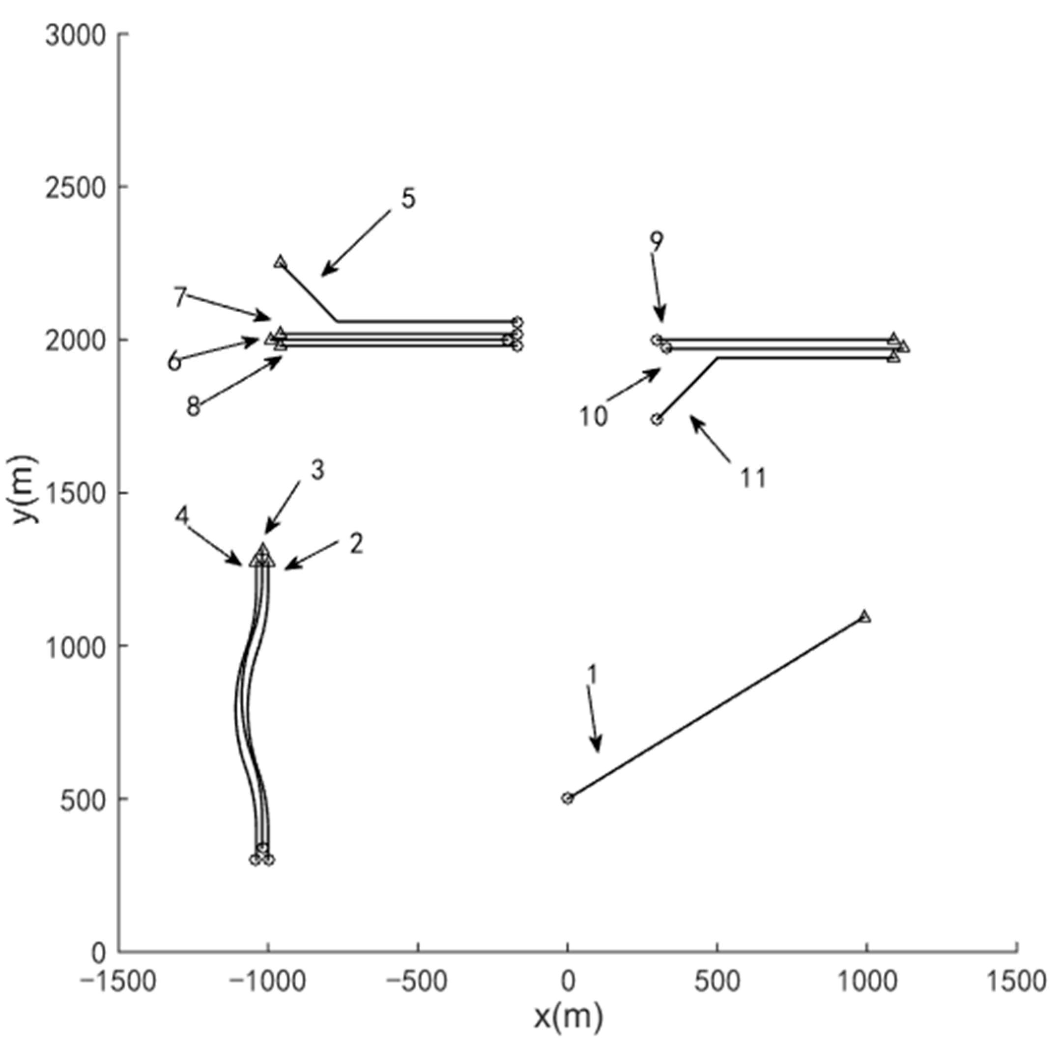
In this section, a two-dimensional area with size [−1500 m, 1500 m] × [0 m, 3000 m] is considered. Suppose that group targets that involve three subgroups moving in x-y plane. To verify the capability of the proposed method for tracking standard point targets, a single target in consistent velocity (CV) style is also considered. As shown in Figure 6, 11 moving targets are simulated. Among them, target 1 moves independently; target 2, target 3, and target 4 constitute group 1; target 5, target 6, target 7, and target 8 constitute group 2. Besides, target 5 separates from group 2 at about 65 s; target 9 and target 10 constitute group 3, and target 11 merges with this group at about 40 s. The kinematic parameters of targets are shown in

Table 1. The true movement of targets.

Target Number	Initial State	Survival Time
1	[0 m, 500 m, 10 m/s, 6 m/s]	(1 s–100 s)
2	[−1000 m, 300 m, 0 m/s, 10 m/s]	(1 s–100 s)
3	[−1040 m, 300 m, 0 m/s, 10 m/s]	(1 s–100 s)
4	[−1020 m, 340 m, 0 m/s, 10 m/s]	(1 s–100 s)
5	[−170 m, 2060 m, −10 m/s, 0 m/s]	(1 s–80 s)
6	[−200 m, 2000 m, −10 m/s, 0 m/s]	(1 s–80 s)
7	[−170 m, 2020 m, −10 m/s, 0 m/s]	(1 s–80 s)
8	[−170 m, 1080 m, −10 m/s, 0 m/s]	(1 s–80 s)
9	[300 m, 2000 m, 10 m/s, 0 m/s]	(21 s–100 s)
10	[330 m, 1070 m, 10 m/s, 0 m/s]	(21 s–100 s)
11	[300 m, 1740 m, 10 m/s, 10 m/s]	(21 s–100 s)

.

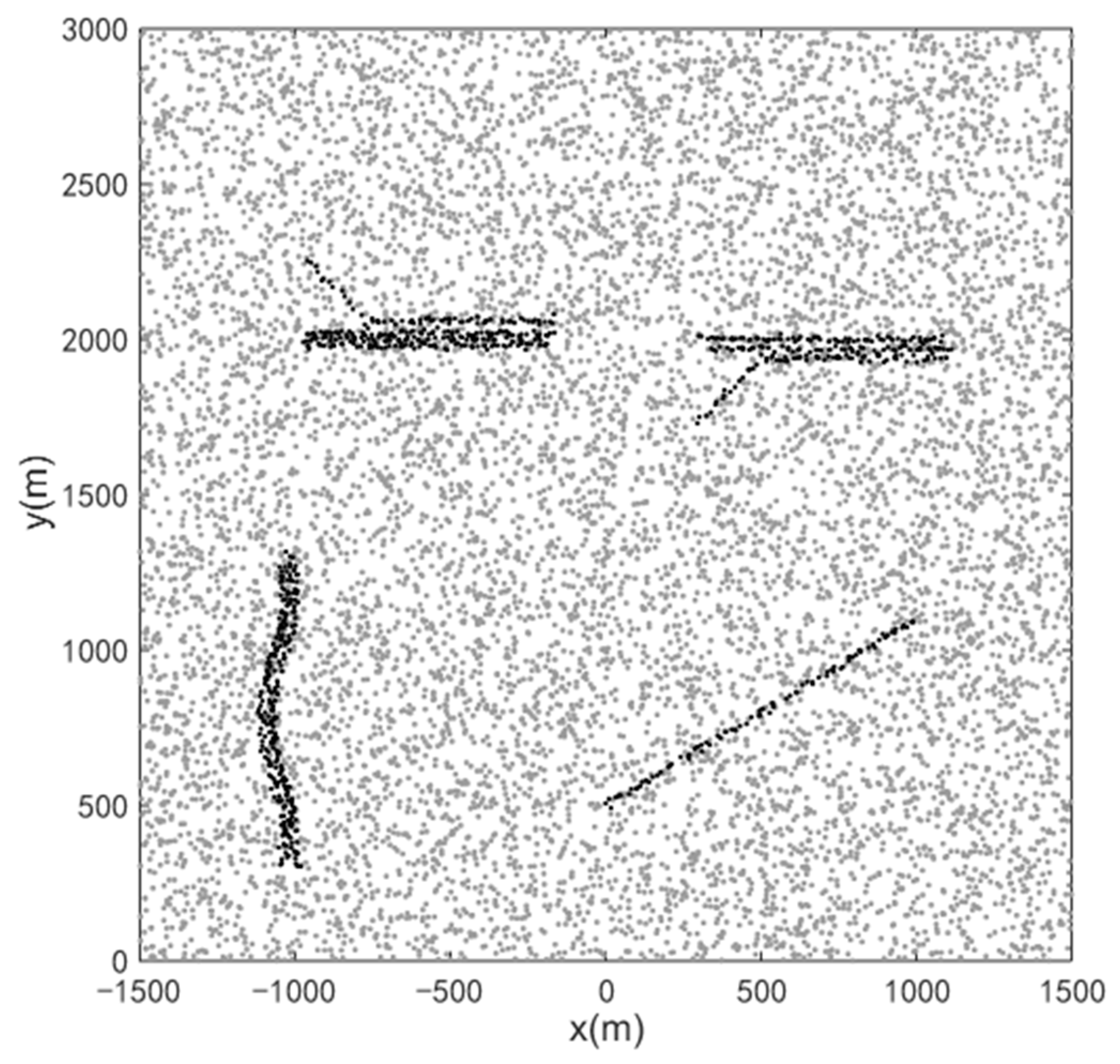
The duration time is 100 s, and the sampling period $\Delta t=1\mathrm{s}$. There are three sensors in the observation area. Figure 7 shows the measurements collected from sensor 1. The detection probability of each sensor is $p_{j,D}=0.85$, and the clutter intensity is ${\lambda }_j=100$. The birth model is set according to the initial state of the targets. The target survival probability is set as ${\rho }_{sv}=0.99$. The process noise covariance matrix ${\mathit{Q}}_k$, and the observation noise covariance matrix ${\mathit{R}}_k$ are respectively:

$${\mathit{Q}}_k=\left[\begin{array}{cc}\frac{\Delta t^3}{3}{\mathit{I}}_2& \frac{\Delta t^2}{2}{\mathit{I}}_2\\ \frac{\Delta t^2}{2}{\mathit{I}}_2& \Delta t{\mathit{I}}_2\end{array}\right]{\sigma }_v{}^2,{\mathit{R}}_k=\left[\begin{array}{cc}{\sigma }_{\epsilon }{}^2& 0\\ 0& {\sigma }_{\epsilon }{}^2\end{array}\right].$$

(46)

where ${\sigma }_v=3 \mathrm{m}/\mathrm{s}$ and ${\sigma }_{\epsilon }=6 \mathrm{m}$.

In the simulation, the number of the Bernoulli components is not more than $M_{\max }=100$, the number of the Gaussian components per target is not more than $J_{\max }=100$. The pruning threshold is set as $T_{\max }={10}^{-3}$. There are at most four measurement partitioning hypotheses in the set $𝒫$, and the number of the measurement subsets in each hypothesis $\mathrm{P}$ is up to $W_{\max }=4$. In addition, the Mahalanobis distance threshold is $T_{\eta }=15$. The simulation is performed using algorithms implemented in MATLAB on computers with one Intel Core i7-6700 CPU and 16 GB RAM. The average result is obtained through 50 Monte Carlo runs. The filtering performance is measured by the optimal sub-pattern assignment (OSPA) distance [34]. The OSPA distance accounts for both errors in estimation of target states and errors in estimation of target cardinality, where we set order $p=1$ and the penalty factor $c=100$.

As can be seen from Figure 8, in the group target tracking scenario, the OPSA error of the MS-MeMBer filter with group structure estimation is significantly smaller than that of the original MS-MeMBer filter. This means that the filtering accuracy is improved by using the group structure. In addition, compared with the above two methods, the proposed method with both the MDA algorithm and group structure estimation has the optimal filtering performance. Note that there is a peak of the OSPA error at about 80 s. This is because the filters mentioned above react slower to the death of the members.

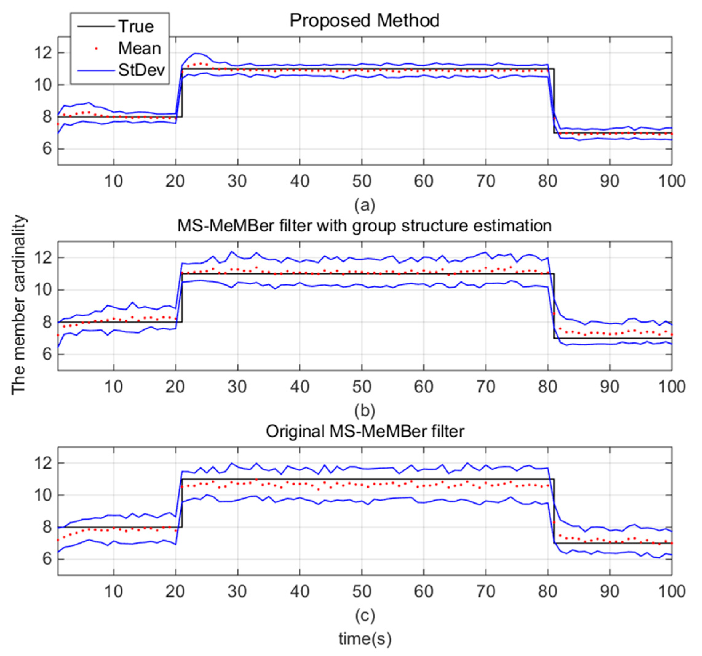
Figure 9 shows the members’ cardinality estimation of the above methods. The black line is the true cardinality of the members, the red dot is the estimated cardinality at the corresponding time, and the blue line represents the standard deviation of the estimated cardinality. We can see that for group target tracking, a cardinality estimation bias occurs in the original MS-MeMBer filter, which can be eliminated by using the group structure. Moreover, the standard deviation of cardinality estimation is further reduced by the MDA algorithm.

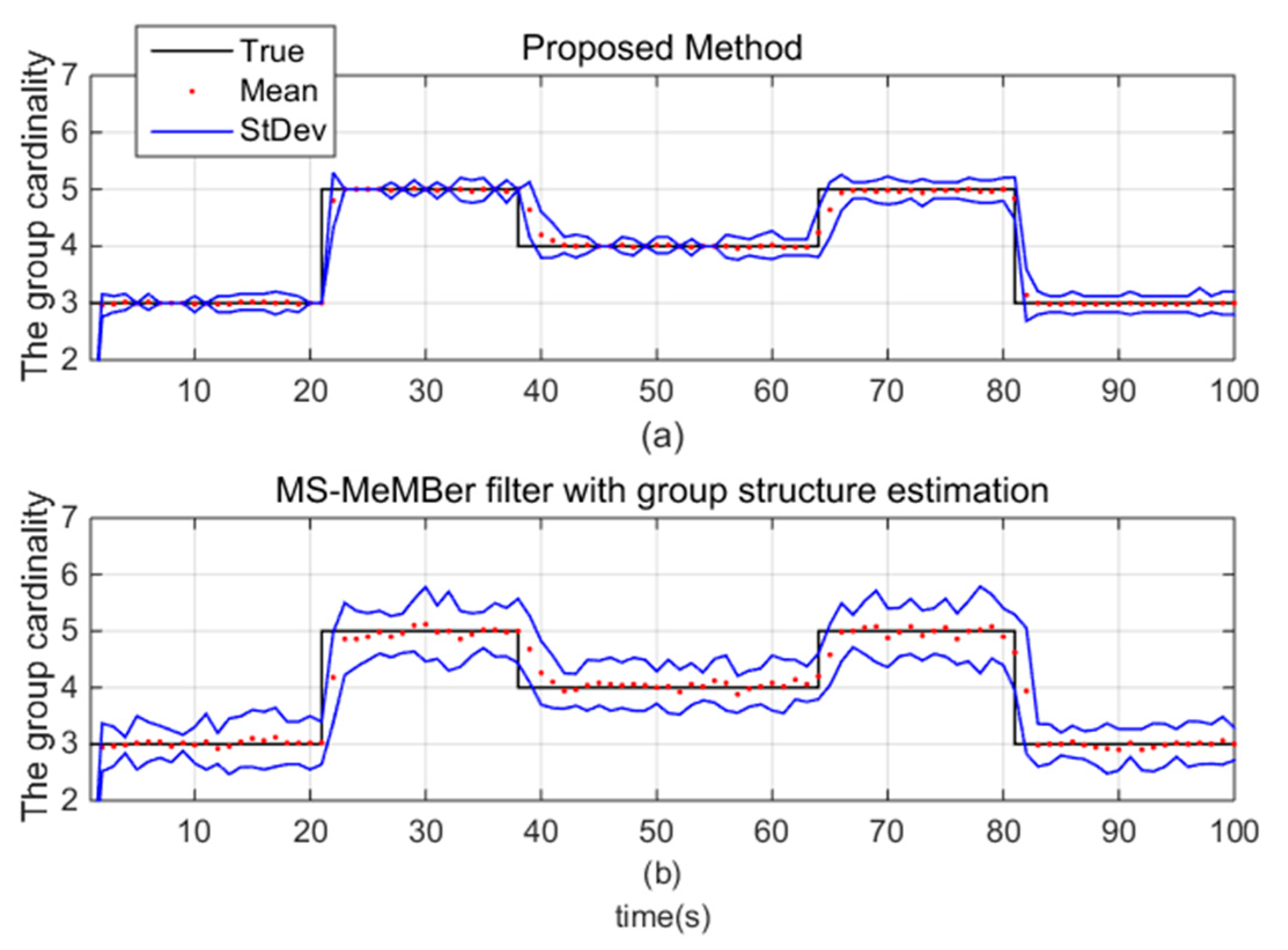
Figure 10 shows the estimated group cardinality of the proposed method. It can be seen that the proposed method obtains smaller standard deviations of the estimated group cardinality. We can conclude that compared with the MS-MeMBer filter, which only contains the group structure estimation, the proposed method with both group structure estimation and MDA algorithm obtains better estimation of the group cardinality.

Table 2. Average running time.

The Total Number of Sensors	Running Time of the Proposed Method	Running Time of the MS-MeMBer Filter
3	4.55 s	5.84 s
4	9.36 s	6.41 s
5	27.08 s	7.78 s

shows the average running time of the MS-MeMBer filter and the proposed method in scenarios with different number of sensors. The number of the sensors is varied in the range {3, 4, 5}. By comparison, they have similar time consumptions when the number of the sensors is small. However, the computational complexity of the MDA algorithm increases exponentially with the increasing number of the sensors, leading to a significant increase in the time consumption of the proposed method.

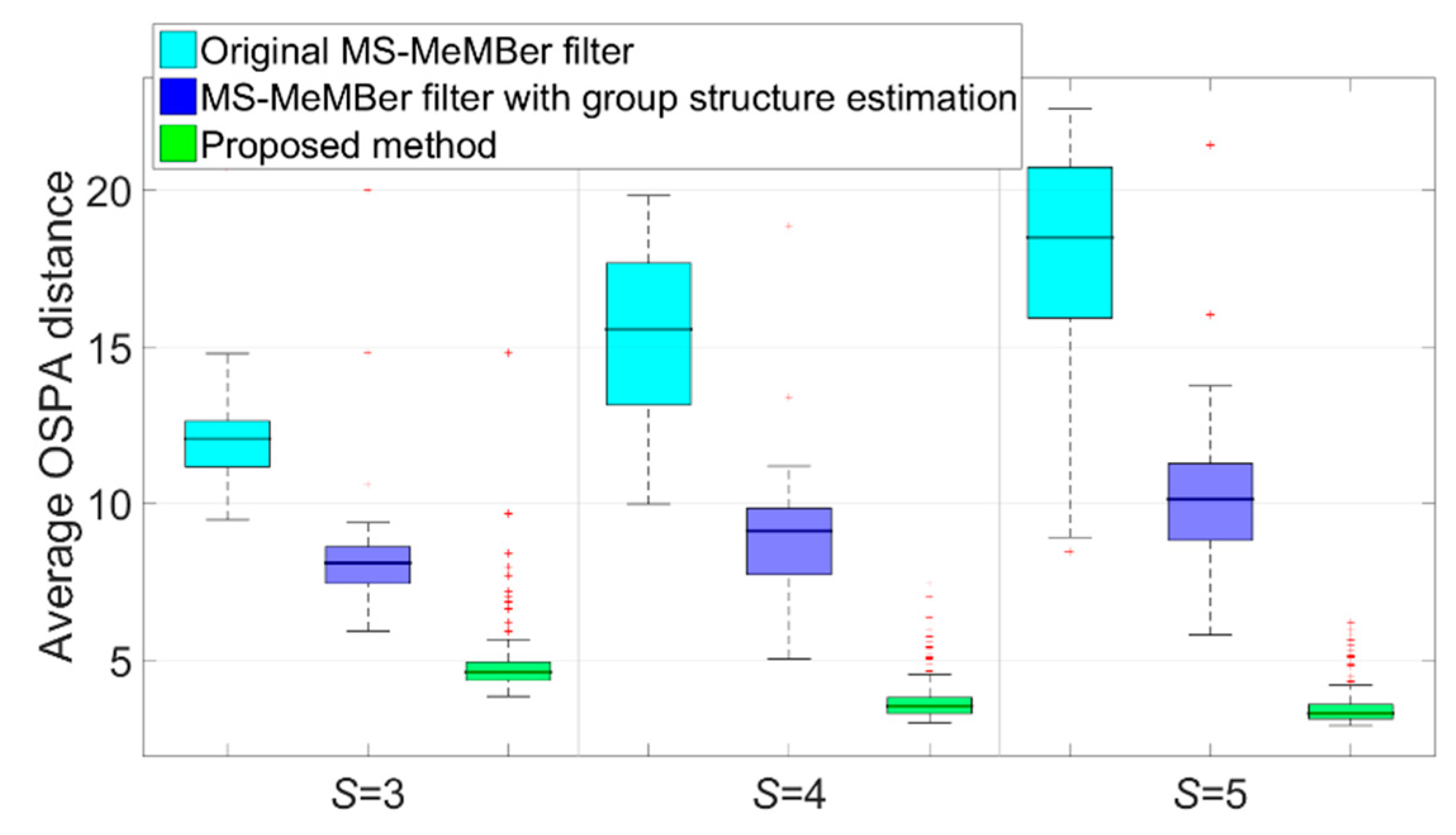
The time-averaged OSPA errors (via 50 MC runs) of the above methods in scenarios with different sensor numbers are displayed in Figure 11. It can be seen that as the number of the sensors increases, the time-average OSPA error of the two methods without MDA algorithm increases. The reason is that as S increases, the association between the measurements and Bernoulli components is more complicated because of the densely clustered members within the group. On the contrary, as the number of the sensors increases, the proposed method combined with the MDA algorithm and group structure estimation together can obtain better filtering results.

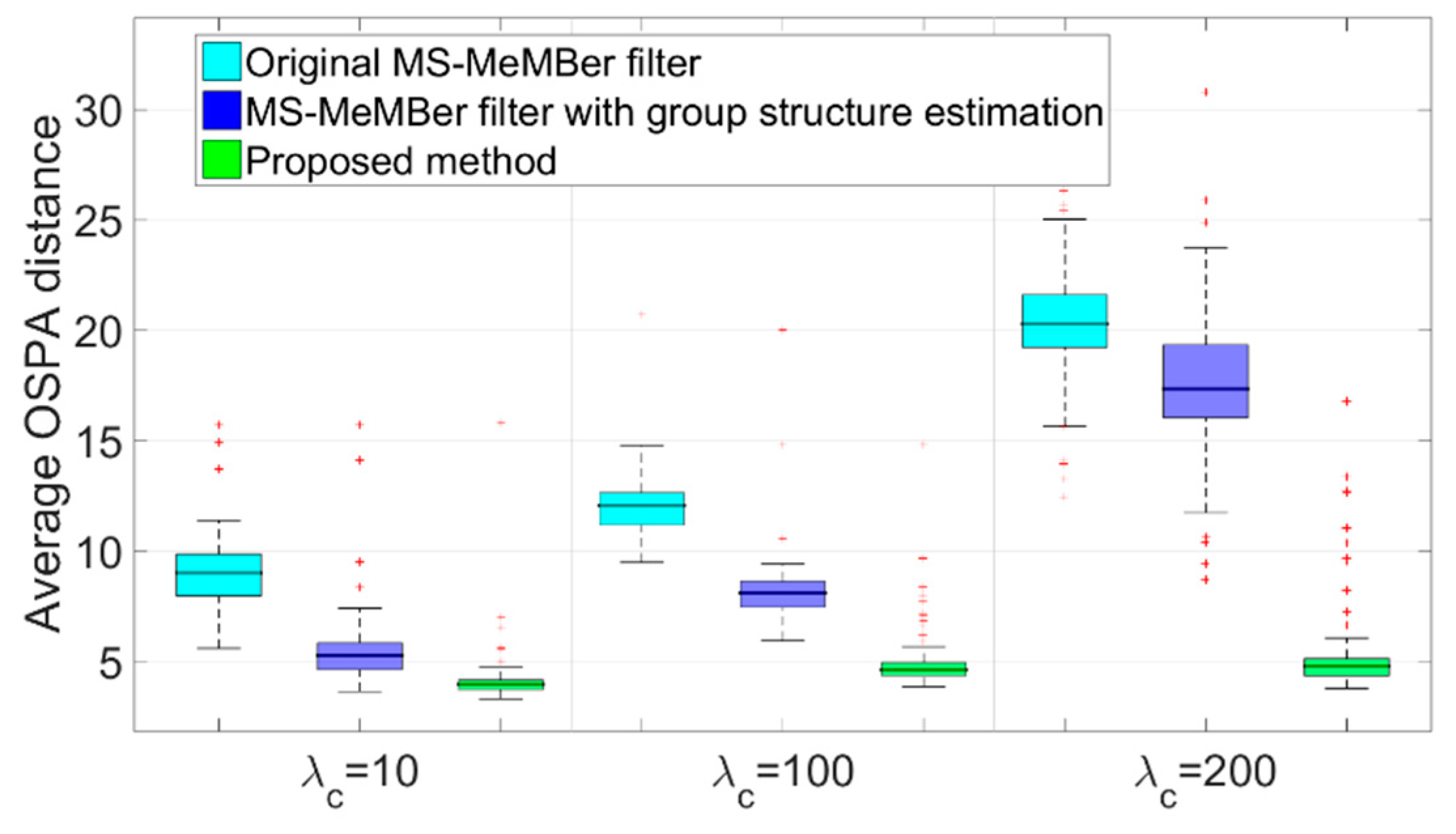
Figure 12 shows the performance of the original MS-MeMBer filter, the MS-MeMBer filter with group structure estimation, and the proposed method under different clutter intensities. The clutter intensity is varied in the range {10, 100, 200}. It can be concluded that the performance of the first two methods decreases significantly with the increase of clutter intensity. However, by using the MDA algorithm, the proposed method can still obtain better filtering results in clutter-intensive scenes.

5. Discussion

In this paper, we proposed a group target tracking method based on the MS-MeMBer filter. We used the group structure to constrain the movement of members within the group. We also improved the multi-sensor measurement partition through the MDA algorithm. Finally, we established a simulation scenario with splitting and merging of groups. Simulation results showed that compared with the original MS-MeMBer filter, the proposed method has achieved better robustness and accuracy in group target tracking scenarios, at the cost of an acceptable increasing computational load.

However, the MS-MeMBer filter is not strictly a tracker, because it can only get the target state, not the target trajectory. To obtain multi-target trajectories, the filter based on the labeled RFS or additional track maintenance operation can be considered. Furthermore, the proposed method ignores the dynamic evolution of the group structure. Future work will explore the multi-sensor multi-target filter, which can accommodate the evolution of group structures and can estimate target trajectories.