Moving to Automated Tree Inventory: Comparison of UAS-Derived Lidar and Photogrammetric Data with Manual Ground Estimates

Abstract

Unmanned aircraft systems (UAS) have advanced rapidly enabling low-cost capture of high-resolution images with cameras, from which three-dimensional photogrammetric point clouds can be derived. More recently UAS equipped with laser scanners, or lidar, have been employed to create similar 3D datasets. While airborne lidar (originally from conventional aircraft) has been used effectively in forest systems for many years, the ability to obtain important tree features such as height, diameter at breast height, and crown dimensions is now becoming feasible for individual trees at reasonable costs thanks to UAS lidar. Getting to individual tree resolution is crucial for detailed phenotyping and genetic analyses. This study evaluates the quality of three three-dimensional datasets from three sensors—two cameras of different quality and one lidar sensor—collected over a managed, closed-canopy pine stand with different planting densities. For reference, a ground-based timber cruise of the same pine stand is also collected. This study then conducted three straightforward experiments to determine the quality of the three sensors’ datasets for use in automated forest inventory: manual mensuration of the point clouds to (1) detect trees and (2) measure tree heights, and (3) automated individual tree detection. The results demonstrate that, while both photogrammetric and lidar data are well-suited for single-tree forest inventory, the photogrammetric data from the higher-quality camera is sufficient for individual tree detection and height determination, but that lidar data is best. The automated tree detection algorithm used in the study performed well with the lidar data, detecting 98% of the 2199 trees in the pine stand, but fell short of manual mensuration within the lidar point cloud, where 100% of the trees were detected. The manually-mensurated heights in the lidar dataset correlated with field measurements at r = 0.95 with a bias of −0.25 m, where the photogrammetric datasets were again less accurate and precise.

1. Introduction

Forest management often uses photogrammetry and more recently, lidar remote sensing as a tool to provide accurate information on the physical structure of forests [1,2,3,4]. An emerging platform for the remote sensing of forests is the unmanned aircraft system (UAS), a remotely-piloted or preprogrammed robotic aircraft equipped with a remote sensing payload [5,6,7]. UAS are quickly becoming the tool of choice for local-scale remote sensing projects due to their low entry cost and on-demand access to data collection, two traits that distinguish it from manned aircraft and satellite platforms. In parallel with the advent of accessible aerial platforms is the emergence of two remote sensing techniques for attaining three-dimensional (3D) information from UAS: structure-from-motion (SfM) photogrammetry and UAS laser scanning. SfM photogrammetry [8,9] enables production of dense, 3D reconstructions of the scene, using relatively inexpensive software to process photos taken with commercial, off-the-shelf (COTS) cameras [6]. The typically low flying heights of UAS missions allow for ground sample distances (GSDs) of the photos on the order of 1–3 cm, revealing the physical structure, or morphology, of the forest at a resolution that is unattainable from conventional remote sensing platforms. New lightweight laser scanners, such as the Velodyne VLP-16, also produce very high-resolution 3D point clouds on the order of 100–400 points/m², many orders of magnitude greater than conventional airborne laser scanning (ALS) [10,11]. These lightweight laser scanners, along with ever-lighter navigation sensors, stand to make UAS laser scanning more accessible and prevalent in the near future. The problem now facing the forest manager is analyzing these rich sources of 3D data.

Forest inventory and mensuration, considering the area and density of the typical forest, is an arduous task. The “standard” for forest mensuration, the timber cruise, requires selective sampling by a forester in the field to measure and estimate forest parameters such as tree count, diameter at breast height (DBH), tree height, stem form, and other physical traits [12]. It follows that the latest trend in forest inventory and mensuration is the use of automated systems, both for the collection and the processing of data [6,13,14,15,16,17]. Interest in the use of UAS has been growing in large part because they are more readily deployed and less cost prohibitive than manned aircraft. Among the more intriguing developments in forest inventory and mensuration is the automatic determination of forest parameters from lidar or photogrammetric point clouds [18,19,20,21]. Just as remarkable is the accuracy, repeatability, and efficiency with which these data can be collected [14,22]. The process by which individual tree parameters such as tree count, tree height, and crown area (to name a few) can potentially be identified is made possible not simply by advances in computing, but also by the increase in the density and quality of 3D structure of individual trees from low altitude [23,24,25].

In earlier photogrammetric approaches, a handful of crucial 3D points (e.g., the highest point of a crown) were manually located by a trained operator using a stereoscopic plotter, an instrument for manually recording the 3D positions of objects in overlapping (or stereo) images. Area-based image matching methods, such as those used in auto aerotriangulation (AT), could automatically generate match points between consecutive stereo images, but only under certain geometric and radiometric conditions (e.g., non-convergent photography, presence of contrast/texture). The dense, accurate 3D reconstruction of the forested area via SfM—referred to herein as a dense matching point cloud—is more efficient than auto AT in that it can produce feature matches in multiple, unordered images in various geometric configurations [8,26]. In a dense matching point cloud, that same tree is likely to have hundreds, possibly thousands, of 3D points associated with it; these results cannot be matched by conventional auto AT or a manual operator.

Early ALS data exhibited low return density, which led to underestimation of tree heights [27]. As lidar sensor technology advanced, the pulse rate and therefore return density attainable from lidar sensors increased such that sensing individual treetops became feasible. The amount of subcanopy information attainable via ALS also increased as lidar sensor technology advanced to multiple-return and full waveform systems. ALS data progressed from offering a low-density picture of the top of forest canopy and the ground below to many data points’ (i.e., laser pulse returns’) worth of information per tree, including information about the ground below the canopy. A more complete review of airborne laser scanning can be found in [28], and a further comparison between airborne photogrammetric and laser scanning can be found in [29].

The density of the data gleaned from both SfM and laser scanning allow for the detection of individual trees within the dataset. In many of the current methods of individual tree detection (ITD), the detection and segmentation of individual trees in a stand is accomplished by applying image processing methods to a rasterized canopy height model (CHM) such as watershed segmentation [30] or local maxima detection [31]. A host of other methods for detecting and delineating individual trees exist; a review of many of these methods can be found in the review by [32].

The accuracy of ITD depends on many factors related to the algorithms used; on a fundamental level, however, the quality of any ITD procedure is dependent upon the quality of the input data. The present work uses both photogrammetric and lidar data, the former of which is collected using two camera types commonly used for UAS photogrammetry, with the objective of identifying which datasets are of suitable quality for use in automated ITD. The data are subjected to both manual and automated ITD procedures, and the results are compared to those collected from an exhaustive timber cruise of 2199 trees in the study area. The automated ITD algorithm implemented uses no a priori information regarding the trees; location, spacing, and other tree parameters are not used as inputs. However, the experiment does test a matrix of parameters on each subplot of the study area with the objective of maximizing accuracy for each subplot for each dataset. This is done to give each dataset the best chance of success for each subplot conditions, thus providing a fair assessment of data quality among the datasets.

2. Materials and Methods

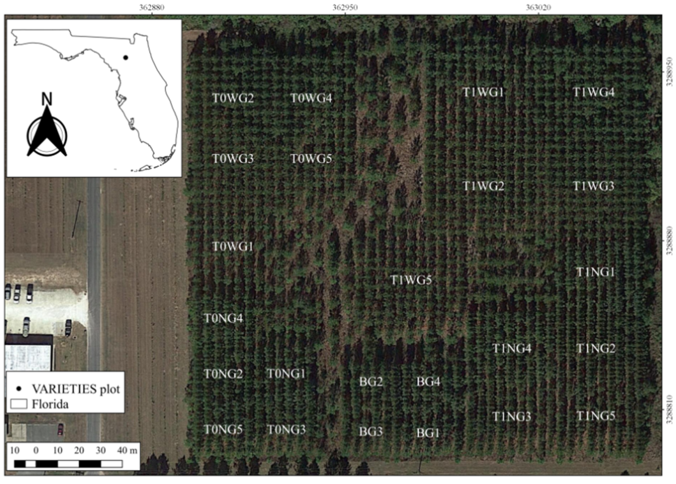
2.1. Study Area and Field Data Collection

This study was carried out on a single replicate of the VARIETIES II clonal test located in Gainesville, Florida, United States of America. The test contains five genetic entries of loblolly pine (Pinus taeda L.): three clones G1, G2, and G3; a full sib family, G4; and G5, a mixture of G1, G2 and G3 ramets. The clonal ramets were propagated via somatic embryogenesis. These genotypes and mixtures were planted under narrow (N)—1.83 m × 3.65 m, wide (W)—3.65 m × 3.65 m, and an independent Biomass (B)—3.65 m × 1.83 m spacings. The trial is designed such that some plots will be thinned (T1) and others not thinned (T0) (Figure 1), but at the time of the study, this planned thinning had not taken place.

The seedlings were planted in February 2010 with beds running north to south (Figure 1). The plots in wide spacing and no thinning (T0W) were formed with 8 rows × 9 trees; trees under wide spacing under thinning (T1W) contained 11 rows × 11 trees. Tree plots in narrow spacing and no thinning (T0N) were designed with 6 rows × 12 trees, and the tree plots under narrow spacing and thinning (T1N) were formed by 9 rows × 16 trees. Tree plots in biomass spacing (B) were formed with 6 rows × 10 trees.

The timber cruise was performed in mid-March 2018 in the previously established plots. In each plot, measures included diameter at breast height (DBH) and stem counts for all trees, and total tree height on a sample of appropriate trees per plot. In all, DBH was measured on 2199 trees and tree height on 450 trees.

2.2. Unnamed Aircraft Systems Surveying

This study used two UAS platforms and three different sensors. The first aerial survey was conducted on 2 March 2018 using a DJI Phantom 4 Pro UAS equipped with the DJI FC6310 RGB wide-angle digital camera. The DJI wide-angle camera triggered 220 times during the flight, capturing an area of approximately 21 ha with 12.4-megapixel resolution and an 84° field of view. With a focal length of 8.8 mm (20 mm, 35 mm equivalent) and pixel size 2.41 µm while flying at 122 m height above ground the camera yielded a ground sample distance (GSD) of approximately 3.1 cm. (A greater area was covered by this survey to accommodate another simultaneous study.)

The second aerial survey occurred on 14 March 2018 using the DJI-S1000+ platform equipped with the Canon EOS REBEL SL1, a digital single-lens reflex (DSLR) camera. From a 100 m height above ground, an area of approximately 7.8 ha was captured using a total of 369 images at 17.9-megapixel resolution with a 59° field of view, focal length 24 mm, and pixel size 4.38 µm, yielding a GSD of approximately 1.6 cm.

Table 1. Summary of wide-angle and DSLR image processing in Agisoft PhotoScan Professional.

Attribute	Wide-Angle	DSLR
Number of images	220	369
Flying altitude (m)	122	100
Nominal front/side overlap	90%/75%	90%/70%
GSD (cm/pix)	3.1	1.6
Coverage area (ha)	21	7.8
Tie points	202,622	14,314
Projections	742,332	53,713
Reprojection error (pix)	0.465	0.364
Key point/tie point limit	60,000/0
Dense point cloud quality	medium
Depth filtering	disabled

summarizes statistics for both flights and their processing. (Though both cameras technically have a wide-angle lens, for the purposes of distinguishing the two in the text, the former is referred to as wide-angle, and the latter as DSLR.)

UAS lidar data were also acquired on 14 March 2018 using the Velodyne VLP-16 laser scanner mounted aboard the DJI-S1000+, and navigation data were collected with an onboard Novatel SPAN-IGM-S1, a combined global navigation satellite system (GNSS) receiver and inertial navigation system (INS). The flying height was 30 m. The nominal footprint of the laser beam was 9 cm, and the resulting point cloud had a mean sampling density of 150 points/m².

2.3. Point Cloud Processing

For both DSLR and wide-angle image processing, a total of 369 and 220 images, respectively, from the flights conducted over the study area were used to generate point clouds using the Agisoft PhotoScan Professional v. 1.4.2 software (now called Agisoft Metashape) [33]. For both UAS imagery surveys, direct georeferencing (or airborne control) was used to georeference the data collected. In other words, a GNSS sensor onboard each UAS recorded the position of the aircraft each time a photo was captured. The processing steps for both the wide-angle and DSLR images included automatic aerial triangulation, bundle block adjustment, noise filtering and point cloud classification. The workflow presented by the USGS National UAS Project Office [34] was used to ensure the highest-quality feature matches among the sets of photos were used to generate the resulting dense-matching point cloud, which prevents artifacts in the point cloud generation such as “doming”, or warping of the study area being reconstructed. One notable departure from the USGS workflow is that the depth filtering setting in Photoscan was disabled. While this necessarily results in a noisier point cloud, noise filtering was undertaken in a subsequent step.

The navigation data from the lidar survey were filtered using NovAtel Inertial Explorer software [35]. The filtered navigation data and raw lidar data were then processed in custom software written in the Python programming language to create a georeferenced point cloud. The lidar point cloud was then filtered in CloudCompare v. 2.8 open-source software [36] using the Statistical Outlier Removal (SOR) tool with six-point mean distance estimation, and a one standard deviation multiplier threshold [32]. Afterwards, the point cloud was normalized in LAStools [37], classifying the ground via LASground and calculating the height above ground of all points by LASheight, resulting in a normalized point cloud.

Subsequently, the wide-angle and DSLR point clouds were filtered and normalized in the same manner as the lidar data. Then the normalized point clouds were rasterized in CloudCompare to obtain a canopy height model (CHM) for each dataset, using the cell maximum height. The CHM raster cell size (i.e., pixel size) was set to 16.7 cm (36 pixels/m²), with empty cells filled with minimum height. The CHMs were used as input in the automated individual tree detection detailed in Section 2.4.

Figure 2. Data processing workflow showing the steps taken from point cloud processing, canopy height model (CHM) generation, smoothing window sizes (SWS), search window sizes (FWS), to individual tree detection (ITD) and tree height measurement and validation against the timber cruise. This flow chart includes the workflows for both the manual and automated tree mensuration detailed in this study. (This workflow excludes the steps taken to generate the point clouds, which are detailed in Section 2.3.)

2.4. Individual Tree Detection and Tree Height Measurement

After the point cloud processing for the three datasets, the trees were manually and visually identified in each point cloud, and the tree heights were measured using the point picking tool in CloudCompare. The tree height was taken by the highest point of each tree manually identified. The mensuration of the trees in the point clouds were performed by the same user with a priori knowledge of the study site, but without knowledge of the results of the timber cruise detailed in Section 2.1.

Using the rLiDAR package [38] for the R programming language [39], the CHM was processed by a mean smooth filter testing with five smoothing window sizes (SWS) of 3 × 3, 5 × 5, 7 × 7, 9 × 9, and 11 × 11 pixels. In the rLiDAR package the FindTreesCHM function was used to automate ITD. This function offers an option to search for treetops in the CHM via moving window with a Fixed Window Size (FWS). Similar to the SWS test, we tested five search window sizes (FWS) of 3 × 3, 5 × 5, 7 × 7, 9 × 9, and 11 × 11 pixels. The automated ITD was performed using a 2-m height threshold (i.e., any detected tree less than 2 m height was omitted). Figure 2 summarizes the workflow of the study methodology.

2.5. Statistical Analysis

The accuracies of both the manual and automatic ITD were evaluated in terms of true positive (TP, correct detection), false negative (FN, omission error) and false positive (FP, commission error). The recall (r_e, tree detection rate), precision (p, correctness of the detected trees) and F-score (F, overall accuracy) were then calculated as follows [31,40]:

$$r_e=\raisebox{1ex}{$\mathrm{TP}$}\!\left/ \!\raisebox{-1ex}{$\left(\mathrm{TP}+\mathrm{FN}\right)$}\right.$$

(1)

$$p=\raisebox{1ex}{$\mathrm{TP}$}\!\left/ \!\raisebox{-1ex}{$\left(\mathrm{TP}+\mathrm{FP}\right)$}\right.$$

(2)

$$F=2\times \left(\raisebox{1ex}{$r_e\times p$}\!\left/ \!\raisebox{-1ex}{$\left(r_e+p\right)$}\right.\right)$$

(3)

As previously mentioned, this experiment tests a matrix of parameters in the automated ITD algorithm used with the objective of maximizing accuracy for each subplot for each dataset. This is done to give each dataset the best chance of success for each subplot’s conditions. More specifically, for each of the three datasets, each subplot (T0NG1, T0NG2, etc.) was subjected to automated ITD under the 25 combinations of SWS and FWS stated in Section 2.4. For each subplot in each dataset, the best combination of SWS and FWS was determined by which yielded the highest F-score.

To further analyze under which conditions each dataset correctly or incorrectly identified trees, kernel density plots for TP, FN, and FP were created for each sensor with tree DBH as the abscissa. The bandwidth for the kernel density plots was chosen according to Silverman’s rule of thumb [41].

3. Results

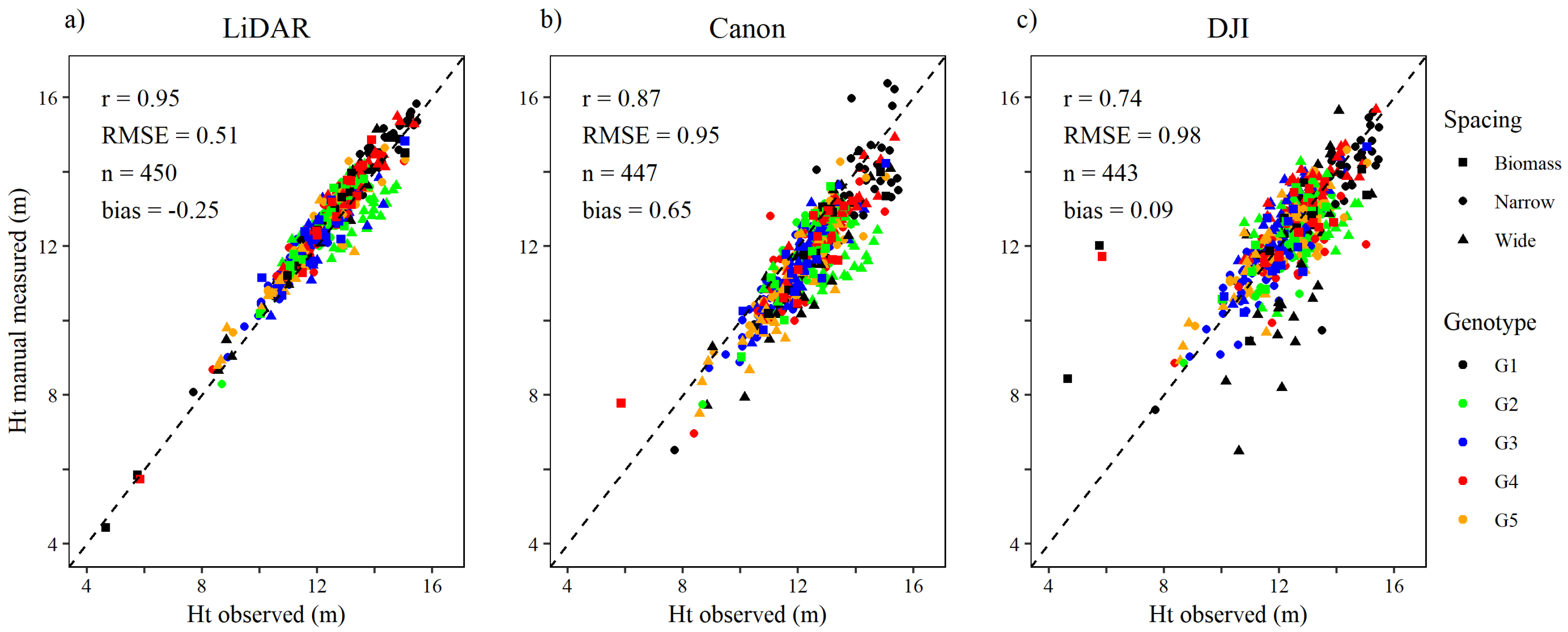
3.1. Manual Individual Tree Detection and Tree Height Measurement

All trees from the timber cruise were manually identified in the lidar point cloud. In contrast to lidar, in the DSLR dense matching point cloud manual tree detection resulted in 14 missed trees (0.63%), or false negatives, and the wide-angle point cloud yielded 30 missed trees (1.36%) (

Table 2. Accuracy assessment results of DSLR- and wide-angle-derived manual individual tree detection based on false positive (FP), false negative (FN), true positive (TP), recall (r_e), precision (p) and F-score (F) statistics. Note: The results for manual tree detection in the lidar point cloud are omitted from this table because the true positive detection rate was exactly 100%.

T	S	G	n	-------------------------------- DSLR ------------------------------						------------------------------ Wide-Angle ------------------------------
				FP	FN	TP	re	p	F	FP	FN	TP	re	p	F
-	B	G1	57	0	2	55	0.96	1	0.98	0	0	57	1	1	1
-	B	G2	58	0	0	58	1	1	1	0	0	58	1	1	1
-	B	G3	59	0	0	59	1	1	1	0	0	59	1	1	1
-	B	G4	59	0	1	58	0.98	1	0.99	0	0	59	1	1	1
0	N	G1	60	0	0	60	1	1	1	0	0	60	1	1	1
0	N	G2	65	0	0	65	1	1	1	0	0	65	1	1	1
0	N	G3	71	0	0	71	1	1	1	0	0	71	1	1	1
0	N	G4	69	0	0	69	1	1	1	0	0	69	1	1	1
0	N	G5	71	0	0	71	1	1	1	0	0	71	1	1	1
1	N	G1	140	0	1	139	0.99	1	1	0	1	139	0.99	1	1
1	N	G2	143	0	0	143	1	1	1	0	0	143	1	1	1
1	N	G3	141	0	0	141	1	1	1	0	0	141	1	1	1
1	N	G4	140	0	0	140	1	1	1	0	0	140	1	1	1
1	N	G5	140	0	2	138	0.99	1	0.99	0	0	140	1	1	1
0	W	G1	63	0	2	61	0.97	1	0.98	0	8	55	0.87	1	0.93
0	W	G2	71	0	0	71	1	1	1	0	0	71	1	1	1
0	W	G3	72	0	0	72	1	1	1	0	0	72	1	1	1
0	W	G4	69	0	0	69	1	1	1	0	0	69	1	1	1
0	W	G5	65	0	2	63	0.97	1	0.98	0	7	58	0.89	1	0.94
1	W	G1	109	0	1	108	0.99	1	1	0	6	103	0.94	1	0.97
1	W	G2	120	0	0	120	1	1	1	0	0	120	1	1	1
1	W	G3	121	0	0	121	1	1	1	0	0	121	1	1	1
1	W	G4	117	0	0	117	1	1	1	0	0	117	1	1	1
1	W	G5	119	0	3	116	0.97	1	0.99	0	8	111	0.93	1	0.97
Total			2199	0	14	2185	0.99	1	1	0	30	2169	0.98	1	0.99

T: Thinning; S: Spacing; G: Genotype; n: Number of trees.

). Unexpectedly, in the wide-angle camera’s point cloud, 29 of the 30 missed trees were in wide spacing plots.

Relative to manual measurements of tree height, the height measurements taken from the lidar point cloud were more precise than both RGB sensors (Figure 3). The relationship between tree height observed in ground-based inventory measurements and tree height from the lidar point cloud was strong (r = 0.95), the root mean square error (RMSE) was approximately 0.5 m, and the tree height measured were overestimated slightly (bias = −0.25 m). With the DSLR dense matching point cloud tree heights were underestimated (bias = 0.65 m), with strong relationship between observed and measured tree height (r = 0.87) and RMSE of 0.95 m. With the wide-angle dense matching point cloud, measured tree height correlated weakest (r = 0.74), with RMSE of 0.98 m, but the bias was close to zero.

Figure 4 shows the canopy height models (CHMs) generated from sensor point clouds. The description of the canopy from the three sensors agreed well overall, but the heights from the DSLR and wide-angle dense matching clouds were often below those obtained with lidar (Figure 4e,f). Similarly, the heights of trees from the DSLR dense matching cloud were often greater than those from the wide-angle dense matching cloud. In contrast, heights in T0N and B (southwest plots) from the wide-angle dataset were often above those of the DSLR dataset (Figure 4b,c,f).

Compared with the DSLR- and wide-angle-derived CHMs, the lidar CHM showed an increased level of detail, with smaller gaps in the canopy (Figure 4a–c). Changes in stand density were also better characterized in the lidar CHM. Mainly in trees under wide spacing, the gaps were greater, and some trees were lost in DSLR- and especially wide-angle-RGB CHMs.

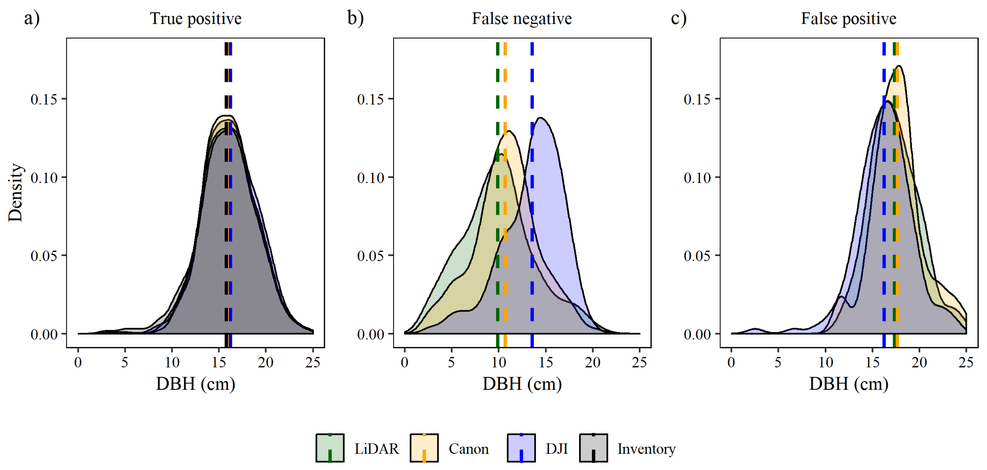
3.2. Automated Individual Tree Detection from Canopy Height Models

The automated FindTreesCHM algorithm proved effective but variable for detecting individual trees. Choosing the best combination of smoothing window sizes (SWS) and search window sizes (FWS) affected the accuracy of automated ITD for all sensors. While 25 combinations of SWS and FWS were tested for each of the three sensors as detailed in Methods, only the SWS/FWS combination with the highest overall accuracy, or F-score (Equation (3)), was used for each plot type. The accuracy of automated ITD for biomass (B) and narrow spacing (N) were highest using 5 × 5 SWS and 7 × 7 FWS (excepting the DSLR sensor and its 3 × 3 SWS). On the other hand, the plots with wide spacing (W) had higher F-scores with the larger 9 × 9 SWS and FWS (7 × 7 and 7 × 7 for the DSLR).

For the lidar CHM, the recall (r_e) had an overall value of 0.96 with range of 0.82 to 1.00; overall value of precision (p) was 0.99 with a range of 0.96 to 1.00; and the average F-score was 0.98 with a range of 0.90 to 1.00. In short, 2120 of trees (96%) were correctly detected, or true positives; 23 trees were false positives (FP); and the algorithm missed 79 trees identified in the timber cruise, or false negatives. For the DSLR CHM, the overall recall was 0.93 with range of 0.78 to 1.00; overall p-value was 0.97 with a range of 0.88 to 1.00; and the average F-score was 0.95 with a range of 0.87 to 1.00. In this CHM, the algorithm classified 2029 trees (92%) as true positives, 57 trees as false positives, and 170 trees were missed. For the wide-angle CHM, recall had an overall value of 0.83 with a range of 0.33 to 1.00; overall p-value of 0.92 with a range of 0.78 to 1.00; and the average F-score was 0.86 with a range of 0.50 to 0.96. In this CHM, the algorithm correctly classified 1824 trees (83%) as true positives, 169 trees as false positives, and 375 trees were missed. A detailed summary of these findings is presented in

Table 3. Accuracy assessment results of lidar, DSLR and wide-angle automated individual tree detection based on false positive (FP), false negative (FN), true positive (TP), recall (r_e), precision (p) and F-score (F) statistics.

T	S	G	n	----------------------- Lidar ---------------------								-------------------- DSLR Camera -----------------								---------------- Wide-Angle Camera --------------
				SWS	FWS	FP	FN	TP	re	p	F	SWS	FWS	FP	FN	TP	re	p	F	SWS	FWS	FP	FN	TP	re	p	F
-	B	G1	57	5 × 5	7 × 7	1	10	47	0.82	0.98	0.90	3 × 3	7 × 7	1	11	46	0.81	0.98	0.88	5 × 5	7 × 7	4	7	50	0.88	0.93	0.90
-	B	G2	58	5 × 5	7 × 7	0	0	58	1.00	1.00	1.00	3 × 3	7 × 7	1	2	56	0.97	0.98	0.97	5 × 5	7 × 7	6	4	54	0.93	0.90	0.92
-	B	G3	59	5 × 5	7 × 7	2	5	54	0.92	0.96	0.94	3 × 3	7 × 7	3	7	52	0.88	0.95	0.91	5 × 5	7 × 7	7	10	49	0.83	0.88	0.85
-	B	G4	59	5 × 5	7 × 7	0	2	57	0.97	1.00	0.98	3 × 3	7 × 7	4	3	56	0.95	0.93	0.94	5 × 5	7 × 7	12	9	50	0.85	0.81	0.83
0	N	G1	60	5 × 5	7 × 7	0	0	60	1.00	1.00	1.00	3 × 3	7 × 7	0	2	58	0.97	1.00	0.98	5 × 5	7 × 7	5	7	53	0.88	0.91	0.90
0	N	G2	65	5 × 5	7 × 7	0	2	63	0.97	1.00	0.98	3 × 3	7 × 7	0	5	60	0.92	1.00	0.96	5 × 5	7 × 7	7	4	61	0.94	0.90	0.92
0	N	G3	71	5 × 5	7 × 7	3	4	67	0.94	0.96	0.95	3 × 3	7 × 7	6	5	66	0.93	0.92	0.92	5 × 5	7 × 7	7	12	59	0.83	0.89	0.86
0	N	G4	69	5 × 5	7 × 7	1	3	66	0.96	0.99	0.97	3 × 3	7 × 7	3	4	65	0.94	0.96	0.95	5 × 5	7 × 7	17	9	60	0.87	0.78	0.82
0	N	G5	71	5 × 5	7 × 7	1	4	67	0.94	0.99	0.96	3 × 3	7 × 7	3	2	69	0.97	0.96	0.97	5 × 5	7 × 7	14	5	66	0.93	0.83	0.87
1	N	G1	140	5 × 5	7 × 7	7	10	130	0.93	0.95	0.94	3 × 3	7 × 7	3	31	109	0.78	0.97	0.87	5 × 5	7 × 7	6	29	111	0.79	0.95	0.86
1	N	G2	143	5 × 5	7 × 7	2	2	141	0.99	0.99	0.99	3 × 3	7 × 7	3	11	132	0.92	0.98	0.95	5 × 5	7 × 7	8	16	127	0.89	0.94	0.91
1	N	G3	141	5 × 5	7 × 7	1	7	134	0.95	0.99	0.97	3 × 3	7 × 7	6	26	115	0.82	0.95	0.88	5 × 5	7 × 7	8	43	98	0.70	0.92	0.79
1	N	G4	140	5 × 5	7 × 7	2	8	132	0.94	0.99	0.96	3 × 3	7 × 7	5	10	130	0.93	0.96	0.95	5 × 5	7 × 7	14	16	124	0.89	0.90	0.89
1	N	G5	140	5 × 5	7 × 7	1	10	130	0.93	0.99	0.96	3 × 3	7 × 7	0	25	115	0.82	1.00	0.90	5 × 5	7 × 7	16	24	116	0.83	0.88	0.85
0	W	G1	63	9 × 9	9 × 9	0	3	60	0.95	1.00	0.98	7 × 7	7 × 7	0	3	60	0.95	1.00	0.98	9 × 9	9 × 9	0	42	21	0.33	1.00	0.50
0	W	G2	71	9 × 9	9 × 9	0	0	71	1.00	1.00	1.00	7 × 7	7 × 7	2	0	71	1.00	0.97	0.99	9 × 9	9 × 9	6	0	71	1.00	0.92	0.96
0	W	G3	72	9 × 9	9 × 9	1	0	72	1.00	0.99	0.99	7 × 7	7 × 7	10	0	72	1.00	0.88	0.94	9 × 9	9 × 9	5	6	66	0.92	0.93	0.92
0	W	G4	69	9 × 9	9 × 9	0	1	68	0.99	1.00	0.99	7 × 7	7 × 7	2	1	68	0.99	0.97	0.98	9 × 9	9 × 9	5	2	67	0.97	0.93	0.95
0	W	G5	65	9 × 9	9 × 9	0	3	62	0.95	1.00	0.98	7 × 7	7 × 7	1	5	60	0.92	0.98	0.95	9 × 9	9 × 9	0	21	44	0.68	1.00	0.81
1	W	G1	109	9 × 9	9 × 9	0	1	108	0.99	1.00	1.00	7 × 7	7 × 7	0	5	104	0.95	1.00	0.98	9 × 9	9 × 9	1	27	82	0.75	0.99	0.85
1	W	G2	120	9 × 9	9 × 9	0	0	120	1.00	1.00	1.00	7 × 7	7 × 7	0	1	119	0.99	1.00	1.00	9 × 9	9 × 9	4	19	101	0.84	0.96	0.90
1	W	G3	121	9 × 9	9 × 9	0	0	121	1.00	1.00	1.00	7 × 7	7 × 7	1	0	121	1.00	0.99	1.00	9 × 9	9 × 9	8	5	116	0.96	0.94	0.95
1	W	G4	117	9 × 9	9 × 9	1	2	115	0.98	0.99	0.99	7 × 7	7 × 7	3	3	114	0.97	0.97	0.97	9 × 9	9 × 9	8	3	114	0.97	0.93	0.95
1	W	G5	119	9 × 9	9 × 9	0	2	117	0.98	1.00	0.99	7 × 7	7 × 7	0	8	111	0.93	1.00	0.97	9 × 9	9 × 9	1	55	64	0.54	0.98	0.70
Total			2199	-	-	23	79	2120	0.96	0.99	0.98	-	-	57	170	2029	0.93	0.97	0.95	-	-	169	375	1824	0.83	0.92	0.86

T: Thinning; S: Spacing; G: Genotype; n: Number of trees; SWS: Smoothing Window Size; FWS: Fixed Window Size.

.

For all sensor CHMs, more trees were classified as false negatives than false positives, i.e., under detection was greater than over detection. On average, the FindTreesCHM algorithm worked best with the lidar CHM, which was more accurate than the DSLR CHM, which was more accurate than the wide-angle CHM.

In the manual ground-based inventory data, trees with a fork below DBH are considered two individuals and two tree heights can be computed. When the stem fork starts above DBH the tree is considered a unique individual and the tallest stem is computed. In this study, some trees were classified as forked. In addition, some trees where the algorithm found more than one top (a false positive) these trees were evaluated to check if they were forked. No trees classified as false positive in the lidar CHM were forked (

Table 4. Forked trees classified as false positive (FP) in different sensors.

					Forked Trees Classified as FP
T	S	G	n	Forked Trees	Lidar	DSLR	Wide-Angle
-	B	G1	57	3	0	0	0
-	B	G2	58	3	0	0	1
-	B	G3	59	8	0	0	0
-	B	G4	59	5	0	1	0
0	N	G1	60	2	0	0	0
0	N	G2	65	6	0	0	1
0	N	G3	71	11	0	1	0
0	N	G4	69	2	0	0	0
0	N	G5	71	4	0	0	0
1	N	G1	140	15	0	0	1
1	N	G2	143	12	0	1	0
1	N	G3	141	16	0	0	0
1	N	G4	140	13	0	1	1
1	N	G5	140	8	0	0	1
0	W	G1	63	1	0	0	0
0	W	G2	71	12	0	0	0
0	W	G3	72	5	0	0	1
0	W	G4	69	8	0	0	3
0	W	G5	65	7	0	1	0
1	W	G1	109	10	0	0	0
1	W	G2	120	8	0	0	0
1	W	G3	121	16	0	0	2
1	W	G4	117	14	0	0	0
1	W	G5	119	4	0	0	0
Total			2199	193	0	5	11

T: Thinning; S: Spacing; G: Genotype; n: Number of trees.

). Nevertheless, 5 (8.8%) and 11 (6.5%) trees classified as false positive respectively in the DSLR and wide-angle CHMs were forked. However, the percentage of forked trees was small, hence the false positive problem is probably related to other variables affecting CHM quality.

Analyzing true positive trees by DBH kernel and average, the density distributions for each sensor shows that all sensors were well correlated with the timber cruise (Figure 5a). DBH averaged 15.77 cm in the inventory 16.05 cm for the lidar CHM, 16.15 for DSLR CHM, and 16.22 cm for the wide-angle CHM. In trees classified as FN, the lidar CHM average and distribution shifted to smaller DBHs (9.89 cm), the DSLR CHM average and distribution shifted to DBHs (10.71 cm) closer to lidar CHM; and the wide-angle CHM average and distribution were shifted to larger DBH (13.56 cm) (Figure 5b). In trees classified as FP, the DSLR CHM average and distribution shifted to higher DBHs (17.63 cm) (Figure 5c). The lidar CHM average and distribution shifted to DBH 17.33 cm; and the wide-angle CHM average and distribution shifted to DBH as 16.25 cm.

In contrast, the distribution shifted to smaller DBH in trees classified as FP, lidar and DSLR distributions shifted to trees with higher DBH (Figure 5c). On average, within the wide-angle data trees with lower DBH (16.24 cm) were classified as FP, followed by the lidar CHM with 17.33 cm and DSLR CHM with 17.63 cm.

4. Discussion

The VARIETIES II trial was chosen as an “ideal” case to evaluate UAS phenotyping, because the site is flat, clean of understory and contained blocks of a full sib family and three clones and mixtures of these clones planted at three spacings, and manual ground-based measurements of tree inventory, DBH and height were available from winter of 2018 for comparison. UAS showed promise for tree inventory and improving height measurements in young pine research trials. The positions of all trees were known from planting and previous inventories, which facilitated their manual identification in the CHM. With the lidar all trees were identified and manual estimation of tree height using available tools resulted in a very strong correlation (r = 0.95) between ground and lidar heights.

The DSLR performed better than the wide-angle camera with manual tree identification. The DSLR dataset yielded half the number of false negative trees, although FN from both sensors were very low, and a stronger correlation (r = 0.87 vs. r = 0.74) with manual ground-based height measurements from the timber cruise. The RMSE in height measurement was the lowest from lidar and similar for the DSLR and wide-angle datasets. Overall, the best results with manual tree identification were obtained with lidar (Figure 3).

While manual tree identification and height estimation in the small dataset here was not time intensive, we investigated available approaches to automate the tree identification and tree height estimation for larger datasets. We evaluated the method of [31] as available in the rLiDAR package with CHMs derived from a low-altitude lidar point cloud, as well as dense matching point clouds derived from both DSLR (longer focal length) and wide-angle (shorter focal length) digital cameras. Using data smoothing windows optimized for spacing, the results show that the lidar data gave half the number of false negative and false positive trees identified within the DSLR dataset and one quarter identified within the wide-angle dataset (Table 3).

It is known that forest types, tree heights, tree ages and canopy closures may affect the SWS and FWS combinations and the local maximum tree identification model [42,43,44]. In our study, better results were found using the smaller window SWS and FWS combinations for narrow spacing than with trees in wide spacing, possibly because of the direct relationship between canopy closure and tree spacing. As tree spacing is important to the smoothing and search algorithm, the accuracy in identifying trees with this algorithm may be decreased under mixed spacing and/or in natural stands [31]. Guerra-Hernandez et al. [45], using a different combination of SWS and FWS and implementing the algorithm proposed by [46] on both airborne laser scanning (ALS) and SfM data for a Eucalyptus stand under 3.70 × 2.50 m tree spacing, found results similar to those of the lidar CHM automated process here with pine. However, both the SWS and FWS were smaller with Eucalyptus than those found to be optimal in our study, even though the tree spacing was greater. Beyond the difference between species in both studies, the algorithm choice is another factor that may influence SWS and FWS optimization.

Moreover, it was verified that tree forking did not contribute significantly to the false positives with any sensor (Table 4). This is important because some of pine species and families have a high rate of forking and the algorithm is able to detect the individuals that are unforked. Analysis of the false negatives with stem diameter from the ground-based inventory showed that only smaller-diameter trees were more often not detected with lidar and the DSLR sensors. In contrast, the wide-angle sensor missed more larger-diameter trees and the mean of false negative stem diameter from the ground-based inventory was greater than with the lidar and DSLR sensors. Analysis of the false positives with ground-based stem diameters showed that larger diameter trees were more often detected correctly with lidar and the DSLR sensors and just the biggest trees were wrongly classified as two or more individuals (false positives). The wide-angle sensor detected trees with larger stem diameter without problems and explains why the false positive with this sensor was lower than the other sensors.

4.1. Quality Assurance of Dense-Matching Point Clouds from Imagery

The guidance offered in [34] for generating a dense matching point cloud from UAS imagery is a helpful, but not definitive, guide. Efforts must be taken to ensure the quality of the images and of the subsequent data products, such as the bare-earth digital elevation model (DEM) and canopy height model (CHM). Care must also be taken to select the correct parameters in Agisoft Metashape or comparable software to create the highest-quality product. Exhaustive testing of different combinations of these parameters warrants its own case study but falls outside of the scope of the study presented here. For fairness of comparison, both imagery datasets were processed similarly (see Table 1 and Section 2.3).

Shadows in imagery can create artifacts in the resulting point cloud such as noise or missing information. For the even-aged pine stand used in this study, the effects of shadows were minimal; the trees are all about the same height and do not cast shadows onto the tree crowns to the north of them in our imagery, taken in March in Florida. Both imagery flights were conducted about the same time of day and less than two weeks apart, so sun angle differences are negligible. These conditions are nearly ideal and should not be considered typical. (The more ideal setting would have been to capture the imagery on cloudy days in order to take advantage of the diffuse light and minimal shadows.)

DEM comparison among the three sensors’ datasets revealed no notable differences, and therefore they are not presented as results of this study. This also should not be considered a typical result, however. The site used for this study is a former agricultural area, and the ground is very flat with practically no slope, and the canopy is sufficiently open to allow image matching to occur along the ground beneath the canopy. The quality of DEM between imagery and lidar may vary greatly depending on canopy conditions. For example, when capturing imagery of a tightly closed canopy, a camera may not be able to capture many images that include the ground, and the resulting DEM would be subject to errors. Lidar, an active sensor which emits and detects its own energy, has the advantage of needing less canopy opening to detect the ground beneath.

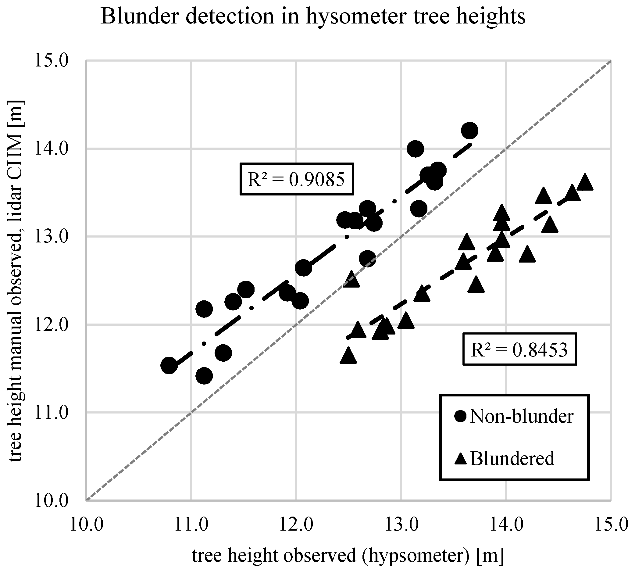
4.2. Detecting Errors in the Timber Cruise

Clone G2 in wide spacing (WG2) was consistently underestimated with manual ground measurements compared with lidar, which likely contributed to the slight negative bias of the estimate. The authors hypothesize that the manual ground-based measurement may be incorrect, because the lidar ground model used for estimating heights was well supported across the site. While analyzing the tree height observations, a likely blunder was detected in the timber cruise data. For 20 stems measured consecutively, an average overestimation of 0.90 m was present. The expected bias between the hypsometer-measured heights in the timber cruise and the lidar-derived heights is negative, i.e., the hypsometer is expected to underestimate the heights of the trees due to the pose of the hypsometer. The lidar-derived heights of the trees are expected to be closer to the true value. Thus, an average overestimation by the hypsometer of 0.90 m, when on average the hypsometer underestimated heights by 0.25 m (Figure 6), stood out as a blunder.

5. Conclusions

This study investigated the quality of both photogrammetric and lidar 3D datasets collected from UAS remote sensing platforms. Each of the datasets were subjected to manual tree detection and manual height estimation as well as automated individual tree detection using the rLiDAR software package. The results of each of the three experiments on the three datasets were compared to timber cruise data. The objective of examining the datasets comparatively was to identify which were suitable for use for automated individual tree detection. The wide-angle DJI camera performed reasonably well (F-score of overall accuracy 0.86), while the DSLR camera and lidar sensors performed exceptionally (F-scores 0.95 and 0.98, respectively). Overall, the best data were obtained with lidar and the poorest with the shorter-focal-length, wide-angle lens camera. The lidar and DSLR datasets’ height estimates compared very well with ground-based methods.

References

1. Lim, K.; Treitz, P.; Wulder, M.; St-Onge, B.; Flood, M. LiDAR Remote Sensing of Forest Structure. Prog. Phys. Geogr. Earth Environ. 2003, 27, 88–106. [Google Scholar] [CrossRef] [Green Version]
2. Lefsky, M.A.; Cohen, W.B.; Parker, G.G.; Harding, D.J. Lidar Remote Sensing for Ecosystem Studies. BioScience 2002, 52, 19–30. [Google Scholar] [CrossRef]
3. Miller, D.R.; Quine, C.P.; Hadley, W. An Investigation of the Potential of Digital Photogrammetry to Provide Measurements of Forest Characteristics and Abiotic Damage. For. Ecol. Manag. 2000, 135, 279–288. [Google Scholar] [CrossRef]
4. Spurr, S.H. Aerial Photographs in Forestry; The Ronald Press Company: New York, NY, USA, 1948; ISBN 978-1-114-16279-2. [Google Scholar]
5. Toth, C.; Jóźków, G. Remote Sensing Platforms and Sensors: A Survey. ISPRS J. Photogramm. Remote Sens. 2016, 115, 22–36. [Google Scholar] [CrossRef]
6. Dandois, J.P.; Ellis, E.C. Remote Sensing of Vegetation Structure Using Computer Vision. Remote Sens. 2010, 2, 1157–1176. [Google Scholar] [CrossRef] [Green Version]
7. Grenzdörffer, G.J.; Guretzki, M.; Friedlander, I. Photogrammetric image acquisition and image analysis of oblique imagery. Photogramm. Rec. 2008, 23, 372–386. [Google Scholar] [CrossRef]
8. Westoby, M.J.; Brasington, J.; Glasser, N.F.; Hambrey, M.J.; Reynolds, J.M. ‘Structure-from-Motion’ Photogrammetry: A Low-Cost, Effective Tool for Geoscience Applications. Geomorphology 2012, 179, 300–314. [Google Scholar] [CrossRef] [Green Version]
9. Snavely, N.; Simon, I.; Goesele, M.; Szeliski, R.; Seitz, S.M. Scene Reconstruction and Visualization from Community Photo Collections. Proc. IEEE 2010, 98, 1370–1390. [Google Scholar] [CrossRef] [Green Version]
10. Elaksher, A.F.; Bhandari, S.; Carreon-Limones, C.A.; Lauf, R. Potential of UAV Lidar Systems for Geospatial Mapping. In Proceedings of the Lidar Remote Sensing for Environmental Monitoring 2017, San Diego, CA, USA, 6–10 August 2017; International Society for Optics and Photonics: Bellingham, WA, USA, 2017; Volume 10406, p. 104060L. [Google Scholar]
11. Guo, Q.; Su, Y.; Hu, T.; Zhao, X.; Wu, F.; Li, Y.; Liu, J.; Chen, L.; Xu, G.; Lin, G.; et al. An Integrated UAV-Borne Lidar System for 3D Habitat Mapping in Three Forest Ecosystems across China. Int. J. Remote Sens. 2017, 38, 2954–2972. [Google Scholar] [CrossRef]
12. van Laar, A.; Akça, A. Forest Mensuration; Springer Science & Business Media: Berlin/Heidelberg, Germany, 2007; ISBN 978-1-4020-5991-9. [Google Scholar]
13. Karpina, M.; Jarząbek-Rychard, M.; Tymków, P.; Borkowski, A. UAV-Based Automatic Tree Growth Measurement for Biomass Estimation. ISPRS-Int. Arch. Photogramm. Remote Sens. Spat. Inf. Sci. 2016, XLI-B8, 685–688. [Google Scholar] [CrossRef]
14. Zarco-Tejada, P.J.; Diaz-Varela, R.; Angileri, V.; Loudjani, P. Tree Height Quantification Using Very High Resolution Imagery Acquired from an Unmanned Aerial Vehicle (UAV) and Automatic 3D Photo-Reconstruction Methods. Eur. J. Agron. 2014, 55, 89–99. [Google Scholar] [CrossRef]
15. Tang, L.; Shao, G. Drone Remote Sensing for Forestry Research and Practices. J. For. Res. 2015, 26, 791–797. [Google Scholar] [CrossRef]
16. Lisein, J.; Pierrot-Deseilligny, M.; Bonnet, S.; Lejeune, P. A Photogrammetric Workflow for the Creation of a Forest Canopy Height Model from Small Unmanned Aerial System Imagery. Forests 2013, 4, 922–944. [Google Scholar] [CrossRef] [Green Version]
17. Watts, A.C.; Ambrosia, V.G.; Hinkley, E.A. Unmanned Aircraft Systems in Remote Sensing and Scientific Research: Classification and Considerations of Use. Remote Sens. 2012, 4, 1671–1692. [Google Scholar] [CrossRef] [Green Version]
18. Maas, H.-G.; Bienert, A.; Scheller, S.; Keane, E. Automatic Forest Inventory Parameter Determination from Terrestrial Laser Scanner Data. Int. J. Remote Sens. 2008, 29, 1579–1593. [Google Scholar] [CrossRef]
19. Korpela, I.; Dahlin, B.; Schäfer, H.; Bruun, E.; Haapaniemi, F.; Honkasalo, J.; Ilvesniemi, S.; Kuutti, V.; Linkosalmi, M.; Mustonen, J.; et al. Single-Tree Forest Inventory Using Lidar and Aerial Images for 3D Treetop Positioning, Species Recognition, Height and Crown Width Estimation. In Proceedings of the ISPRS Workshop on Laser Scanning, Espoo, Finland, 12–14 September 2007; pp. 227–233. [Google Scholar]
20. Aschoff, T.; Spiecker, H. Algorithms for the Automatic Detection of Trees in Laser Scanner Data. Int. Arch. Photogramm. Remote Sens. Spat. Inf. Sci. 2004, 36, W2. [Google Scholar]
21. Simonse, M.; Aschoff, T.; Spiecker, H.; Thies, M. Automatic Determination of Forest Inventory Parameters Using Terrestrial Laser Scanning. In Proceedings of the ScandLaser Scientific Workshop on Airborne Laser Scanning of Forests, Umeå, Sweden, 2–4 September 2003; pp. 251–257. [Google Scholar]
22. Wallace, L.; Musk, R.; Lucieer, A. An Assessment of the Repeatability of Automatic Forest Inventory Metrics Derived from UAV-Borne Laser Scanning Data. IEEE Trans. Geosci. Remote Sens. 2014, 52, 7160–7169. [Google Scholar] [CrossRef]
23. Nevalainen, O.; Honkavaara, E.; Tuominen, S.; Viljanen, N.; Hakala, T.; Yu, X.; Hyyppä, J.; Saari, H.; Pölönen, I.; Imai, N.N.; et al. Individual Tree Detection and Classification with UAV-Based Photogrammetric Point Clouds and Hyperspectral Imaging. Remote Sens. 2017, 9, 185. [Google Scholar] [CrossRef] [Green Version]
24. Wallace, L.; Lucieer, A.; Watson, C.; Turner, D. Development of a UAV-LiDAR System with Application to Forest Inventory. Remote Sens. 2012, 4, 1519–1543. [Google Scholar] [CrossRef] [Green Version]
25. Jaakkola, A.; Hyyppä, J.; Kukko, A.; Yu, X.; Kaartinen, H.; Lehtomäki, M.; Lin, Y. A Low-Cost Multi-Sensoral Mobile Mapping System and Its Feasibility for Tree Measurements. ISPRS J. Photogramm. Remote Sens. 2010, 65, 514–522. [Google Scholar] [CrossRef]
26. Lingua, A.; Marenchino, D.; Nex, F. Performance Analysis of the SIFT Operator for Automatic Feature Extraction and Matching in Photogrammetric Applications. Sensors 2009, 9, 3745–3766. [Google Scholar] [CrossRef] [PubMed]
27. Nilsson, M. Estimation of tree heights and stand volume using an airborne lidar system. Remote Sens. Environ. 1996, 56, 1–7. [Google Scholar] [CrossRef]
28. Shan, J.; Toth, C.K. (Eds.) Topographic Laser Ranging and Scanning: Principles and Processing, 2nd ed.; CRC Press: Boca Raton, FL, USA, 2018; ISBN 978-1-4987-7228-0. [Google Scholar]
29. Baltsavias, E.P. A Comparison between Photogrammetry and Laser Scanning. ISPRS J. Photogramm. Remote Sens. 1999, 54, 83–94. [Google Scholar] [CrossRef]
30. Wang, L.; Gong, P.; Biging, G.S. Individual Tree-Crown Delineation and Treetop Detection in High-Spatial-Resolution Aerial Imagery. Photogramm. Eng. Remote Sens. 2004, 70, 351–357. [Google Scholar] [CrossRef] [Green Version]
31. Mohan, M.; Silva, C.; Klauberg, C.; Jat, P.; Catts, G.; Cardil, A.; Hudak, A.; Dia, M. Individual Tree Detection from Unmanned Aerial Vehicle (UAV) Derived Canopy Height Model in an Open Canopy Mixed Conifer Forest. Forests 2017, 8, 340. [Google Scholar] [CrossRef] [Green Version]
32. Zhen, Z.; Quackenbush, L.; Zhang, L. Trends in Automatic Individual Tree Crown Detection and Delineation—Evolution of Lidar Data. Remote Sens. 2016, 8, 333. [Google Scholar] [CrossRef] [Green Version]
33. Photoscan; Agisoft. 2018. Available online: https://www.agisoft.com/ (accessed on 20 October 2020).
34. USGS National UAS Project Office. Unmanned Aircraft Systems Data Post-Processing: Structure-from-Motion Photogrammetry. 2017. Available online: https://uas.usgs.gov/nupo/pdf/USGSAgisoftPhotoScanWorkflow.pdf (accessed on 20 October 2020).
35. Inertial Explorer®; NovAtel. 2018. Available online: https://novatel.com/products/waypoint-software/inertial-explorer (accessed on 20 October 2020).
36. Girardeau-Montaut, D. CloudCompare. 2018. Available online: https://www.danielgm.net/cc/ (accessed on 19 October 2020).
37. LAStools; rapidlasso GmbH. 2012. Available online: https://rapidlasso.com/lastools/ (accessed on 20 October 2020).
38. Silva, C.A.; Crookston, N.L.; Hudak, A.T.; Vierling, L.A.; Klauberg, C.; Cardil, A. rLiDAR. 2017. Available online: http://mirrors.nics.utk.edu/cran/web/packages/rLiDAR/rLiDAR.pdf (accessed on 20 October 2020).
39. R Core Team. R: A Language and Environment for Statistical Computing. 2013. Available online: https://www.r-project.org/ (accessed on 20 October 2020).
40. Li, W.; Guo, Q.; Jakubowski, M.K.; Kelly, M. A New Method for Segmenting Individual Trees from the Lidar Point Cloud. Photogramm. Eng. Remote Sens. 2012, 78, 75–84. [Google Scholar] [CrossRef] [Green Version]
41. Silverman, B.W. Density Estimation for Statistics and Data Analysis; Routledge: Boca Raton, FL, USA, 2018; ISBN 978-1-351-45617-3. [Google Scholar]
42. Silva, C.A.; Hudak, A.T.; Vierling, L.A.; Loudermilk, E.L.; O’Brien, J.J.; Hiers, J.K.; Jack, S.B.; Gonzalez-Benecke, C.; Lee, H.; Falkowski, M.J.; et al. Imputation of Individual Longleaf Pine (Pinus palustris Mill.) Tree Attributes from Field and LiDAR Data. Can. J. Remote Sens. 2016, 42, 554–573. [Google Scholar] [CrossRef]
43. Lindberg, E.; Hollaus, M. Comparison of Methods for Estimation of Stem Volume, Stem Number and Basal Area from Airborne Laser Scanning Data in a Hemi-Boreal Forest. Remote Sens. 2012, 4, 1004–1023. [Google Scholar] [CrossRef] [Green Version]
44. Wulder, M.; Niemann, K.O.; Goodenough, D.G. Local Maximum Filtering for the Extraction of Tree Locations and Basal Area from High Spatial Resolution Imagery. Remote Sens. Environ. 2000, 73, 103–114. [Google Scholar] [CrossRef]
45. Guerra-Hernández, J.; Cosenza, D.N.; Rodriguez, L.C.E.; Silva, M.; Tomé, M.; Díaz-Varela, R.A.; González-Ferreiro, E. Comparison of ALS- and UAV(SfM)-Derived High-Density Point Clouds for Individual Tree Detection in Eucalyptus Plantations. Int. J. Remote Sens. 2018, 39, 5211–5235. [Google Scholar] [CrossRef]
46. Popescu, S.C.; Wynne, R.H.; Nelson, R.F. Measuring individual tree crown diameter with lidar and assessing its influence on estimating forest volume and biomass. Can. J. Remote Sens. 2003, 29, 564–577. [Google Scholar] [CrossRef]
Figure 1. VARIETIES II plot map with genotype, spacing, and management codes (image courtesy of Google Earth). The management codes are explained above in Section 2.1.
Remotesensing 13 00072 g001